2.1. Study Area
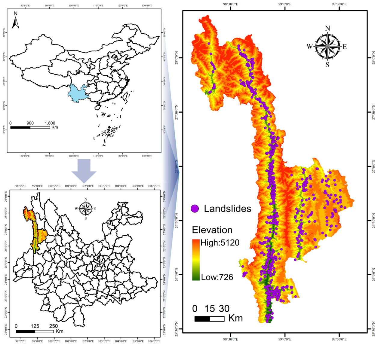
The study area is located in northwestern Yunnan Province, China (
Figure 1). It covers an area of approximately 14,703 km
2, with elevations ranging from about 740 m to 5130 m, yielding a local relief of 4390 m (
Figure 1). The study area spans longitudes 98°39′E to 99°39′E and latitudes 25°33′N to 28°23′N. It administratively includes Lushui City, Fugong County, Gongshan County, and Lanping County. The region is characterized by a series of north–south trending high mountains and deep valleys, with significant topographic relief [
41]. Geologically, the study area consists of alternating weak and hard rock strata, leading to poor rock slope stability [
42]. Despite a high vegetation cover, the soils are thin and infertile, and root systems are poorly developed. Under the combined effects of strong winds and intense rainfall, the area is highly susceptible to geohazards such as landslides, collapses, and debris flows [
7]. Owing to its rugged topography, complex lithological conditions, and abundant precipitation, geoenvironmental safety is a prominent concern in the study area [
43].
Figure 1 shows the geographic location, topographic setting, and landslide inventory distribution of the study area.
2.3. Predictor Variables Generation and CF-Assisted Non-Landslide Sample Construction
For landslide susceptibility modeling in Nujiang Prefecture, a comprehensive set of predictor variables was derived from multi-source geospatial data, including digital elevation model (DEM), remote sensing imagery, geological maps, meteorological records, and land-use datasets. Spatial analysis modules in ArcGIS 10.8 and ENVI 5.3 were adopted for data preprocessing, classification, and spatial interpolation. In addition to generating environmental conditioning factors, the Certainty Factor (CF) model was used in the data-preparation stage to support reliable non-landslide sample construction.
Specifically, CF values were first calculated for each class of the conditioning factors to quantify the empirical association between landslide occurrence and different environmental conditions. These CF values were then overlaid in GIS to generate an initial CF-based landslide susceptibility map. Areas with low initial susceptibility were regarded as relatively reliable non-landslide candidate zones. Known landslide locations were excluded from these candidate zones, and non-landslide samples were randomly selected from the remaining low-susceptibility areas. Accordingly, 561 non-landslide samples were randomly selected to match the 561 mapped landslide samples, resulting in a balanced dataset with a 1:1 landslide/non-landslide sampling ratio. No additional distance buffer was applied around known landslide locations; instead, the CF-based low-susceptibility constraint was used to avoid selecting negative samples from geomorphologically unstable or landslide-prone areas. After sample construction, the final landslide/non-landslide dataset was split into 80% training and 20% testing subsets using stratified random sampling to maintain the label distribution.
It should be noted that the CF values were not used as direct input features, model weights, or prior probabilities in the HSE model. After the landslide/non-landslide sample dataset was constructed, the HSE framework learned directly from the standardized environmental covariates and the probability outputs of the base learners.
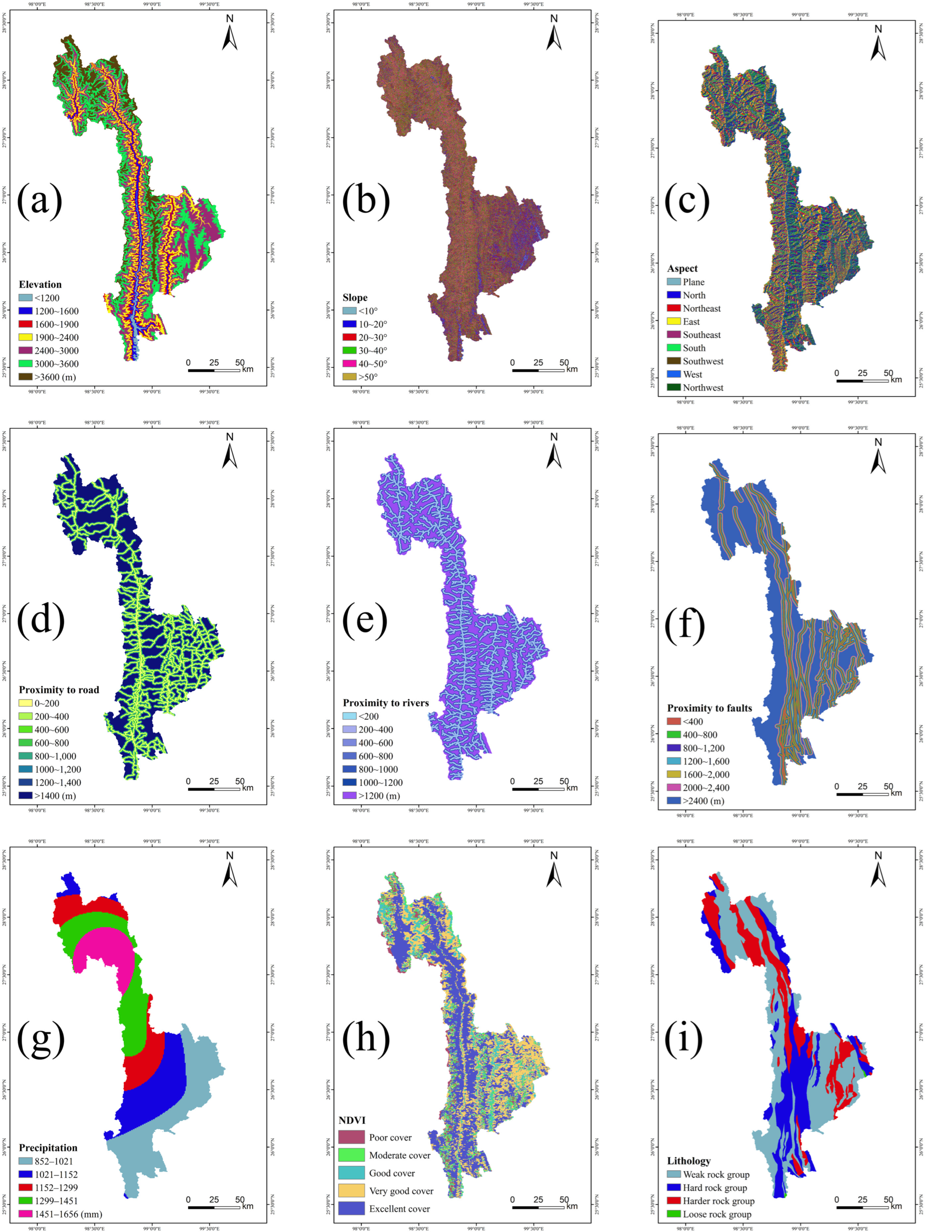
Topographic variables constitute the fundamental conditioning factors for landslide development, extracted directly from DEM via geometric analysis. Elevation was classified in accordance with the vertical climatic zones of Nujiang, with CF analysis revealing that elevations below 1900 m correspond to extremely high landslide susceptibility, driven by intensive human engineering activities and concentrated fluvial systems. Slope angle, a critical index of slope stability, was divided into six gradient classes, and CF results indicated that slopes ranging from 10° to 30° exhibit the highest landslide probability due to favorable mechanical conditions for failure. Aspect was categorized into nine directional classes to reflect differences in solar radiation, vegetation cover, and soil moisture, with its spatial distribution and CF values integrated as a proxy for indirect topoclimatic controls on landslides.
Geological and hydrological variables were constructed to represent the intrinsic geological stability and fluvial erosion effects. Lithology was grouped into four classes (soft rock, hard rock, harder rock, and loose rock) based on stratigraphic properties, where harder rock formations with soft–hard interbeds show the highest landslide susceptibility as soft layers act as natural sliding planes. Proximity to rivers was generated using multi-ring buffers at 200 m intervals, with CF values confirming that areas within 600 m of river channels are strongly influenced by fluvial undercutting and soil softening. Proximity to faults was analyzed using 400 m interval buffers. All distance classes within 2400 m of fault structures exhibit positive CF values, with relatively high values at 400–800 m, 1200–1600 m, and 1600–2000 m, while lower values occur at 800–1200 m and 2000–2400 m. Beyond 2400 m, CF values become negative, indicating reduced landslide susceptibility far from fault zones. This pattern suggests that fault-related structural disturbance may influence slope instability over a relatively broad and non-monotonic distance range, probably through rock mass fragmentation, secondary fractures, and reduced slope integrity in structurally disturbed zones.
Similarly, anthropogenic disturbances from transportation networks were quantified via road proximity, represented by 200 m radius buffers, capturing slope excavation and blasting effects that directly weaken slope stability and trigger landslide events.
Meteorological and vegetation variables were incorporated to account for external triggering and slope protection effects. Annual precipitation was spatially interpolated from 11 meteorological stations via the Kriging method and classified into five grades, as rainfall infiltration and surface erosion serve as the primary triggering mechanism for rainstorm-type landslides in Nujiang. The Normalized Difference Vegetation Index (NDVI) was derived from Landsat 8 OLI imagery using the red and near-infrared bands, consistent with the 30 m analysis grid adopted in this study. NDVI was calculated as , normalized to a 0–1 range, and divided into five classes. Notably, CF analysis revealed an anomalous positive correlation between NDVI and landslide susceptibility in this alpine valley region, attributed to steep terrain, shallow soils, and underdeveloped vegetation root systems that fail to reinforce slopes upon disturbance.
In total, 9 predictor variables covering topographic, geological, hydrological, meteorological, vegetation, and anthropogenic domains were generated for landslide susceptibility modeling, as illustrated in
Figure 2. The spatial density of landslide points across variable classes and computed CF values (
Table 2) jointly validate the rationality of these variables in characterizing the landslide-prone geospatial conditions of Nujiang Prefecture.
After the initial CF-based landslide susceptibility map was generated, non-landslide samples were selected from the low-susceptibility zones. Known landslide locations were excluded from the candidate non-landslide sampling areas. From the remaining low-susceptibility candidate zones, non-landslide samples were randomly selected at the same number as landslide samples, yielding a 1:1 ratio between landslide and non-landslide samples. No additional distance buffer was applied around known landslide locations; instead, the CF-based low-susceptibility constraint was used to avoid selecting negative samples from geomorphologically unstable or landslide-prone areas. The final landslide/non-landslide sample dataset was then split into 80% training and 20% testing subsets using stratified random sampling to preserve the class distribution.
2.4. Methods
2.4.1. Problem Definition and Framework
Let denote the number of spatial grid cells in the study area, where each cell is characterized by environmental covariates (including geographical coordinates, topographic, geological, and hydrological features) and a binary label ( = 1 for landslide occurrence, = 0 for stability). We aim to predict the landslide occurrence probability for each cell, a task hindered by three critical limitations of conventional landslide susceptibility models: inadequate capture of spatial heterogeneity, poor modeling of nonlinear covariate–landslide relationships, and over-reliance on single-model inference, which compromises robustness in complex geomorphic environments.
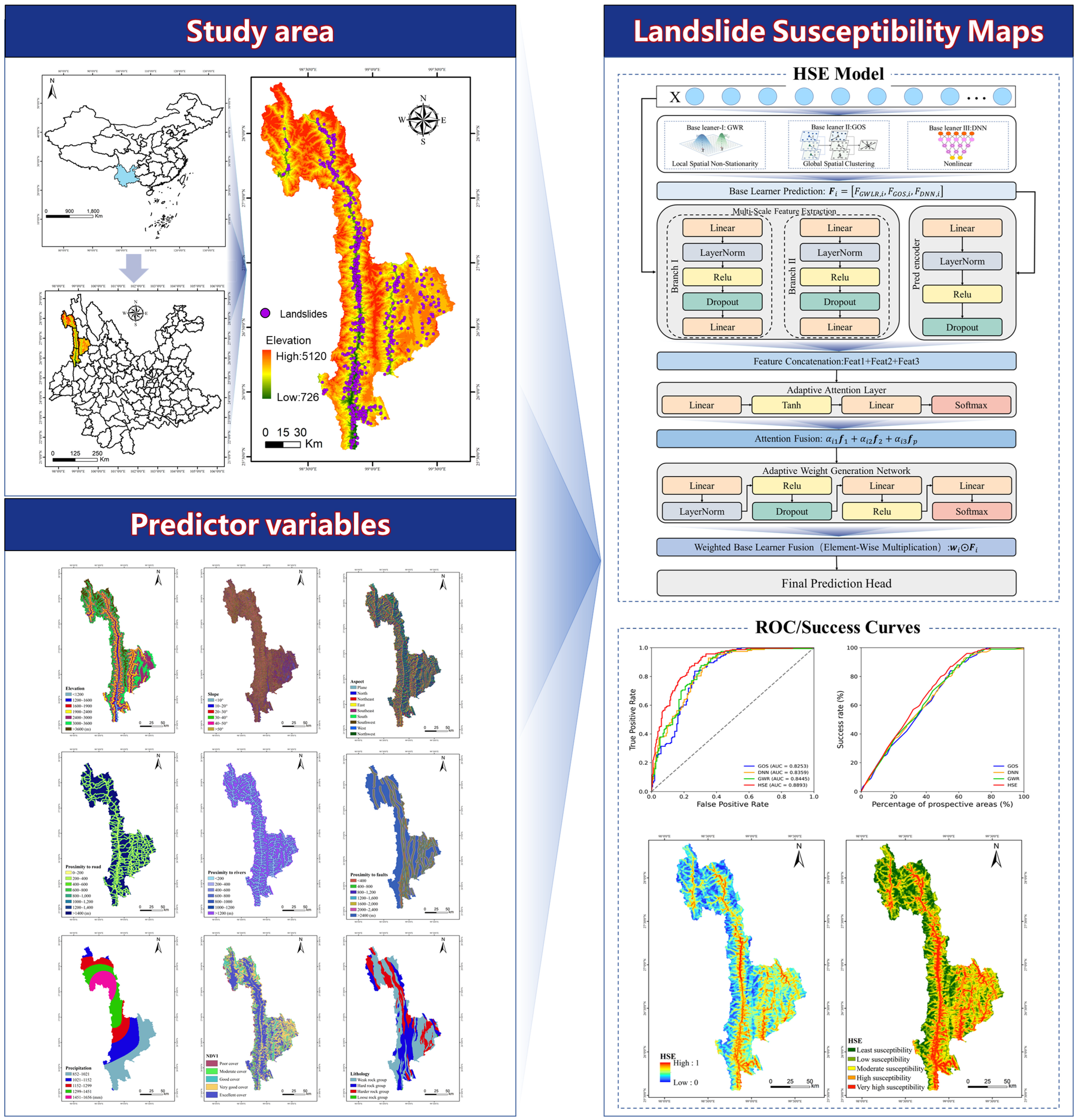
To address these gaps, we develop a two-stage hierarchical spatial adaptive ensemble (HSE) framework (
Figure 3). In the first stage, three complementary base learners are deployed to disentangle diverse landslide-driven patterns: geographically weighted regression (GWR) quantifies spatial non-stationarity, the geographically optimal similarity (GOS) model represents similarity-based local dependence by assuming that locations with similar geo-environmental conditions tend to exhibit similar landslide susceptibility, and a deep neural network (DNN) mines nonlinear covariate interactions. In the second stage, an attention-based deep ensemble model adaptively fuses these base predictions via multi-scale feature extraction and dynamic weight allocation, unifying spatial heterogeneity characterization, nonlinear learning, and ensemble inference into a single cohesive framework. This design delivers more accurate, robust, and geophysically consistent landslide susceptibility assessments.
2.4.2. Design of the Base Learner
Spatial heterogeneity, complex nonlinearity, and geographic similarity represent three core properties of landslide geospatial data. To capture these complementary patterns simultaneously, we adopt three structurally distinct base learners: Geographically Weighted Regression (GWR), Deep neural network (DNN), and Geographically Optimal Similarity (GOS). Their inherent diversity enables the ensemble framework to characterize spatially varying relationships, high-dimensional nonlinear interactions, and local spatial affinity, respectively, thereby improving prediction robustness and generalization.
GWR is introduced to model spatial nonstationarity by constructing location-specific linear regressions with distance-decay spatial weights [
44]. For each spatial location (
), the regression coefficients vary continuously over space rather than being fixed globally:
The coefficients are estimated via weighted least squares:
where
denotes an adaptive bisquare kernel weight matrix. GWR provides explicit spatial interpretability for local landslide-driving mechanisms.
- 2.
Deep neural network
To obtain the reference estimate
, we employ a deep neural network (DNN) with two hidden layers and
ReLU activation functions [
45]. Denote the input vector of the
spatial cell as
. The first hidden layer computes:
where
and
are the weight matrix and bias vector of the first layer. This output is then passed to the second hidden layer:
with
,
defined analogously. Finally, the output layer applies a sigmoid function to produce the landslide occurrence probability:
where
,
are the parameters of the output layer, and
denotes the sigmoid activation function.
This neural network structure enables the model to capture complex nonlinear relationships between environmental covariates and landslide occurrences, automatically learning hierarchical feature interactions to enhance the representation of covariate associations.
- 3.
Geographically Optimal Similarity
GOS performs nonparametric prediction based on the third law of geography: locations with similar geographic environments have similar landslide probabilities [
46]. For each unobserved site t, the multivariate similarity to an observed site k is computed as:
The prediction is obtained by weighted aggregation of highly similar samples:
GOS is a nonparametric similarity-based estimator that predicts landslide susceptibility by weighted aggregation of observed samples with high geo-environmental similarity. Rather than explicitly modeling spatial clustering, GOS relies on a similarity-based model assumption that locations with similar geo-environmental conditions tend to exhibit similar landslide susceptibility. This assumption was used to construct a complementary similarity-based base learner, but it was not independently tested as a stand-alone spatial-dependence hypothesis in the present study area. Therefore, the GOS results should be interpreted as similarity-based predictive evidence rather than as direct validation of an underlying spatial-dependence mechanism. In this way, GOS provides complementary information to GWR and DNN by incorporating environmental similarity into the ensemble framework without imposing a linear functional form.
2.4.3. Multi-Branch Attention-Based Adaptive Ensemble Strategy
Building on the two-stage hierarchical framework proposed in
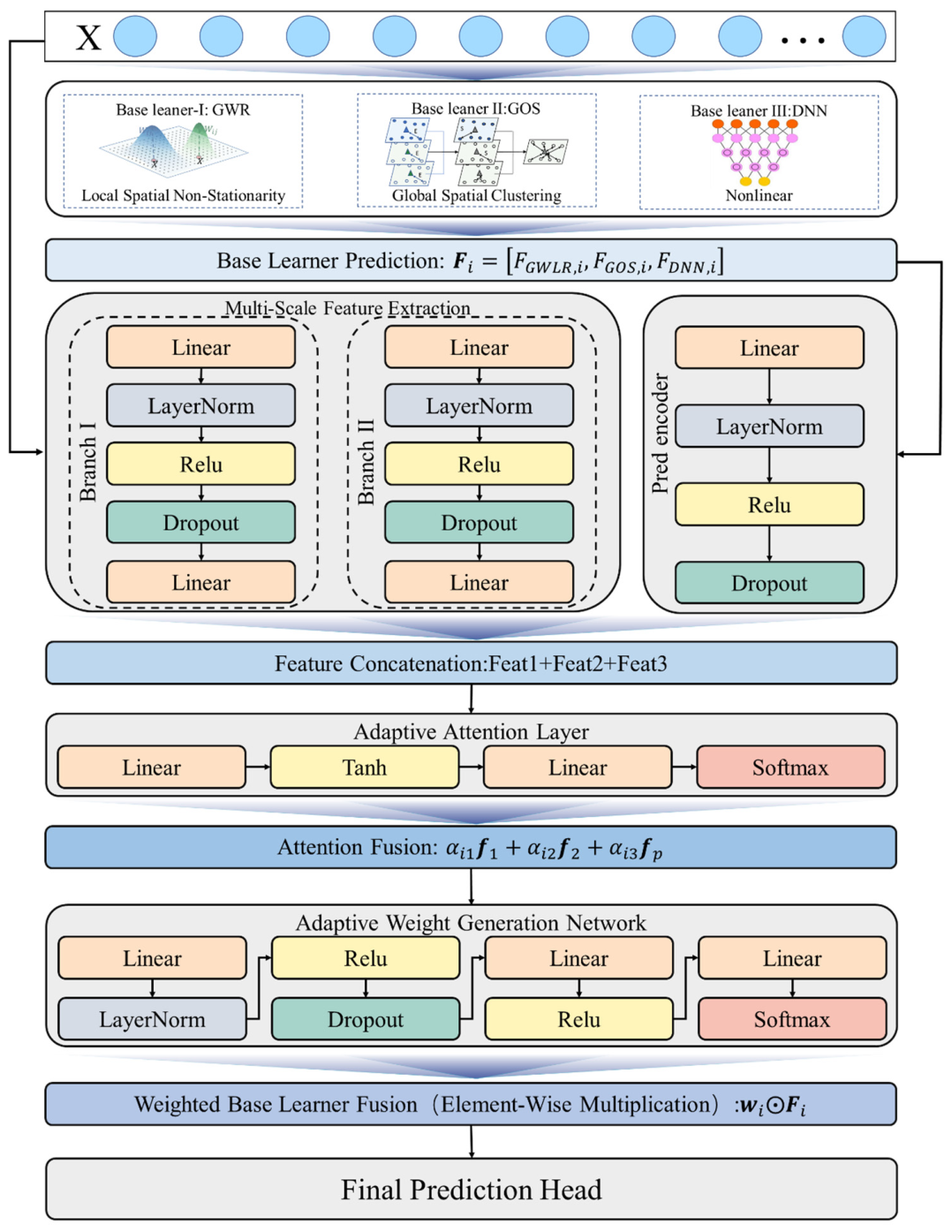
Section 2.4.1, conventional ensemble schemes for landslide susceptibility modeling rely on fixed global weighting or kernel-constrained local fusion, which fail to capture spatial heterogeneity in model reliability. The predictive performance of GWR, GOS and DNN base learners varies sharply across geomorphologically distinct regions, rendering static weight assignments physically inconsistent and prone to reduced robustness. To resolve this limitation, we develop a two-stage probability-level adaptive ensemble architecture that learns location-specific fusion weights by integrating environmental covariates and base-model prediction probabilities (
Figure 4). The proposed HSE network is not designed as an unconstrained end-to-end classifier that refits the entire landslide susceptibility relationship from raw inputs alone. Instead, the GWR, DNN, and GOS base learners are first trained independently and then frozen, and their predicted susceptibility probabilities are used as fixed inputs to the ensemble module. Therefore, the trainable network mainly learns adaptive fusion relationships among base-model outputs and environmental covariates, rather than relearning the full prediction task from scratch.
The network takes two core inputs: the standardized environmental covariate vector for spatial cell i and the base-model prediction vector output by the first-stage learners. We first extract nonlinear feature representations from the environmental covariates through two parallel feature-encoding branches:
here,
and
are two fully connected feature transformation modules that generate complementary high-level representations for topographic, geological and hydrological conditions. These two feature-encoding branches possess distinct expressive capabilities. The wider branch
is dedicated to capturing complex nonlinear interactions among conditioning factors, while the narrower branch
produces more compact features and avoids over-reliance on a single high-dimensional feature projection. Both branches are projected into a latent space of identical dimensionality prior to attention-based fusion, yielding diverse feature representations whose relative contributions are adaptively adjusted via learned attention weights.
To integrate information from base-model predictions, we embed the raw prediction vector into a discriminative latent space via a dedicated encoding module:
where
represents the prediction embedding branch, which distills the complementary strengths of spatial statistical and deep learning-based base learners.
We then concatenate the three latent feature vectors and feed them into an attention network to learn adaptive feature importance weights:
here,
denotes vector concatenation,
is the attention transformation module, and
represents the spatial-channel attention weight vector that emphasizes geophysically meaningful features while suppressing redundant signals.
The attention weights are used to fuse the multi-scale environmental and prediction features into a compact contextual representation:
This fused feature encapsulates local geographic context and cross-model predictive information, forming the basis for location-adaptive weight assignment.
Next, we input the fused contextual feature into a weight generation network to produce sample-specific weights for the three base learners, normalized to ensure probabilistic interpretability:
where
denotes the adaptive weight generation module, and
is the normalized weight vector, with each element quantifying the local contribution of the corresponding base model at cell
.
Finally, the attention-fused features and weight-adjusted base-model predictions are combined to estimate the final landslide occurrence probability:
where
denotes element-wise multiplication,
is the final prediction transformation module, and
is the sigmoid function that constrains
for physically consistent susceptibility quantification.
After the GWR, GOS, and DNN base learners were independently trained and frozen, the attention-based ensemble network was optimized using binary cross-entropy loss. During this stage, only the parameters of the feature-encoding branches, attention module, weight-generation module, and final prediction module were updated, whereas gradients were not propagated back to the base learners. This design abandons fixed global weighting and rigid kernel-constrained fusion while avoiding joint fine-tuning of the base learners.