Article

Attention-Driven Hierarchical Spatial Adaptive Ensemble for Landslide Susceptibility Mapping

1
School of Geosciences and Info-Physics, Central South University, Changsha 410083, China
2
School of Earth Sciences, Yunnan University, Kunming 650500, China
*
Author to whom correspondence should be addressed.
Remote Sens. 2026, 18(12), 1999; https://doi.org/10.3390/rs18121999
Submission received: 7 May 2026 / Revised: 3 June 2026 / Accepted: 11 June 2026 / Published: 16 June 2026

Highlights

What are the main findings?
  • Attention-driven adaptive fusion of GWR, GOS, and DNN learns spatially varying base-learner weights, directly overcoming the fixed-weight and kernel-constrained limitations of conventional ensembles.
  • The attention-based ensemble dynamically allocates location-specific fusion weights conditioned on multi-scale environmental features, enabling the ensemble process to adapt to spatially varying model reliability without any predefined spatial kernel or global stationarity assumption.
What are the implications of the main findings?
  • Explicitly learning spatial heterogeneity during ensemble fusion is essential for reliable landslide susceptibility mapping, and the framework is readily transferable to other geospatial prediction tasks plagued by non-stationarity.
  • The HSE framework produces geomorphologically refined susceptibility maps that avoid over-diffusion of high-risk zones and misclassification of stable terrain, directly supporting targeted field investigation, engineering mitigation prioritization, and land-use zoning.

Abstract

Landslides cause thousands of fatalities and billions in economic losses annually, yet reliable susceptibility mapping across heterogeneous landscapes remains challenging because conventional models assume stationary relationships between landslide occurrence and environmental controls. Ensemble methods, though promising, rely on either globally fixed aggregation weights or kernel-constrained local averaging, failing to adapt when the reliability of base models varies nonlinearly across space. To overcome this, we propose a two-stage hierarchical spatial adaptive ensemble (HSE) framework. In stage one, three complementary base learners are deployed: geographically weighted regression (GWR) for local spatial non-stationarity; a geographically optimal similarity (GOS) model, grounded in the Third Law of Geography, to represent similarity-based local dependence; and a deep neural network (DNN) for nonlinear covariate interactions. In stage two, a multi-branch attention-based network learns spatially varying fusion weights via multi-scale feature extraction, abandoning fixed weights or kernel constraints. We validate HSE on a typical landslide-prone catchment, comparing against single models (GWR, DNN, GOS). Results demonstrate that our method consistently achieves superior predictive accuracy, spatial consistency, and out-of-sample robustness. Moreover, the attention-derived spatially varying weights provide interpretable insights into where each base learner dominates, bridging predictive performance with geophysical interpretability. These findings confirm that explicitly learning spatial heterogeneity during ensemble fusion is essential for reliable landslide susceptibility mapping, with strong potential for transfer to other geospatial prediction tasks.

1. Introduction

Landslides are among the most destructive geological hazards, causing severe casualties and economic losses in mountainous regions [1,2,3,4,5,6]. With climate change intensifying extreme rainfall and human activities expanding into vulnerable terrain, landslide frequency and impact are projected to rise [7,8,9,10,11,12,13,14,15]. Accurate landslide susceptibility mapping (LSM) is thus critical for disaster risk reduction and land-use planning [16,17,18,19,20].
Landslide susceptibility assessment has long relied on data-driven modeling approaches, which have evolved progressively to address the complex controls of landslide occurrence [17,21,22,23,24,25]. Early efforts were dominated by spatial statistical and regression-based models (e.g., geographically weighted regression, logistic regression), which explicitly account for spatial autocorrelation and non-stationarity but are constrained by linearity assumptions and limited ability to capture complex, multi-factor interactions [26]. These were later complemented by classical machine learning methods (e.g., random forests, support vector machines), which improved predictive performance by learning nonlinear relationships from environmental covariates, yet still operate as global models that fail to adapt to spatially varying landslide-controlling mechanisms [27,28].
With advances in deep learning, deep neural network (DNN) architectures have been introduced to model high-dimensional environmental features, demonstrating strong discriminative power for landslide susceptibility mapping [29,30,31]. However, these data-hungry models often overlook inherent spatial topological dependencies in geomorphic systems, and tend to overfit in data-sparse mountainous regions, limiting their generalization across heterogeneous landscapes [32]. To mitigate the uncertainty of single-model inference, conventional ensemble strategies (e.g., simple averaging, stacking) have been adopted to combine outputs from multiple learners, but these rely on fixed, globally defined weights that do not adjust to spatially varying model reliability, leading to suboptimal performance in complex alpine canyon environments [33].
Despite these advances, three fundamental limitations persist. First, global models (statistical or deep) assume stationary relationships between covariates and landslide occurrence, thus failing to capture spatial heterogeneity [32,34]. Second, while deep learning can represent nonlinear interactions, it typically ignores spatial structure and overfits in data-scarce regions; linear or shallow models, conversely, cannot adequately characterize coupled topographic–hydrological–geological nonlinearities [35,36,37]. Third, no single model performs optimally across all geomorphic domains, and conventional ensembles (averaging, stacking) rely on globally fixed aggregation weights, unable to adapt to spatially varying model reliability [38,39,40].
To overcome these challenges, we propose a two-stage hierarchical spatial adaptive ensemble learning (HSE) framework. In the first stage, three complementary base learners are deployed: geographically weighted regression (GWR) for spatial non-stationarity; a geographically optimal similarity (GOS) model for similarity-based local dependence based on the Third Law of Geography; and a deep neural network (DNN) for nonlinear covariate interactions. In the second stage, a multi-branch attention-based deep ensemble network learns location-specific fusion weights via multi-scale feature extraction and dynamic weight allocation, abandoning fixed global or kernel-constrained strategies. A two-stage training strategy was adopted. The GWR, GOS, and DNN base learners were first trained independently, and their predicted probabilities were then treated as fixed inputs to the attention-based ensemble network. Only the second-stage ensemble network was optimized using binary cross-entropy loss to learn adaptive fusion weights.
This work introduces two advances over conventional ensemble methods. First, the framework explicitly accounts for the three fundamental properties of landslide geospatial distribution—non-stationarity, local similarity, and nonlinearity—through a heterogeneous set of base learners that includes a geographically optimal similarity model based on the Third Law of Geography. Second, instead of relying on fixed global weights or kernel-constrained local averaging, we develop an attention-based deep ensemble network that learns spatially varying fusion weights directly from environmental covariates and base predictions, thereby adapting the ensemble process to the nonlinear constraints imposed by spatial heterogeneity.
We validate the framework on a typical landslide-prone area. Comparisons with single-model baselines and static ensemble strategies, together with ablation studies, demonstrate superior predictive accuracy, spatial consistency, and robustness. These results confirm that explicitly characterizing and adaptively learning spatial heterogeneity during model ensemble is critical for reliable landslide susceptibility mapping.

2. Materials and Methods

2.1. Study Area

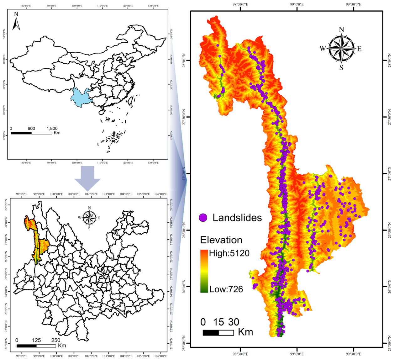
The study area is located in northwestern Yunnan Province, China (Figure 1). It covers an area of approximately 14,703 km2, with elevations ranging from about 740 m to 5130 m, yielding a local relief of 4390 m (Figure 1). The study area spans longitudes 98°39′E to 99°39′E and latitudes 25°33′N to 28°23′N. It administratively includes Lushui City, Fugong County, Gongshan County, and Lanping County. The region is characterized by a series of north–south trending high mountains and deep valleys, with significant topographic relief [41]. Geologically, the study area consists of alternating weak and hard rock strata, leading to poor rock slope stability [42]. Despite a high vegetation cover, the soils are thin and infertile, and root systems are poorly developed. Under the combined effects of strong winds and intense rainfall, the area is highly susceptible to geohazards such as landslides, collapses, and debris flows [7]. Owing to its rugged topography, complex lithological conditions, and abundant precipitation, geoenvironmental safety is a prominent concern in the study area [43]. Figure 1 shows the geographic location, topographic setting, and landslide inventory distribution of the study area.

2.2. Data Sources

The topographic predictors employed in this study—including elevation, slope gradient, slope aspect—were derived from the 30 m resolution Shuttle Radar Topography Mission (SRTM) Version 3 Digital Elevation Model (DEM) dataset, referenced to the GCS_WGS_1984 coordinate system. To guarantee spatial consistency for integrated analysis, all input datasets were uniformly projected to GCS_WGS_1984 and resampled to a consistent 30 m × 30 m spatial resolution.
Remote sensing imagery and basic geographic/thematic datasets were sourced from authoritative public platforms, local government agencies, and published regional monographs, with detailed source information summarized in Table 1. Landsat 8 OLI imagery was obtained from the Geospatial Data Cloud for NDVI derivation, while high-resolution Google Earth imagery was acquired from the BIGEMAP mapping platform for auxiliary visual interpretation and validation. Additional thematic datasets, including historical landslide inventories, meteorological observations, road networks, and geological features, were collected from official regional authorities and national geospatial databases. The historical landslide inventory used in this study contains 561 mapped landslide points, which were used as positive samples for model training and evaluation.

2.3. Predictor Variables Generation and CF-Assisted Non-Landslide Sample Construction

For landslide susceptibility modeling in Nujiang Prefecture, a comprehensive set of predictor variables was derived from multi-source geospatial data, including digital elevation model (DEM), remote sensing imagery, geological maps, meteorological records, and land-use datasets. Spatial analysis modules in ArcGIS 10.8 and ENVI 5.3 were adopted for data preprocessing, classification, and spatial interpolation. In addition to generating environmental conditioning factors, the Certainty Factor (CF) model was used in the data-preparation stage to support reliable non-landslide sample construction.
Specifically, CF values were first calculated for each class of the conditioning factors to quantify the empirical association between landslide occurrence and different environmental conditions. These CF values were then overlaid in GIS to generate an initial CF-based landslide susceptibility map. Areas with low initial susceptibility were regarded as relatively reliable non-landslide candidate zones. Known landslide locations were excluded from these candidate zones, and non-landslide samples were randomly selected from the remaining low-susceptibility areas. Accordingly, 561 non-landslide samples were randomly selected to match the 561 mapped landslide samples, resulting in a balanced dataset with a 1:1 landslide/non-landslide sampling ratio. No additional distance buffer was applied around known landslide locations; instead, the CF-based low-susceptibility constraint was used to avoid selecting negative samples from geomorphologically unstable or landslide-prone areas. After sample construction, the final landslide/non-landslide dataset was split into 80% training and 20% testing subsets using stratified random sampling to maintain the label distribution.
It should be noted that the CF values were not used as direct input features, model weights, or prior probabilities in the HSE model. After the landslide/non-landslide sample dataset was constructed, the HSE framework learned directly from the standardized environmental covariates and the probability outputs of the base learners.
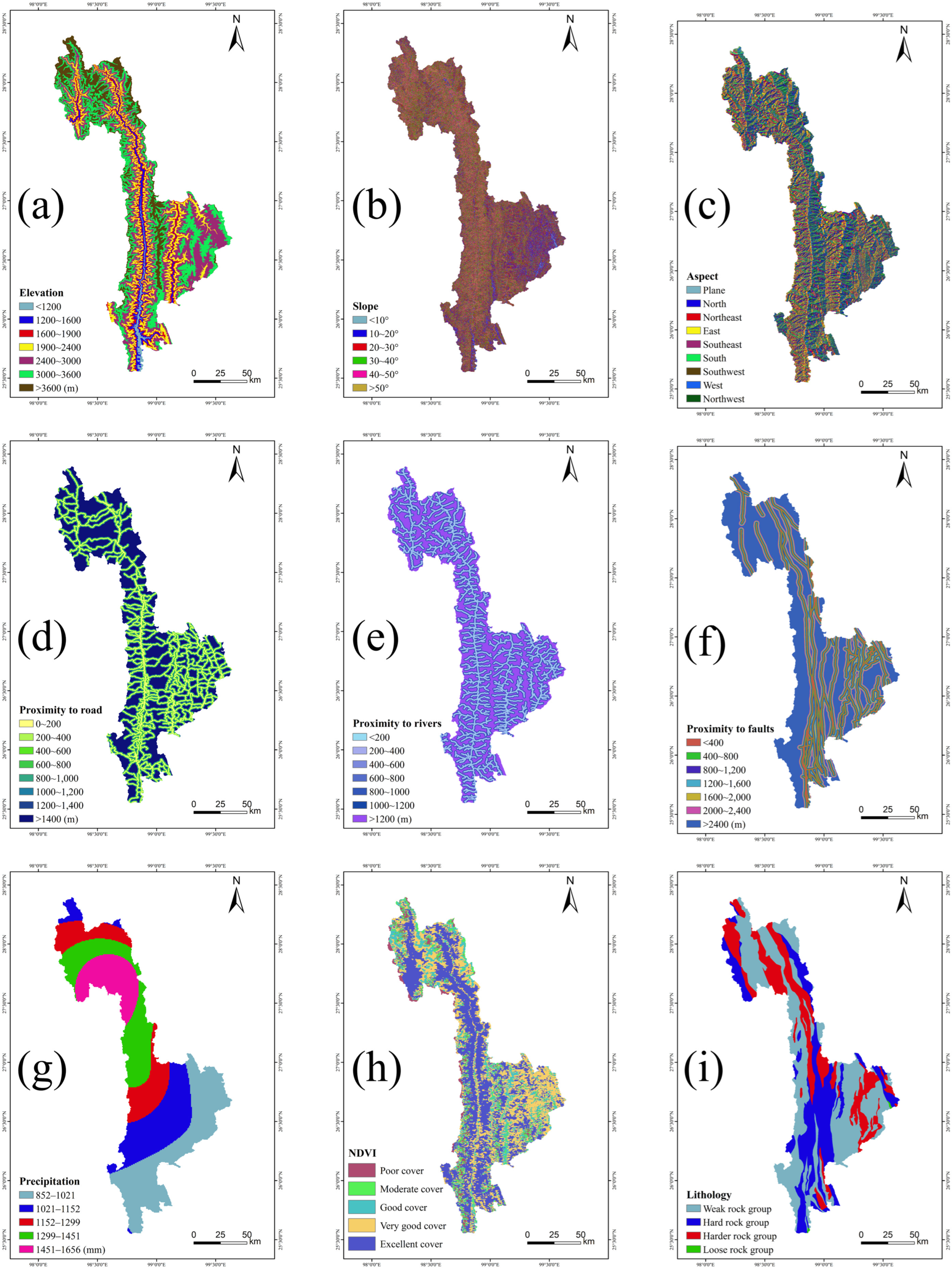
Topographic variables constitute the fundamental conditioning factors for landslide development, extracted directly from DEM via geometric analysis. Elevation was classified in accordance with the vertical climatic zones of Nujiang, with CF analysis revealing that elevations below 1900 m correspond to extremely high landslide susceptibility, driven by intensive human engineering activities and concentrated fluvial systems. Slope angle, a critical index of slope stability, was divided into six gradient classes, and CF results indicated that slopes ranging from 10° to 30° exhibit the highest landslide probability due to favorable mechanical conditions for failure. Aspect was categorized into nine directional classes to reflect differences in solar radiation, vegetation cover, and soil moisture, with its spatial distribution and CF values integrated as a proxy for indirect topoclimatic controls on landslides.
Geological and hydrological variables were constructed to represent the intrinsic geological stability and fluvial erosion effects. Lithology was grouped into four classes (soft rock, hard rock, harder rock, and loose rock) based on stratigraphic properties, where harder rock formations with soft–hard interbeds show the highest landslide susceptibility as soft layers act as natural sliding planes. Proximity to rivers was generated using multi-ring buffers at 200 m intervals, with CF values confirming that areas within 600 m of river channels are strongly influenced by fluvial undercutting and soil softening. Proximity to faults was analyzed using 400 m interval buffers. All distance classes within 2400 m of fault structures exhibit positive CF values, with relatively high values at 400–800 m, 1200–1600 m, and 1600–2000 m, while lower values occur at 800–1200 m and 2000–2400 m. Beyond 2400 m, CF values become negative, indicating reduced landslide susceptibility far from fault zones. This pattern suggests that fault-related structural disturbance may influence slope instability over a relatively broad and non-monotonic distance range, probably through rock mass fragmentation, secondary fractures, and reduced slope integrity in structurally disturbed zones.
Similarly, anthropogenic disturbances from transportation networks were quantified via road proximity, represented by 200 m radius buffers, capturing slope excavation and blasting effects that directly weaken slope stability and trigger landslide events.
Meteorological and vegetation variables were incorporated to account for external triggering and slope protection effects. Annual precipitation was spatially interpolated from 11 meteorological stations via the Kriging method and classified into five grades, as rainfall infiltration and surface erosion serve as the primary triggering mechanism for rainstorm-type landslides in Nujiang. The Normalized Difference Vegetation Index (NDVI) was derived from Landsat 8 OLI imagery using the red and near-infrared bands, consistent with the 30 m analysis grid adopted in this study. NDVI was calculated as N I R R e d / N I R + R e d , normalized to a 0–1 range, and divided into five classes. Notably, CF analysis revealed an anomalous positive correlation between NDVI and landslide susceptibility in this alpine valley region, attributed to steep terrain, shallow soils, and underdeveloped vegetation root systems that fail to reinforce slopes upon disturbance.
In total, 9 predictor variables covering topographic, geological, hydrological, meteorological, vegetation, and anthropogenic domains were generated for landslide susceptibility modeling, as illustrated in Figure 2. The spatial density of landslide points across variable classes and computed CF values (Table 2) jointly validate the rationality of these variables in characterizing the landslide-prone geospatial conditions of Nujiang Prefecture.
After the initial CF-based landslide susceptibility map was generated, non-landslide samples were selected from the low-susceptibility zones. Known landslide locations were excluded from the candidate non-landslide sampling areas. From the remaining low-susceptibility candidate zones, non-landslide samples were randomly selected at the same number as landslide samples, yielding a 1:1 ratio between landslide and non-landslide samples. No additional distance buffer was applied around known landslide locations; instead, the CF-based low-susceptibility constraint was used to avoid selecting negative samples from geomorphologically unstable or landslide-prone areas. The final landslide/non-landslide sample dataset was then split into 80% training and 20% testing subsets using stratified random sampling to preserve the class distribution.

2.4. Methods

2.4.1. Problem Definition and Framework

Let N denote the number of spatial grid cells in the study area, where each cell v i is characterized by m environmental covariates x i = x i 1 , , x i m (including geographical coordinates, topographic, geological, and hydrological features) and a binary label y i ( y i = 1 for landslide occurrence, y i = 0 for stability). We aim to predict the landslide occurrence probability P y i x i for each cell, a task hindered by three critical limitations of conventional landslide susceptibility models: inadequate capture of spatial heterogeneity, poor modeling of nonlinear covariate–landslide relationships, and over-reliance on single-model inference, which compromises robustness in complex geomorphic environments.
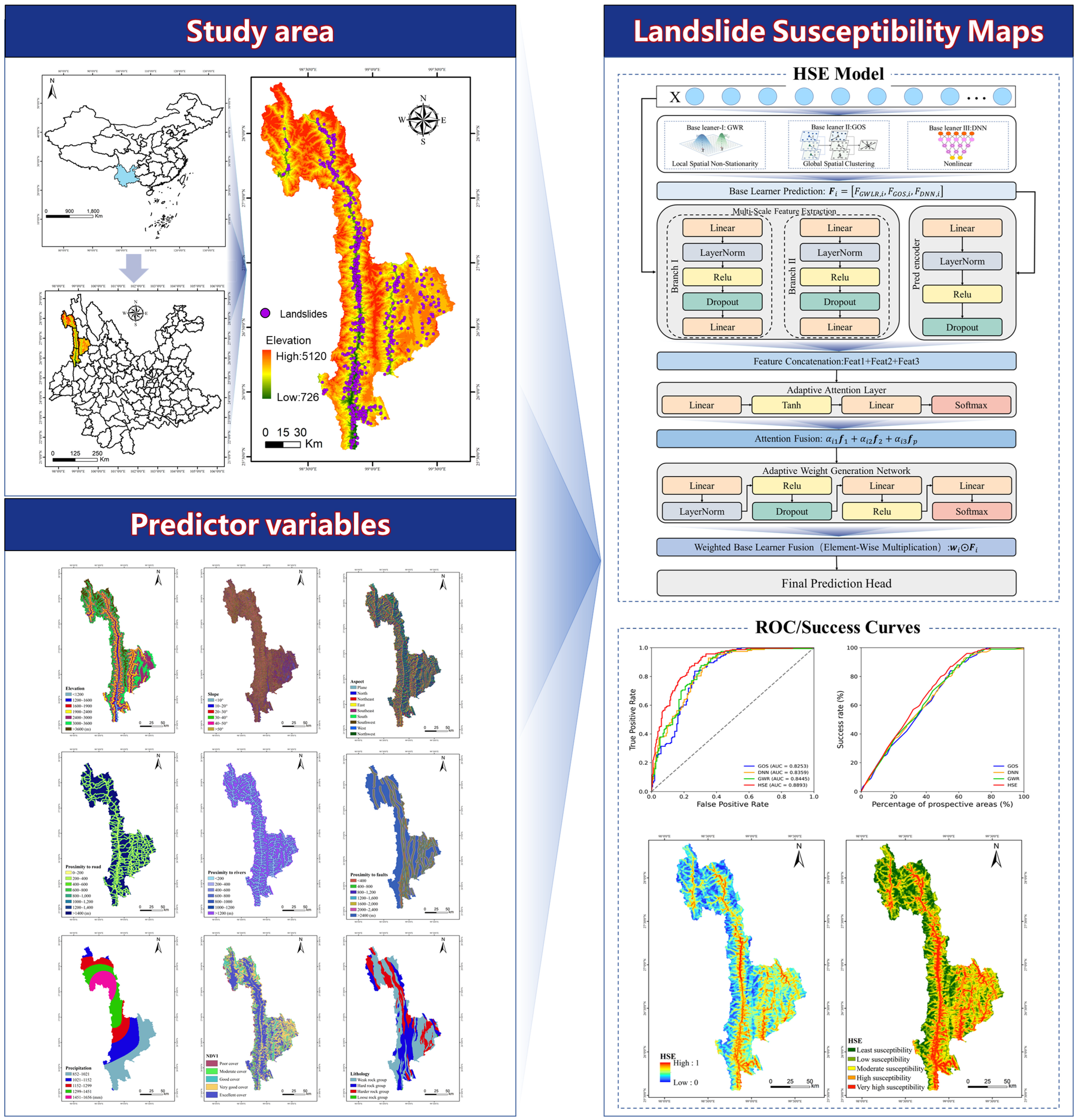
To address these gaps, we develop a two-stage hierarchical spatial adaptive ensemble (HSE) framework (Figure 3). In the first stage, three complementary base learners are deployed to disentangle diverse landslide-driven patterns: geographically weighted regression (GWR) quantifies spatial non-stationarity, the geographically optimal similarity (GOS) model represents similarity-based local dependence by assuming that locations with similar geo-environmental conditions tend to exhibit similar landslide susceptibility, and a deep neural network (DNN) mines nonlinear covariate interactions. In the second stage, an attention-based deep ensemble model adaptively fuses these base predictions via multi-scale feature extraction and dynamic weight allocation, unifying spatial heterogeneity characterization, nonlinear learning, and ensemble inference into a single cohesive framework. This design delivers more accurate, robust, and geophysically consistent landslide susceptibility assessments.

2.4.2. Design of the Base Learner

Spatial heterogeneity, complex nonlinearity, and geographic similarity represent three core properties of landslide geospatial data. To capture these complementary patterns simultaneously, we adopt three structurally distinct base learners: Geographically Weighted Regression (GWR), Deep neural network (DNN), and Geographically Optimal Similarity (GOS). Their inherent diversity enables the ensemble framework to characterize spatially varying relationships, high-dimensional nonlinear interactions, and local spatial affinity, respectively, thereby improving prediction robustness and generalization.
  • Geographically Weighted Regression
GWR is introduced to model spatial nonstationarity by constructing location-specific linear regressions with distance-decay spatial weights [44]. For each spatial location ( u i , v i ), the regression coefficients vary continuously over space rather than being fixed globally:
y i = β 0 u i , v i + j = 1 p β j u i , v i x i j + ε i
The coefficients are estimated via weighted least squares:
β ^ u i , v i = X T W u i , v i X 1 X T W u i , v i Y
where W u i , v i denotes an adaptive bisquare kernel weight matrix. GWR provides explicit spatial interpretability for local landslide-driving mechanisms.
2.
Deep neural network
To obtain the reference estimate p i = P y i = 1 x i , we employ a deep neural network (DNN) with two hidden layers and ReLU activation functions [45]. Denote the input vector of the i t h spatial cell as h 0 = x i . The first hidden layer computes:
h 1 = R e L U ( W 1 h 0 + b 1 )
where W 1 and b 1 are the weight matrix and bias vector of the first layer. This output is then passed to the second hidden layer:
h 2 = R e L U ( W 2 h 1 + b 2 )
with W 2 , b 2   defined analogously. Finally, the output layer applies a sigmoid function to produce the landslide occurrence probability:
p i = σ ( W 3 h 2 + b 3 )
where W 3 , b 3 are the parameters of the output layer, and σ ( ) denotes the sigmoid activation function.
This neural network structure enables the model to capture complex nonlinear relationships between environmental covariates and landslide occurrences, automatically learning hierarchical feature interactions to enhance the representation of covariate associations.
3.
Geographically Optimal Similarity
GOS performs nonparametric prediction based on the third law of geography: locations with similar geographic environments have similar landslide probabilities [46]. For each unobserved site t, the multivariate similarity to an observed site k is computed as:
E i k , t = e x p X k i X t i 2 σ i 2 , S k , t = m i n i E i ( k , t )
The prediction is obtained by weighted aggregation of highly similar samples:
y ^ t = k = K S k , t y k k = K S k , t
GOS is a nonparametric similarity-based estimator that predicts landslide susceptibility by weighted aggregation of observed samples with high geo-environmental similarity. Rather than explicitly modeling spatial clustering, GOS relies on a similarity-based model assumption that locations with similar geo-environmental conditions tend to exhibit similar landslide susceptibility. This assumption was used to construct a complementary similarity-based base learner, but it was not independently tested as a stand-alone spatial-dependence hypothesis in the present study area. Therefore, the GOS results should be interpreted as similarity-based predictive evidence rather than as direct validation of an underlying spatial-dependence mechanism. In this way, GOS provides complementary information to GWR and DNN by incorporating environmental similarity into the ensemble framework without imposing a linear functional form.

2.4.3. Multi-Branch Attention-Based Adaptive Ensemble Strategy

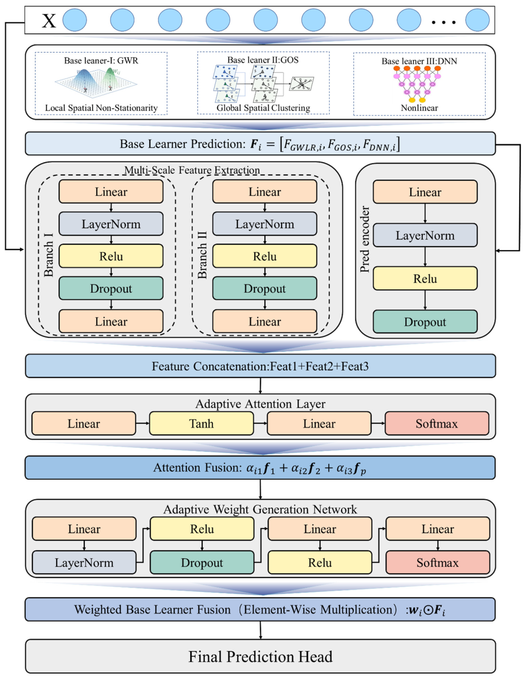
Building on the two-stage hierarchical framework proposed in Section 2.4.1, conventional ensemble schemes for landslide susceptibility modeling rely on fixed global weighting or kernel-constrained local fusion, which fail to capture spatial heterogeneity in model reliability. The predictive performance of GWR, GOS and DNN base learners varies sharply across geomorphologically distinct regions, rendering static weight assignments physically inconsistent and prone to reduced robustness. To resolve this limitation, we develop a two-stage probability-level adaptive ensemble architecture that learns location-specific fusion weights by integrating environmental covariates and base-model prediction probabilities (Figure 4). The proposed HSE network is not designed as an unconstrained end-to-end classifier that refits the entire landslide susceptibility relationship from raw inputs alone. Instead, the GWR, DNN, and GOS base learners are first trained independently and then frozen, and their predicted susceptibility probabilities are used as fixed inputs to the ensemble module. Therefore, the trainable network mainly learns adaptive fusion relationships among base-model outputs and environmental covariates, rather than relearning the full prediction task from scratch.
The network takes two core inputs: the standardized environmental covariate vector for spatial cell i and the base-model prediction vector output by the first-stage learners. We first extract nonlinear feature representations from the environmental covariates through two parallel feature-encoding branches:
f 1 = F 1 X i ,   f 2 = F 2 X i
here, F 1 and F 2 are two fully connected feature transformation modules that generate complementary high-level representations for topographic, geological and hydrological conditions. These two feature-encoding branches possess distinct expressive capabilities. The wider branch F 1 is dedicated to capturing complex nonlinear interactions among conditioning factors, while the narrower branch F 2 produces more compact features and avoids over-reliance on a single high-dimensional feature projection. Both branches are projected into a latent space of identical dimensionality prior to attention-based fusion, yielding diverse feature representations whose relative contributions are adaptively adjusted via learned attention weights.
To integrate information from base-model predictions, we embed the raw prediction vector into a discriminative latent space via a dedicated encoding module:
f p = E F i
where E represents the prediction embedding branch, which distills the complementary strengths of spatial statistical and deep learning-based base learners.
We then concatenate the three latent feature vectors and feed them into an attention network to learn adaptive feature importance weights:
α i = s o f t m a x A f 1 f 2 f p
here, denotes vector concatenation, A is the attention transformation module, and α i   represents the spatial-channel attention weight vector that emphasizes geophysically meaningful features while suppressing redundant signals.
The attention weights are used to fuse the multi-scale environmental and prediction features into a compact contextual representation:
h i = α i 1 f 1 + α i 2 f 2 + α i 3 f p
This fused feature h i encapsulates local geographic context and cross-model predictive information, forming the basis for location-adaptive weight assignment.
Next, we input the fused contextual feature into a weight generation network to produce sample-specific weights for the three base learners, normalized to ensure probabilistic interpretability:
w i = s o f t m a x W h i f p
where W denotes the adaptive weight generation module, and w i = w G W L R , i , w G O S , i , w D N N , i is the normalized weight vector, with each element quantifying the local contribution of the corresponding base model at cell   i .
Finally, the attention-fused features and weight-adjusted base-model predictions are combined to estimate the final landslide occurrence probability:
p i = σ P h i w i F i
where denotes element-wise multiplication, P is the final prediction transformation module, and σ ( ) is the sigmoid function that constrains p i 0 ,   1 for physically consistent susceptibility quantification.
After the GWR, GOS, and DNN base learners were independently trained and frozen, the attention-based ensemble network was optimized using binary cross-entropy loss. During this stage, only the parameters of the feature-encoding branches, attention module, weight-generation module, and final prediction module were updated, whereas gradients were not propagated back to the base learners. This design abandons fixed global weighting and rigid kernel-constrained fusion while avoiding joint fine-tuning of the base learners.


3. Results

3.1. Landslide Susceptibility Modelling

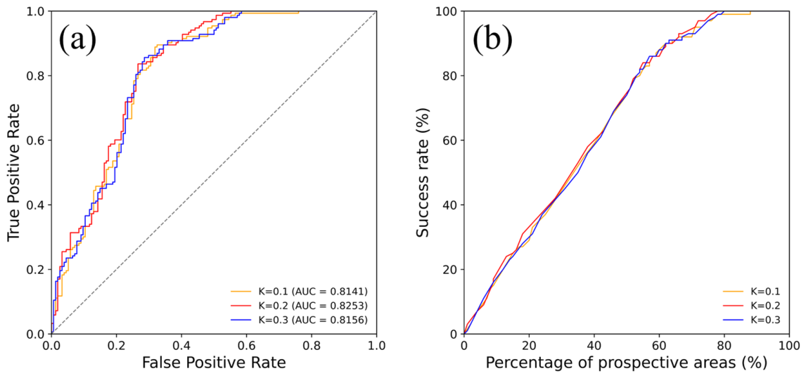
In this study, a HSE framework was established for landslide susceptibility modeling. The input dataset included spatial coordinates and multiple environmental conditioning factors, with each sample labeled as landslide or non-landslide. The non-landslide samples were randomly selected from the CF-derived low-susceptibility candidate zones described in Section 2.3, using a landslide/non-landslide sampling ratio of 1:1. All features were standardized using StandardScaler to eliminate scaling effects, and the dataset was split into 80% training and 20% test sets via stratified random sampling to maintain label distribution. Three base models were trained to generate initial susceptibility probabilities: a geographically weighted regression (GWR) model with an adaptive bisquare kernel, for which the adaptive bandwidth was selected by minimizing the Corrected Akaike Information Criterion (AICc) within the training set. The selected adaptive bandwidth was 306 nearest training samples, which was then used for final GWR prediction; a deep neural network (DNN) classifier with hidden layers (256, 64), maximum 300 iterations, and sigmoid calibration via 5-fold cross-validation; and a Geographically Optimal Similarity (GOS) model with the optimal-similarity selection parameter κ set to 0.2. In GOS, κ is a quantile-based parameter that controls the proportion of highly similar training samples retained for prediction, rather than a geographic bandwidth. Thus, κ = 0.2 means that the top 20% most environmentally similar samples were used for similarity-weighted prediction. To justify this setting, we further tested κ = 0.1 , 0.2, and 0.3. As shown in Figure 5, the ROC and success-rate curves remain highly consistent, indicating that the GOS model is not sensitive to moderate variations in κ . Therefore, κ = 0.2 was retained because it provides a reasonable balance between local similarity representation and prediction stability.
The GWR, GOS, and DNN base learners were first trained independently using the training split and then frozen before ensemble learning. Their predicted landslide probabilities were treated as fixed probability-level inputs to the attention-based ensemble network. During ensemble training, only the parameters of the feature-encoding branches, prediction encoder, attention module, weight-generation module, and final prediction head were updated, whereas the parameters of the base learners were not fine-tuned. Therefore, gradients from the ensemble loss were not propagated back to the DNN base learner, avoiding gradient conflicts and preventing fine-tuning-induced data leakage. In this study, the ensemble training stage refers only to the internal optimization of the attention-based ensemble network after the base learners have been frozen. The model consists of two parallel feature extraction branches: the first branch contains a fully connected layer mapping the input feature dimension to 512 neurons, followed by layer normalization, ReLU activation, dropout with a rate of 0.15, and a projection to 128 dimensions; the second branch maps input features to 256 neurons, applies layer normalization, ReLU activation, and dropout, then also compresses features to 128 dimensions. A separate prediction encoder processes the three base-model probability outputs through a 128-dimensional fully connected layer with layer normalization, ReLU activation, and dropout. An attention mechanism fuses the three groups of features using a two-layer network (128 × 3 to 128, then to 3) with Tanh activation and Softmax normalization to produce adaptive fusion weights. The weight-generation network takes fused features as input, passes through 256-to-128 and 128-to-64 fully connected layers with layer normalization and dropout, and finally outputs three dynamic weights for the base learners via Softmax. The final predictor concatenates fused features and weighted base predictions, then maps them through 256 and 128 hidden layers to a single output, with sigmoid activation to produce landslide susceptibility probabilities. All linear layers were initialized using the Xavier uniform distribution, and layer normalization layers were initialized with unit weight and zero bias. The model was optimized using the AdamW optimizer with a learning rate of 5 × 10⁻³ and weight decay of 1 × 10⁻⁵. Binary cross-entropy (BCELoss) was employed as the loss function to measure the discrepancy between predicted probabilities and true labels. The model was trained for 250 epochs, and the final checkpoint was selected within the training procedure, while the held-out test set was used only for final performance evaluation. Through adaptive attention-based feature fusion and dynamic weighting of base model predictions, the proposed framework effectively integrates geospatial interpretability and deep learning expressiveness, yielding robust, spatially consistent, and geologically plausible landslide susceptibility predictions.
To reduce the risk of overfitting, several regularization mechanisms were adopted jointly, including Layer Normalization, repeated dropout operations, AdamW weight decay, and the two-stage training strategy with frozen base learners. The dropout rate of 0.15 was used as a moderate regularization setting within this combined strategy, rather than as the only means of controlling overfitting. Since the ensemble module operates on fixed base-model probabilities and standardized environmental covariates, an excessively large dropout rate may suppress useful weak signals required for probability-level fusion. Therefore, the selected dropout setting was used to balance regularization and information preservation.
3.2. Comparisons

To systematically validate the effectiveness and reliability of the proposed HSE model for landslide susceptibility assessment, we conducted a comprehensive comparative analysis against three widely adopted benchmark models: the Geographically Optimal Similarity (GOS), Geographically Weighted Regression (GWR), and Deep Neural Network (DNN). Among these, GOS and GWR represent classic spatial statistical approaches tailored for geospatial modeling tasks, while the DNN serves as a controlled deep learning baseline—sharing the same core network architecture as the base module of our HSE framework, allowing us to isolate the performance gains brought by our proposed enhancements. All evaluations were performed on a held-out test set to ensure unbiased and fair comparisons across methods.
To holistically assess model performance, we employed six key evaluation metrics that capture distinct aspects of predictive capability: Accuracy, Precision, Recall, F1-Score, the Area Under the Receiver Operating Characteristic (ROC) Curve and success-rate. Accuracy quantifies the overall proportion of correct predictions, while Precision and Recall focus on the model’s ability to minimize false positives and false negatives, respectively—critical for landslide prediction where both missed events and false alarms carry significant practical costs. The F1-Score provides a balanced measure of Precision and Recall. ROC evaluates the overall threshold-independent discriminative ability of a model by measuring how well it separates landslide and non-landslide samples across all possible classification thresholds. A larger AUC value indicates stronger discrimination. The success-rate curve evaluates the spatial ranking ability of a model by sorting all samples according to predicted landslide susceptibility and calculating the cumulative percentage of observed landslides captured within the top-ranked high-susceptibility samples; a curve closer to the upper-left corner indicates better predictive performance. Formally, given the confusion matrix with true positives (TP), true negatives (TN), false positives (FP), and false negatives (FN), these metrics are defined as follows:
A c c u r a c y = ( T P + T N ) / ( T P + T N + F P + F N )
P r e c i s i o n = T P / ( T P + F P )
R e c a l l = T P / ( T P + F N )
F 1 S c o r e = 2 T P / ( 2 T P + F P + F N )
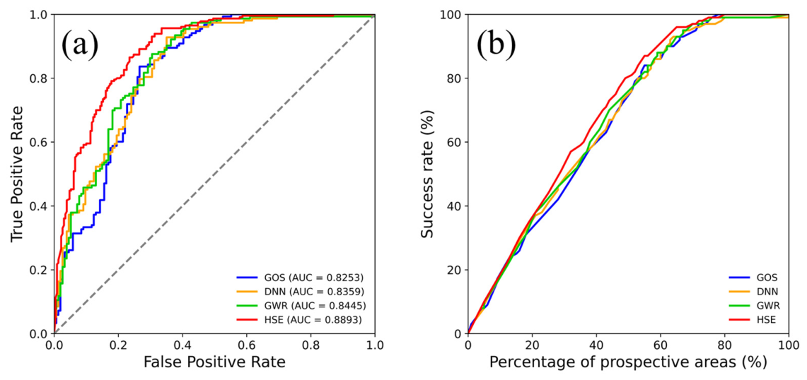
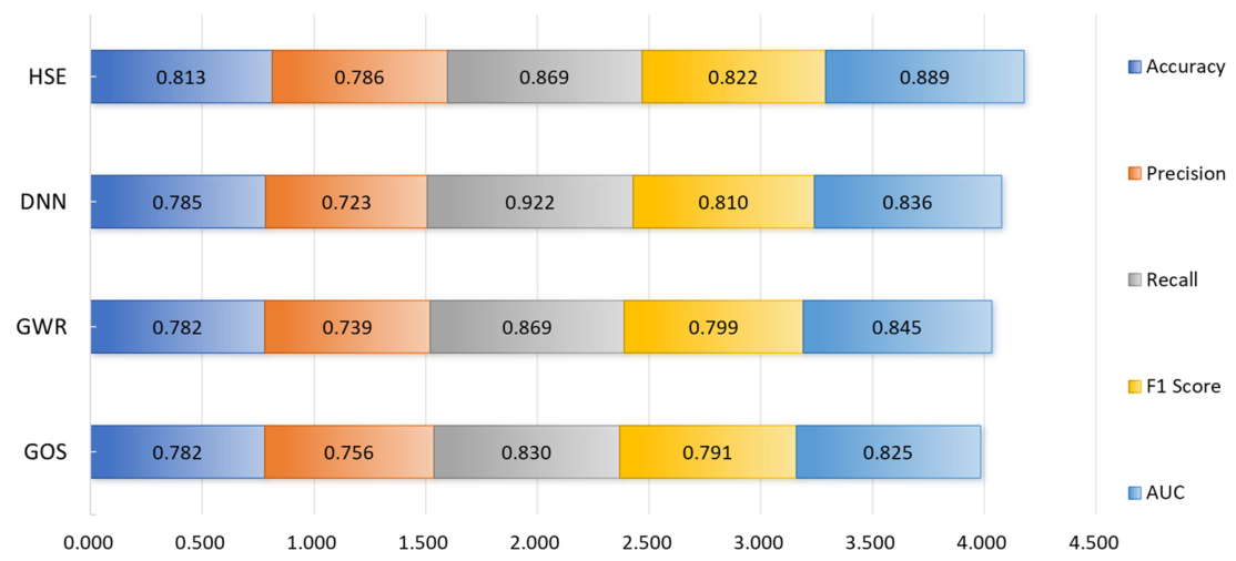
As illustrated in Figure 6 and Figure 7, the proposed HSE model achieved the best overall predictive performance among the compared models. Quantitatively, HSE obtained the highest Accuracy (0.813), Precision (0.786), F1-score (0.822), and AUC (0.889). Compared with the DNN model, which achieved an Accuracy of 0.785, Precision of 0.723, F1-score of 0.810, and AUC of 0.836, HSE improved the overall discriminative ability and prediction balance. In particular, the Precision of HSE increased by 0.063 in absolute terms relative to DNN, indicating a stronger ability to reduce false-positive landslide predictions.
It should be noted that DNN achieved the highest Recall (0.922), whereas the Recall of HSE was 0.869, corresponding to an absolute difference of 0.053, or 5.3 percentage points. Therefore, the advantage of HSE should not be interpreted as maximizing Recall alone. Instead, HSE provides a more balanced predictive performance, as reflected by its highest F1-score and AUC. This indicates that the proposed ensemble framework improves the trade-off between identifying true landslide occurrences and controlling false alarms.
This performance pattern is consistent with the role of the AICc-selected GWR bandwidth in controlling local model complexity. The selected adaptive bandwidth was 306 nearest training samples, indicating that the GWR component was calibrated at a moderately broad local spatial scale rather than at an overly localized scale. Such a bandwidth yields more regularized GWR probability outputs, which can reduce overly sensitive landslide labeling when these probabilities are fused by HSE. Consequently, HSE becomes less recall-oriented than DNN but achieves stronger false-alarm control and better overall discrimination, as reflected by its highest Precision, F1-score, and AUC. Therefore, the updated results are consistent with the theoretical purpose of AICc-based bandwidth selection, which is to balance local fit and model complexity rather than maximize sensitivity alone.
In contrast, the traditional spatial statistical models, GWR and GOS, showed more evident performance trade-offs. GWR achieved the same Recall as HSE (0.869), but its Accuracy (0.782), Precision (0.739), F1-score (0.799), and AUC (0.845) were lower than those of HSE, indicating weaker overall discriminative performance. GOS achieved a competitive Precision of 0.756, but it had the lowest Recall (0.830), F1-score (0.791), and AUC (0.825), suggesting that it tended to be more conservative in identifying landslide occurrences. Overall, these results demonstrate that HSE provides the most robust balance among discrimination ability, classification accuracy, landslide detection, and false-alarm control.
These results collectively confirm that the HSE model not only excels in overall predictive accuracy and discriminative ability but also maintains a well-balanced performance between correctly identifying landslide occurrences and reducing false alarms. The consistent and comprehensive improvements over the DNN baseline further validate that the proposed enhancements in the HSE framework effectively address the limitations of generic deep learning models in capturing the complex spatial and environmental dependencies inherent in landslide susceptibility assessment, leading to more reliable and robust predictions for practical landslide risk management.

3.3. Ablation Study

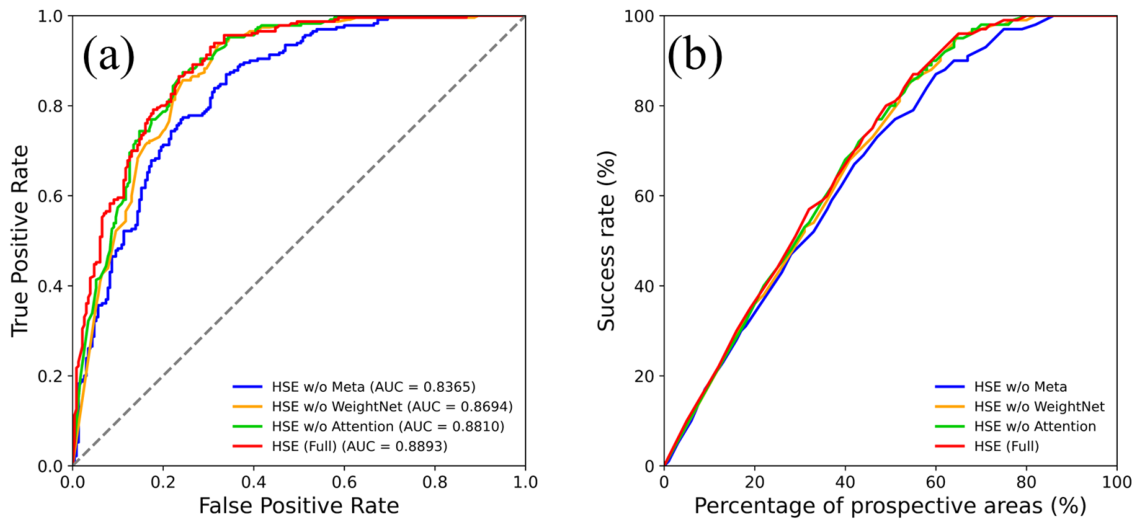
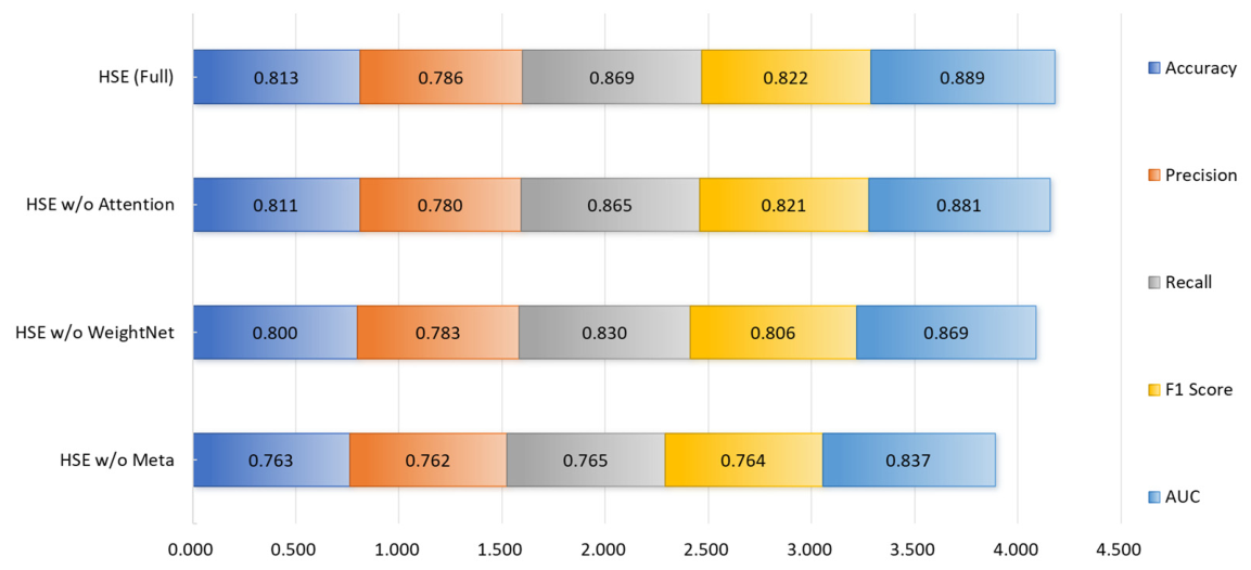
To rigorously validate the individual contributions of each core component in the proposed HSE framework, we conducted a systematic ablation study. Four model variants were constructed by sequentially removing the attention mechanism, the adaptive WeightNet module, and the meta-learner branch. The complete HSE (Full) model and its three ablated variants—HSE w/o Attention, HSE w/o WeightNet, and HSE w/o Meta—were evaluated across five metrics: accuracy, precision, recall, F1-score, and AUC. The results are presented in Figure 8 and Figure 9.
The full HSE model consistently outperforms all ablated variants across most metrics, achieving the highest accuracy (0.813), recall (0.869), F1-score (0.822), AUC (0.889), and a competitive precision of 0.786. These results demonstrate the synergistic benefits of integrating all three components for landslide susceptibility prediction.
Removing the meta-learner branch (HSE w/o Meta) causes the most pronounced performance degradation: accuracy declines to 0.763, AUC drops to 0.837, and F1-score falls to 0.764. This marked deterioration underscores the essential role of the meta-learner branch in integrating the probability outputs of GWR, GOS, and DNN. Without this branch, the ensemble network cannot fully exploit the complementary predictive evidence provided by the three base models, leading to reduced predictive accuracy and discriminative ability.
Eliminating the adaptive WeightNet module (HSE w/o WeightNet) also leads to notable performance reductions across all metrics, with accuracy, AUC, and F1-score decreasing to 0.800, 0.869, and 0.806, respectively. The WeightNet dynamically assigns sample-specific fusion weights to the three base models, allowing the ensemble to adaptively emphasize GWR, DNN, or GOS under different local geo-environmental contexts. Its removal forces the model to treat all input features equally, weakening its ability to capture meaningful, scale-dependent patterns in landslide susceptibility and thus compromising overall predictive robustness.
Disabling the spatial attention mechanism (HSE w/o Attention) yields a more nuanced performance pattern compared to the other ablations. While precision decreases marginally to 0.780 (compared to 0.786 for the full model), recall drops slightly to 0.865, resulting in a marginally lower F1-score (0.821) and AUC (0.881). These minor declines highlight the attention mechanism’s primary function: enhancing the model’s sensitivity to true landslide events by adaptively emphasizing informative feature representations and prediction embeddings. Without this mechanism, the model fails to leverage subtle spatial patterns indicative of landslide risk, leading to a minor increase in both false negatives and false positives, as reflected by the slight drops in recall and precision.
Collectively, these ablation results confirm that each component of the HSE framework fulfills a distinct, non-redundant role, and their integration yields complementary performance gains. The meta-learner branch addresses environmental heterogeneity, the WeightNet module optimizes feature utilization, and the attention mechanism enhances spatial context modeling. Only when all three modules are fully integrated does the model achieve the optimal balance of predictive accuracy, discriminative power, and practical utility for landslide susceptibility assessment, thereby validating the rationality and necessity of the proposed architectural design.

3.4. Spatial Distribution of Learned Base-Learner Weights

To further support the interpretability of the proposed HSE framework, we visualized the learned spatially varying weights assigned to the three base learners, namely GWR, DNN, and GOS. These weights were generated by the Softmax-normalized weight-generation module and therefore represent the relative contribution of each base learner at each sample location, rather than landslide susceptibility probabilities.
As shown in Figure 10 and Table 3, the learned weights exhibit clear spatial heterogeneity. The mean weights of GWR, DNN, and GOS are 0.345, 0.3347, and 0.3196, respectively, indicating that the HSE model does not rely on a single globally dominant learner. Meanwhile, the maximum weights of GWR, DNN, and GOS reach 0.9650, 0.9601, and 0.9500, respectively, suggesting that each base learner can provide the strongest local contribution under different spatial contexts. The relatively large standard deviations further indicate that the model adaptively adjusts base-learner contributions across space rather than assigning fixed global weights.
From a process perspective, high GWR weights indicate locations where local spatial non-stationarity contributes more strongly to susceptibility prediction, whereas high DNN weights reflect stronger reliance on nonlinear interactions among topographic, geological, hydrological, and anthropogenic factors. High GOS weights indicate areas where the similarity-based aggregation of environmentally similar samples provides stronger predictive information. Therefore, the learned weight maps provide spatially explicit diagnostic evidence of the adaptive ensemble process and support the interpretability of the proposed HSE framework.

3.5. Landslide Susceptibility Maps

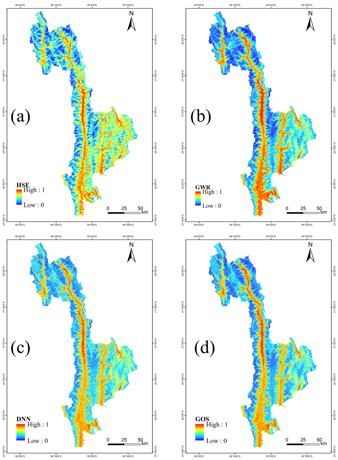
Following model training and inference, continuous landslide susceptibility indices (LSI) covering the entire study area were produced by the proposed HSE model as well as three comparative models, namely GWR, DNN, and GOS. To support practical hazard management and geomorphological interpretation, the continuous susceptibility surfaces were further categorized into five discrete levels—very low, low, moderate, high, and very high—using the Jenks Natural Breaks classification method. This approach is widely adopted in landslide susceptibility studies due to its ability to maximize between-class variance and minimize within-class variance [47], thereby generating geomorphologically meaningful zoning boundaries that align with the steep, highly dissected landscape of Nujiang Prefecture, Yunnan. As a typical high-mountain and steep-slope canyon region controlled by intense river incision and active tectonics, Nujiang exhibits strong spatial coupling between landslide distribution and topography [48,49], which provides a robust natural framework for validating the reasonability of model-derived susceptibility maps.
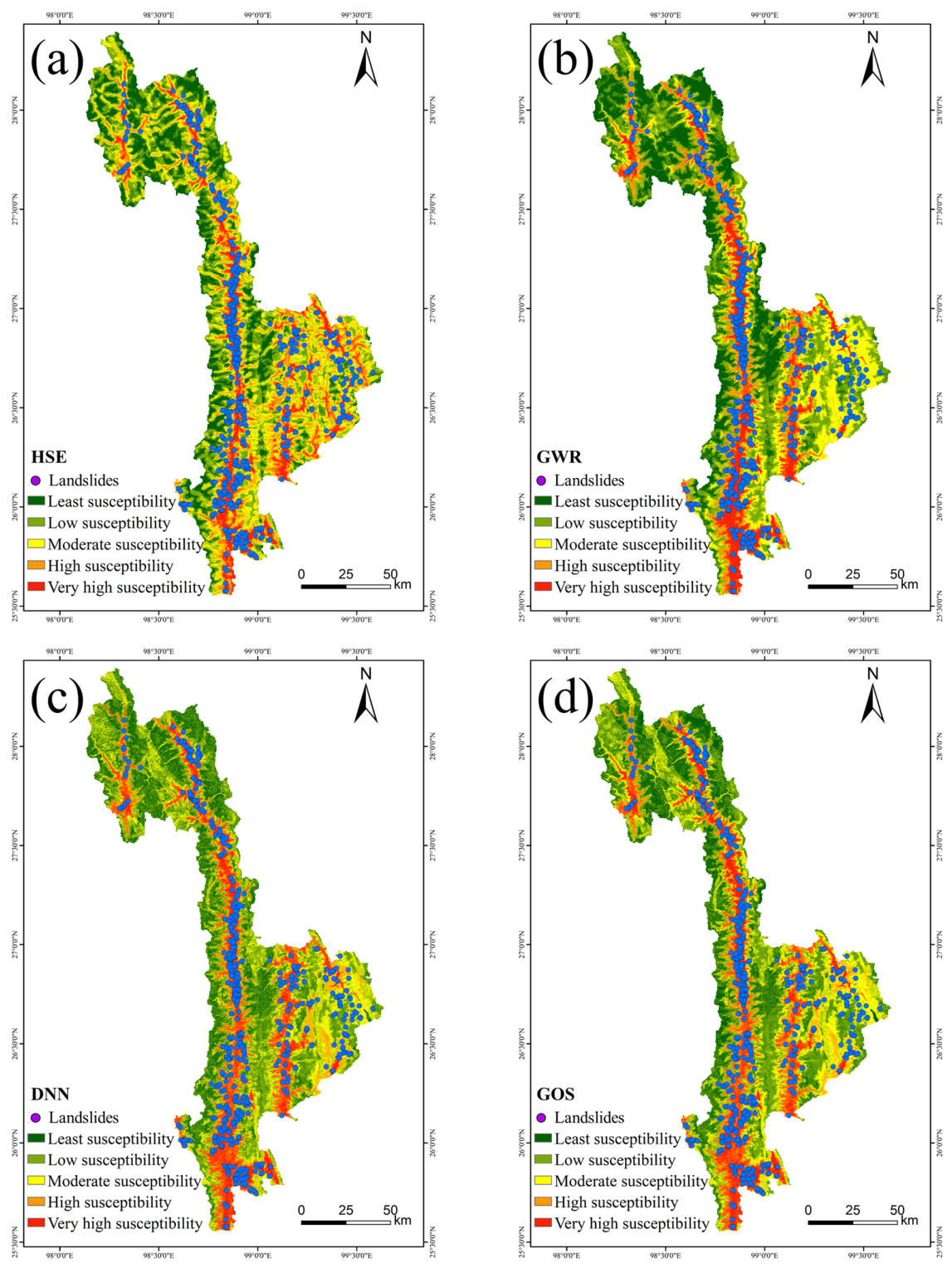
The spatial patterns of susceptibility zones obtained from all four models exhibit consistent and geologically plausible trends that conform to the regional geomorphic setting (Figure 11). High and very high susceptibility classes are predominantly distributed as narrow, continuous belts along the Nujiang River and its major tributaries, where steep channel slopes, prolonged fluvial undercutting, and loose colluvial deposits create favorable conditions for slope failures. In contrast, very low and low susceptibility zones are mainly concentrated in high-elevation watershed divides and gentle interfluve areas [50,51], where terrain gradients are mild, erosion intensity is weak, and landslide activity is rarely observed. This general spatial arrangement is consistent with the fundamental mechanism of landslide development in alpine canyon regions and confirms that all models effectively capture the first-order controls of topography on landslide occurrence.
To quantitatively evaluate the performance of each susceptibility zoning scheme, detailed statistical metrics—including area ratio, landslide count ratio, and landslide point density—were calculated for each susceptibility level and summarized in Table 4, Table 5, Table 6 and Table 7. Of the 561 mapped landslide points, 560 valid points fell within the classified susceptibility raster and were therefore used for zoning statistics. Across all models, landslide point density increases monotonically with rising susceptibility degree, verifying the logical consistency of the classification framework. The HSE model achieves notably more focused and efficient zoning than the three benchmark models. Its very high susceptibility zone accounts for only 13.15% of the total area but contains 63.39% of recorded landslide points, with an exceptionally high landslide density of 0.1835 points/km2. By comparison, the very high susceptibility zones of GWR, DNN, and GOS cover larger proportions of the study area (16.58%, 17.39%, and 16.67%, respectively) and yield considerably lower point densities (0.1555, 0.1506, and 0.1493 points/km2, respectively), indicating a tendency toward overestimation and spatially diffused high-risk delineation.
In combination with the unique high-mountain and steep-slope characteristics of Nujiang Prefecture, the zoning results of the HSE model demonstrate superior geomorphological rationality and practical applicability. The very low susceptibility class delineated by the HSE model, representing 17.12% of the region, contains no landslide points at all, and the low susceptibility zone contains merely 0.89% of landslides with a near-negligible density of 0.0013 points/km2; these zones correspond precisely to stable ridge tops and gentle interfluves where landslide occurrence is geomorphologically improbable. By contrast, the three comparative models misclassify certain moderately unstable slopes into low susceptibility zones, as reflected by higher landslide proportions within their low and very low classes. By integrating geospatial constraints and deep learning-based feature representation, the HSE model avoids excessive generalization of high-susceptibility areas and accurately identifies the narrow, steep riverine zones where landslide hazards are most concentrated. The resulting susceptibility map (Figure 12) thus provides a reliable, geologically consistent foundation for targeted landslide prevention, infrastructure planning, and land resource management in this hazard-prone alpine canyon region.

4. Discussion

4.1. Rationality of the Proposed HSE Framework

This study constructs a HSE framework paradigm that organically integrates spatial statistical models and deep learning for landslide susceptibility assessment. Single traditional spatial statistical methods (GWR and GOS) are good at capturing spatial non-stationarity of geo-environmental factors but lack the capability to characterize complex nonlinear interactions among multi-conditioning factors. A standalone DNN possesses strong nonlinear fitting capacity yet ignores inherent spatial topological dependencies and geographic prior constraints in geomorphological systems.
The designed ensemble architecture with dual-branch feature extraction, attention-driven adaptive fusion and dynamic weight allocation effectively bridges the gaps between spatial statistics and deep learning. As shown in Figure 10 and Table 3, the learned base-learner weights indicate that GWR, DNN, and GOS contribute differently across space rather than being assigned fixed global weights. Rather than simple model superposition, the framework incorporates geographic spatial knowledge into deep learning feature representation, which inherently adapts to the complex formation mechanism of landslides controlled by both structural geology and topographic heterogeneity in alpine canyon regions. After the base learners were independently trained and frozen, the attention-based ensemble network learned spatially adaptive fusion relationships among their prediction outputs, thereby improving both predictive robustness and model interpretability.

4.2. Inherent Mechanism of Performance Superiority

The performance divergence among models reflects their intrinsic adaptability to landslide evaluation scenarios. Traditional spatial statistical models exhibit obvious structural bias: they tend to trade off missing landslide events for higher precision or maintain moderate overall performance with insufficient discriminative capability, which limits their reliability in practical hazard prevention. The pure DNN baseline achieves competitive sensitivity but fails to balance precision and overall classification stability, easily producing biased prediction due to overfitting to local sample features.
By contrast, the HSE framework realizes a favorable trade-off between precision and recall. It suppresses false alarms caused by redundant noise factors and reduces the omission of potential landslide sites, which is highly consistent with the practical demand of landslide risk management that requires both avoiding blind early warning and identifying hidden dangers comprehensively. The performance advantage confirms that ensemble enhancement can effectively compensate the inherent defects of single models and strengthen the model’s ability to distinguish landslide and non-landslide units under complex geo-environmental backgrounds.

4.3. Functional Complementarity of Core Structural Components

The ablation analysis clarifies the independent positioning and synergistic effect of each key module in the HSE framework, without redundant functional overlap. The meta-learner branch acts as the basic support for cross-scenario generalization, enabling the model to learn generalized feature representations and adapt to spatially heterogeneous geological and geomorphic conditions. The WeightNet module realizes data-driven adaptive screening and weighting of conditioning factors, automatically highlighting dominant controlling factors and weakening the interference of irrelevant variables. The spatial attention mechanism focuses on capturing long-range spatial correlation among adjacent geographic units, excavating implicit spatial aggregation patterns of landslide distribution.
Each module undertakes a differentiated core function: addressing environmental heterogeneity, optimizing feature contribution, and strengthening spatial context modeling. Their organic integration forms a systematic enhancement effect, which explains why the complete HSE framework outperforms its ablated variants, and further verifies the scientificity and necessity of the proposed network architecture design.

4.4. Geomorphological Consistency and Application Implication of Susceptibility Mapping

All models can reflect the macroscopic spatial distribution rule of landslides in Nujiang Prefecture, with high-risk zones clustered along river valleys and low-risk zones distributed in stable watershed divides, which coincides with the regional geodynamic background dominated by river undercutting and tectonic activity [52,53]. Nevertheless, there exists essential difference in zoning refinement and geomorphological rationality.
Benefiting from the fusion of spatial constraint and deep learning feature mining, the HSE model produces more compact and reasonable susceptibility zoning [54]. It accurately confines high-hazard areas to narrow steep slope belts along rivers and perfectly matches low-susceptibility zones with stable gentle terrain, avoiding the over-diffusion of high-risk delineation and misclassification of stable geomorphic units commonly seen in benchmark models. The zoning results are geologically plausible and spatially targeted, which can provide refined decision support for regional landslide disaster prevention, infrastructure layout and territorial spatial planning [55].

5. Conclusions

This study proposed a hierarchical spatial adaptive ensemble (HSE) framework for landslide susceptibility mapping that explicitly addresses the fundamental challenge of spatial heterogeneity. The framework was validated on a typical landslide-prone catchment in Nujiang Prefecture, southwestern China. The findings lead to several important conclusions.
The HSE framework consistently outperforms the single-model baselines, including GWR, DNN, and GOS, in predictive accuracy, spatial consistency, and out-of-sample robustness. This superior performance is attributed to the attention-driven adaptive fusion mechanism, which learns spatially varying base-learner weights directly from environmental covariates and base predictions, thereby overcoming the fixed-weight and kernel-constrained limitations inherent in traditional ensemble methods.
The deliberate diversity of the three complementary base learners enables comprehensive characterization of landslide geospatial properties. Geographically weighted regression captures local spatial non-stationarity, the geographically optimal similarity model (grounded in the Third Law of Geography) quantifies local spatial autocorrelation, and the deep neural network mines nonlinear covariate interactions. No single learner excels across all geomorphic domains, but their attention-weighted combination adapts seamlessly to varying landscape conditions.
Spatial patterns of the resulting susceptibility maps are geomorphologically consistent: high-hazard zones are concentrated as narrow belts along the Nujiang River and its major tributaries, reflecting the dominant controls of fluvial undercutting and active tectonics, while low-hazard areas occupy stable interfluves and high-elevation divides. This alignment with regional geodynamic settings confirms that HSE produces physically plausible and spatially targeted susceptibility zoning.
Overall, these results demonstrate that explicitly learning spatial heterogeneity during ensemble fusion is not merely beneficial but essential for reliable landslide susceptibility mapping. One limitation is that the GOS component relies on the assumption that geo-environmentally similar locations tend to have similar landslide susceptibility, which was not independently validated as a stand-alone spatial-dependence hypothesis in the present study area. Future work will focus on integrating physical slope stability constraints and extending the framework to multi-temporal landslide assessment.

Author Contributions

Conceptualization, X.D. and Y.L.; methodology, X.D.; software, X.D.; validation, X.D.; formal analysis, X.D.; investigation, X.D.; data curation, X.D.; writing—original draft preparation, X.D.; visualization, X.D.; writing—review and editing, Y.L.; supervision, Y.L.; project administration, Y.L.; funding acquisition, Y.L. All authors have read and agreed to the published version of the manuscript.

Funding

This research was funded by Yunnan International Joint Laboratory of China-Laos-Bangladesh-Myanmar Natural Resources Remote Sensing Monitoring (202303AP140015); the key Project of Yunnan Science and Technology Department and Yunnan University Joint Fund (Grant No. 2019 FY003017); the National Natural Science Foundation of China (Grant No. 41161070) and the Geological Survey Project of China Geological Survey (Grant No. DD 20190545; Project of China Geological Survey (DD20221824).

Data Availability Statement

SRTM DEM (30 m) is available from NASA EarthData (https://earthdata.nasa.gov/). Landsat 8 OLI imagery is accessible via Geospatial Data Cloud (http://www.gscloud.cn/). Road network data are from the National Geomatics Center of China (http://www.ngcc.cn/). High-resolution Google Earth imagery was obtained from BIGEMAP (https://www.bigemap.com/). Historical landslide inventory, meteorological, fault, and lithology data were provided by local government agencies and are not publicly available due to institutional restrictions. All other derived data are available from the corresponding author upon reasonable request.

Acknowledgments

The authors extend their sincere thanks to the Earth Observation Team, BigeMap Download, China National Center of Surveying and Mapping, and geospatial Data Cloud, the research platform that provides vector data and image data. We acknowledge all people who contributed to the data collection and processing, as well as the constructive and insightful comments by the editor and anonymous reviewers.

Conflicts of Interest

The authors declare no conflicts of interest.

Abbreviations

The following abbreviations are used in this manuscript:
HSETwo-stage Hierarchical Spatial adaptive Ensemble framework
GWRGeographically Weighted Regression
DNNDeep Neural Network
GOSGeographically Optimal Similarity
LSMLandslide Susceptibility Mapping
LSILandslide Susceptibility Indices

References

  1. Schuster, R.L.; Fleming, R.W. Economic losses and fatalities due to landslides. Bull. Assoc. Eng. Geol. 1986, 23, 11–28. [Google Scholar] [CrossRef]
  2. Kirschbaum, D.B.; Adler, R.; Hong, Y.; Hill, S.; Lerner-Lam, A. A global landslide catalog for hazard applications: Method, results, and limitations. Nat. Hazards 2010, 52, 561–575. [Google Scholar] [CrossRef]
  3. Alexander, D. Vulnerability to landslides. In Landslide Hazard and Risk; John Wiley & Sons Ltd.: Hoboken, NJ, USA, 2005; pp. 175–198. [Google Scholar]
  4. Gerrard, J. The landslide hazard in the Himalayas: Geological control and human action. In Geomorphology and Natural Hazards; Elsevier: Amsterdam, The Netherlands, 1994; pp. 221–230. [Google Scholar]
  5. Shroder, J.F. Landslide Hazards, Risks, and Disasters; Elsevier: Amsterdam, The Netherlands, 2021. [Google Scholar]
  6. Crosta, G.; Clague, J. Dating, triggering, modelling, and hazard assessment of large landslides; landslides; engineering geology; geomorphology; hazard; monitoring. Geomorphology 2009, 103, 1–4. [Google Scholar] [CrossRef]
  7. Gariano, S.L.; Guzzetti, F. Landslides in a changing climate. Earth-Sci. Rev. 2016, 162, 227–252. [Google Scholar] [CrossRef]
  8. Ozturk, U.; Bozzolan, E.; Holcombe, E.A.; Shukla, R.; Pianosi, F.; Wagener, T. How climate change and unplanned urban sprawl bring more landslides. Nature 2022, 608, 262–265. [Google Scholar] [CrossRef] [PubMed]
  9. Duan, Y.; Ding, M.; He, Y. Global projections of future landslide susceptibility under climate change. Geosci. Front. 2025, 16, 102074. [Google Scholar] [CrossRef]
  10. Froude, M.J.; Petley, D.N. Global fatal landslide occurrence from 2004 to 2016. Nat. Hazards Earth Syst. Sci. 2018, 18, 2161–2181. [Google Scholar] [CrossRef]
  11. Haque, U.; Blum, P.; Da Silva, P.F.; Andersen, P.; Pilz, J.; Chalov, S.R.; Keellings, D. Fatal landslides in Europe. Landslides 2016, 13, 1545–1554. [Google Scholar] [CrossRef]
  12. Alcántara-Ayala, I. Landslides in a changing world. Landslides 2025, 22, 2851–2865. [Google Scholar] [CrossRef]
  13. Kirschbaum, D.; Kapnick, S.B.; Stanley, T.; Pascale, S. Changes in extreme precipitation and landslides over High Mountain Asia. Geophys. Res. Lett. 2020, 47, e2019GL085347. [Google Scholar] [CrossRef]
  14. Araújo, J.R.; Ramos, A.M.; Soares, P.M.; Melo, R.; Oliveira, S.C.; Trigo, R.M. Impact of extreme rainfall events on landslide activity in Portugal under climate change scenarios. Landslides 2022, 19, 2279–2293. [Google Scholar] [CrossRef]
  15. Debortoli, N.S.; Camarinha, P.I.M.; Marengo, J.A.; Rodrigues, R.R. An index of Brazil’s vulnerability to expected increases in natural flash flooding and landslide disasters in the context of climate change. Nat. Hazards 2017, 86, 557–582. [Google Scholar] [CrossRef]
  16. Guzzetti, F.; Mondini, A.C.; Cardinali, M.; Fiorucci, F.; Santangelo, M.; Chang, K.T. Landslide inventory maps: New tools for an old problem. Earth-Sci. Rev. 2012, 112, 42–66. [Google Scholar] [CrossRef]
  17. Reichenbach, P.; Rossi, M.; Malamud, B.D.; Mihir, M.; Guzzetti, F. A review of statistically-based landslide susceptibility models. Earth-Sci. Rev. 2018, 180, 60–91. [Google Scholar] [CrossRef]
  18. Corominas, J.; van Westen, C.; Frattini, P.; Cascini, L.; Malet, J.P.; Fotopoulou, S.; Smith, J.T. Recommendations for the quantitative analysis of landslide risk. Bull. Eng. Geol. Environ. 2014, 73, 209–263. [Google Scholar] [CrossRef]
  19. Fell, R.; Corominas, J.; Bonnard, C.; Cascini, L.; Leroi, E.; Savage, W.Z. JTC-1 Joint Technical Committee on Landslides and Engineered Slopes. Guidelines for landslide susceptibility, hazard and risk zoning for land use planning. Eng. Geol. 2008, 102, 85–98. [Google Scholar] [CrossRef]
  20. Chen, Y. Spatial prediction and mapping of landslide susceptibility using machine learning models. Nat. Hazards 2025, 121, 8367–8385. [Google Scholar] [CrossRef]
  21. Kudaibergenov, M.; Nurakynov, S.; Iskakov, B.; Iskaliyeva, G.; Maksum, Y.; Orynbassarova, E.; Sydyk, N. Application of artificial intelligence in landslide susceptibility assessment: Review of recent progress. Remote Sens. 2024, 17, 34. [Google Scholar] [CrossRef]
  22. Habib, M.; Habib, A.; Abboud, M. Multi-aspect critical assessment of applying digital elevation models in environmental hazard mapping. Rev. Int. Geomat. 2024, 33, 247–271. [Google Scholar] [CrossRef]
  23. Carrara, A.; Guzzetti, F.; Cardinali, M.; Reichenbach, P. Use of GIS technology in the prediction and monitoring of landslide hazard. Nat. Hazards 1999, 20, 117–135. [Google Scholar] [CrossRef]
  24. Dwivedi, D.; Poeppl, R.E.; Wohl, E. Hydrological connectivity: A review and emerging strategies for integrating measurement, modeling, and management. Front. Water 2025, 7, 1496199. [Google Scholar] [CrossRef]
  25. Carrara, A.; Cardinali, M.; Guzzetti, F.; Reichenbach, P. GIS technology in mapping landslide hazard. In Geographical Information Systems in Assessing Natural Hazards; Springer: Dordrecht, The Netherlands, 1995; pp. 135–175. [Google Scholar]
  26. Goetz, J.N.; Brenning, A.; Petschko, H.; Leopold, P. Evaluating machine learning and statistical prediction techniques for landslide susceptibility modeling. Comput. Geosci. 2015, 81, 1–11. [Google Scholar] [CrossRef]
  27. Huang, F.; Yin, K.; Huang, J.; Gui, L.; Wang, P. Landslide susceptibility mapping based on self-organizing-map network and extreme learning machine. Eng. Geol. 2017, 223, 11–22. [Google Scholar] [CrossRef]
  28. Liu, L.L.; Yang, C.; Wang, X.M. Landslide susceptibility assessment using feature selection-based machine learning models. Geomech. Eng. 2021, 25, 1–16. [Google Scholar]
  29. Gao, B.; He, Y.; Chen, X.; Chen, H.; Yang, W.; Zhang, L. A deep neural network framework for landslide susceptibility mapping by considering time-series rainfall. IEEE J. Sel. Top. Appl. Earth Obs. Remote Sens. 2024, 17, 5946–5969. [Google Scholar] [CrossRef]
  30. Habumugisha, J.M.; Chen, N.; Rahman, M.; Islam, M.M.; Ahmad, H.; Elbeltagi, A.; Dewan, A. Landslide susceptibility mapping with deep learning algorithms. Sustainability 2022, 14, 1734. [Google Scholar] [CrossRef]
  31. Azarafza, M.; Azarafza, M.; Akgün, H.; Atkinson, P.M.; Derakhshani, R. Deep learning-based landslide susceptibility mapping. Sci. Rep. 2021, 11, 24112. [Google Scholar] [CrossRef] [PubMed]
  32. Atkinson, P.M.; Massari, R. Autologistic modelling of susceptibility to landsliding in the Central Apennines, Italy. Geomorphology 2011, 130, 55–64. [Google Scholar] [CrossRef]
  33. Jiang, H.; Zhou, H.; Liu, M.; Wu, Y.; Guo, Y. Ensemble methods for landslide susceptibility mapping: A review of machine learning and hybrid approaches. Carbonates Evaporites 2025, 41, 16. [Google Scholar] [CrossRef]
  34. Lü, G.; Batty, M.; Strobl, J.; Lin, H.; Zhu, A.X.; Chen, M. Reflections and speculations on the progress in Geographic Information Systems (GIS): A geographic perspective. Int. J. Geogr. Inf. Sci. 2019, 33, 346–367. [Google Scholar] [CrossRef]
  35. Utomo, W.Y.; Anwar, S.; Tarigan, S.D.; Barus, B. Carbon Stock Assessment and Estimation Using Machine Learning: A Case Study on Acacia Forest Plantation in Rupat Island Peat Ecosystem, Indonesia. Environ. Chall. 2026, 23, 101518. [Google Scholar] [CrossRef]
  36. Dietterich, T.G. Ensemble methods in machine learning. In International Workshop on Multiple Classifier Systems; Springer: Berlin/Heidelberg, Germany, 2000; pp. 1–15. [Google Scholar]
  37. Di Napoli, M.; Carotenuto, F.; Cevasco, A.; Confuorto, P.; Di Martire, D.; Firpo, M.; Calcaterra, D. Machine learning ensemble modelling as a tool to improve landslide susceptibility mapping reliability. Landslides 2020, 17, 1897–1914. [Google Scholar] [CrossRef]
  38. Fang, Z.; Wang, Y.; Peng, L.; Hong, H. A comparative study of heterogeneous ensemble-learning techniques for landslide susceptibility mapping. Int. J. Geogr. Inf. Sci. 2021, 35, 321–347. [Google Scholar] [CrossRef]
  39. Kadavi, P.R.; Lee, C.W.; Lee, S. Application of ensemble-based machine learning models to landslide susceptibility mapping. Remote Sens. 2018, 10, 1252. [Google Scholar] [CrossRef]
  40. Wei, A.; Yu, K.; Dai, F.; Gu, F.; Zhang, W.; Liu, Y. Application of tree-based ensemble models to landslide susceptibility mapping: A comparative study. Sustainability 2022, 14, 6330. [Google Scholar] [CrossRef]
  41. Clark, M.K.; Royden, L.H. Topographic ooze: Building the eastern margin of Tibet by lower crustal flow. Geology 2000, 28, 703–706. [Google Scholar] [CrossRef]
  42. Burchfiel, B.C.; Wang, E. Northwest-trending, middle Cenozoic, left-lateral faults in southern Yunnan, China, and their tectonic significance. J. Struct. Geol. 2003, 25, 781–792. [Google Scholar] [CrossRef]
  43. Brunsdon, C.; Fotheringham, S.; Charlton, M. Geographically weighted regression. J. R. Stat. Soc. Ser. D (Stat.) 1998, 47, 431–443. [Google Scholar] [CrossRef]
  44. Sze, V.; Chen, Y.H.; Yang, T.J.; Emer, J.S. Efficient processing of deep neural networks: A tutorial and survey. Proc. IEEE 2017, 105, 2295–2329. [Google Scholar] [CrossRef]
  45. Song, Y. Geographically optimal similarity. Math. Geosci. 2023, 55, 295–320. [Google Scholar] [CrossRef]
  46. Ran, T.; Xu, R.G.; Song, Y.P.; He, K.; Qing, Y.D.; Li, Q. Development characteristics and sensitivity analysis of impact factors of slope geohazards in Chawalong–Gongshan section of Nujiang River basin. Geol. Bull. China 2026. [Google Scholar] [CrossRef]
  47. Kumar, R.; Anbalagan, R. Landslide susceptibility mapping using analytical hierarchy process (AHP) in Tehri reservoir rim region, Uttarakhand. J. Geol. Soc. India 2016, 87, 271–286. [Google Scholar] [CrossRef]
  48. Shang, Y.; Park, H.D.; Yang, Z.; Yang, J. Distribution of landslides adjacent to the northern side of the Yarlu Tsangpo Grand Canyon in Tibet, China. Environ. Geol. 2005, 48, 721–741. [Google Scholar] [CrossRef]
  49. Yang, Z.; Pang, B.; Dong, W.; Li, D.; Huang, Z. Interaction of landslide spatial patterns and river canyon landforms: Insights into the Three Parallel Rivers Area, southeastern Tibetan Plateau. Sci. Total Environ. 2024, 914, 169935. [Google Scholar] [CrossRef]
  50. Zang, Y.Q.; Guo, Y.G.; Su, L.B.; Wang, G.W.; Wu, S.J.; Qin, D.S. Study on multi-model evaluation methods for landslide susceptibility in southeastern Tibet. Chin. J. Geol. Hazard Control 2024, 35, 58–69. [Google Scholar]
  51. Wang, S.; Ling, S.; Wu, X.; Wen, H.; Huang, J.; Wang, F.; Sun, C. Key predisposing factors and susceptibility assessment of landslides along the Yunnan–Tibet traffic corridor, Tibetan plateau: Comparison with the LR, RF, NB, and MLP techniques. Front. Earth Sci. 2023, 10, 1100363. [Google Scholar] [CrossRef]
  52. Shen, X.; Tian, Y.; Wang, Y.; Wu, L.; Jia, Y.; Tang, X.; Liu-Zeng, J. Enhanced quaternary exhumation in the central three rivers region, southeastern Tibet. Front. Earth Sci. 2021, 9, 741491. [Google Scholar] [CrossRef]
  53. Chen, L.; Wang, P.; Cao, X.; Zhang, H. Numerical modeling of landscape and drainage evolution in the southeastern Tibetan Plateau since 50 Ma. Quat. Sci. 2025, 45, 1039–1054. [Google Scholar]
  54. Zeng, T.; Wu, L.; Hayakawa, Y.S.; Yin, K.; Gui, L.; Jin, B.; Peduto, D. Advanced integration of ensemble learning and MT-InSAR for enhanced slow-moving landslide susceptibility zoning. Eng. Geol. 2024, 331, 107436. [Google Scholar] [CrossRef]
  55. Moldovan, C.; Roșca, S.; Dolean, B.; Rusu, R.; Ursu, C.D.; Man, T. Spatial planning decision based on geomorphic natural hazards distribution analysis in Cluj County, Romania. Appl. Sci. 2024, 14, 440. [Google Scholar] [CrossRef]
Figure 1. Geographic location of the study area (Nujiang Prefecture, Yunnan, China).
Remotesensing 18 01999 g001
Figure 2. Environmental conditioning factors for landslide susceptibility modeling in the study area: (a) elevation; (b) slope; (c) aspect; (d) proximity to roads; (e) proximity to rivers; (f) proximity to faults; (g) precipitation; (h) NDVI; (i) lithology.
Remotesensing 18 01999 g002
Figure 3. Overall workflow of the proposed HSE framework for landslide susceptibility mapping.
Remotesensing 18 01999 g003
Figure 4. Schematic architecture of the proposed HSE framework. The framework integrates three base learners (GWR, GOS, and DNN), followed by multi-scale feature extraction, adaptive attention-based feature fusion, and dynamic weight generation, to produce the final landslide susceptibility prediction.
Remotesensing 18 01999 g004
Figure 5. Sensitivity analysis of the GOS κ parameter with ±0.1 variation. Performance comparison of the GOS model under κ = 0.1, 0.2, and 0.3 using (a) ROC curves and (b) success-rate curves.
Remotesensing 18 01999 g005
Figure 6. Comparison of models (GOS, DNN, GWR, and HSE): (a) ROC curves, (b) success-rate curves.
Remotesensing 18 01999 g006
Figure 7. Performance comparison of the proposed HSE model and benchmark models (GOS, GWR, and DNN) using accuracy, precision, recall, F1-score, and AUC metrics.
Remotesensing 18 01999 g007
Figure 8. Ablation study results: performance comparison of the full HSE model and its ablated variants using (a) ROC curves and (b) success-rate curves.
Remotesensing 18 01999 g008
Figure 9. Performance comparison of the full HSE model and its ablated variants using accuracy, precision, recall, F1-score, and AUC metrics.
Remotesensing 18 01999 g009
Figure 10. Spatial distribution of learned base-learner weights in the HSE model: (a) GWR weight, (b) DNN weight, and (c) GOS weight.
Remotesensing 18 01999 g010
Figure 11. Landslide Susceptibility Index (LSI) maps produced by different models: (a) HSE, (b) GWR, (c) DNN, and (d) GOS.
Remotesensing 18 01999 g011
Figure 12. Classified landslide susceptibility zoning maps from different models: (a) HSE, (b) GWR, (c) DNN, and (d) GOS.
Remotesensing 18 01999 g012
Table 1. Source for the landslide conditioning factors used in this study.
Data CategoryDataset NameSource
Remote Sensing ImageryLandsat 8 OLI ImageryGeospatial Data Cloud (http://www.gscloud.cn/, accessed on 15 March 2025)
Google Earth Remote Sensing ImageryBIGEMAP Mapping Platform
Basic Geographic & Thematic DataHistorical Landslide Inventory DataNujiang Prefecture Bureau of Natural Resources and Planning
Meteorological DataNujiang Prefecture Meteorological Bureau and Water Affairs Bureau
Drainage Network DataExtracted from SRTM DEM Dataset
Road Network DataNational Geomatics Center of China (http://www.ngcc.cn/, accessed on 18 March 2025)
NDVI DataDerived from Landsat 8 OLI Imagery
Fault DataExtracted from 1:250,000-scale geological maps (Nujiang Prefecture Bureau of Natural Resources and Planning)
Lithology DataExtracted from 1:250,000-scale geological maps (Nujiang Prefecture Bureau of Natural Resources and Planning)
Table 2. CF values of conditioning-factor classes used for initial CF-based landslide susceptibility mapping and non-landslide sample construction.
FactorClassificationArea (km2)Number of Landslide PointsCF
Elevation (m)<1200253.4256250.6375
1200~1600695.91511180.8057
1600~1900985.47661620.7984
1900~24002467.76221870.5162
2400~30004342.702567−0.6050
3000~36003874.66382−0.9870
>36002083.05420−1.0000
Slope (°)0°~10°731.0079300.0731
10°~20°2240.54281160.2735
20°~30°3820.08151870.2293
30°~40°4425.603153−0.0973
40°~50°2680.715763−0.3933
>50°805.049112−0.6186
AspectPlane22.22550−1.0000
North1886.000440−0.4538
Northeast1702.0764680.0467
East1852.4251000.3048
Southeast1806.8571750.084
South1907.382656−0.2375
Southwest1849.515966−0.0671
West1862.0028960.2703
Northwest1814.514360−0.1379
Proximity to rivers (m)0~2001610.7471940.3599
200~4001539.69211190.5264
400~6001476.4599840.3424
600~8001412.6364900.417
800~10001348.4016660.2292
1000~12001273.5279510.0491
>12006041.53557−0.7599
LithologyWeak rock group7073.2944230−0.1528
Hard rock group4066.362148−0.0479
Harder rock group3545.01871830.2712
Loose rock group18.32490−1.0000
Proximity to faults (m)<4001764.5994940.295
400~8001569.76561190.5164
800~12001359.7416840.3975
1200~16001274.3034900.478
1600~2000999.117660.4392
2000~2400844.9938510.3824
>24006890.479257−0.7897
NDVIPoor289.26550−1.0000
Average980.598921−0.4483
Good3216.5431102−0.1744
Excellent5367.60632450.1706
Very excellent4832.63261930.0464
Proximity to roads (m)0~2001753.14962750.7868
200–4001560.81151000.4205
400~6001390.594545−0.1570
600~8001249.389933−0.3161
800~10001111.776329−0.3248
1000~12001087.854931−0.2606
1200~1400863.120718−0.4631
>14005686.302630−0.8663
Precipitation (mm)852~10214331.93672070.2095
1021~11523233.56861310.0605
1152~12992430.362450−0.4705
1299~14512797.7581300.2284
1451~16561909.374343−0.4192
Table 3. Summary statistics of learned base-learner weights in the HSE model.
Base LearnerMean WeightStd.Min.Max.
GWR0.34560.39890.01530.9650
DNN0.33470.38610.01860.9601
GOS0.31960.40110.00720.9500
Table 4. Statistical table of HSE model susceptibility.
Degree of SusceptibilityArea (km2)Ratio (%)Number of Disasters (Unit)Ratio(%)Disaster Point Density (Unit/km2)
Very low2517.3317.12%000.0000
Low3711.2425.24%50.89%0.0013
Moderate3558.1524.20%468.21%0.0129
High2981.8620.28%15427.50%0.0516
Very high1934.4213.15%35563.39%0.1835
Table 5. Statistical table of GWR model susceptibility.
Degree of SusceptibilityArea (km2)Ratio (%)Number of Disasters (Unit)Ratio (%)Disaster Point Density (Unit/km2)
Very low3110.8621.16%000
Low4190.4528.50%61.07%0.0014
Moderate2950.4220.07%6010.71%0.0203
High2013.3713.69%11520.54%0.0571
Very high2437.9016.58%37967.68%0.1555
Table 6. Statistical table of DNN model susceptibility.
Degree of SusceptibilityArea (km2)Ratio (%)Number of Disasters (Unit)Ratio (%)Disaster Point Density (Unit/km2)
Very low2603.3417.71%000.0000
Low4393.6529.88%101.79%0.0023
Moderate3075.6220.92%508.93%0.0163
High2073.9314.11%11520.54%0.0555
Very high2556.4617.39%38568.75%0.1506
Table 7. Statistical table of GOS model susceptibility.
Degree of SusceptibilityArea (km2)Ratio (%)Number of Disasters (Unit)Ratio (%)Disaster Point Density (Unit/km2)
Very low2595.3217.65%000.0000
Low4263.2129.00%91.61%0.0021
Moderate3136.6121.33%498.75%0.0156
High2256.8415.35%13624.29%0.0603
Very high2451.0216.67%36665.36%0.1493
Disclaimer/Publisher’s Note: The statements, opinions and data contained in all publications are solely those of the individual author(s) and contributor(s) and not of MDPI and/or the editor(s). MDPI and/or the editor(s) disclaim responsibility for any injury to people or property resulting from any ideas, methods, instructions or products referred to in the content.