WildfireCube: A Dense Spatiotemporal Tensor to Support Multi-Regime Wildfire Spread Modeling at 30 m/3 h Resolution

Highlights

What are the main findings?

• A reproducible pipeline assembles dense (T, C, H, W) wildfire tensors at 30 m/3 h resolution from four open remote-sensing sources, covering several events.
• Physics-informed normalization with fixed physical bounds (not sample statistics) enables cross-event transfer and exact inversion to physical units.
• A dataset that enables the training of neural networks framing the wildfire spread as a spatiotemporal problem.

What are the implications of the main findings?

• The causal channel structure (static landscape, dynamic weather, evolving fire state) directly supports teacher-forced autoregressive training of spatiotemporal neural networks.
• Zarr-based chunked storage with additional Zstandard compression reduces on-disk footprint by over 60%, enabling the full multi-event catalog to be hosted on commodity storage, enabling wider availability for experimentation.

Abstract

Machine learning approaches to wildfire spread prediction are constrained by the lack of standardized, multi-source, spatiotemporal datasets that fuse terrain, weather, and fire-state information into a single ML-ready format. We present WildfireCube, a reproducible event-centric pipeline and methodology for constructing dense fourth-order spatiotemporal tensors of shape (T, C, H, W) at 30 m spatial and 3 h temporal resolution. Following the analysis-ready data convention established in the Earth Observation community, the pipeline fuses four open data sources: the Copernicus GLO-30 Digital Elevation Model for static terrain derivatives, ERA5-Land reanalysis for hourly weather forcing, Sentinel-2 Level-2A imagery for spectral vegetation and burn-severity indices, and NASA FIRMS active-fire hotspot detections for fire-state reconstruction via ordinary kriging. The resulting 13-channel normalized tensor separates causal drivers into three physically motivated groups: static landscape controls (elevation, slope, aspect, fuel load), dynamic atmospheric forcings (wind components, temperature, precipitation), and evolving fire state (fire-front mask, burn severity, fractional burn, observation confidence). A physics-informed normalization framework maps all channels to bounded ranges using fixed physical constants rather than sample statistics, ensuring cross-event comparability and exact invertibility. We demonstrate the pipeline on 13 wildfire events across the United States, Canada, and Greece (2017–2023), producing a processed catalog exceeding 300 GB compressed and spanning a 14-fold range in burned area, a 27 °C range in mean temperature, and different fire regimes. Event tensors are stored in chunked Zarr archives with Zstandard compression, achieving a 2.58× compression ratio. As future work, the pipeline will be applied to a 40-event target catalog projected to exceed 2 TB of raw data, providing the multi-regime diversity and scale required for training robust deep learning models for spatiotemporal wildfire prediction.

1. Introduction

Wildfire frequency and severity have escalated markedly over the past two decades, driven by the compounding effects of climate change, prolonged drought regimes, and expanding wildland–urban interfaces. The 2021 Dixie Fire in California consumed over 3900 km²; the 2023 Canadian boreal season burned an unprecedented 18.5 million hectares; and Mediterranean Europe experienced record fire seasons in 2021 and 2023. These trends are symptoms of a global shift in fire weather, fuel dryness, and ignition patterns that demand fundamentally improved prediction capabilities.

Machine learning has emerged as a promising avenue for wildfire spread forecasting, with architectures ranging from convolutional sequence models to graph neural networks demonstrating skill on individual fire events [1]. Beyond remote sensing data, machine learning and large language models have also been applied to social media analysis for wildfire and disaster situational awareness, enabling complementary approaches for damage assessment and post-event response [2,3]. Yet a persistent bottleneck constrains progress: the absence of standardized, multi-source, spatiotemporal datasets that fuse terrain, weather, and fire-state information into a single ML-ready format. Existing benchmarks rely on coarse-resolution gridded products, single-source observations, or hand-curated feature sets that conflate the causal structure of fire behavior. Without a common data representation that preserves physical units, spatial alignment, and temporal coherence, it is difficult to compare models across fire regimes, reproduce experimental results, or transfer learned representations across geographic contexts.

Wildfire spread is governed by three distinct classes of physical drivers: the static landscape over which fire propagates (terrain morphology, fuel structure), the dynamic atmospheric forcing that modulates the rate of spread (wind speed and direction, temperature, precipitation), and the evolving fire state itself (the current burn perimeter, severity, and observational certainty). Any dataset that collapses these classes into undifferentiated feature vectors obscures the causal mechanisms that physically interpretable models must learn.

1.1. Tensor Representation and Terminology

This work presents WildfireCube: a reproducible, event-centric pipeline and methodology for constructing dense fourth-order spatiotemporal tensors of shape (T, C, H, W), where T indexes temporal bins, C indexes data channels, and H × W spans a georeferenced spatial grid at 30 m resolution and 3 h temporal resolution. From the perspective of linear algebra and machine learning, the (T, C, H, W) data structure is formally a fourth-order tensor, and we adopt this terminology throughout. The product name “WildfireCube” follows the analysis-ready data cube (ARD) convention established in the Earth Observation community, used, for example, by the Open Data Cube initiative, the Copernicus Data Space Ecosystem, and the Sentinel Hub processing API—where “data cube” refers to multi-dimensional raster arrays organized along spatial, temporal, and spectral axes. The two terminologies are complementary: “tensor” is precise when specifying the mathematical object and its ML use, and “data cube” situates the work within the geospatial ARD literature and signals interoperability with geospatial tooling.

The cube structure operationalizes wildfire as a discrete-time dynamical system. At each temporal transition, the next fire state is determined by the current fire state, incoming weather forcing, and the fixed landscape:

Y_t+1 = F(Y_t, D_t+1, S)

(1)

where Y_t encodes the fire state at time t, D_t+1 the incoming weather forcings over the interval (t, t + 1], and S the static landscape. This formulation separates causal structure into three physically interpretable argument classes consistent with established wildfire science. During training, the ground-truth Y_t is provided at each step (teacher forcing); during inference, the model’s own prediction is fed back autoregressively.

1.2. Event Catalog Overview

To demonstrate the pipeline, we process 13 wildfire events spanning three countries (United States, Canada, and Greece) over the period of 2017–2023. These 13 events are drawn from a broader events target catalog deliberately constructed to cover diverse fire regimes, terrain types, and climate zones: Mediterranean shrubland and maquis (Evia 2021, Rhodes 2023, Evros 2023, Varnavas 2024), boreal and sub-boreal conifer (Horse River 2016, Elephant Hill 2017, Chuckegg Creek 2019, McDougall Creek 2023, Jasper 2024), montane and alpine (Cameron Peak 2020, East Troublesome 2020, Cedar Creek 2022, Bootleg 2021), California chaparral and mixed conifer (Soberanes 2016, Thomas 2017, Carr 2018, Creek 2020, Dixie 2021, Mosquito 2022, Lake 2024, Park 2024), wind-driven extreme events (Lahaina 2023), and sub-arctic tundra–boreal transition (Swan Lake 2019). Processing the remaining events to complete the full catalog is planned as immediate future work, producing a large-scale dataset suitable for training deep learning models.

1.3. Principal Contributions

The principal contributions of this work are: (1) a fully reproducible, event-centric pipeline in which each fire is specified by a single YAML configuration file and processed end-to-end without manual intervention; (2) a standardized, ML-ready data representation that encodes wildfire events as dense (T, C, H, W) tensors with physically meaningful channels; (3) a causally structured channel layout that separates static controls, dynamic forcings, and fire state into distinct groups supporting teacher-forced autoregressive training; (4) a physics-informed normalization framework that maps all channels to comparable numeric ranges using domain-specific bounds rather than sample statistics; and (5) a demonstration of the pipeline on 13 events across three countries and six fire regimes.

2. Related Work

This section situates WildfireCube within the rapidly evolving landscape of wildfire machine learning datasets, fire arrival-time reconstruction methods, burn severity mapping, fire weather reanalysis, and the broader Earth System Data Cube paradigm. We identify key advances and remaining gaps that motivate the design choices described in subsequent sections.

2.1. Wildfire ML Datasets and Benchmarks

The growth of machine learning for wildfire prediction has been accompanied by a parallel effort to construct standardized, benchmark-ready datasets. Huot et al. [4] introduced the Next Day Wildfire Spread dataset, aggregating nearly a decade of US wildfire data via Google Earth Engine into 64 × 64 pixel grids at 1 km spatial and daily temporal resolution. This dataset pairs MODIS fire detections with topography, vegetation (NDVI), weather (GridMET), drought indices, and population density, framing fire spread as binary image segmentation. It has become the de facto benchmark, yet its coarse resolution limits the representation of fine-scale fire behavior such as spotting, terrain-channeled runs, and diurnal spread cycles.

Gerard et al. [5] advanced the temporal dimension with WildfireSpreadTS, providing 13,607 images across 607 US fire events (2018–2021) at 375 m spatial and 24 h temporal resolution with 23 input channels. Their benchmarks demonstrated that models incorporating multi-temporal context (3–5 preceding days) significantly outperform single-image baselines, with ConvLSTM achieving 8–12% F1 improvement. Kondylatos et al. [6] constructed Mesogeos, a Mediterranean-focused datacube at 1 km and daily resolution spanning 17 years (2006–2022), integrating ERA5-Land meteorology, MODIS vegetation, and topography. Their deep learning baselines significantly outperformed traditional approaches for wildfire danger prediction. Papakis et al. [7] developed a multimodal ensemble deep learning model for wildfire prediction in Greece, fusing satellite imagery (NDVI), meteorological observations, and topographic features from 2017 to 2021 through an ensemble of CNNs and MLPs that achieved 96.15% classification accuracy, demonstrating the value of multi-source data fusion for Mediterranean wildfire prediction. At global scale, Karasante et al. [8] released SeasFire, a 59-variable Zarr-based cube at 0.25 degree and 8-day resolution for sub-seasonal wildfire forecasting. These datasets collectively establish the datacube paradigm for wildfire ML but operate at spatial resolutions (375 m to 0.25 degree) and temporal cadences (daily to 8 days) that cannot resolve the sub-daily, sub-kilometer dynamics central to operational fire management.

2.2. Fire Arrival-Time Reconstruction

Reconstructing continuous fire arrival-time surfaces from discrete satellite detections is fundamental to building temporally resolved fire progression tensors. Barber et al. [9] produced the Canadian Fire Spread Dataset (CFSDS), applying ordinary kriging to MODIS and VIIRS thermal anomalies to generate day-of-burning surfaces for 3269 fires across forested Canada (2002–2021). Validation against provincial agency perimeters yielded Sørensen–Dice coefficients generally exceeding 0.7. The CFSDS operates at 180 m spatial and daily temporal resolution, pairing kriged fire progression with ERA5-Land weather covariates and forest fuel characteristics. WildfireCube adopts the same geostatistical interpolation framework but extends it to 30 m spatial and 3 h temporal resolution, enabling reconstruction of sub-daily fire dynamics invisible at the daily scale.

Farguell et al. [10] proposed a support vector machine approach for estimating fire arrival time from MODIS/VIIRS Level-2 active-fire data. Tested on the 10 largest California wildfires of 2020, the method achieved 12% mean absolute percentage error in burned area and a 0.82 average Sørensen coefficient against independent airborne infrared perimeters. Chen et al. [11] took an alternative object-tracking approach with the Fire Event Data Suite (FEDS), mapping California wildfire progression (2012–2020) at half-daily timesteps by spatially clustering and temporally appending VIIRS 375 m active-fire detections to tracked fire objects. These complementary methodologies highlight a spectrum of approaches from geostatistical interpolation (kriging) through ML-based estimation to object-level tracking, with WildfireCube positioned at the high-resolution end of the geostatistical branch.

2.3. Burn Severity and Sentinel-2 Remote Sensing

Sentinel-2 multispectral imagery has become the standard for high-resolution burn severity mapping. Sdraka et al. [12] presented FLOGA, a comprehensive ML-ready dataset for Greece comprising pre- and post-fire Sentinel-2 and MODIS imagery for 326 wildfire events (2017–2021) with expert-annotated burned area ground truth at 10 m resolution. Their benchmarks demonstrated that Sentinel-2 shortwave infrared bands (B11, B12) and derived indices (dNBR, RBR) were the most discriminative features for burn detection, with the novel BAM-CD model achieving an IoU of 0.79 through joint encoding of bi-temporal Sentinel-2 pairs. WildfireCube leverages these same spectral indices, computing the Relativized Burn Ratio from pre- and post-fire Sentinel-2 composites as its severity channel.

Fuel moisture content is a critical but challenging variable for wildfire modeling. Rao et al. [13] demonstrated that combining Sentinel-1 SAR backscatter with Landsat-8 optical reflectance through a physics-assisted recurrent neural network improves live fuel moisture estimation substantially (R-squared from 0.44 optical-only to 0.63 with SAR), revealing that microwave sensitivity captures moisture dynamics invisible to NDVI alone. WildfireCube currently uses NDVI as a proxy for fuel load; the integration of SAR-derived fuel moisture represents a natural future extension.

2.4. Fire Weather and ERA5 Reanalysis

ERA5 and its land-surface variant ERA5-Land have become the standard meteorological forcing for wildfire ML applications. Vitolo et al. [14] produced the foundational ERA5-based global fire weather danger maps, demonstrating that ERA5-derived Fire Weather Index values correlate significantly better with observed fire activity than the predecessor ERA-Interim product. Kondylatos et al. [15] constructed a 1 km datacube with 90 ERA5-Land variables for wildfire danger prediction in Greece, where explainable AI analysis identified soil moisture deficit and low relative humidity as the primary fire danger drivers, challenging the common assumption that temperature is the dominant predictor.

At global scale, Di Giuseppe et al. [16] demonstrated in Nature Communications that ML models trained on curated multi-source data reduce the false-alarm rate of fire danger forecasts by 30–50% compared to traditional FWI-based approaches. A key finding was that data quality and resolution proved more important than model complexity, with simpler models on better-curated inputs matching or outperforming deep learning on noisier data. This result directly validates the investment in high-resolution, physics-normalized data curation that underpins WildfireCube.

2.5. Earth System Data Cubes and Cloud-Native Infrastructure

WildfireCube belongs to the broader family of Earth System Data Cubes (ESDCs). Montero et al. [17] provide the definitive survey of the ESDC paradigm, covering the full lifecycle from data ingestion and spatiotemporal alignment through cloud-native storage to ML applications. They report that ESDC-structured data reduces preprocessing overhead by 60–80% for downstream ML tasks and advocate for cloud-native formats such as Zarr and Cloud-Optimized GeoTIFF. Ji et al. [18] exemplify this approach with DeepExtremeCubes, fusing the same data sources as WildfireCube (Sentinel-2 L2A imagery and ERA5-Land reanalysis) into over 40,000 globally sampled minicubes for heatwave-drought impact assessment.

The infrastructure for cloud-native geospatial data has matured rapidly. Stern et al. [19] describe Pangeo Forge, a community-driven platform for transforming heterogeneous geospatial archives into analysis-ready, cloud-optimized Zarr stores. The platform establishes design principles for chunking strategies aligned with access patterns, lossless compression, and provenance tracking. WildfireCube adopts many of these principles: Zarr-based chunked storage, Zstandard compression with bitshuffle pre-filtering, and metadata-rich stores that enable programmatic discovery of tensor structure.

2.6. Gaps in the Existing Literature

Despite significant progress, several gaps persist. First, no existing wildfire dataset provides event-level tensors at both high spatial (30 m) and high temporal (3 h) resolution; the finest available datasets operate at 375 m/24 h resolution (WildfireSpreadTS) or 180 m/daily resolution (CFSDS). Second, physics-informed normalization of geospatial tensors using fixed physical bounds rather than sample statistics has no precedent in the wildfire or remote-sensing literature. Third, existing catalogs focus on single regions or fire regimes; no published dataset spans Mediterranean, boreal, alpine, and chaparral fire types within a single harmonized tensor framework. Fourth, the use of ordinary kriging at sub-daily temporal resolution for fire arrival-time reconstruction remains unexplored. WildfireCube addresses all four gaps simultaneously, as detailed in the following sections.

3. Data Sources and Acquisition Pipeline

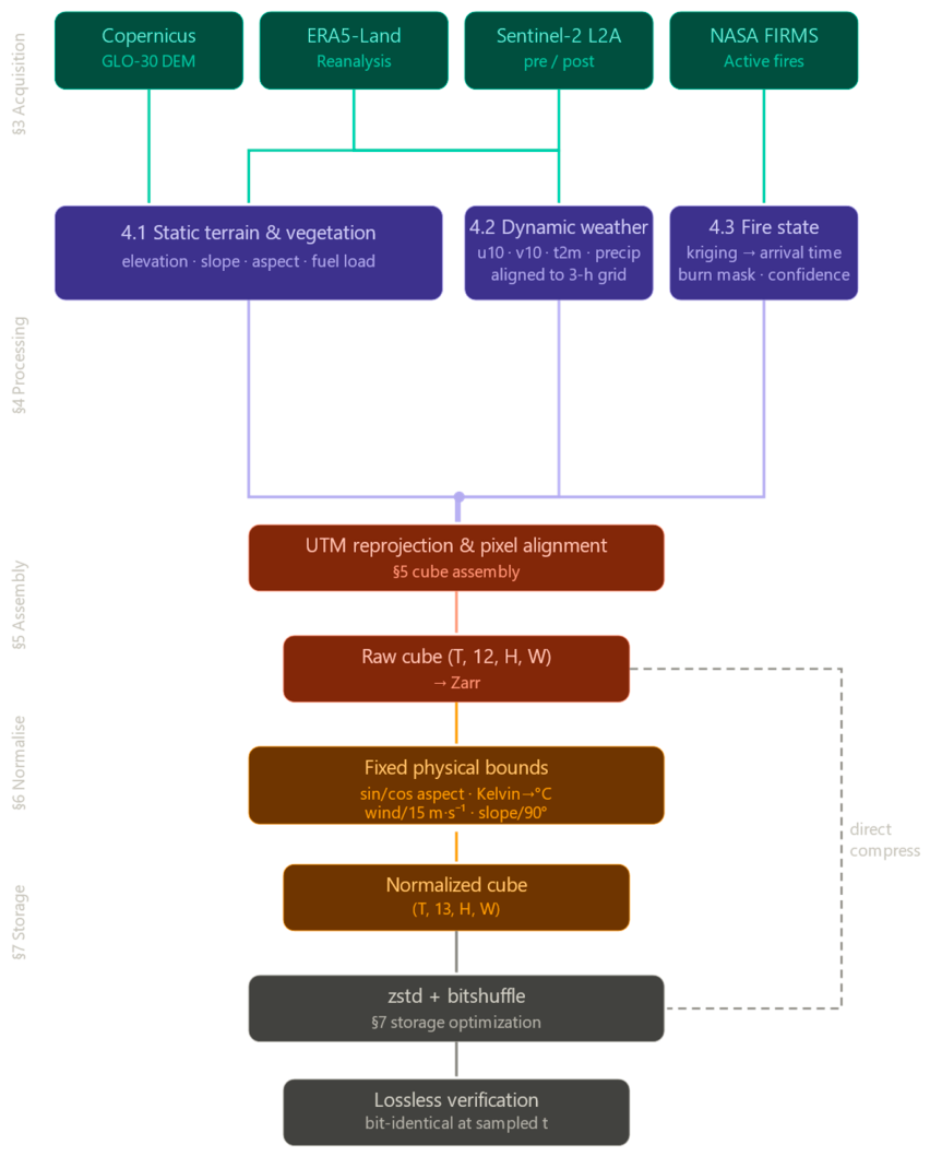
Figure 1 summarizes the end-to-end WildfireCube pipeline in a single flowchart, from raw data acquisition through processing, cube assembly, normalization, storage, and per-event quality assessment. Each block corresponds to a subsection in this paper; readers are encouraged to consult Figure 1 alongside the textual description below.

Figure 1. End-to-end WildfireCube pipeline flowchart. Acquisition stage (Section 3): Copernicus GLO-30 DEM, ERA5-Land reanalysis, Sentinel-2 L2A composites, and NASA FIRMS active-fire detections are independently fetched, cached, and isolated per event. Processing stage (Section 4): static terrain channels (elevation, slope, aspect, fuel load) are derived from the DEM and Sentinel-2 pre-fire imagery; dynamic weather channels are temporally aligned to the 3 h grid; fire state (arrival time, fire-front mask, fractional burn, observation confidence) is reconstructed via ordinary kriging of FIRMS detections. Cube assembly (Section 5): all channels are reprojected to an event-specific UTM zone, pixel-aligned, and persisted as a (T, 12, H, W) Zarr store. Normalization (Section 6): physics-informed transforms produce a (T, 13, H, W) ML-ready tensor. Storage optimization (Section 7): zstd + bitshuffle compression with lossless verification. Quality assessment (Section 9): per-event analytical reports report FIRMS density, kriging confidence, burn-severity reliability, weather-regime classification, and ML-readiness statistics. Constructing spatiotemporal wildfire progression cubes requires the fusion of heterogeneous geospatial datasets that differ in provider, spatial and temporal resolution, coordinate reference system, and delivery mechanism. The pipeline ingests four complementary datasets whose characteristics are summarized in Table 1. Together they supply the static terrain context, dynamic meteorological forcing, multispectral land-surface reflectance, and point-process active-fire observations needed to reconstruct fire spread at high resolution. All four are freely available under open-data licenses, ensuring full reproducibility. § = Section.

Figure 1. End-to-end WildfireCube pipeline flowchart. Acquisition stage (Section 3): Copernicus GLO-30 DEM, ERA5-Land reanalysis, Sentinel-2 L2A composites, and NASA FIRMS active-fire detections are independently fetched, cached, and isolated per event. Processing stage (Section 4): static terrain channels (elevation, slope, aspect, fuel load) are derived from the DEM and Sentinel-2 pre-fire imagery; dynamic weather channels are temporally aligned to the 3 h grid; fire state (arrival time, fire-front mask, fractional burn, observation confidence) is reconstructed via ordinary kriging of FIRMS detections. Cube assembly (Section 5): all channels are reprojected to an event-specific UTM zone, pixel-aligned, and persisted as a (T, 12, H, W) Zarr store. Normalization (Section 6): physics-informed transforms produce a (T, 13, H, W) ML-ready tensor. Storage optimization (Section 7): zstd + bitshuffle compression with lossless verification. Quality assessment (Section 9): per-event analytical reports report FIRMS density, kriging confidence, burn-severity reliability, weather-regime classification, and ML-readiness statistics. Constructing spatiotemporal wildfire progression cubes requires the fusion of heterogeneous geospatial datasets that differ in provider, spatial and temporal resolution, coordinate reference system, and delivery mechanism. The pipeline ingests four complementary datasets whose characteristics are summarized in Table 1. Together they supply the static terrain context, dynamic meteorological forcing, multispectral land-surface reflectance, and point-process active-fire observations needed to reconstruct fire spread at high resolution. All four are freely available under open-data licenses, ensuring full reproducibility. § = Section.

Table 1. Summary of data sources used in the WildfireCube pipeline.

Source	Provider	Native Resolution	Temporal Resolution	Key Variables
Copernicus GLO-30 DEM	ESA/Copernicus	30 m	Static	Elevation
ERA5-Land Reanalysis	ECMWF/Copernicus	~9 km (0.1 deg)	Hourly	10 m u/v wind, 2 m temperature, precipitation
Sentinel-2 L2A	ESA/Copernicus	10–60 m	5-day revisit	B04, B08, B11, B12
NASA FIRMS Active Fire	NASA	375 m (VIIRS)/1 km (MODIS)	Sub-daily	Hotspot lat/lon, Fire Radiative Power (FRP)

Table 1. Summary of data sources used in the WildfireCube pipeline.

Source	Provider	Native Resolution	Temporal Resolution	Key Variables
Copernicus GLO-30 DEM	ESA/Copernicus	30 m	Static	Elevation
ERA5-Land Reanalysis	ECMWF/Copernicus	~9 km (0.1 deg)	Hourly	10 m u/v wind, 2 m temperature, precipitation
Sentinel-2 L2A	ESA/Copernicus	10–60 m	5-day revisit	B04, B08, B11, B12
NASA FIRMS Active Fire	NASA	375 m (VIIRS)/1 km (MODIS)	Sub-daily	Hotspot lat/lon, Fire Radiative Power (FRP)

3.1. Copernicus GLO-30 Digital Elevation Model

Topography exerts first-order control on fire behavior: slope steepness accelerates uphill spread, aspect governs solar heating and fuel desiccation, and elevation correlates with vegetation type and moisture availability. The Copernicus GLO-30 Digital Elevation Model, Paris, France), derived from the TanDEM-X interferometric radar mission, provides global elevation at 30 m posting and serves as the static terrain layer. Elevation tiles are retrieved through the Copernicus Data Space Ecosystem (CDSE) SentinelHub processing API. Because SentinelHub imposes a hard limit of 2500 pixels per spatial dimension, large bounding boxes are decomposed into a regular tile grid and stitched after retrieval. Slope and aspect are derived via Horn’s finite-difference method on the stitched grid.

3.2. ERA5-Land Reanalysis

Weather conditions are the primary short-term driver of fire behavior. The ERA5-Land reanalysis product, produced by ECMWF (Reading, UK) within the Copernicus Climate Change Service, provides meteorological fields at approximately 9 km horizontal resolution and hourly temporal resolution. Four variables are requested per event via the Climate Data Store (CDS) API: 10 m eastward wind (u10), 10 m northward wind (v10), 2 m air temperature, and total precipitation. The CDS request area is padded by 0.5 degrees on every side of the fire bounding box to prevent boundary artifacts during subsequent bilinear interpolation. Coastal and island events may contain NaN values over ocean pixels; these are filled using nearest-neighbor extrapolation based on the Euclidean distance transform.

3.3. Sentinel-2 Level-2A Composites

Sentinel-2 provides multispectral imagery at 10–60 m resolution with a nominal five-day revisit interval. The Level-2A product, atmospherically corrected to bottom-of-atmosphere reflectance, is used to characterize pre-fire vegetation state and post-fire burn severity. Pre-fire and post-fire composites are constructed using the CDSE SentinelHub API with a 30-day temporal window and a LEAST_CC (least-cloud-cover) mosaicking strategy, which selects for each pixel the observation with the lowest cloud-cover percentage within the temporal window (Sentinel Hub Processing API documentation: https://docs.sentinel-hub.com/api/latest/data/sentinel-2-l2a/) (accessed on 20 March 2026), capped at a maximum 30% scene cloud cover. Four spectral bands are retrieved—B04 (Red, 665 nm), B08 (NIR, 842 nm), B11 (SWIR-1, 1610 nm), and B12 (SWIR-2, 2190 nm)—supporting computation of the normalized burn ratio and its variants.

3.4. NASA FIRMS Active-Fire Detections

The temporal dimension of fire progression is captured by active-fire hotspot detections from the NASA Fire Information for Resource Management System (FIRMS; NASA, Greenbelt, MD, USA), which aggregates thermal anomaly detections from VIIRS (375 m resolution) and MODIS (1 km resolution). Because the FIRMS REST API imposes a maximum window of five days per request, the full event duration is partitioned into consecutive five-day chunks. Four sources are queried: VIIRS_NOAA20_SP, VIIRS_SNPP_SP, MODIS_SP, and VIIRS_NOAA21_NRT. Detections are concatenated and a combined acquisition timestamp is parsed from the acq_date and acq_time fields. Events with fewer than six total hotspot detections are flagged, as sparse observations may compromise the reliability of kriging-based spatial interpolation.

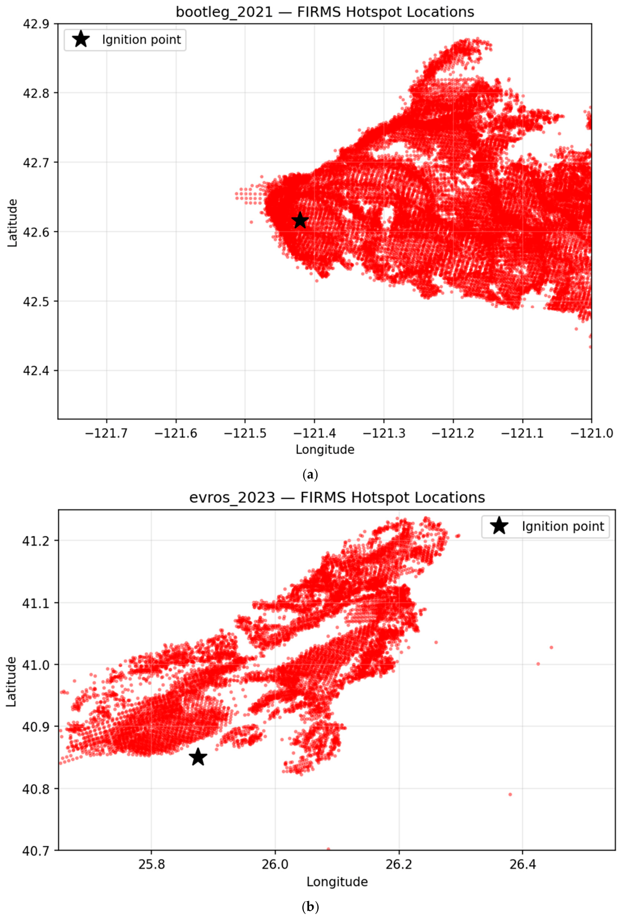
Figure 2 illustrates the spatial distribution of FIRMS active-fire detections for two representative events from distinct fire regimes. Each point corresponds to a single VIIRS or MODIS thermal anomaly detection, plotted in geographic coordinates with the estimated ignition point marked. The Bootleg 2021 fire (Oregon, USA) produced 22,983 detections across a montane landscape over 15 days, with the scatter revealing a complex, branching fire perimeter shaped by ridgelines and valley corridors. In contrast, the Evros 2023 fire (Greece) yielded 10,109 detections over 15 days in a comparatively flat terrain, producing a more compact cluster driven by sustained Etesian winds. The density and spatial pattern of these detections directly govern the quality of the kriging-interpolated arrival-time surface described in Section 4.3.1: denser clusters yield tighter confidence intervals, while sparse peripheral detections increase interpolation uncertainty. Comparing events across fire regimes reveals that detection density does not scale linearly with burned area; it depends on satellite overpass frequency, cloud cover during the event, and the fire’s temporal overlap with overpass schedules. These factors motivate the observation confidence channel (Section 4.3.4), which provides a per-pixel quality indicator derived from local detection density.

3.5. Acquisition Robustness

A multi-event processing pipeline must tolerate transient failures across independent web services. Rate-limit awareness (five-day FIRMS chunks, CDS long-running jobs), disk caching with a skip-fetch flag, and per-event isolation ensure that the acquisition pipeline can process large event catalogs with minimal manual intervention. If a data source fails for one event, processing continues with the remaining events and interrupted batch runs can be safely resumed.

Pipeline performance across the 13 demonstration events is summarized quantitatively as follows. End-to-end processing succeeded for 13/13 events (100% success rate); lossless Zarr re-compression passed bit-identical verification at all sampled timesteps for 13/13 events (Section 7.2); and per-pixel grid alignment between the four source datasets was exact by construction after UTM reprojection (Section 5.2). Pipeline behavior was further evaluated across three distinct fire-acquisition regimes: (i) dense-detection events (Creek 2020, 39,791 FIRMS detections), where kriging confidence was high across the burned domain; (ii) moderate-detection events (median ~10,891 detections, e.g., Evros, Bootleg), where kriging confidence remained reliable across the fire-front region; and (iii) sparse-detection events (Eagle Creek 2017, 948 detections), where the pipeline still produced a valid tensor but the observation-confidence channel (Section 4.3.4) correctly down-weights interpolated regions for downstream ML loss masking. Across all events, the FIRMS-density-derived observation-confidence channel was non-degenerate (mean per-event > 0.3), the kriging arrival-time surface was successfully reconstructed (zero failed events), and the static and dynamic channels were complete with no missing temporal bins. These quantitative results, together with the per-event analytical reports in Section 9 demonstrate that pipeline performance is robust across diverse fire regimes, terrain types, and observational densities.

4. Data Processing Pipeline

This section describes the data-processing stage of the pipeline shown in Figure 1. The pipeline derives static terrain and vegetation layers from the GLO-30 DEM and Sentinel-2 imagery (Section 4.1), aligns dynamic ERA5-Land weather variables to the 3 h temporal grid (Section 4.2), and reconstructs the evolving fire state from FIRMS active-fire detections (Section 4.3).

4.1. Static Terrain and Vegetation Layers

The pipeline derives four static channels from the GLO-30 DEM and Sentinel-2 composites (Table 2). These channels are time-invariant and broadcast identically across all T temporal slices.

4.1.1. Slope and Aspect via Horn’s Method

Slope is computed from the DEM using the central finite-difference approximation (Horn’s method) on a 3 × 3 pixel neighborhood. The partial derivatives of elevation z with respect to x (east) and y (north) are estimated as

dz/dx = (z_i,j+1 − z_i,j−1)/(2Δ)

(2)

dz/dy = (z_i−1,j − z_i+1,j)/(2Δ)

(3)

where Δ is the pixel spacing in meters (30 m). Forward and backward differences are substituted at grid boundaries. Slope in degrees follows as

S = arctan(√((∂z/∂x)² + (∂z/∂y)²))

(4)

and aspect is obtained from

A = atan2(−∂z/∂x, ∂z/∂y)

(5)

mapped to [0 degrees, 360 degrees) with north as reference.

4.1.2. Spectral Vegetation and Burn-Severity Indices

Five spectral indices are computed from Sentinel-2 L2A surface reflectance. The normalized burn ratio (NBR) contrasts NIR (B08) and SWIR-2 (B12): NBR = (rho_NIR − rho_SWIR2)/(rho_NIR + rho_SWIR2), where rho denotes bottom-of-atmosphere surface reflectance. Burn severity is quantified by the Relativized Burn Ratio (RBR), which normalizes the temporal NBR change by pre-fire vegetation state:

RBR = dNBR/(NBR_pre + 1.001)

(6)

where dNBR = NBR_pre − NBR_post. The additive offset of 1.001 follows the original RBR formulation of Parks et al. [20]. The value 1.001 (rather than 1.0) guarantees a strictly positive denominator across the full physical NBR range [−1, 1]: an exact pre-fire NBR of −1, which can occur over fully non-vegetated surfaces such as bare rock or water, would otherwise drive NBR_pre + 1.0 to zero. The 0.001 increment removes this singularity while introducing negligible bias in vegetated pixels (relative perturbation <0.1% for NBR_pre > 0). RBR correlates more strongly with field-assessed burn severity than dNBR alone, particularly in ecosystems with heterogeneous pre-fire canopy cover, and is adopted as the primary severity metric. The Normalized Difference Vegetation Index (NDVI = (NIR − Red)/(NIR + Red)) and Normalized Difference Moisture Index (NDMI = (NIR − SWIR1)/(NIR + SWIR1)) are also computed from pre-fire imagery.

4.1.3. Fuel Load Index

A composite Fuel Load Index F_l fuses vegetation abundance, moisture status, burn propensity, and terrain slope into a single scalar field:

F_l = (NDVI × NBR_pre)/(1 − NDMI) × (1 + tan(φ))

(7)

where φ is the local slope angle in radians. NDVI quantifies photosynthetically active biomass; NBR_pre adds canopy-structure context; the 1/(1 − NDMI) term in the formula acts as an inverse moisture limitation (drier fuel yields higher F_l); and the slope factor 1 + tan(φ) reflects the well-established relationship whereby steeper terrain accelerates fire spread through enhanced radiative preheating. F_l is a relative predisposition index, not a direct measurement of fuel biomass in physical units.

Table 2. Static channels in the spatiotemporal data cube.

Channel	Source	Units	Physical Role
Elevation	GLO-30 DEM	meters	Altitude; proxy for temperature lapse and vegetation type
Slope	Horn’s method on DEM	degrees	Gradient steepness; governs convective preheating and rate of spread
Aspect	Horn’s method on DEM	degrees (CW from N)	Direction of steepest descent; solar exposure and dominant spread axis
Fuel Load	NDVI, NBR, NDMI, slope	dimensionless	Relative burn predisposition; fuses vegetation condition with terrain

Table 2. Static channels in the spatiotemporal data cube.

Channel	Source	Units	Physical Role
Elevation	GLO-30 DEM	meters	Altitude; proxy for temperature lapse and vegetation type
Slope	Horn’s method on DEM	degrees	Gradient steepness; governs convective preheating and rate of spread
Aspect	Horn’s method on DEM	degrees (CW from N)	Direction of steepest descent; solar exposure and dominant spread axis
Fuel Load	NDVI, NBR, NDMI, slope	dimensionless	Relative burn predisposition; fuses vegetation condition with terrain

4.2. Dynamic Weather Layers

The meteorological layer draws on ERA5-Land at approximately 9 km native resolution. Bilinear interpolation via xarray.DataArray.interp() is applied to downscale weather fields to the target grid. The interpolation domain is expanded by 0.5 degrees on every side to prevent edge artifacts. For large domains, the effective resolution is capped at 1 km before the reprojection stage performs the final upsampling to 30 m; interpolating below 1 km yields no additional information content from a 9 km source. Interpolation is executed in temporal chunks of 24 timesteps to bound peak memory usage.

Wind fields are stored as orthogonal Cartesian components u10 (eastward) and v10 (northward) rather than scalar speed and direction. This representation avoids the circular discontinuity at 0 degrees/360 degrees and preserves the sign convention necessary for computing directional projections (e.g., along-slope wind component). Scalar wind speed s = sqrt(u² + v²) and meteorological direction theta = atan2(u, v) are recoverable analytically. ERA5-Land provides four variables per event: u10, v10, 2 m temperature (in Kelvin), and total precipitation (in meters of water equivalent per hour).

ERA5-Land is a land-only product, so coastal and island domains contain missing data (NaN) values over ocean pixels. These are filled using nearest-neighbor extrapolation based on the Euclidean distance transform: for each NaN pixel, scipy.ndimage.distance_transform_edt identifies the closest valid land pixel, and the NaN is replaced by that value. For events in this study, the affected fraction ranges from under 1% (Evros) to approximately 8% (Lahaina, where the domain extends over open ocean).

ERA5-Land hourly fields are assigned to 3 h temporal bins by retaining the hourly sample closest to each bin midpoint. The 3 h default captures essential diurnal variation (morning upslope winds, afternoon peak temperatures, nocturnal inversions) while reducing the temporal dimension of the cube by a factor of three relative to hourly storage. The bin width is user-configurable without modifying the fetching logic.

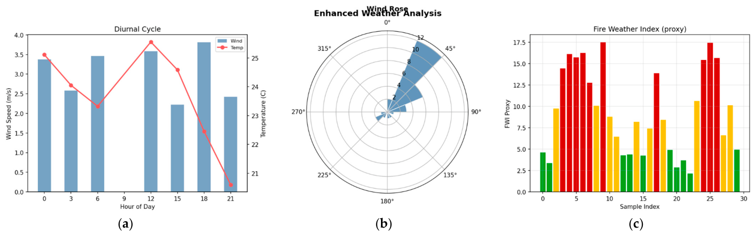
Figure 3 presents the enhanced weather analysis for a representative event, decomposing the ERA5-Land meteorological channels into three complementary views. Panel (a) shows the diurnal cycle of wind speed (bars, left axis) and 2 m air temperature (line, right axis), averaged across the full event domain and aggregated into the 3 h temporal bins used by the cube. The characteristic diurnal pattern is evident: wind speeds peak during late afternoon and nighttime hours (reaching 3.0–3.5 m/s) when thermal gradients drive slope and valley winds, while temperature follows the expected solar cycle with a midday maximum near 30 degrees C and a pre-dawn minimum near 14 degrees C. This diurnal coupling between wind and temperature is a primary driver of fire behavior: maximum spread rates typically coincide with the late-afternoon combination of elevated temperature, low humidity, and strong winds.

Panel (b) displays a wind rose computed from the u10 and v10 ERA5-Land wind components across all timesteps, revealing the dominant wind direction and speed distribution. This visualization explains the directional bias observed in fire spread patterns; fires in this event propagated primarily downwind along the dominant axis visible in the wind rose. Panel (c) shows the Fire Weather Index (FWI) proxy, a composite metric derived from temperature and wind speed that serves as an indicator of fire weather severity. The color coding (green = low, yellow = moderate, orange = high, dark red = extreme) identifies periods of critical fire weather. Peaks in the FWI proxy correspond to episodes of rapid fire spread visible in the arrival-time surface (Figure 4), confirming the tight coupling between meteorological forcing and fire behavior captured by the dynamic channels of the WildfireCube tensor.

4.3. Fire-State Reconstruction

Fire state is reconstructed from NASA FIRMS hotspot detections through a five-stage pipeline producing four channels per temporal bin: fire-front mask, RBR severity, fractional burn, and observation confidence.

4.3.1. Fire Arrival Time via Ordinary Kriging

The fundamental challenge is to convert an irregular scatter of hotspot detections into a continuous field describing when the fire reached each location. For each hotspot i with acquisition timestamp t_i, the elapsed time relative to the temporal origin t_origin = min_i(t_i) is computed as h_i = (t_i − t_origin)/3600 (in hours). The interpolation domain is discretized onto a 30 m grid. Ordinary kriging with a spherical variogram model is used as the preferred interpolation method when: (i) the hotspot count lies in [6, 200], and (ii) the output grid contains no more than 250,000 pixels. Kriging exploits the spatial autocorrelation structure of fire arrival times and provides a best linear unbiased prediction. When kriging is infeasible, the pipeline falls back to Delaunay-based linear interpolation via scipy.griddata.

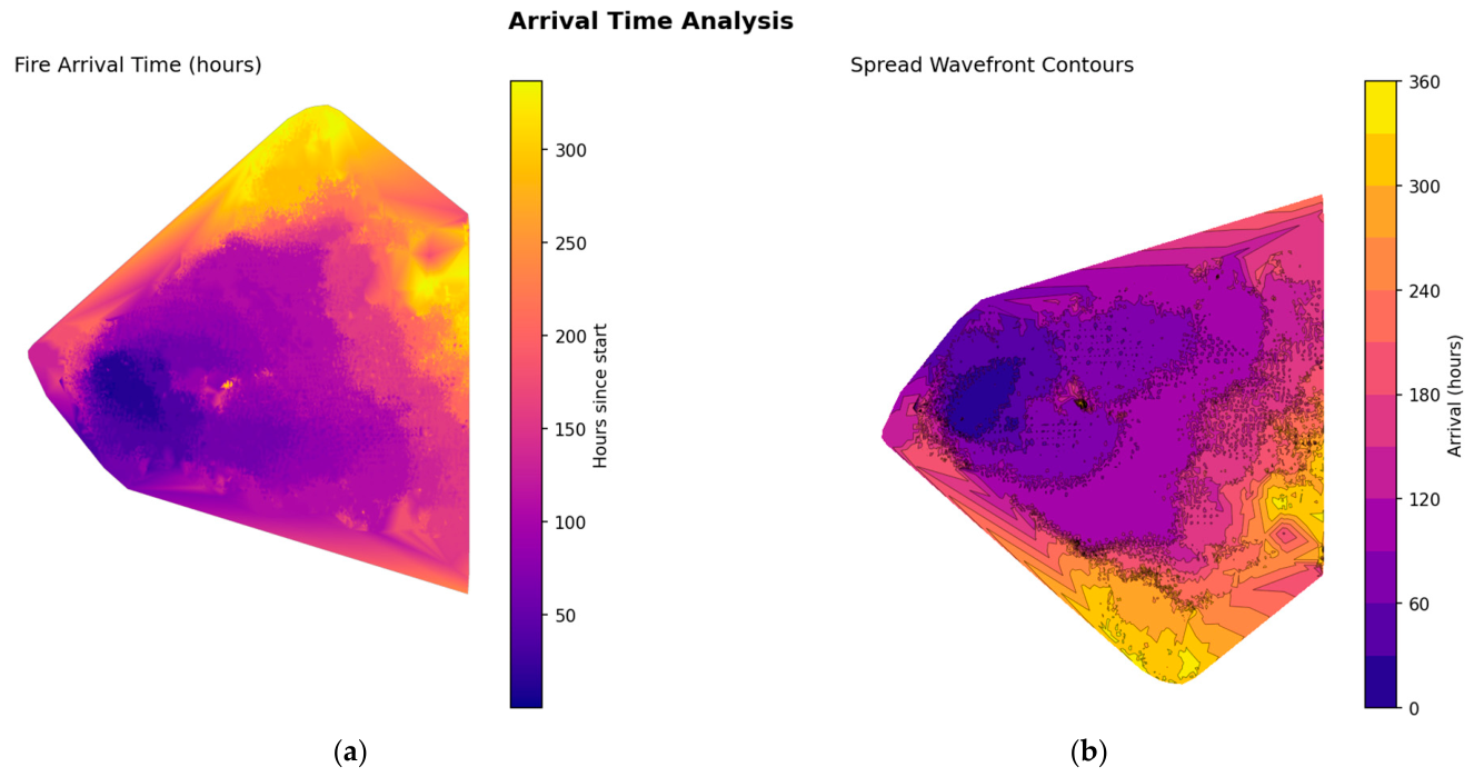
Figure 4 demonstrates the core output of the fire-state reconstruction pipeline for a representative event. Panel (a) shows the continuous fire arrival-time surface produced by ordinary kriging, expressed as hours since the first FIRMS detection. The color gradient from dark (early arrival, near the ignition point) to bright (late arrival, at the fire perimeter) reveals the spatial progression of the fire over its full duration. Regions of gradual color transitions indicate steady, low-velocity spread through continuous fuels, while abrupt color boundaries mark terrain barriers (ridgelines, water bodies, roads) or sudden wind shifts that temporarily halted or redirected the fire front. The smooth interpolation produced by kriging contrasts with the discrete, irregular scatter of FIRMS detections shown in Figure 2, illustrating the value of geostatistical interpolation for converting sparse satellite observations into the dense, grid-regular fields required by convolutional architectures.

Panel (b) presents the same arrival-time surface as contour lines at regular intervals (e.g., every 24 h), producing a wavefront map that directly visualizes the fire’s propagation history. Closely spaced contours indicate rapid spread during wind-driven episodes, while widely spaced contours correspond to periods of slow, creeping spread or temporary suppression. The wavefront representation is particularly informative for identifying episodic extreme behavior: for instance, a cluster of contour lines compressed into a narrow band reveals a wind-driven run event where the fire advanced several kilometers in a single 3 h timestep. These arrival-time surfaces are subsequently thresholded into the binary fire-front masks and fractional burn channels described below, ensuring that each temporal slice of the tensor encodes a physically consistent snapshot of the fire’s spatial extent at that moment.

4.3.2. Binary Fire-Front Mask

The arrival-time surface is thresholded into discrete temporal bins. For a bin [t0, t1), a pixel is classified as actively burning if its estimated arrival time A(x,y) satisfies t0 ≤ A(x,y) < t1. The resulting binary mask (uint8) provides a crisp burned/unburned classification suitable for direct use as a binary classification target.

4.3.3. Fractional Burn

To mitigate temporal aliasing in binary thresholding, a fractional burn channel encodes the proportion of each bin during which a pixel has been in a burned state:

frac(x,y) = 0 if A ≥ t₁ or NaN
frac(x,y) = 1 if A < t₀
frac(x,y) = (t₁ − A)/(t₁ − t₀) if t₀ ≤ A < t₁

(8)

This piecewise-linear formulation provides smoother gradients during training and preserves sub-bin temporal information. A pixel burning at the bin’s onset receives frac = 1; one burning at the bin’s close receives frac ~= 0; intermediate arrivals are linearly interpolated.

4.3.4. Observation Confidence

Not all regions of the arrival-time surface are equally trustworthy. Pixels near observed hotspots are well-constrained, while those far from any detection rely entirely on the interpolator’s assumptions. For each temporal bin, an observation confidence channel is computed as

conf(x,y) = min(1, count/10)

(9)

where count is the number of FIRMS detections falling within the bin at each grid cell. Bins with 10 or more hotspots receive the maximum confidence of 1.0; bins with zero detections (purely interpolated) receive 0.0. This channel can be used to weight the training loss, assigning a lower penalty to predictions in poorly observed regions.

5. Cube Assembly Architecture

5.1. Channel Layout

The assembled cube contains C = 12 channels organized into three semantic blocks. After physics-informed normalization (Section 6), the cube contains C = 13 channels: the circular aspect channel is decomposed into a (sin, cos) pair, increasing the channel count by one. Throughout this paper, we therefore refer to two tensor variants—the raw (T, 12, H, W) cube and the normalized (T, 13, H, W) ML-ready cube—and the channel count cited at any point reflects which variant is being discussed.

Table 3. Complete channel layout of the raw (T, 12, H, W) WildfireCube.

Index	Category	Channel	Source	Units
0	Static	Elevation	GLO-30 DEM	meters
1	Static	Slope	DEM (Horn)	degrees
2	Static	Aspect	DEM (Horn)	degrees [0, 360)
3	Static	Fuel Load	Sentinel-2 pre-fire	dimensionless
4	Dynamic	U-wind 10 m	ERA5-Land	m/s
5	Dynamic	V-wind 10 m	ERA5-Land	m/s
6	Dynamic	Temperature 2 m	ERA5-Land	Kelvin
7	Dynamic	Precipitation	ERA5-Land	meters
8	State	Fire-front mask	FIRMS kriging	binary {0, 1}
9	State	RBR severity	Sentinel-2 pre/post	dimensionless
10	State	Fractional burn	FIRMS kriging	[0, 1]
11	State	Observation confidence	FIRMS density	[0, 1]

details the complete channel layout. Static channels occupy the lowest indices; dynamic weather channels follow; and the final block encodes the evolving fire state. The RBR severity channel is placed in the state block because it semantically describes fire impact, even though it is derived from a single pre-/post-fire image pair and broadcast across all T timesteps.

5.2. UTM Reprojection and Grid Alignment

Source layers arrive in geographic coordinates (EPSG:4326). Because metric distances are essential for physically meaningful convolution kernels, every layer is reprojected onto an event-specific Universal Transverse Mercator (UTM) zone before assembly. The UTM zone is determined from the centroid longitude of the event bounding box, choosing the zone that minimizes metric distortion within the fire’s spatial extent. Reprojection is performed with rasterio.warp.reproject using bilinear resampling. All twelve channels share an identical pixel grid by using the same destination transform, CRS, and grid shape, so arrays are pixel-aligned by construction. A nearest-neighbor fill based on the Euclidean distance transform removes thin wedges of NaN pixels at raster borders introduced by the UTM rotation.

5.3. Zarr Storage and Tiling

The assembled cube is persisted as a Zarr store with chunk shape (1, 12, 256, 256): one temporal slice at full channel depth spanning a 256 × 256 spatial tile (~7.68 km × 7.68 km at 30 m). This layout enables efficient random access during training without loading the entire cube into memory. Event-level metadata (channel names, CRS, bounding box, date range, resolution) are written into the store’s .zattrs dictionary, so downstream consumers can discover the cube structure programmatically.

The cube is further subdivided into overlapping 256 × 256 patches for training. Patches are extracted with a stride of 224 pixels (32-pixel overlap). The overlap provides border context for edge predictions and enables seamless spatial stitching during inference. Boundary patches are zero-padded with NaN to preserve uniform tensor shape. Each patch retains full temporal and channel depth, yielding arrays of shape (T, 12, 256, 256).

6. Physics-Informed Normalization Framework

6.1. Motivation

Standard normalization strategies (min-max rescaling, z-score standardization) treat every channel as an interchangeable numeric array, computing sample-level statistics and linearly mapping values into a convenient interval. Three classes of structure are lost when this is applied blindly to the WildfireCube: (i) bounded variables such as slope are physically constrained to [0, 90 degrees] but z-scoring allows tails beyond this range; (ii) circular variables such as aspect define 0 degrees and 360 degrees as identical but any linear mapping maximizes their Euclidean distance; and (iii) signed vector components such as wind must share a common scale to preserve directional information.

The physics-informed framework instead derives each transform from the mathematical nature and operational range of the variable. Divisors correspond to physical maxima or climatological reference values; circular variables are projected onto a trigonometric basis; and already-bounded channels pass through unchanged. Because transform parameters are fixed physical constants rather than data-derived statistics, the normalization is identical across events, enabling direct cross-event comparison and transfer, and is exactly invertible up to clipping at distributional tails.

6.2. Transform Table

The normalization stage ingests a raw cube of shape (T, 12, H, W) and produces a normalized cube of shape (T, 13, H, W). The additional channel arises from the sinusoidal encoding of aspect, which splits one circular channel into sine and cosine components.

Table 4. Physics-informed normalization transforms. Aspect is split into two channels (sine and cosine), yielding 13 channels from 12 raw channels.

Raw Channel	Method	Formula	Output Range
Elevation (m)	divide	x/1000	~[0, 3]
Slope (deg)	divide	x/90	[0, 1]
Aspect (deg)	sincos	sin(x ∗ pi/180), cos(x ∗ pi/180)	[−1, 1]
Fuel Load	passthrough	x	raw
U-wind (m/s)	divide	x/15	~[−1, 1]
V-wind (m/s)	divide	x/15	~[−1, 1]
Temperature (K)	kelvin_to_norm	(K-273.15→C), clip [−5, 45], (C + 5)/50	[0, 1]
Precipitation (m)	m_to_mm_norm	x ∗ 1000, clip [0, 10], /10	[0, 1]
Fire-front mask	passthrough	x	{0, 1}
RBR	clip	clip [−0.5, 1.0]	[−0.5, 1.0]
Fractional burn	passthrough	x	[0, 1]
Obs. confidence	passthrough	x	[0, 1]

details the complete transform mapping.

6.3. Transform Rationale

Elevation divided by 1000 converts meters to kilometers, yielding ~[0, 3] for the events in the catalog. The divisor is a unit conversion factor, so the normalized value retains direct physical meaning through the dry adiabatic lapse rate (~6.5 °C/km). Slope is divided by its physical maximum of 90 degrees, mapping the channel to [0, 1] with the interpretation that 0.5 corresponds to a 45-degree incline. Aspect is decomposed into sine and cosine components, placing nearby directions close in Euclidean space regardless of the 0/360-degree branch cut, while preserving full directional information (theta = atan2(sin, cos)). Wind components u10 and v10 are divided by 15 m/s, the 99th-percentile fire-weather threshold in the catalog; both components share the same divisor so the implied wind direction is undistorted. Temperature undergoes a three-step transform: Kelvin to Celsius, clip to [−5, 45] °C (the operational fire-weather range), then affine rescale to [0, 1] via (C + 5)/50. Precipitation is converted from meters to millimeters, clipped at 10 mm (the heavy-rainfall threshold above which fire activity is uniformly suppressed), and divided by 10. RBR is clipped to [−0.5, 1.0] to remove pathological values arising from near-zero pre-fire NBR denominators. The four remaining channels (fuel load, fire-front mask, fractional burn, observation confidence) pass through unchanged as they are already bounded by construction.

7. Storage Optimization and Compression

A single event at 30 m resolution over several weeks can exceed 8 GB in its raw float32 representation. Efficient storage is therefore a prerequisite for working with a multi-event catalog at scale. Zarr organizes an N-dimensional array into a regular grid of fixed-size chunks, each compressed independently as a separate file. This architecture supports lazy loading, concurrent reads from multiple processes (unlike HDF5 in default mode), and direct compatibility with cloud object stores.

7.1. Default and Optimized Compression

During cube assembly, Zarr arrays are written with the Blosc meta-compressor configured with the LZ4 codec, optimized for decompression throughput (>3 GB/s). After analysis and report generation are complete, each cube is recompressed with Zstandard (zstd) at compression level 5 with the bitshuffle pre-filter. Bitshuffle transposes the bits of consecutive float32 values into 32 independent bit-planes, producing long runs of identical bits in the sign and exponent bytes that compress efficiently under entropy coding. The combined effect on a representative event (cedar_creek_2022, shape (112, 12, 1344, 1141), dtype float32) is shown in

Table 5. Compression results for the cedar_creek_2022 event cube.

Metric	Value
Logical size (float32)	8.24 GB
Stored size (LZ4 default)	4.44 GB (1.86× ratio)
Stored size (zstd level 5 + bitshuffle)	3.20 GB (2.58× ratio)
Additional savings over LZ4	1.24 GB (28% reduction)
Compression wall time	~55 s

.

7.2. Lossless Verification

Recompression must be strictly lossless. After writing the compressed copy to a temporary path, three timesteps (t = 0, T/2, T − 1) are read from both the original and compressed stores. Two assertions are evaluated per timestep: (i) numpy.array_equal confirms all finite values are bit-identical; (ii) numpy.array_equal on isnan() confirms the spatial NaN pattern is preserved, guarding against codec edge cases. Only after all assertions pass does the pipeline atomically replace the original store. All events in the current catalog passed verification at every sampled timestep. Across the 13-event initial catalog, deletion of patches and intermediate files reclaimed ~250 GB; combined with zstd recompression, total disk footprint was reduced by over 60%.

8. Event Catalog

Event Selection Rationale

The target catalog comprises wildfire events spanning the period of 2016–2024 across the United States, Canada, and Greece, deliberately constructed to sample a broad range of fire regimes. Events were selected to (i) have sufficient FIRMS hotspot detections for reliable arrival-time kriging; (ii) fall within the temporal coverage of all four data sources; and (iii) span a range of burned areas from moderate to large. From a broader pool of candidate events, 13 have been fully processed through the pipeline and are presented in this paper as demonstration runs. Table 6 presents these 13 processed events with key descriptive statistics. Note on RBR outliers: RBR mean values marked with an asterisk (*) in Table 6 are negative or unphysically large in magnitude because, over pixels with sparse pre-fire vegetation, NBR_pre approaches its lower bound of −1 and the RBR denominator (NBR_pre + 1.001) becomes near-zero, amplifying numerator noise. Per-pixel RBR remains physically meaningful over vegetated burned areas within those events; the spatial-mean statistic is the quantity that is contaminated. For ML training and downstream analysis we handle these outliers as follows: (i) RBR is clipped to the physical range [−0.5, 1.0] during normalization (Section 6.2, Table 4); (ii) for the eight events with negative spatial-mean RBR we recommend using the per-pixel dNBR channel as a more robust severity signal (Section 9.4); and (iii) the high-severity-fraction metric reported in Table 7 and Section 9.4 is restricted to pixels with reliable RBR, so the catalog-wide severity statistics are not biased by these outliers.

9. Extended Cross-Event Analysis and ML Readiness

This section provides a comprehensive cross-event comparison drawing on the full suite of analytical metrics extracted from per-event reports. Table 7 presents extended statistics covering Fire Radiative Power (FRP), maximum wind speed, Fire Weather Index (FWI) proxy, peak spread rate, and high-severity fraction, complementing the descriptive statistics of Table 6. Table 8 summarizes aggregate statistics across the 13-event processed catalog, and Table 9 provides the catalog-wide dataset scale summary.

Table 6. Complete event catalog with descriptive statistics. * denotes events with pathological RBR values due to sparse pre-fire vegetation.

#	Event	Country	Year	Duration (Days)	Burned (km2)	Burned Frac (%)	RBR Mean	Wind (m/s)	Temp (°C)
1	Bootleg	USA	2021	15	24.56	0.62	0.130	2.17	23.76
2	Calf Canyon/Hermits Peak	USA	2022	14	42.73	0.45	0.072	2.87	8.83
3	Cameron Peak	USA	2020	14	13.34	0.32	0.030	1.43	19.78
4	Carr	USA	2018	14	22.61	1.01	−24.64 *	1.14	25.74
5	Cedar Creek	USA	2022	14	22.05	1.64	0.052	1.39	18.48
6	Chuckegg Creek	Canada	2019	14	31.05	0.42	−0.177	2.25	13.28
7	Creek	USA	2020	13	89.10	2.59	−6.29 *	1.40	19.71
8	Dixie	USA	2021	14	93.26	1.10	−2.20 *	1.58	24.85
9	Eagle Creek	USA	2017	11	59.32	2.98	−7.71 *	1.42	22.89
10	East Troublesome	USA	2020	12	86.39	2.09	−1.11	2.66	2.47
11	Elephant Hill	Canada	2017	15	20.50	0.43	−1.25	1.70	19.08
12	Evia	Greece	2021	10	165.69	8.63	0.078	2.33	29.18
13	Evros	Greece	2023	15	188.44	4.09	−0.338	3.88	25.79

Burned (km²): total area classified as burned by the cumulative fire-front mask. Burned Frac (%): burned area as a percentage of total bounding-box area. RBR mean: spatial average over burned pixels. Wind (m/s) and Temp (°C): spatiotemporal averages over the full cube domain and duration.

Table 6. Complete event catalog with descriptive statistics. * denotes events with pathological RBR values due to sparse pre-fire vegetation.

#	Event	Country	Year	Duration (Days)	Burned (km2)	Burned Frac (%)	RBR Mean	Wind (m/s)	Temp (°C)
1	Bootleg	USA	2021	15	24.56	0.62	0.130	2.17	23.76
2	Calf Canyon/Hermits Peak	USA	2022	14	42.73	0.45	0.072	2.87	8.83
3	Cameron Peak	USA	2020	14	13.34	0.32	0.030	1.43	19.78
4	Carr	USA	2018	14	22.61	1.01	−24.64 *	1.14	25.74
5	Cedar Creek	USA	2022	14	22.05	1.64	0.052	1.39	18.48
6	Chuckegg Creek	Canada	2019	14	31.05	0.42	−0.177	2.25	13.28
7	Creek	USA	2020	13	89.10	2.59	−6.29 *	1.40	19.71
8	Dixie	USA	2021	14	93.26	1.10	−2.20 *	1.58	24.85
9	Eagle Creek	USA	2017	11	59.32	2.98	−7.71 *	1.42	22.89
10	East Troublesome	USA	2020	12	86.39	2.09	−1.11	2.66	2.47
11	Elephant Hill	Canada	2017	15	20.50	0.43	−1.25	1.70	19.08
12	Evia	Greece	2021	10	165.69	8.63	0.078	2.33	29.18
13	Evros	Greece	2023	15	188.44	4.09	−0.338	3.88	25.79

Burned (km²): total area classified as burned by the cumulative fire-front mask. Burned Frac (%): burned area as a percentage of total bounding-box area. RBR mean: spatial average over burned pixels. Wind (m/s) and Temp (°C): spatiotemporal averages over the full cube domain and duration.

Table 7. Extended per-event metrics from event report analytics. FRP = Fire Radiative Power. FWI = Fire Weather Index proxy (temperature–wind composite). Max spread = peak 3 h spread rate in km² per timestep. High sev = fraction of burned pixels exceeding the high-severity RBR threshold (>0.27).

Event	FIRMS Det.	FRP Mean (MW)	FRP Max (MW)	Max Wind (m/s)	FWI Mean	FWI Max	Max Spread (km2/3 h)	High Sev (%)
Bootleg 2021	22,983	57.7	5617	4.53	20.0	51.6	7.65	28.3
Calf Cyn/HP 2022	10,891	57.3	8996	11.02	14.5	75.5	40.51	10.6
Cameron Peak 2020	3908	46.4	4111	4.83	7.7	27.3	2.80	4.8
Carr 2018	15,579	33.6	2287	4.08	6.8	22.6	8.11	23.7
Cedar Creek 2022	11,358	48.8	9321	3.39	8.7	39.0	8.61	23.4
Chuckegg Creek 2019	12,617	54.1	7970	4.88	8.1	28.2	15.05	3.8
Creek 2020	39,791	36.9	6206	3.66	11.2	47.2	66.48	20.4
Dixie 2021	24,626	49.0	9732	3.99	15.0	50.7	37.08	0.1
Eagle Creek 2017	948	40.2	1615	3.42	9.4	39.3	55.99	1.0
East Troublesome 2020	10,410	78.1	16,146	7.17	7.5	42.2	37.34	3.4
Elephant Hill 2017	7318	68.3	3291	3.51	6.4	30.2	11.40	31.5
Evia 2021	7730	43.0	5285	5.72	9.8	29.8	150.75	31.1
Evros 2023	10,109	45.2	4612	9.10	9.4	17.5	116.69	19.2

Eagle Creek 2017 has a markedly low FIRMS detection count (948) due to sparse overpass coverage during this event; the kriging-based arrival surface for this event relies on fewer ground points and carries wider uncertainty.

Table 7. Extended per-event metrics from event report analytics. FRP = Fire Radiative Power. FWI = Fire Weather Index proxy (temperature–wind composite). Max spread = peak 3 h spread rate in km² per timestep. High sev = fraction of burned pixels exceeding the high-severity RBR threshold (>0.27).

Event	FIRMS Det.	FRP Mean (MW)	FRP Max (MW)	Max Wind (m/s)	FWI Mean	FWI Max	Max Spread (km2/3 h)	High Sev (%)
Bootleg 2021	22,983	57.7	5617	4.53	20.0	51.6	7.65	28.3
Calf Cyn/HP 2022	10,891	57.3	8996	11.02	14.5	75.5	40.51	10.6
Cameron Peak 2020	3908	46.4	4111	4.83	7.7	27.3	2.80	4.8
Carr 2018	15,579	33.6	2287	4.08	6.8	22.6	8.11	23.7
Cedar Creek 2022	11,358	48.8	9321	3.39	8.7	39.0	8.61	23.4
Chuckegg Creek 2019	12,617	54.1	7970	4.88	8.1	28.2	15.05	3.8
Creek 2020	39,791	36.9	6206	3.66	11.2	47.2	66.48	20.4
Dixie 2021	24,626	49.0	9732	3.99	15.0	50.7	37.08	0.1
Eagle Creek 2017	948	40.2	1615	3.42	9.4	39.3	55.99	1.0
East Troublesome 2020	10,410	78.1	16,146	7.17	7.5	42.2	37.34	3.4
Elephant Hill 2017	7318	68.3	3291	3.51	6.4	30.2	11.40	31.5
Evia 2021	7730	43.0	5285	5.72	9.8	29.8	150.75	31.1
Evros 2023	10,109	45.2	4612	9.10	9.4	17.5	116.69	19.2

Eagle Creek 2017 has a markedly low FIRMS detection count (948) due to sparse overpass coverage during this event; the kriging-based arrival surface for this event relies on fewer ground points and carries wider uncertainty.

9.1. Burned Area and Spread Rate Distribution

The 13 processed events span a 14-fold range in burned area, from 13.34 km² (Cameron Peak) to 188.44 km² (Evros), with a mean of 66.08 km² and a median of 42.73 km². Burned fraction ranges from 0.32% (Cameron Peak) to 8.63% (Evia). The effective daily spread rate R_s = burned area/duration spans a 17-fold range: from Cameron Peak (0.95 km²/day) to Evia (16.57 km²/day). The peak 3 h spread rate—the maximum area ignited in a single temporal bin across the full event—provides a sharper measure of episodic extreme behavior. Evia leads at 150.75 km² per 3 h step, followed by Evros (116.69 km²/step) and Creek (66.48 km²/step). All three of these episodes correspond to wind-driven run events: Evia and Evros during the Etesian wind period, and Creek during the Sierra Nevada heat dome of September 2020 when a pyrocumulonimbus event generated explosive spread. At the opposite extreme, Cameron Peak’s maximum 3 h spread of 2.80 km²/step reflects terrain-fragmented fronts in the complex Rocky Mountain topography.

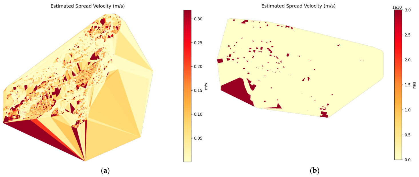
Figure 5 presents the estimated fire spread velocity in m/s, derived from the spatial gradient of the kriging-interpolated arrival-time surface. For each triangulated face in the Delaunay mesh connecting kriged grid points, the velocity is computed as the inverse of the arrival-time gradient magnitude: v = 1/|grad(A)|, where A(x,y) is the arrival time. The resulting map reveals the fine-scale spatial heterogeneity of fire spread that aggregate statistics (Table 6) cannot capture. High-velocity regions (dark red, exceeding 0.14 m/s) correspond to wind-driven runs through continuous, receptive fuels; these corridors are often aligned with the dominant wind direction visible in the wind rose (Figure 3b). Low-velocity regions (pale yellow, below 0.02 m/s) indicate areas where the fire crept slowly through sparse fuels, encountered terrain barriers, or burned against the wind.

Comparing spread velocity maps across events from different fire regimes reveals fundamentally different spatial patterns. Wind-driven Mediterranean events (e.g., Evia 2021, Evros 2023) exhibit broad swaths of high-velocity spread aligned with the Etesian wind corridor, punctuated by narrow low-velocity bands at ridgelines. In contrast, terrain-controlled montane events (e.g., Cameron Peak 2020, Cedar Creek 2022) show a patchwork of velocity extremes dictated by slope aspect, canyon channeling, and fuel discontinuities. These maps demonstrate that fire behavior operates at spatial scales well below the 1 km resolution of existing benchmark datasets, validating WildfireCube’s 30 m resolution as necessary for capturing the physical mechanisms governing spread variability. The velocity field also serves as a derived training target for ML models: rather than predicting binary spread alone, models can learn to regress continuous spread velocity, enabling physically meaningful evaluation metrics such as velocity RMSE and directional accuracy.

9.2. Fire Radiative Power Analysis

Fire Radiative Power (FRP, in MW), reported by FIRMS as the instantaneous thermal energy release rate, provides a fire-intensity signal independent of the spatial interpolation used to reconstruct arrival times. Across the 13 events, mean FRP ranges from 33.6 MW (Carr) to 78.1 MW (East Troublesome), with a catalog-wide mean of 50.7 MW. The maximum single-detection FRP spans an order of magnitude, from 1615 MW (Eagle Creek) to 16,146 MW (East Troublesome). The extreme FRP maximum at East Troublesome reflects the October 2020 wind-driven run that produced a “fire tornado” and crossed the Continental Divide in a single night; the high specific energy release is consistent with rapid combustion of dry lodgepole pine and spruce-fir litter in strong downslope wind. Elephant Hill ranks second in mean FRP (68.3 MW) despite its smaller burned area, reflecting the high-intensity behavior characteristic of boreal fires where continuous surface and crown fuels support sustained combustion. Total FIRMS detections vary across three orders of magnitude, from 948 (Eagle Creek, severely overpass-limited) to 39,791 (Creek, a 13-day California event with dense VIIRS revisit coverage). The catalog contains 178,268 hotspot detections in total.

9.3. Weather Regime Analysis

Mean 2 m air temperature ranges from 2.47 °C (East Troublesome) to 29.18 °C (Evia), spanning a 26.7 °C band from alpine autumn to peak Mediterranean summer. Maximum instantaneous wind speed across the event domain ranges from 3.39 m/s (Cedar Creek) to 11.02 m/s (Calf Canyon/Hermits Peak), with a catalog mean of 5.33 m/s. Two distinct weather regimes emerge. The temperature-driven cluster (Evia, Evros, Carr, Dixie, Bootleg; mean temp > 23 °C) is characterized by sustained heat that reduces live fuel moisture to critical thresholds, enabling sustained ignition and crown fire transition. The wind-driven cluster (East Troublesome, Calf Canyon/Hermits Peak, Evros) is distinguished by maximum wind speeds exceeding 7 m/s, reflecting downslope and Etesian wind systems that dominate spread rate regardless of temperature. Evros occupies both clusters simultaneously—high temperature (25.8 °C) and maximum wind (9.10 m/s)—consistent with the compound fire weather that drove its exceptional 188.44 km² burned area. The FWI proxy mean ranges from 6.4 (Elephant Hill) to 20.0 (Bootleg), and the maximum instantaneous FWI proxy reaches 75.5 at Calf Canyon/Hermits Peak, reflecting the exceptional spring 2022 drought and wind event in New Mexico.

9.4. Burn Severity Analysis

The high-severity fraction (pixels with RBR > 0.27, indicating crown fire or severe surface fire) ranges from 0.1% (Dixie) to 31.5% (Elephant Hill), with a catalog mean of 15.5%. Elephant Hill (31.5%), Evia (31.1%), and Bootleg (28.3%) exhibit the highest high-severity fractions, all three burning through dense, continuous conifer or pine canopy that supports deep-burning fire with complete crown consumption. Dixie (0.1%) and Eagle Creek (1.0%) show the lowest high-severity fractions; in both cases, the RBR channel is heavily contaminated by pathological denominator values over sparse or non-vegetated terrain. For the five events with reliable RBR (positive mean RBR: Bootleg, Evia, Calf Canyon/Hermits Peak, Cedar Creek, Cameron Peak), the high-severity fraction is a physically meaningful metric available for severity regression tasks. For the remaining eight events, the per-pixel dNBR channel provides a more robust severity signal that is not affected by the denominator instability of RBR.

9.5. Terrain and Elevation Analysis

The 13 events sample an elevation range from near sea level (Evros, mean 162 m) to sub-alpine terrain (East Troublesome, mean 2853 m; Cameron Peak, mean 2543 m). The burned-area elevation is consistently higher than the full-domain mean for most North American events—Calf Canyon/Hermits Peak (burned 2628 m vs. domain 2468 m) and Cameron Peak (burned 2880 m vs. 2543 m)—reflecting the tendency of mountain fires to spread upslope through dense mid-elevation forest before encountering sub-alpine fuels. Mediterranean events show the inverse pattern: Evia’s fire burned at lower elevations (195 m) than the domain average (154 m) because the island’s higher terrain was both less vegetated and less accessible to the coastline-initiated spread.

9.6. Aggregate Dataset Statistics

Table 8 summarizes the catalog-wide aggregate statistics computed across all 13 processed wildfire events, reporting the minimum, maximum, mean, and median of each metric, together with the cumulative total where a quantity is summable across events. These figures characterize the overall scale and variability of the assembled WildfireCube dataset.

Table 8. Catalog-wide aggregate statistics across all 13 processed events. -- indicates metrics not summable across events.

Metric	Min	Max	Mean	Median	Total (13 Events)
Burned area (km2)	13.34	188.44	66.08	42.73	859.04
Burned fraction (%)	0.32	8.63	2.03	1.10	--
Duration (days)	10	15	13.5	14	175
Timesteps (T)	80	120	107.7	112	1400
FIRMS detections	948	39,791	13,713	10,891	178,268
Mean FRP (MW)	33.6	78.1	50.7	48.8	--
Max FRP (MW)	1615	16,146	6553	5617	--
Mean wind (m/s)	1.14	3.88	2.02	1.70	--
Max wind (m/s)	3.39	11.02	5.33	4.53	--
Mean temperature (°C)	2.47	29.18	19.53	19.78	--
FWI proxy mean	6.4	20.0	10.3	9.4	--
FWI proxy max	17.5	75.5	38.5	39.3	--
Max spread (km2/3 h)	2.80	150.75	42.96	37.34	--
High severity (%)	0.1	31.5	15.5	19.2	--

Table 8. Catalog-wide aggregate statistics across all 13 processed events. -- indicates metrics not summable across events.

Metric	Min	Max	Mean	Median	Total (13 Events)
Burned area (km2)	13.34	188.44	66.08	42.73	859.04
Burned fraction (%)	0.32	8.63	2.03	1.10	--
Duration (days)	10	15	13.5	14	175
Timesteps (T)	80	120	107.7	112	1400
FIRMS detections	948	39,791	13,713	10,891	178,268
Mean FRP (MW)	33.6	78.1	50.7	48.8	--
Max FRP (MW)	1615	16,146	6553	5617	--
Mean wind (m/s)	1.14	3.88	2.02	1.70	--
Max wind (m/s)	3.39	11.02	5.33	4.53	--
Mean temperature (°C)	2.47	29.18	19.53	19.78	--
FWI proxy mean	6.4	20.0	10.3	9.4	--
FWI proxy max	17.5	75.5	38.5	39.3	--
Max spread (km2/3 h)	2.80	150.75	42.96	37.34	--
High severity (%)	0.1	31.5	15.5	19.2	--

9.7. Dataset Scale and Storage

The 13-event processed catalog represents a substantial geospatial dataset. After zstd recompression with bitshuffle pre-filtering (Section 7), the compressed Zarr stores for all 13 events collectively exceed 300 GB, including both raw (12-channel) and normalized (13-channel) tensor variants. The total logical (uncompressed) size exceeds 800 GB given the 2.58× compression ratio demonstrated on representative events. Table 9 provides a breakdown of the dataset at the catalog level.

Table 9. Dataset scale summary for the WildfireCube catalog. The full event catalog is projected to exceed 2 TB of raw float32 tensor data before compression.

Dimension	Value (13-Event Catalog)
Events processed	13
Target catalog size	40 events
Total event days	175 days
Total temporal bins (3 h)	1400 timesteps
Total FIRMS detections	178,268
Total burned area	859.04 km2
Spatial resolution	30 m (UTM)
Temporal resolution	3 h
Channels per tensor (raw)	12
Channels per tensor (normalized)	13
Chunk size	(1, 12, 256, 256) = ~3 MB uncompressed
Compressed storage (13 events)	>300 GB (zstd + bitshuffle)
Projected full catalog	>2 TB raw data
Compression ratio (zstd + bitshuffle)	2.58× vs. float32 baseline

Table 9. Dataset scale summary for the WildfireCube catalog. The full event catalog is projected to exceed 2 TB of raw float32 tensor data before compression.

Dimension	Value (13-Event Catalog)
Events processed	13
Target catalog size	40 events
Total event days	175 days
Total temporal bins (3 h)	1400 timesteps
Total FIRMS detections	178,268
Total burned area	859.04 km2
Spatial resolution	30 m (UTM)
Temporal resolution	3 h
Channels per tensor (raw)	12
Channels per tensor (normalized)	13
Chunk size	(1, 12, 256, 256) = ~3 MB uncompressed
Compressed storage (13 events)	>300 GB (zstd + bitshuffle)
Projected full catalog	>2 TB raw data
Compression ratio (zstd + bitshuffle)	2.58× vs. float32 baseline

9.8. ML Readiness and Benchmark Design

All processed events are assembled into standardized (T, C, H, W) tensor format, with both raw (12-channel, physical units) and normalized (13-channel, bounded) variants stored as Zarr arrays. This uniformity enables direct ingestion by convolutional, recurrent, and attention-based architectures without per-event preprocessing. The channel layout operationalizes the teacher-forced dynamical system, ensuring that the separation of causal roles is preserved identically across all events so that any learned function applies consistently regardless of geographic context.

Class balance is the principal challenge for downstream ML training: burned pixels constitute between 0.32% and 8.63% of each event’s spatial domain. Effective training will require focal loss, inverse-frequency weighting, or spatial sampling strategies that oversample the fire-front neighborhood. Once the full catalog is assembled, events can be split along three meaningful axes: (i) geographic—North American training/Greek out-of-distribution testing; (ii) fire-regime—leave-one-regime-out cross-validation across Mediterranean, boreal, alpine, chaparral, and montane folds; and (iii) temporal—2016–2021 training/2022–2024 held-out test, simulating operational deployment where future fire behavior must be predicted from historically learned patterns. The tensor structure supports multiple prediction tasks: binary spread (fire-front mask channel), severity regression (RBR channel), cumulative burn (fractional burn channel), and multi-step autoregressive rollout evaluation.

9.9. Novelty and Value Proposition

WildfireCube makes several contributions that distinguish it from existing wildfire ML datasets. We summarize these advances and their practical significance relative to the literature reviewed in Section 2.

Resolution. WildfireCube operates at 30 m spatial and 3 h temporal resolution, representing an order-of-magnitude improvement over the most widely used benchmarks. The Next Day Wildfire Spread dataset [4] provides 1 km/daily data; WildfireSpreadTS [5] offers 375 m/daily; the Canadian Fire Spread Dataset [9] operates at 180 m/daily; and SeasFire [8] at 0.25 degree/8 days. At 30 m, WildfireCube resolves individual firebreaks, road networks, riparian corridors, and fuel transitions that are invisible at coarser scales. The 3 h temporal cadence captures diurnal fire behavior cycles, including the characteristic afternoon wind-driven spread and nocturnal backing fire patterns that daily datasets fundamentally cannot represent.

Physics-informed normalization. No existing wildfire or Earth-observation dataset applies a physics-informed normalization scheme with fixed physical bounds. Standard practice normalizes channels using sample statistics (min-max or z-score computed from training data), which introduces distributional assumptions and prevents exact inversion to physical units. WildfireCube instead maps each channel using domain-specific physical constants (e.g., temperature clipped to [−5, 45] °C and affine-rescaled, wind components divided by a 15 m/s fire-weather threshold, slope divided by its 90-degree physical maximum), ensuring that normalized values are interpretable, cross-event comparable, and exactly invertible. This is a genuinely novel contribution with no published precedent in the wildfire or remote-sensing literature.

Causal channel structure. The explicit separation of channels into static landscape controls (S), dynamic atmospheric forcings (D), and evolving fire state (Y) operationalizes the teacher-forced dynamical system formulation Y_t+1 = F(Y_t, D_t+1, S). This causal decomposition is preserved identically across all events, enabling models to learn physically meaningful relationships between weather, terrain, and fire behavior. While other datasets include similar variable types, WildfireCube is the first to enforce a strict causal ordering in the channel layout as part of the data specification itself.

Multi-regime coverage. Existing wildfire datasets typically focus on a single geographic region or fire regime: the Next Day Wildfire Spread dataset covers the contiguous US, Mesogeos [6] covers the Mediterranean, and the Canadian Fire Spread Dataset [9] covers boreal Canada. Even the 13 demonstration events already span six distinct fire-regime categories (Mediterranean scrubland, Pacific Northwest dense forest, California chaparral, boreal forest, alpine/montane, and semi-arid grassland–forest transitions) across three countries within a single harmonized tensor format. The full event catalog will extend this further, providing the multi-regime diversity essential for training models that generalize across fundamentally different fuel structures, topographic settings, and meteorological forcing patterns.

Data quality over model complexity. The finding by Di Giuseppe et al. [16] that data quality matters more than model complexity for fire prediction provides strong motivation for the WildfireCube approach. Rather than proposing a novel architecture, this work invests in the upstream data engineering that determines the ceiling on any downstream model’s performance: careful multi-source fusion at native resolution, physics-based normalization, quality-controlled fire-state reconstruction via kriging, and systematic data validation through per-event analytical reports.

10. Conclusions

We have presented WildfireCube, a reproducible pipeline and methodology for constructing dense spatiotemporal wildfire tensors at 30 m spatial and 3 h temporal resolution. The pipeline fuses four freely available remote-sensing and reanalysis products into a physically structured (T, 13, H, W) tensor that separates static landscape controls, dynamic atmospheric forcings, and evolving fire state into causally distinct channel groups. A physics-informed normalization framework maps all channels to bounded, interpretable numeric ranges using fixed physical constants, enabling cross-event transfer and exact inversion to physical units. Zarr-based chunked storage with Zstandard compression and bitshuffle pre-filtering achieves a 2.58× compression ratio and reduces total disk footprint by over 60%.

We demonstrated the pipeline on 13 wildfire events across the United States, Canada, and Greece, spanning a 14-fold range in burned area and six distinct fire regimes. The demonstration runs validate the pipeline’s ability to handle diverse terrain types (from sea-level Mediterranean scrubland to sub-alpine conifer forests), fire behavior patterns (from slow terrain-controlled creep to explosive wind-driven runs), and data availability conditions (from dense FIRMS detection fields to sparse peripheral observations). The per-event analytical reports produced by the pipeline provide comprehensive quality assessment and cross-event comparison, confirming that the tensor representation faithfully captures the physical drivers of fire spread.

The primary direction for future work is producing a large-scale, multi-regime dataset suitable for training deep learning models for spatiotemporal wildfire spread prediction. With the pipeline fully automated and each event specified by a single YAML configuration file, scaling from 13 to any number of events requires no methodological changes. The resulting dataset, projected to exceed 2 TB of raw data, will provide the scale and diversity needed to train and rigorously evaluate convolutional, recurrent, and attention-based architectures on the teacher-forced autoregressive prediction task defined by the tensor’s causal channel structure.

Beyond catalog expansion, several additional extensions are planned. Temporal resolution could be increased by incorporating geostationary satellite observations (GOES-16/17, MSG/Meteosat), providing sub-hourly detections. Incorporation of live and dead fuel moisture content from ERA5-Land soil moisture would add a critical mechanistic variable currently absent. Finally, integration with physics-based spread models such as FARSITE or PHOENIX would enable hybrid ML-physics architectures that combine statistical flexibility with physical constraints.