Author Contributions
Conceptualization, J.Y., J.L., S.L., G.J. and S.-H.L.; methodology, J.Y., J.L., S.L., G.J., J.P. and W.J.; software, J.Y., S.L., G.J., J.P. and W.J.; validation, J.Y., S.L., G.J. and J.P.; formal analysis, J.Y., S.L., G.J. and J.P.; investigation, J.Y., J.L., S.L., G.J., J.P. and W.J.; resources, S.-H.L., C.L., C.-W.L., C.-W.O. and S.-Y.K.; data curation, J.Y., S.L., G.J., J.P. and W.J.; writing—original draft preparation, J.Y.; writing—review and editing, J.Y. and J.L.; visualization, J.Y., S.L., G.J. and J.P.; supervision, J.L., S.-H.L. and S.-O.P.; project administration, J.L., S.-H.L., C.L., C.-W.L., C.-W.O., S.-Y.K. and S.-O.P.; funding acquisition, S.-H.L., C.L., C.-W.L., C.-W.O., S.-Y.K. and S.-O.P. All authors have read and agreed to the published version of the manuscript.
Figure 1.
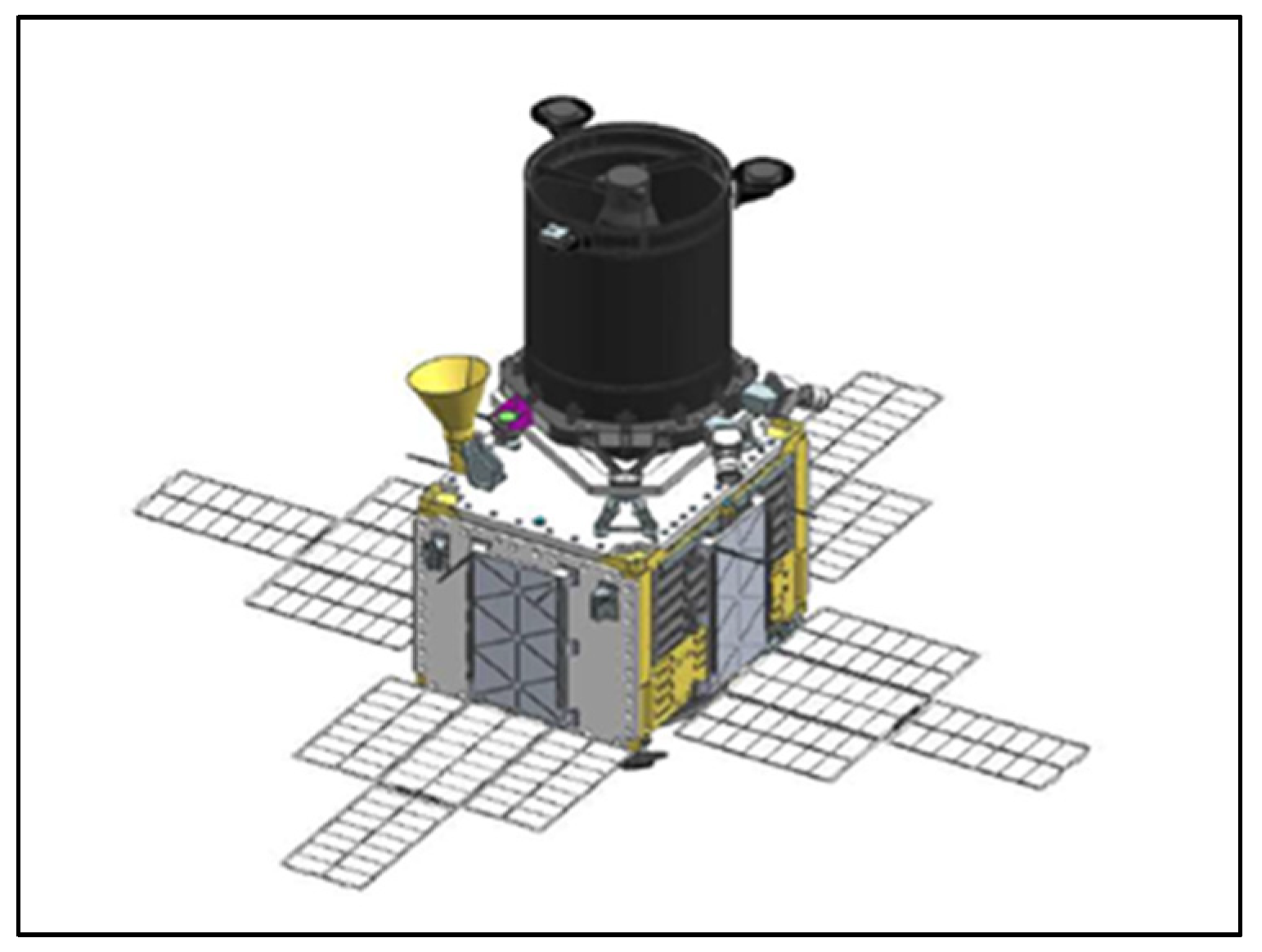
The flight model of NEONSAT.
Figure 1.
The flight model of NEONSAT.
Figure 2.
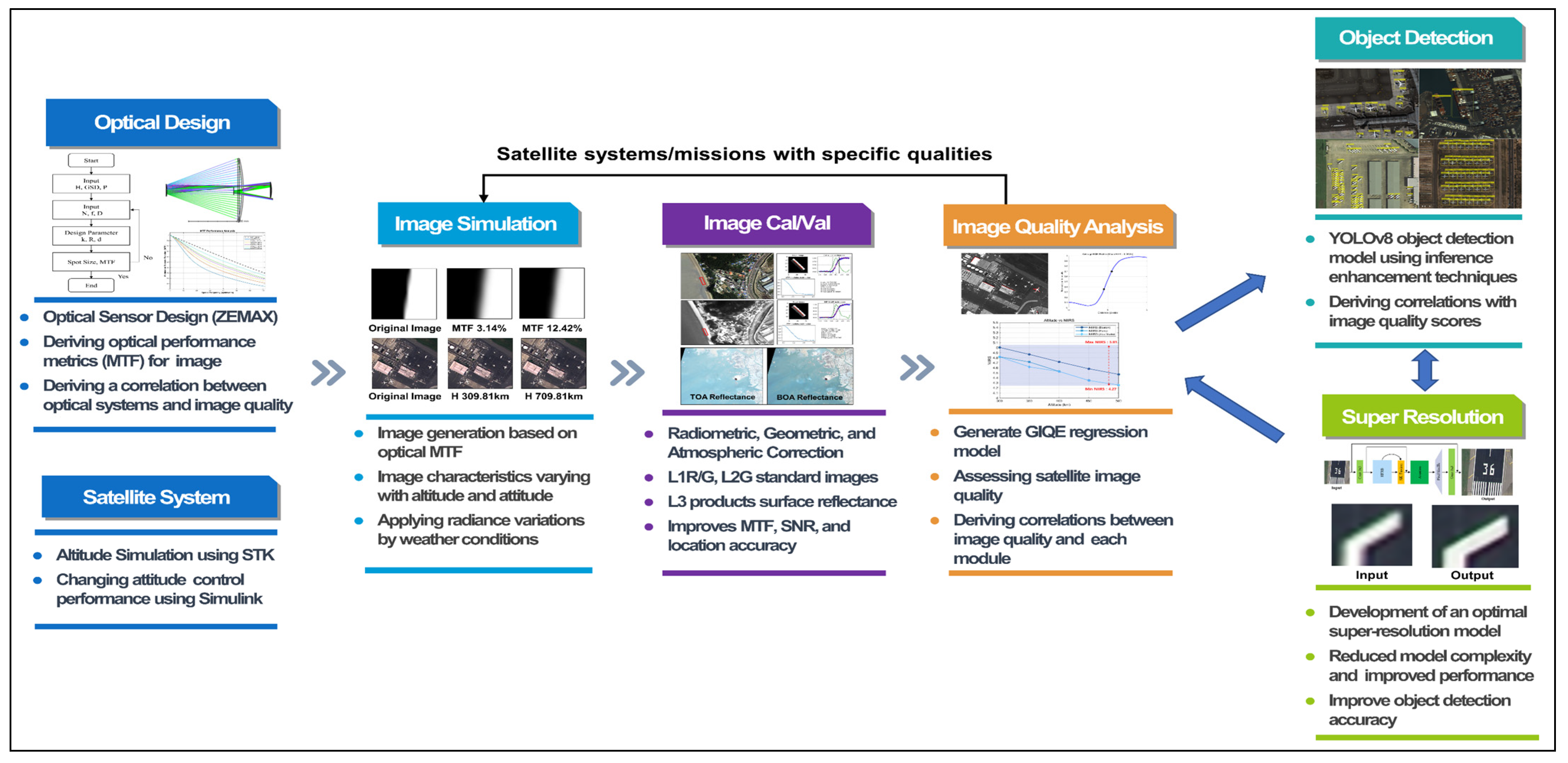
Integrated framework used in this study for spatial image quality assessment. The framework links optical design analysis, image simulation, GIQE-based NIIRS assessment, object detection performance, and super-resolution analysis using NEONSAT imagery and representative simulations.
Figure 2.
Integrated framework used in this study for spatial image quality assessment. The framework links optical design analysis, image simulation, GIQE-based NIIRS assessment, object detection performance, and super-resolution analysis using NEONSAT imagery and representative simulations.
Figure 3.
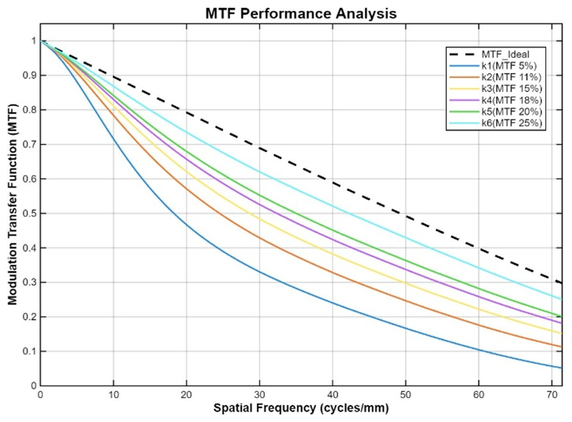
Optical modulation transfer function, , as a function of spatial frequency for the selected optical cases. The conic constant was adjusted in Zemax so that the MTF at the Nyquist frequency corresponded to 5, 11, 15, 18, 20, and 25%.
Figure 3.
Optical modulation transfer function, , as a function of spatial frequency for the selected optical cases. The conic constant was adjusted in Zemax so that the MTF at the Nyquist frequency corresponded to 5, 11, 15, 18, 20, and 25%.
Figure 4.
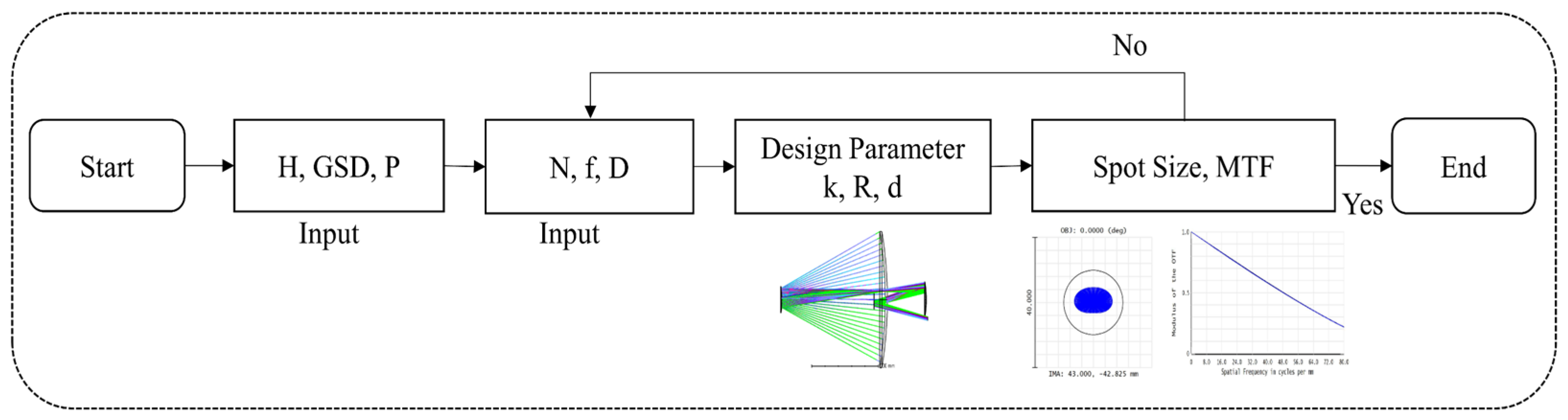
Optical design analysis flow based on the baseline NEONSAT payload configuration. The conic constant was varied in Zemax to generate a set of conditions for subsequent image simulation.
Figure 4.
Optical design analysis flow based on the baseline NEONSAT payload configuration. The conic constant was varied in Zemax to generate a set of conditions for subsequent image simulation.
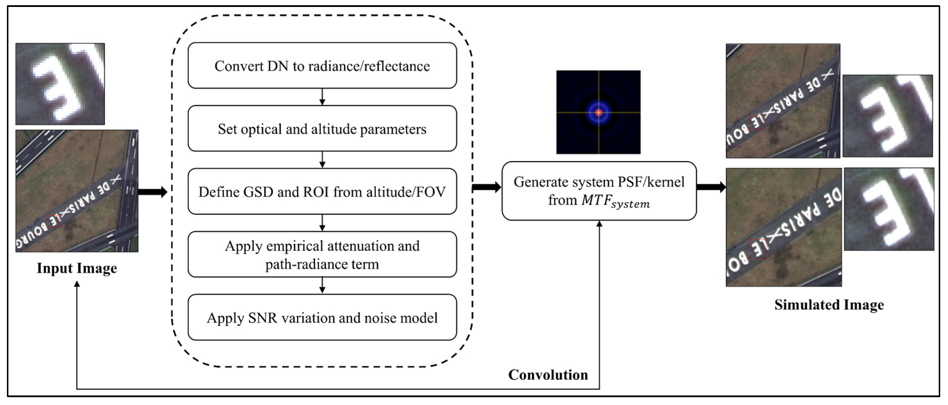
Figure 5.
Image simulation procedure used in this study. The cases derived from Zemax were propagated through the pyBSM-based imaging chain to construct using detector and atmospheric MTF components. GSD sampling, empirical attenuation and path radiance terms, and simplified relative SNR scaling were applied as simulation conditions to generate simulated images under controlled image-quality conditions.
Figure 5.
Image simulation procedure used in this study. The cases derived from Zemax were propagated through the pyBSM-based imaging chain to construct using detector and atmospheric MTF components. GSD sampling, empirical attenuation and path radiance terms, and simplified relative SNR scaling were applied as simulation conditions to generate simulated images under controlled image-quality conditions.
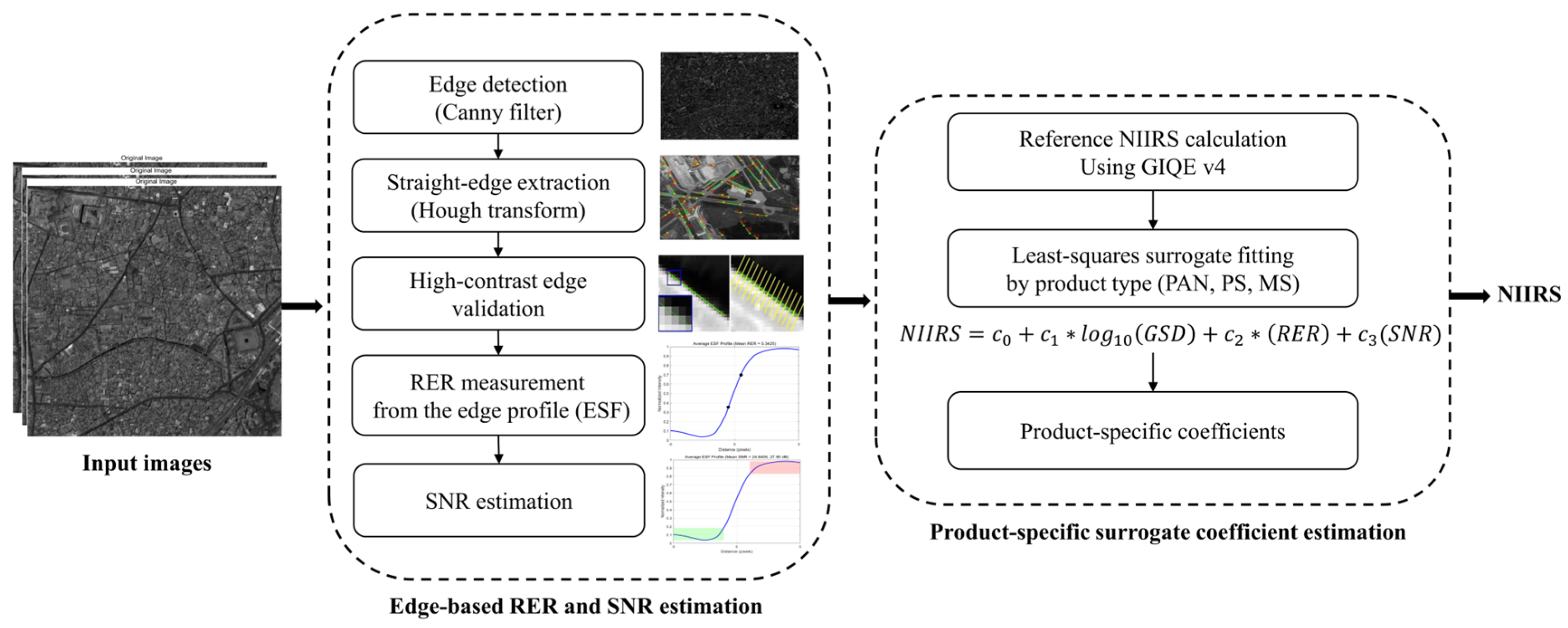
Figure 6.
Workflow of the GIQE-based NIIRS assessment used in this study. The procedure includes edge detection and screening, RER and SNR estimation from natural targets, reference NIIRS calculation using GIQE v4, and product-specific least-squares surrogate fitting for PAN, PS, and MS products. Representative intermediate images are shown only to illustrate the processing steps, whereas the fitted coefficients are reported quantitatively in
Table 3.
Figure 6.
Workflow of the GIQE-based NIIRS assessment used in this study. The procedure includes edge detection and screening, RER and SNR estimation from natural targets, reference NIIRS calculation using GIQE v4, and product-specific least-squares surrogate fitting for PAN, PS, and MS products. Representative intermediate images are shown only to illustrate the processing steps, whereas the fitted coefficients are reported quantitatively in
Table 3.
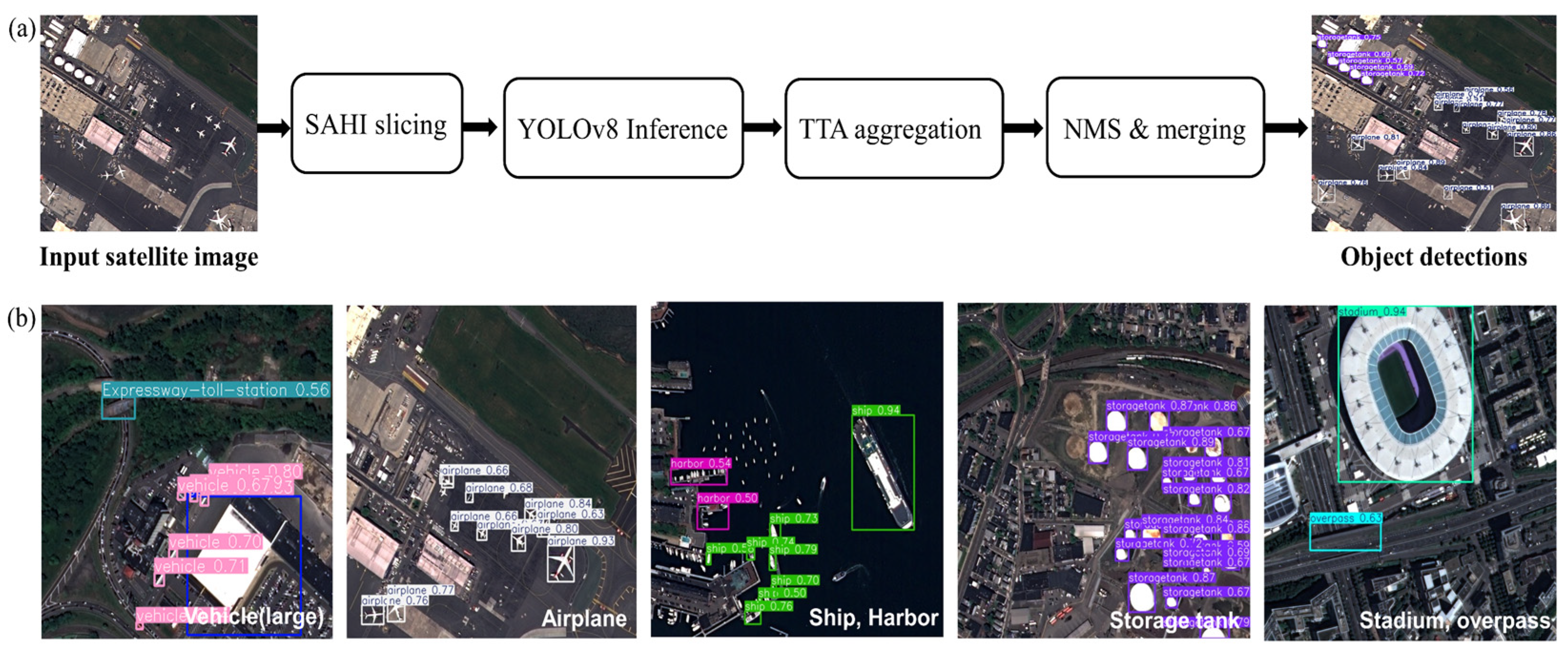
Figure 7.
Object detection module used in this study: (a) workflow of object detection, including SAHI-based slicing, YOLOv8 inference, test-time augmentation, and final prediction merging; (b) representative detection examples from NEONSAT-1 image chips used for subsequent comparison.
Figure 7.
Object detection module used in this study: (a) workflow of object detection, including SAHI-based slicing, YOLOv8 inference, test-time augmentation, and final prediction merging; (b) representative detection examples from NEONSAT-1 image chips used for subsequent comparison.
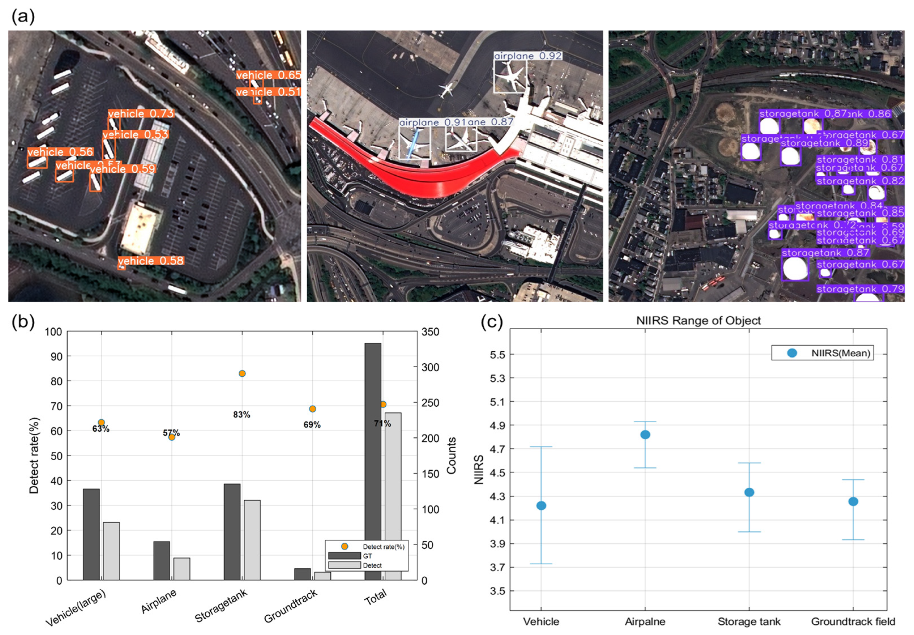
Figure 8.
Object detection and NIIRS results for the NEONSAT-1 PS product over Boston Logan International Airport: (a) representative detected targets; (b) detection rate for each target type, with ground-truth and detected object counts; (c) NIIRS range for each target type.
Figure 8.
Object detection and NIIRS results for the NEONSAT-1 PS product over Boston Logan International Airport: (a) representative detected targets; (b) detection rate for each target type, with ground-truth and detected object counts; (c) NIIRS range for each target type.
Figure 9.
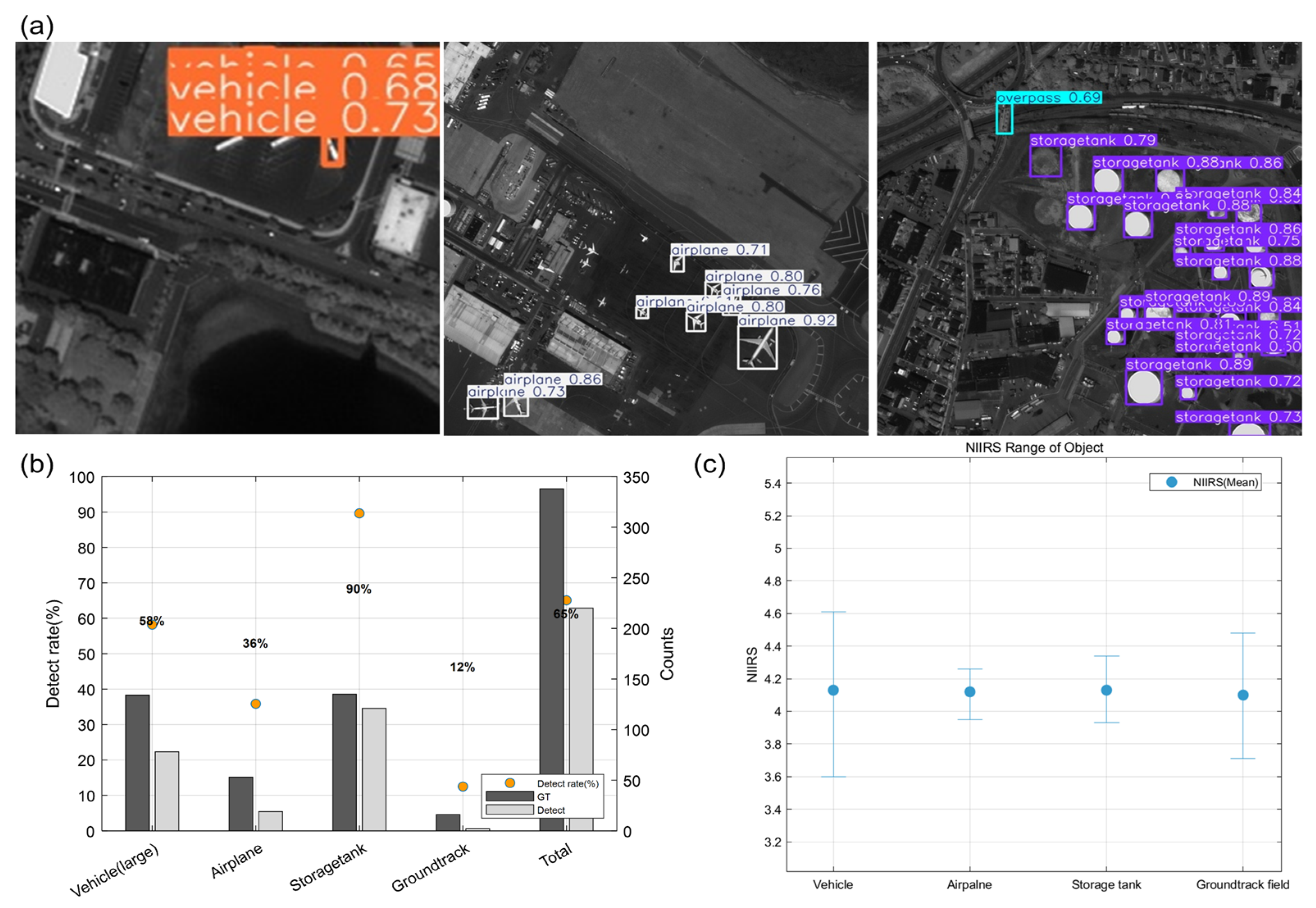
Object detection and NIIRS results for the NEONSAT-1 PAN product over Boston Logan International Airport: (a) representative detected targets; (b) detection rate for each target type, with ground-truth and detected object counts; (c) NIIRS range for each target type.
Figure 9.
Object detection and NIIRS results for the NEONSAT-1 PAN product over Boston Logan International Airport: (a) representative detected targets; (b) detection rate for each target type, with ground-truth and detected object counts; (c) NIIRS range for each target type.
Figure 10.
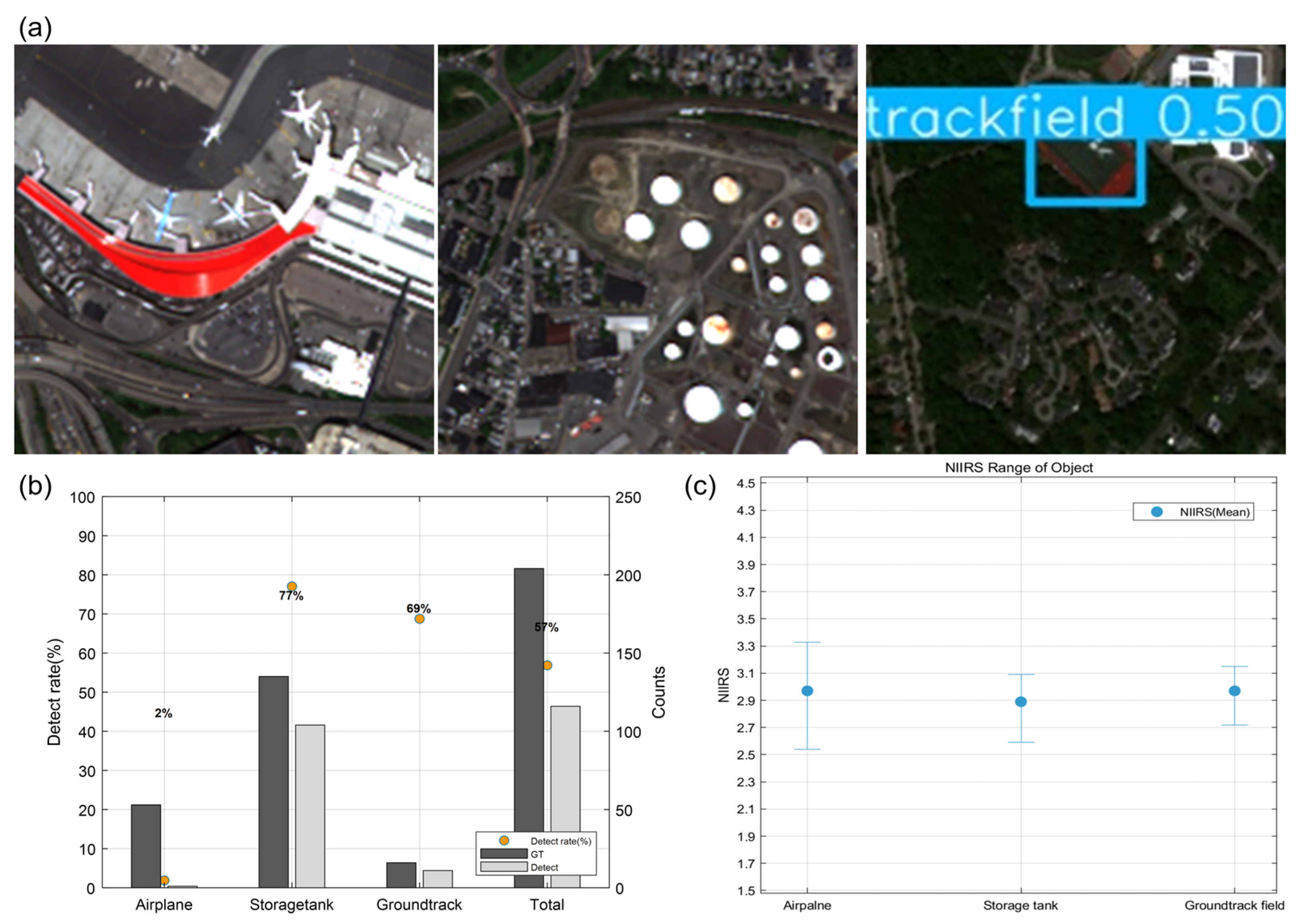
Object detection and NIIRS results for the NEONSAT-1 MS product over Boston Logan International Airport: (a) representative detected targets; (b) detection rate for each target type, with ground-truth and detected object counts; (c) NIIRS range for each target type.
Figure 10.
Object detection and NIIRS results for the NEONSAT-1 MS product over Boston Logan International Airport: (a) representative detected targets; (b) detection rate for each target type, with ground-truth and detected object counts; (c) NIIRS range for each target type.
Figure 11.
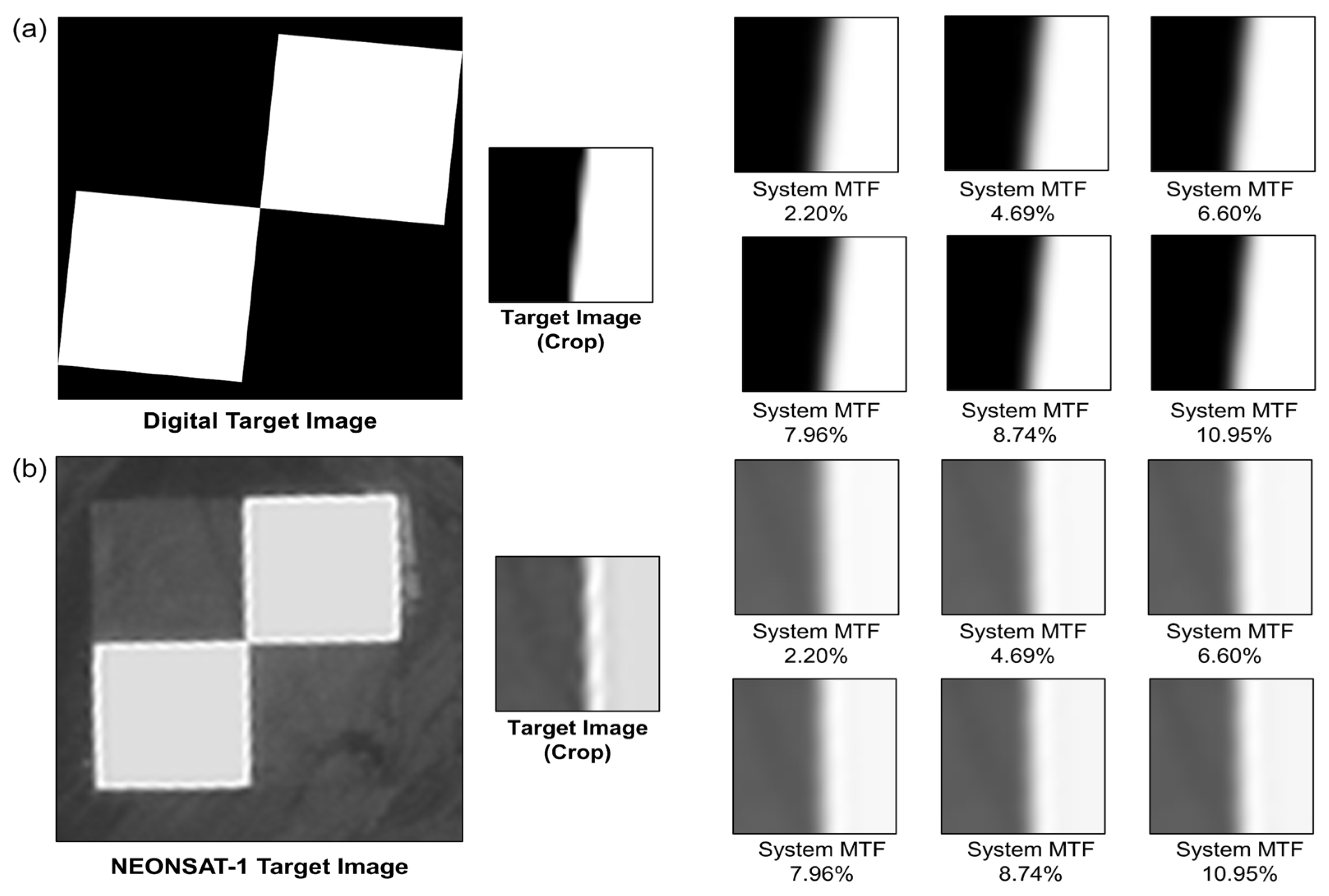
Edge-response examples under controlled conditions: (a) an ideal digital edge target; (b) a real NEONSAT edge target. In both targets, increasing sharpens the edge transition, although the visual difference is more evident in the digital target than in the observed target.
Figure 11.
Edge-response examples under controlled conditions: (a) an ideal digital edge target; (b) a real NEONSAT edge target. In both targets, increasing sharpens the edge transition, although the visual difference is more evident in the digital target than in the observed target.
Figure 12.
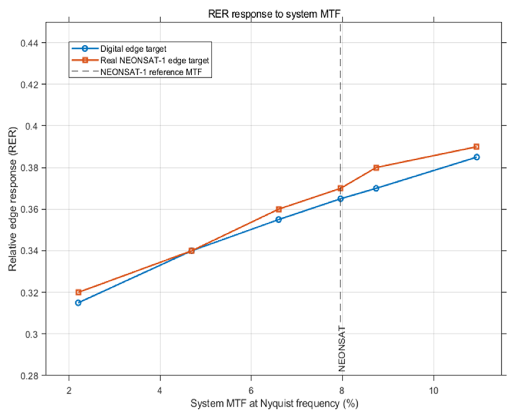
RER as a function of for the digital and real edge targets. The digital target shows a smoother response to the controlled sharpness variation, whereas the real target exhibits a more scattered trend because observed scene heterogeneity is superimposed on the edge response.
Figure 12.
RER as a function of for the digital and real edge targets. The digital target shows a smoother response to the controlled sharpness variation, whereas the real target exhibits a more scattered trend because observed scene heterogeneity is superimposed on the edge response.
Figure 13.
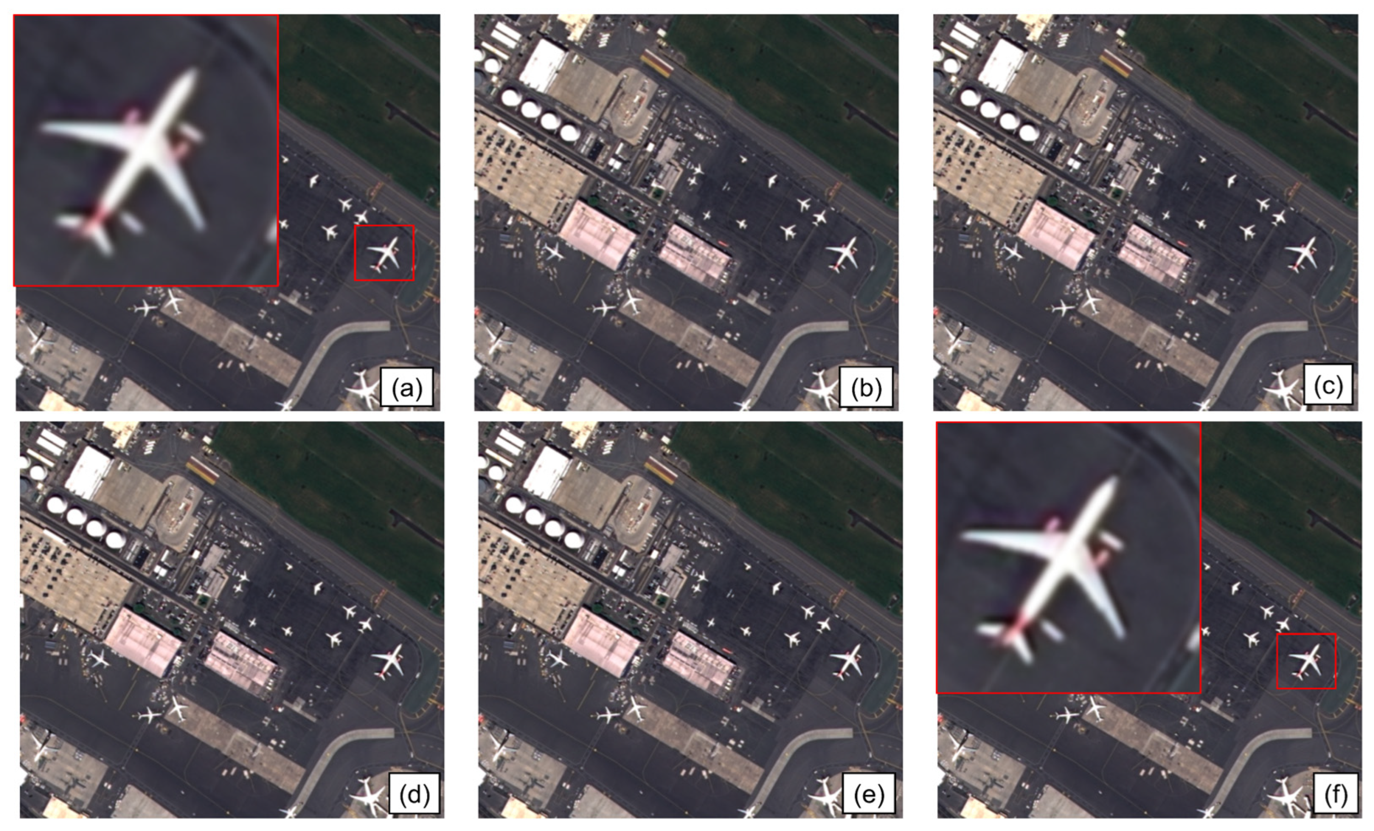
Boston PS scene under different conditions: (a) ; (b) ; (c) ; (d) ; (e) ; (f) ; The figure illustrates the visual response of the NEONSAT-1 image chip and representative detected targets as increases.
Figure 13.
Boston PS scene under different conditions: (a) ; (b) ; (c) ; (d) ; (e) ; (f) ; The figure illustrates the visual response of the NEONSAT-1 image chip and representative detected targets as increases.
Figure 14.
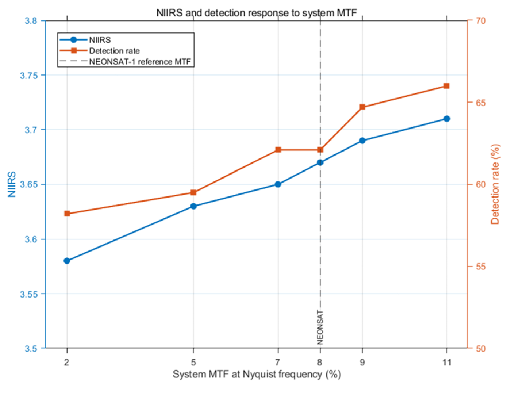
NIIRS and detection rate as functions of for the Boston PS scene. Both metrics increase with over the tested range, indicating that controlled sharpness variation is reflected in downstream object detection performance.
Figure 14.
NIIRS and detection rate as functions of for the Boston PS scene. Both metrics increase with over the tested range, indicating that controlled sharpness variation is reflected in downstream object detection performance.
Figure 15.
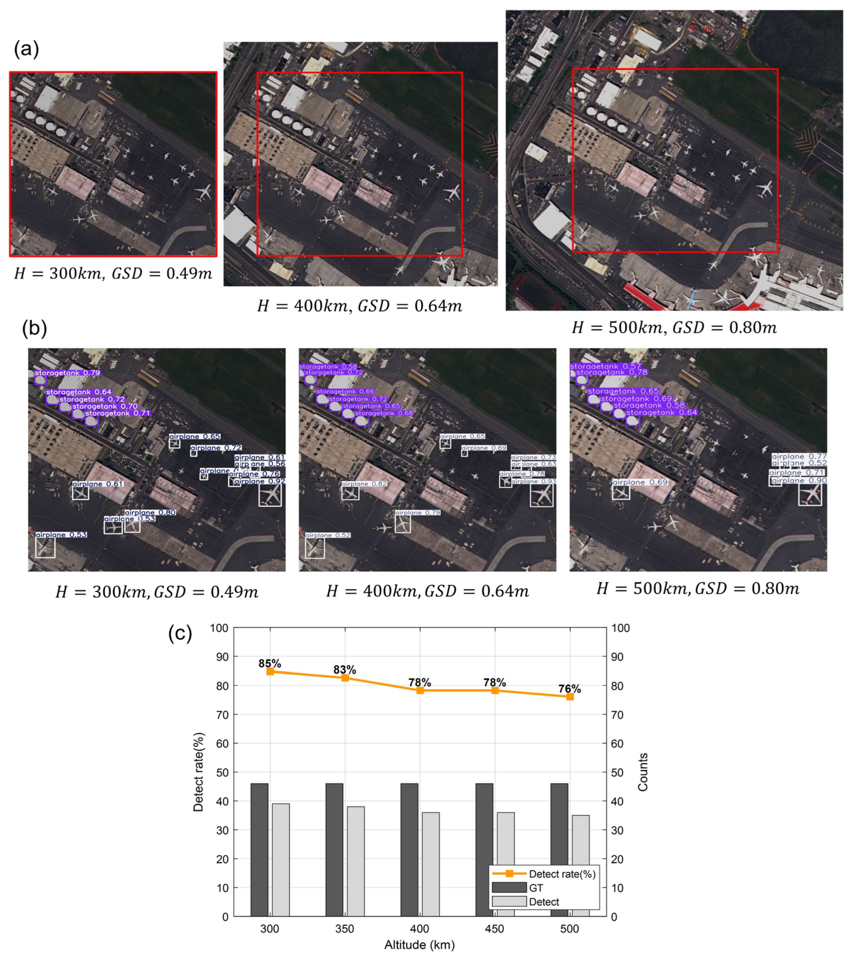
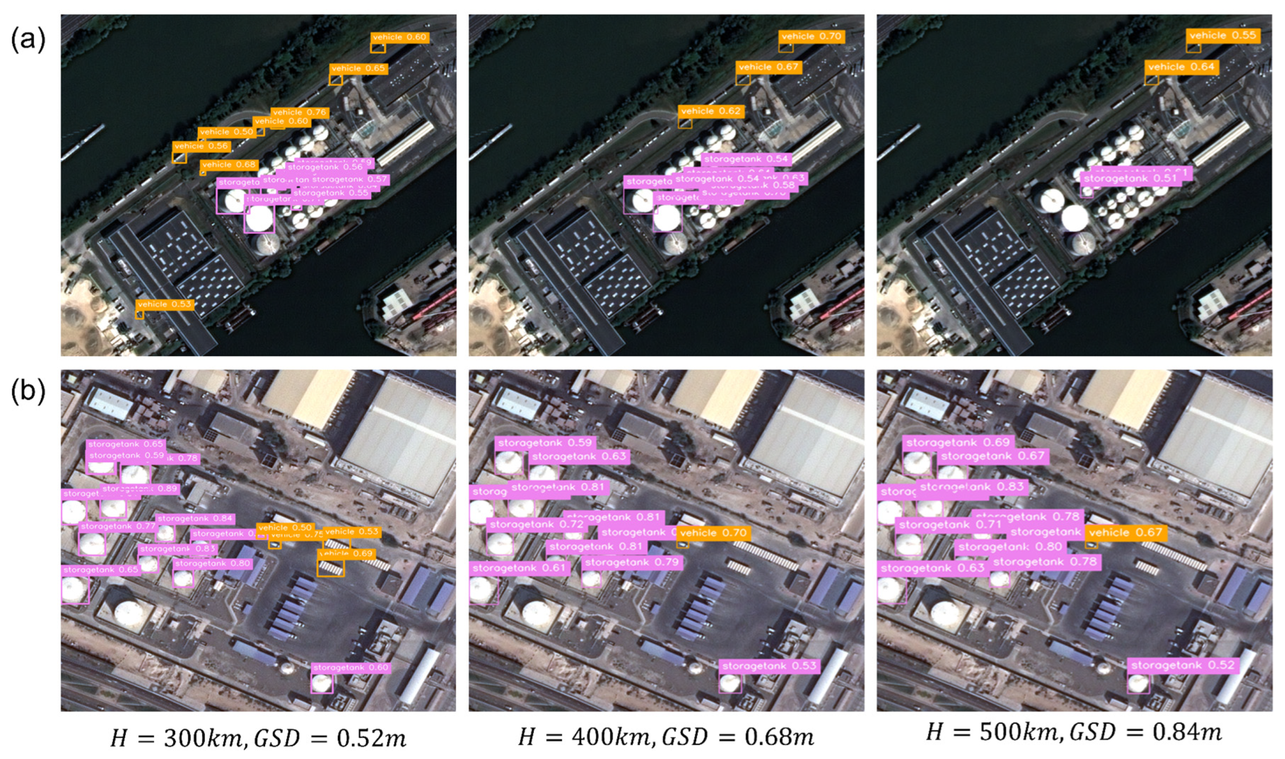
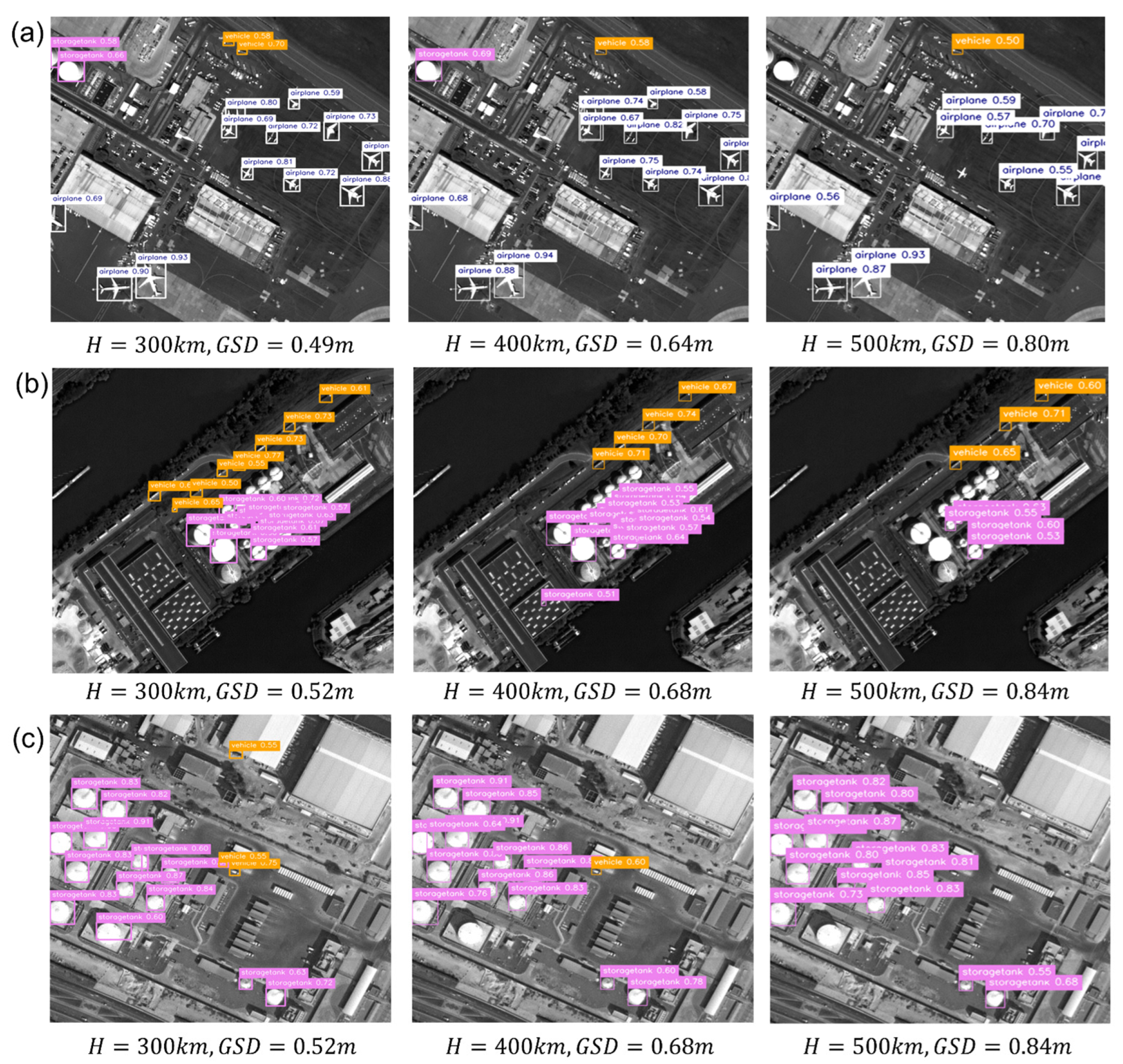
Altitude-dependent simulation results for the Boston PS scene: (a) image chips at different altitudes and corresponding GSDs, where the red box denotes the reference region defined at 300 km; (b) detection outputs for the same region; (c) detection rate and object count as a function of altitude.
Figure 15.
Altitude-dependent simulation results for the Boston PS scene: (a) image chips at different altitudes and corresponding GSDs, where the red box denotes the reference region defined at 300 km; (b) detection outputs for the same region; (c) detection rate and object count as a function of altitude.
Figure 16.
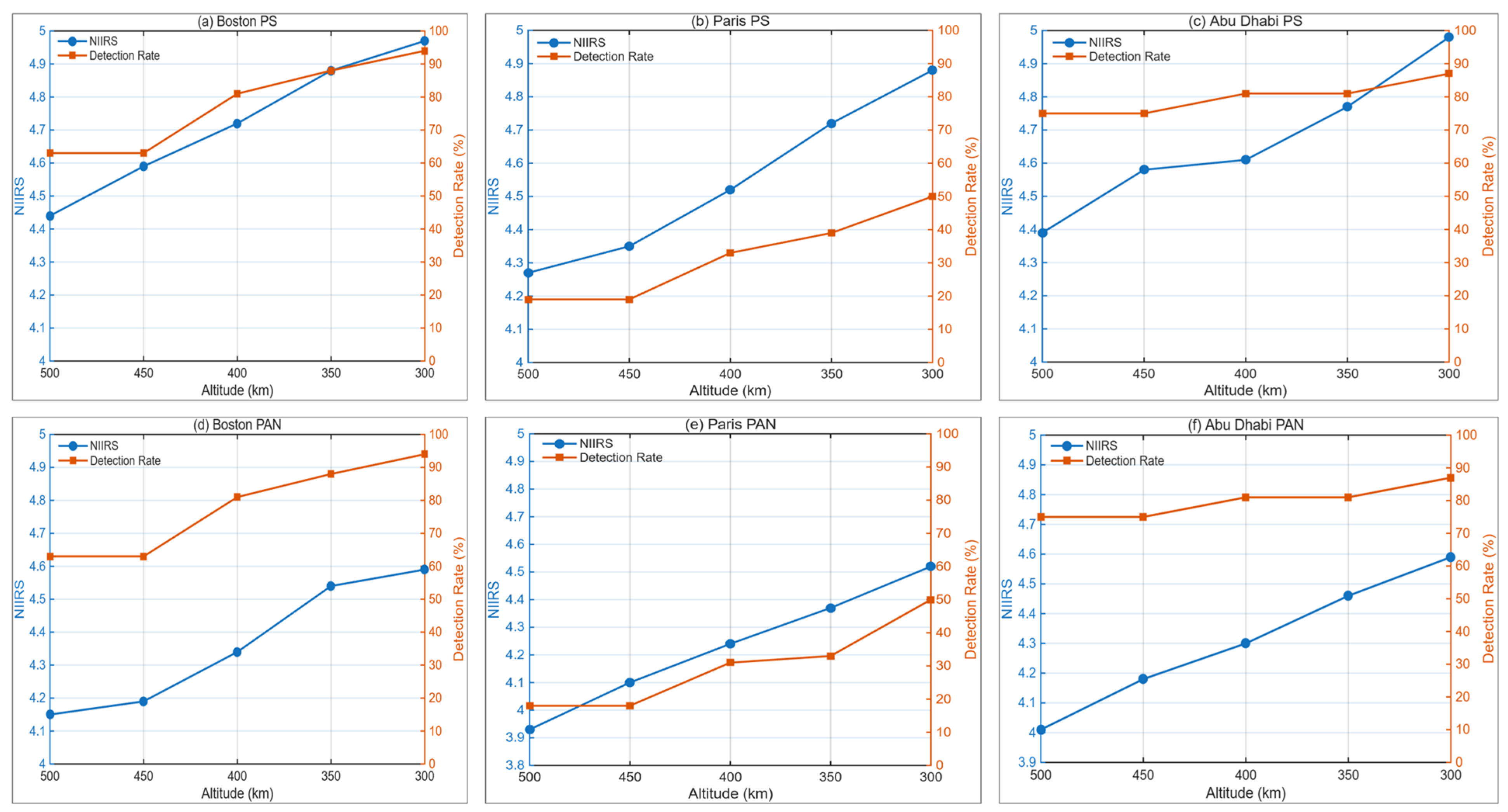
Altitude-dependent trends in GSD, NIIRS, and detection rate for the Boston, Paris, and Abu Dhabi scenes. The altitude-dependent simulation was evaluated for PS and PAN products: (a) Boston PS; (b) Paris PS; (c) Abu Dhabi PS; (d) Boston PAN; (e) Paris PAN; (f) Abu Dhabi PAN. Lower simulated altitude generally produced finer GSD and higher NIIRS, whereas the detection response varied depending on scene content and product type.
Figure 16.
Altitude-dependent trends in GSD, NIIRS, and detection rate for the Boston, Paris, and Abu Dhabi scenes. The altitude-dependent simulation was evaluated for PS and PAN products: (a) Boston PS; (b) Paris PS; (c) Abu Dhabi PS; (d) Boston PAN; (e) Paris PAN; (f) Abu Dhabi PAN. Lower simulated altitude generally produced finer GSD and higher NIIRS, whereas the detection response varied depending on scene content and product type.
Figure 17.
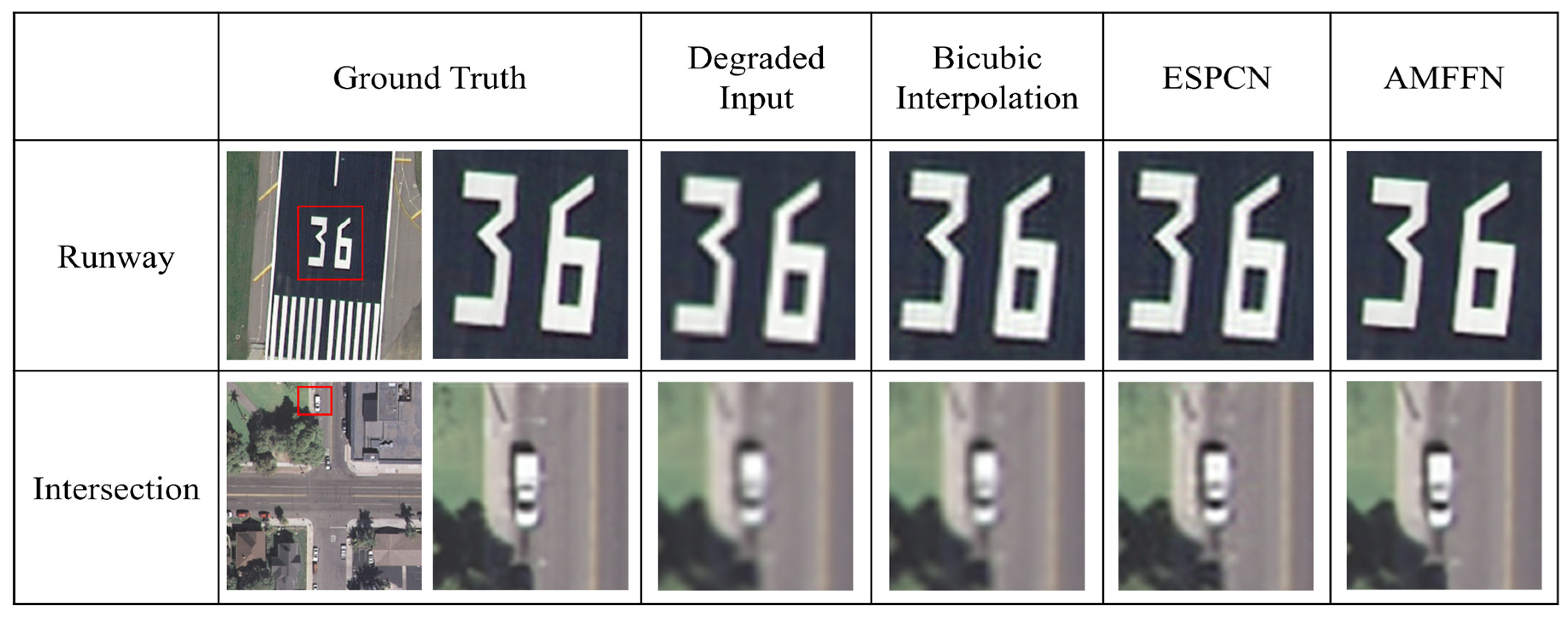
Visual comparison of ×2 SR results on UC Merced Land Use imagery for the runway and intersection examples. The degraded input, bicubic interpolation, ESPCN, and AMFFN are compared with the reference image, and the enlarged views highlight differences in boundary reconstruction.
Figure 17.
Visual comparison of ×2 SR results on UC Merced Land Use imagery for the runway and intersection examples. The degraded input, bicubic interpolation, ESPCN, and AMFFN are compared with the reference image, and the enlarged views highlight differences in boundary reconstruction.
Figure 18.
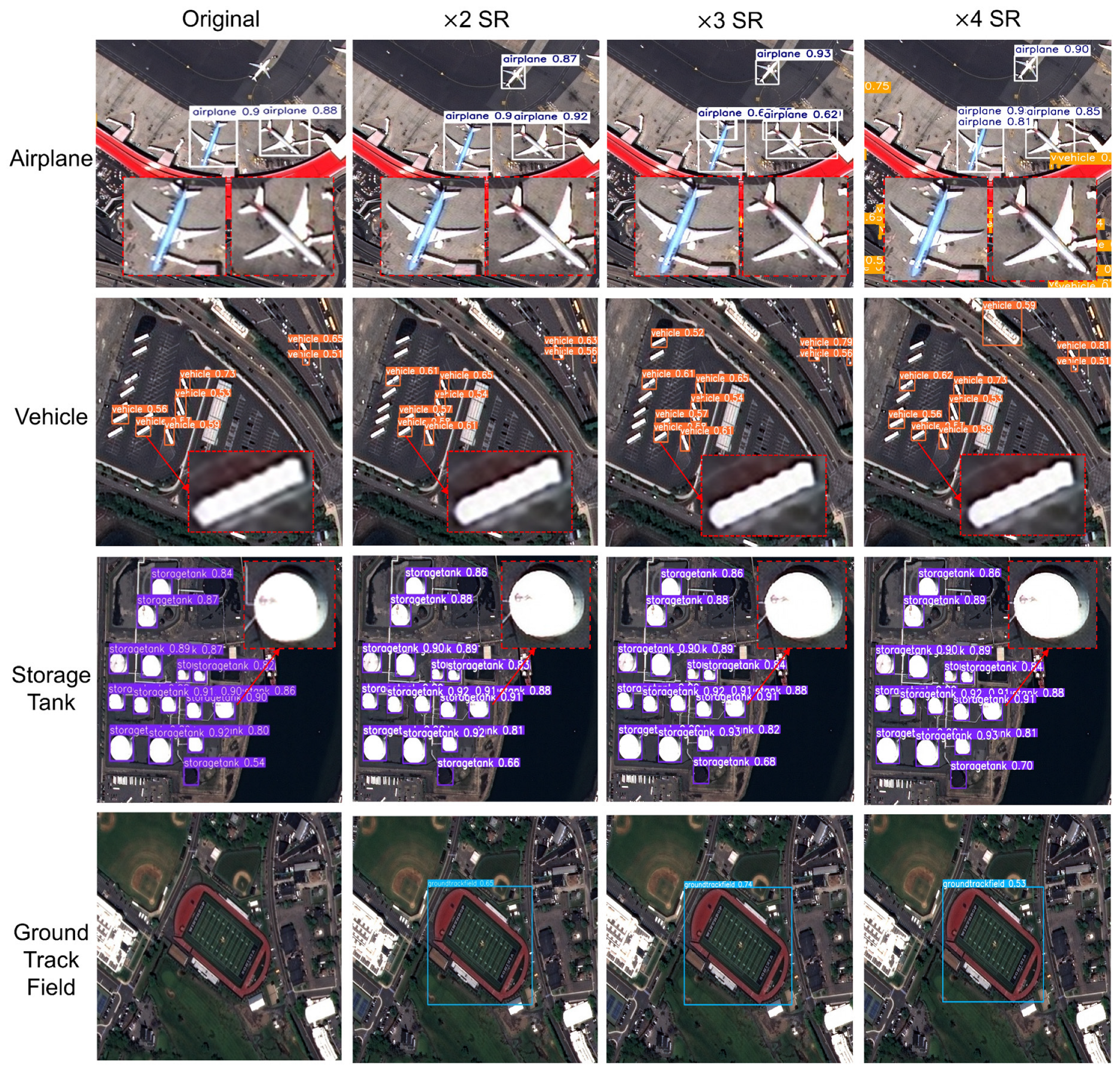
AMFFN-based SR results and object-detection examples for representative NEONSAT-1 PS image chips. The original PS images and SR outputs at ×2, ×3, and ×4 are shown for representative target classes, including airplane, vehicle, storage tank and ground-track field. The examples illustrate target-dependent changes in apparent sharpness, local texture, and object-detection outputs under different SR scaling factors.
Figure 18.
AMFFN-based SR results and object-detection examples for representative NEONSAT-1 PS image chips. The original PS images and SR outputs at ×2, ×3, and ×4 are shown for representative target classes, including airplane, vehicle, storage tank and ground-track field. The examples illustrate target-dependent changes in apparent sharpness, local texture, and object-detection outputs under different SR scaling factors.
Figure 19.
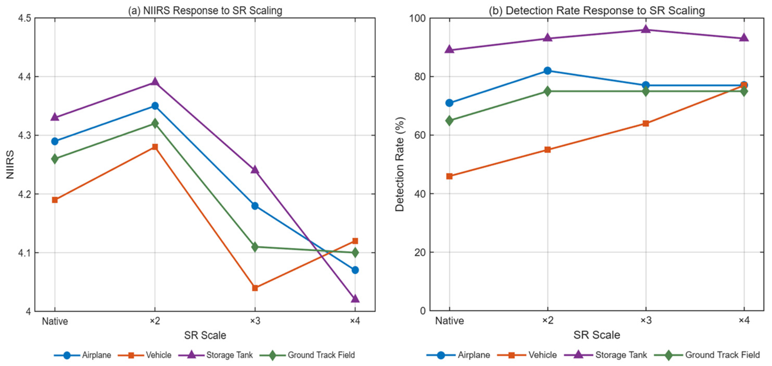
Quantitative responses of NIIRS and detection rate to SR scaling for the NEONSAT-1 SR case study: (a) NIIRS response to the original PS images and AMFFN-based SR outputs at ×2, ×3, and ×4; (b) detection rate response for airplane, vehicle, storage tank, and ground-track field. The results show that SR scaling affects NIIRS and detection rate differently depending on target class, indicating that higher SR scale does not necessarily produce proportional improvement in object detection.
Figure 19.
Quantitative responses of NIIRS and detection rate to SR scaling for the NEONSAT-1 SR case study: (a) NIIRS response to the original PS images and AMFFN-based SR outputs at ×2, ×3, and ×4; (b) detection rate response for airplane, vehicle, storage tank, and ground-track field. The results show that SR scaling affects NIIRS and detection rate differently depending on target class, indicating that higher SR scale does not necessarily produce proportional improvement in object detection.
Table 1.
NEONSAT system specifications.
Table 1.
NEONSAT system specifications.
| Parameters | Value |
|---|
| Orbit | Sun-synchronous |
| Altitude (km) | 500 |
| Weight (kg) | <100 |
| Resolution (m) | PAN: ≤1; MS: ≤4 |
| MTF (%) | PAN: ≥7; MS: ≥20 |
| SNR | PAN and MS: ≥90 |
| Swath (km) | ≥9.76 at nadir |
Table 2.
NEONSAT analysis subsets and auxiliary benchmark datasets used in this study.
Table 2.
NEONSAT analysis subsets and auxiliary benchmark datasets used in this study.
| Section | Data Subset | Date | Product/Target | Purpose |
|---|
| Section 4.1 | Boston | 1 June 2024 | PS, PAN, MS | Product-level comparison of NIIRS and detection rate |
| Section 4.2.1 | Ideal digital edge target | N/A | Synthetic edge pattern | Controlled sensitivity analysis of MTF, RER, and NIIRS |
| Section 4.2.1 | Salon-de-Provence, France | 9 July 2024 | Real NEONSAT edge target | Validation of MTF sensitivity using an observed edge target |
| Section 4.2.1 | Boston | 1 June 2024 | PS | Quantitative comparison of system MTF effects on NIIRS and detection rate |
| Section 4.2.2 | Boston | 1 June 2024 | PS, PAN | Altitude-dependent simulation across representative scenes |
| Paris | 10 August 2024 |
| Abu Dhabi | 14 December 2024 |
| Section 4.3.2 | Selected PS image chips | 1 June 2024 | PS + SR outputs | SR scaling analysis; detection-rate evaluation for four target classes * |
| Section 3.4 | DIOR | N/A | Object-detection benchmark | YOLOv8 training and fine-tuning |
| Section 3.5 and Section 4.3.1 | US Merced Land Use | N/A | Runway and intersection subset | Controlled super-resolution validation |
Table 3.
Surrogate fitting coefficients estimated separately for PAN, PS, and MS products from NEONSAT-1 imagery.
Table 3.
Surrogate fitting coefficients estimated separately for PAN, PS, and MS products from NEONSAT-1 imagery.
| Surrogate Fitting Coefficients |
|---|
| | | | | |
| PAN | 7.17 | −1.29 | 3.11 | 0.06 |
| PS | 7.68 | −1.43 | 3.23 | 0.004 |
| MS | 6.57 | −1.30 | 3.92 | 0.01 |
Table 4.
Detection rates and NIIRS statistics for the PS product.
Table 4.
Detection rates and NIIRS statistics for the PS product.
| | Detection Rate (%) | NIIRS Range | NIIRS Average |
|---|
| Vehicle | 63.00 | 3.73–4.72 | 4.22 |
| Airplane | 57.00 | 4.54–4.93 | 4.82 |
| Storage Tank | 83.00 | 4.00–4.58 | 4.33 |
| Ground-Track Field | 69.00 | 3.93–4.44 | 4.26 |
| Total | 71.00 | 3.73–4.93 | 4.41 |
Table 5.
Detection rates and NIIRS statistics for the PAN product.
Table 5.
Detection rates and NIIRS statistics for the PAN product.
| | Detection Rate (%) | NIIRS Range | NIIRS Average |
|---|
| Vehicle | 58.00 | 3.60–4.61 | 4.13 |
| Airplane | 36.00 | 3.95–4.26 | 4.12 |
| Storage Tank | 90.00 | 3.93–4.34 | 4.13 |
| Ground-Track Field | 12.00 | 3.71–4.48 | 4.10 |
| Total | 65.00 | 3.60–4.61 | 4.12 |
Table 6.
Detection rates and NIIRS statistics for the MS product.
Table 6.
Detection rates and NIIRS statistics for the MS product.
| | Detection Rate (%) | NIIRS Range | NIIRS Average |
|---|
| Vehicle | N/A | N/A | N/A |
| Airplane | 2.00 | 2.54–3.33 | 2.97 |
| Storage Tank | 77.00 | 2.59–3.09 | 2.89 |
| Ground-Track Field | 69.00 | 2.72–3.15 | 2.97 |
| Total | 57.00 | 2.54–3.33 | 2.94 |
Table 7.
Quantitative image-quality metrics for the real NEONSAT edge target under the controlled cases.
Table 7.
Quantitative image-quality metrics for the real NEONSAT edge target under the controlled cases.
| Optic | System | Image Quality | Note |
|---|
| Conic Coefficient () | MTF (%) | MTF (%) | RER | SNR | NIIRS |
|---|
| −1.9450 | 5 | 2.20 | 0.32 | 25.70 | 3.87 | |
| −1.9430 | 11 | 4.69 | 0.34 | 27.12 | 3.96 | |
| −1.9416 | 15 | 6.60 | 0.36 | 27.86 | 4.02 | |
| −1.9406 | 18 | 7.96 | 0.37 | 28.51 | 4.06 | NEONSAT |
| −1.9400 | 20 | 8.74 | 0.38 | 28.85 | 4.08 | |
| −1.9380 | 25 | 10.95 | 0.39 | 29.21 | 4.11 | |
Table 8.
Quantitative image-quality metrics and detection rates for the Boston PS scene under the controlled cases.
Table 8.
Quantitative image-quality metrics and detection rates for the Boston PS scene under the controlled cases.
| Case | (%) | GSD (m) | RER | SNR | NIIRS | Detection Rate (%) | Note |
|---|
| (a) | 2 | 0.939 | 0.305 | 21.56 | 3.58 | 58.2 | |
| (b) | 5 | 0.939 | 0.321 | 21.52 | 3.63 | 59.5 | |
| (c) | 7 | 0.939 | 0.327 | 21.58 | 3.65 | 62.1 | |
| (d) | 8 | 0.939 | 0.332 | 21.68 | 3.67 | 62.1 | NEONSAT |
| (e) | 9 | 0.939 | 0.338 | 21.60 | 3.69 | 64.7 | |
| (f) | 11 | 0.939 | 0.344 | 21.46 | 3.71 | 66.0 | |
Table 9.
Summary of altitude-dependent GSD, NIIRS, and detection rate results for the Boston, Paris, and Abu Dhabi scenes using PS and PAN products.
Table 9.
Summary of altitude-dependent GSD, NIIRS, and detection rate results for the Boston, Paris, and Abu Dhabi scenes using PS and PAN products.
| Study Area | Product Type | Altitude (km) | GSD (m) | Detection Rate (%) | NIIRS Range | NIIRS Average |
|---|
| Boston | PS | 300–500 | 0.49–0.80 | 63–94 | 4.44–4.97 | 4.72 |
| Boston | PAN | 63–88 | 4.15–4.59 | 4.36 |
| Paris | PS | 0.52–0.84 | 19–50 | 4.27–4.88 | 4.54 |
| Paris | PAN | 18–50 | 3.93–4.52 | 4.23 |
| Abu Dhabi | PS | 0.52–0.84 | 75–87 | 4.39–4.98 | 4.66 |
| Abu Dhabi | PAN | 75–87 | 4.01–4.58 | 4.31 |
Table 10.
Quantitative reconstruction accuracy and computational cost of the candidate SR methods on the UC Merced ×2 benchmark.
Table 10.
Quantitative reconstruction accuracy and computational cost of the candidate SR methods on the UC Merced ×2 benchmark.
| | Degraded Input | Bicubic | ESPCN | AMFFN |
|---|
| PSNR | 30.70 | 32.42 | 33.52 | 35.44 |
| SSIM | 0.8610 | 0.8986 | 0.9175 | 0.9378 |
| Parameters * | N/A | N/A | 63,724 | 298,112 |
| FLOPs (G) * | N/A | N/A | 2.10 | 8.76 |
| Time (ms) * | N/A | 0.77 | 4.59 | 36.54 |




 ,
,