Impact Study of Assimilating Fengyun-3 GNSS-R Ocean Surface Winds in the Weather Research and Forecasting Model: Sensitivity Analysis on Observation Error Specifications
 , , , , ,
Highlights
- Optimal assimilation of FY-3E GNSS-R winds in WRF is achieved using a static observation error of 6 m/s without data thinning.
- GNSS-R wind assimilation significantly improves atmospheric analyses, with impacts extending from the surface up to 700 hPa in a sensitivity experiment and higher levels in cycling OSEs.
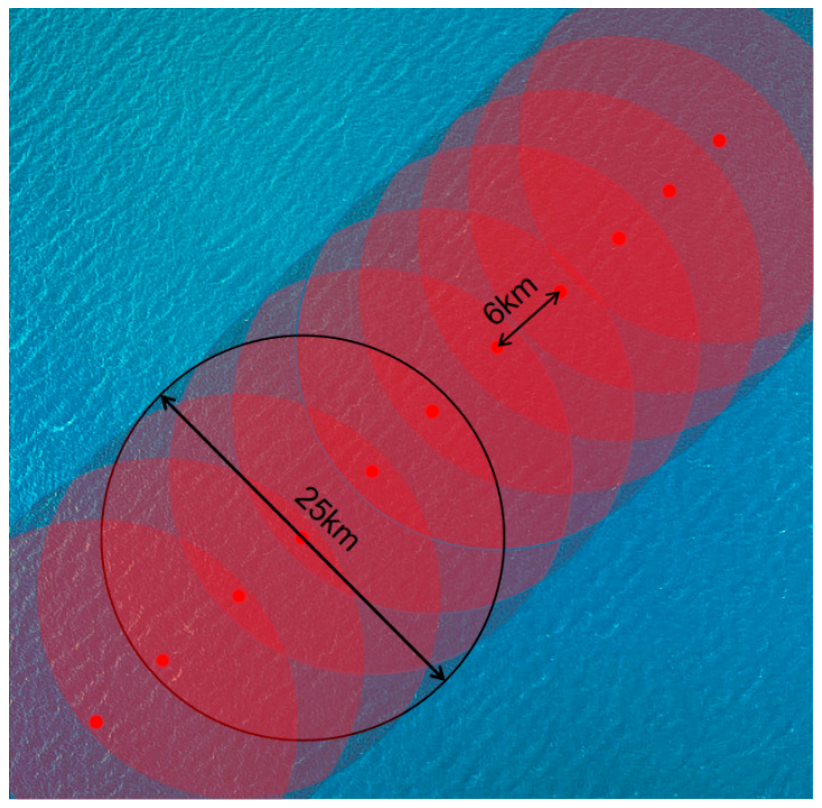
- The dense along-track sampling of GNSS-R observations requires careful observation error specification, which plays a critical role in data assimilation.
- The observation error configuration and OSEs provide a practical reference for assimilating GNSS-R winds in WRF, and can be extended to other NWP systems.
Abstract
1. Introduction
2. WRF Model and Data
2.1. WRF Forecast and Data Assimilation Systems
2.2. FY-3E GNSS-R Ocean Surface Wind Observations
2.3. Validation Datasets: ECMWF ERA5 and HSCAT Wind Data
3. A Case Study of Assimilating GNSS-R Wind Speed
3.1. Experiment Description
3.2. Results
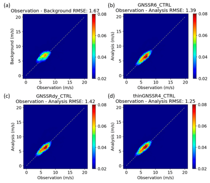
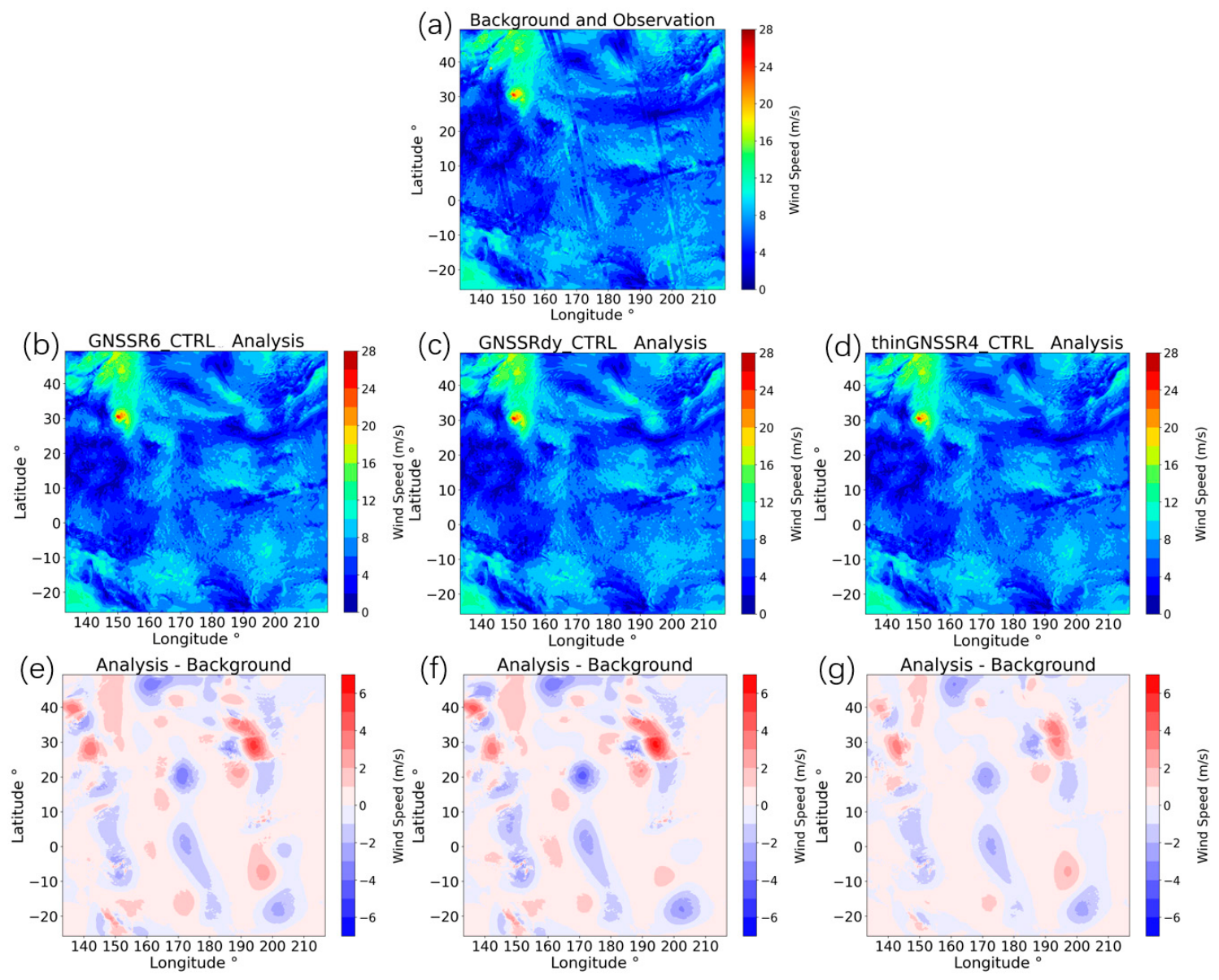
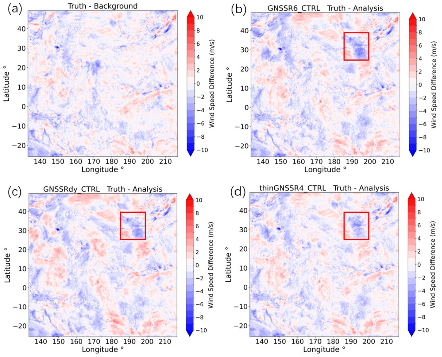
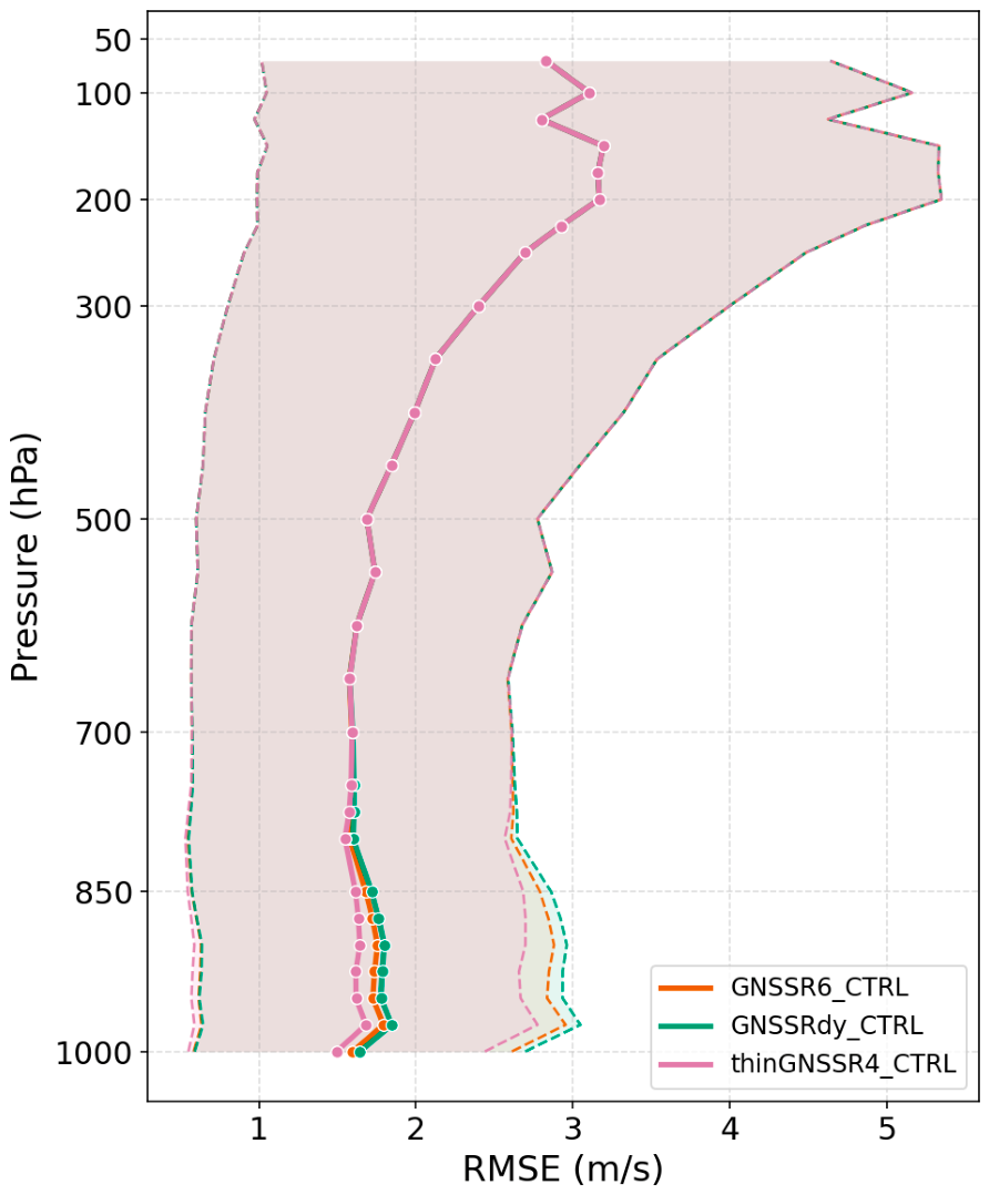
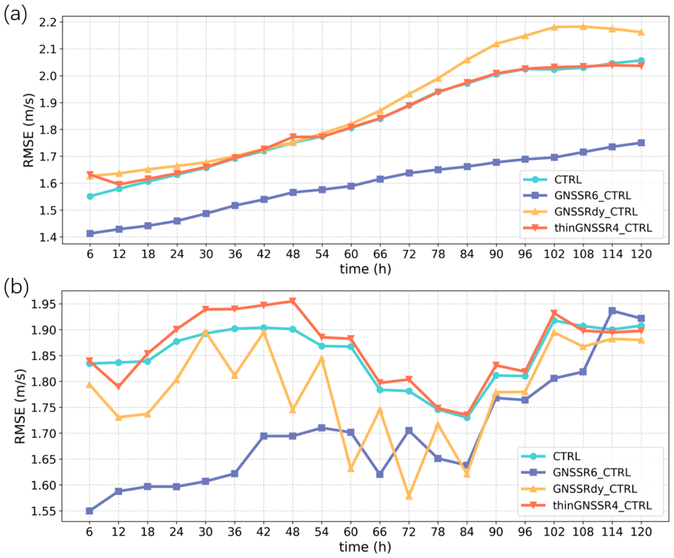
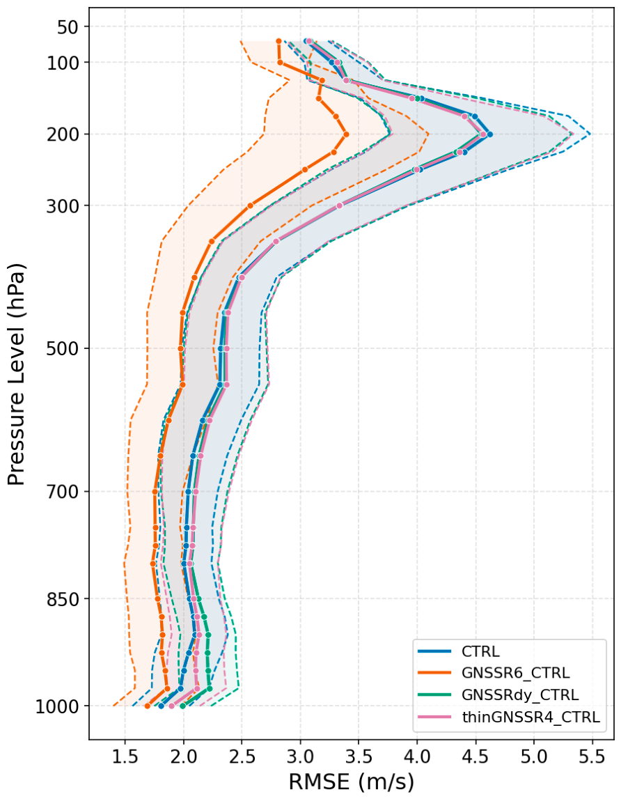
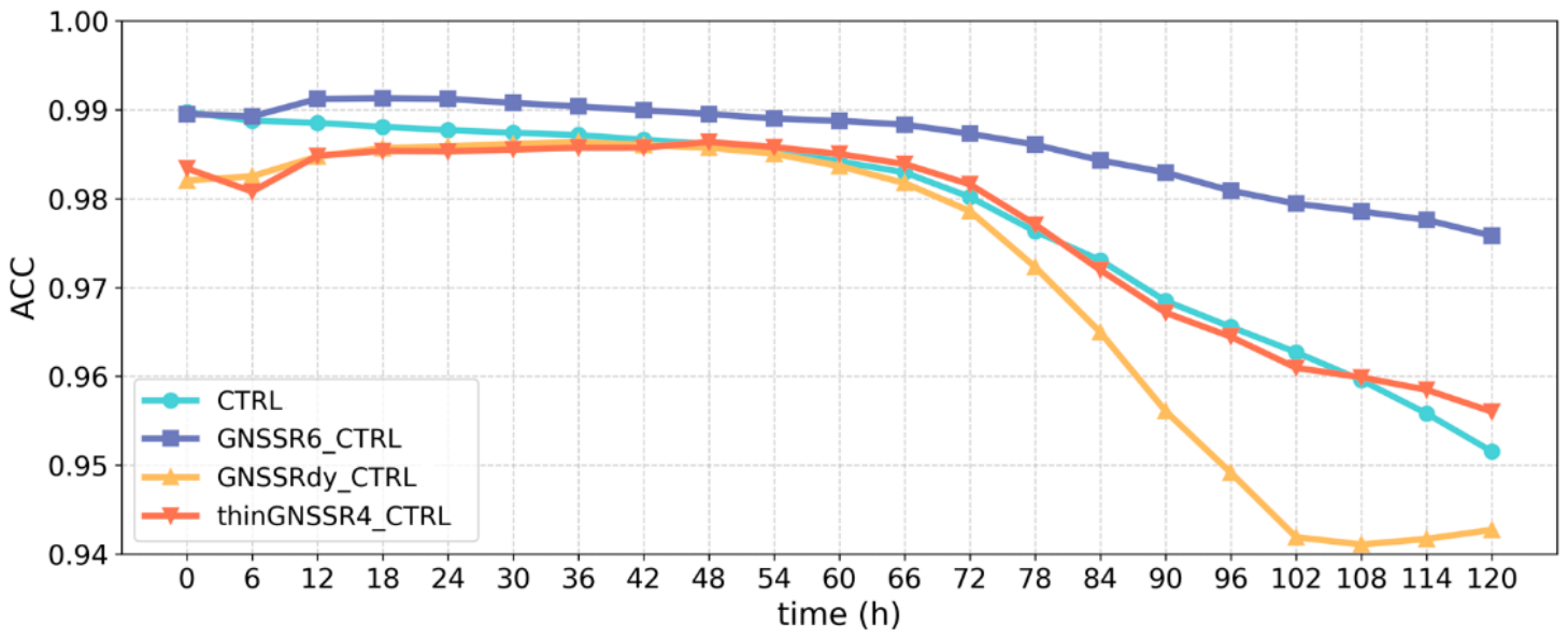
- GNSSR6_CTRL: GNSS-R wind speeds are assimilated with a static observation error of 6 m/s.
- GNSSRdy_CTRL: GNSS-R wind speeds are assimilated with dynamic observation errors inflated by a factor of 4.
- thinGNSSR4_CTRL: GNSS-R wind speeds are assimilated with a static observation error of 4 m/s and data thinning applied.
4. Observing System Experiments
4.1. Experiment Description
4.2. Results
5. Discussion
6. Conclusions
Author Contributions
Funding
Data Availability Statement
Conflicts of Interest
References
- Tollinger, M.; Graversen, R.G. Validation of a SAR-Only Wind-Vector Retrieval Against Shipborne In Situ Wind Observations in the European Arctic. IEEE Trans. Geosci. Remote Sens. 2024, 62, 1–11. [Google Scholar] [CrossRef] [Scilit]
- Fang, H.; Perrie, W.; Fan, G.; Li, Z.; Cai, J.; He, Y.; Yang, J.; Xie, T.; Zhu, X. High-resolution sea surface wind speeds of Super Typhoon Lekima (2019) retrieved by Gaofen-3 SAR. Front. Earth Sci. 2022, 16, 90–98. [Google Scholar] [CrossRef] [Scilit]
- Xu, X.G.; Dong, X.L.; Zhu, D.; Lang, S.Y. High Winds from Combined Active and Passive Measurements of HY-2A Satellite. IEEE J. Sel. Top. Appl. Earth Obs. Remote Sens. 2018, 11, 4339–4348. [Google Scholar] [CrossRef] [Scilit]
- Li, X.Y.; Zuo, X.H.; Wang, J. SSS Retrieval Using C- and X-Band Microwave Radiometer Observations in Coastal Oceans. Atmosphere 2026, 17, 250. [Google Scholar] [CrossRef] [Scilit]
- Wu, M.M.; Wang, H.; Wan, L.Y.; Wang, J.J.; Wang, Y.; Wang, J.K. The Impacts of the Application of the Ensemble Optimal Interpolation Method in Global Ocean Wave Data Assimilation. Atmosphere 2023, 14, 818. [Google Scholar] [CrossRef] [Scilit]
- Sebastianelli, S.; D’Adderio, L.P.; Sanò, P.; Casella, D.; Panegrossi, G. Near-surface wind field characterization of medicanes using satellite observations. Atmos. Res. 2026, 334, 108734. [Google Scholar] [CrossRef] [Scilit]
- Zhu, Y.C.; Lu, Q.L.; Ge, M.R.; Qu, X.C.; Tao, T.Y.; Yu, K.G.; Li, S.P. Attention enhanced ResNet for ocean surface wind speed retrieval using CYGNSS observables. Adv. Space Res. 2026, 77, 2906–2921. [Google Scholar] [CrossRef] [Scilit]
- Li, Z.; Guo, F.; Zhang, X.H.; Zhang, Z.Y.; Zhu, Y.F.; Yang, W.T.; Chen, P.; Wu, Z.H. Spaceborne Global Navigation Satellite System-Reflectometry sea surface wind speed retrieval based on machine learning and spatiotemporal filtering. J. Appl. Remote Sens. 2025, 19, 044507. [Google Scholar] [CrossRef] [Scilit]
- Zhang, Z.; Xu, J.; Jing, G.; Yang, D.; Zhang, Y. Physics-Informed Transformer Networks for Interpretable GNSS-R Wind Speed Retrieval. Remote Sens. 2025, 17, 3805. [Google Scholar] [CrossRef] [Scilit]
- Qiao, X.; Huang, W. Ocean Surface Wind Speed Estimation from GNSS-R Data Using Physics-Informed Attention-Aided Convolutional Neural Network. IEEE Trans. Geosci. Remote Sens. 2025, 63, 1–16. [Google Scholar] [CrossRef] [Scilit]
- Du, H.; Li, W.; Cardellach, E.; Ribó, S.; Rius, A.; Nan, Y. Deep residual fully connected network for GNSS-R wind speed retrieval and its interpretation. Remote Sens. Environ. 2024, 313, 114375. [Google Scholar] [CrossRef] [Scilit]
- Katzberg, S.J.; Torres, O.; Ganoe, G. Calibration of reflected GPS for tropical storm wind speed retrievals. Geophys. Res. Lett. 2006, 33, L18602. [Google Scholar] [CrossRef] [Scilit]
- Balasubramaniam, R.; Ruf, C. Characterization of rain impact on L-Band GNSS-R ocean surface measurements. Remote Sens. Environ. 2020, 239, 111607. [Google Scholar] [CrossRef] [Scilit]
- Ruf, C.S.; Atlas, R.; Chang, P.S.; Clarizia, M.P.; Garrison, J.L.; Gleason, S.; Katzberg, S.J.; Jelenak, Z.; Johnson, J.T.; Majumdar, S.J.; et al. New Ocean Winds Satellite Mission to Probe Hurricanes and Tropical Convection. Bull. Am. Meteorol. Soc. 2016, 97, 385–395. [Google Scholar] [CrossRef] [Scilit]
- Jales, P.; Cartwright, J.; Talpe, M.; Mashburn, J.; Yuasa, T.; Nogues-Correig, O.; Nguyen, V.; Freeman, V. Spire Global’s Operational GNSS-Reflectometry Constellation for Earth Surface Observations. In Proceedings of the IGARSS 2023—2023 IEEE International Geoscience and Remote Sensing Symposium, Pasadena, CA, USA, 16–21 July 2023. [Google Scholar]
- Jing, C.; Niu, X.; Duan, C.; Lu, F.; Di, G.; Yang, X. Sea Surface Wind Speed Retrieval from the First Chinese GNSS-R Mission: Technique and Preliminary Results. Remote Sens. 2019, 11, 3013. [Google Scholar] [CrossRef] [Scilit]
- Huang, F.; Sun, Y.; Xia, J.; Yin, C.; Bai, W.; Du, Q.; Zhai, X.; Yang, G.; Chen, L.; Lu, W.; et al. Progress on the GNSS-R Product from Fengyun-3 Missions. In Proceedings of the IGARSS 2024—2024 IEEE International Geoscience and Remote Sensing Symposium, Athens, Greece, 7–12 July 2024. [Google Scholar]
- Huang, F.; Yin, C.; Liu, Y.; Sun, Y.; Xia, J.; Bai, W.; Tang, Q.; Wang, X.; Du, Q.; Cai, Y.; et al. Tianmu-1 Constellation GNSS-R In-Orbit Performance: Spatiotemporal Characteristics, Product Applications, and Polarimetric Features. IEEE Trans. Geosci. Remote Sens. 2025, 63, 1–20. [Google Scholar] [CrossRef] [Scilit]
- Yang, S.; Zou, X. Assimilating Tianmu-1 RO Data from a 23-Satellite Constellation to Enhance the Track Forecasts of Typhoon Gaemi (2024). Geophys. Res. Lett. 2025, 52, e2025GL115679. [Google Scholar] [CrossRef] [Scilit]
- Ray, S.; Moharana, S.S.; Nag, A.; Swain, D. Evaluation of Oceansat-3 gridded wind accuracy for low to extreme wind speed conditions. Int. J. Remote Sens. 2025, 46, 6403–6427. [Google Scholar] [CrossRef] [Scilit]
- Powell, C.E.; Ruf, C.S. A Method for Estimating and Partitioning the Covariance of Wind Speed Observation Error from GNSS Reflectometry. J. Atmos. Ocean. Technol. 2025, 42, 1027–1040. [Google Scholar] [CrossRef] [Scilit]
- Hoffman, R.N. The Effect of Thinning and Superobservations in a Simple One-Dimensional Data Analysis with Mischaracterized Error. Mon. Weather Rev. 2018, 146, 1181–1195. [Google Scholar] [CrossRef] [Scilit]
- Majumdar, S.J.; Atlas, R.; Hoffman, R.; Leidner, S.M.; McNoldy, B.; Annane, B. A Study of the HWRF Analysis and Forecast Impact of Realistically Simulated CYGNSS Observations Assimilated as Scalar Wind Speeds and as VAM Wind Vectors. Mon. Weather Rev. 2018, 146, 2221–2236. [Google Scholar]
- McNoldy, B.; Annane, B.; Majumdar, S.; Delgado, J.; Bucci, L.; Atlas, R. Impact of Assimilating CYGNSS Data on Tropical Cyclone Analyses and Forecasts in a Regional OSSE Framework. Mar. Technol. Soc. J. 2017, 51, 7–15. [Google Scholar] [CrossRef] [Scilit]
- Zhang, S.; Pu, Z.; Posselt, D.J.; Atlas, R. Impact of CYGNSS Ocean Surface Wind Speeds on Numerical Simulations of a Hurricane in Observing System Simulation Experiments. J. Atmos. Ocean. Technol. 2017, 34, 375–383. [Google Scholar] [CrossRef] [Scilit]
- Lin, K.-J.; Yang, S.-C.; Chen, S.S. Improving Analysis and Prediction of Tropical Cyclones by Assimilating Radar and GNSS-R Wind Observations: Ensemble Data Assimilation and Observing System Simulation Experiments Using a Coupled Atmosphere–Ocean Model. Weather Forecast. 2022, 37, 1533–1552. [Google Scholar] [CrossRef] [Scilit]
- Leidner, S.M.; Annane, B.; McNoldy, B.; Hoffman, R.; Atlas, R. Variational Analysis of Simulated Ocean Surface Winds from the Cyclone Global Navigation Satellite System (CYGNSS) and Evaluation Using a Regional OSSE. J. Atmos. Ocean. Technol. 2018, 35, 1571–1584. [Google Scholar] [CrossRef] [Scilit]
- Cui, Z.; Pu, Z.; Tallapragada, V.; Atlas, R.; Ruf, C.S. A Preliminary Impact Study of CYGNSS Ocean Surface Wind Speeds on Numerical Simulations of Hurricanes. Geophys. Res. Lett. 2019, 46, 2984–2992. [Google Scholar] [CrossRef] [Scilit]
- Li, X.; Mecikalski, J.R.; Lang, T.J. A Study on Assimilation of CYGNSS Wind Speed Data for Tropical Convection during 2018 January MJO. Remote Sens. 2020, 12, 1243. [Google Scholar] [CrossRef] [Scilit]
- Mueller, M.J.; Annane, B.; Leidner, S.M.; Cucurull, L. Impact of CYGNSS-Derived Winds on Tropical Cyclone Forecasts in a Global and Regional Model. Mon. Weather Rev. 2021, 149, 3433–3447. [Google Scholar] [CrossRef] [Scilit]
- Pu, Z.; Wang, Y.; Li, X.; Ruf, C.; Bi, L.; Mehra, A. Impacts of Assimilating CYGNSS Satellite Ocean-Surface Wind on Prediction of Landfalling Hurricanes with the HWRF Model. Remote Sens. 2022, 14, 2118. [Google Scholar]
- Huang, F.; Xia, J.; Yin, C.; Zhai, X.; Xu, N.; Yang, G.; Bai, W.; Sun, Y.; Du, Q.; Liao, M.; et al. Assessment of FY-3E GNOS-II GNSS-R Global Wind Product. IEEE J. Sel. Top. Appl. Earth Obs. Remote Sens. 2022, 15, 7899–7912. [Google Scholar] [CrossRef] [Scilit]
- Liu, S.; Lin, W.; Portabella, M.; Wang, Z. Characterization of Tropical Cyclone Intensity Using the HY-2B Scatterometer Wind Data. Remote Sens. 2022, 14, 1035. [Google Scholar] [CrossRef] [Scilit]
- Yu, Y.; Zhang, W.; Wu, Z.; Yang, X.; Cao, X.; Zhu, M. Assimilation of HY-2A scatterometer sea surface wind data in a 3DVAR data assimilation system—A case study of Typhoon Bolaven. Front. Earth Sci. 2015, 9, 192–201. [Google Scholar] [CrossRef] [Scilit]



| Reference | Observation Type | Model and System | Strategy of Observation Error Settings |
|---|---|---|---|
| Majumdar and Atlas [23] | Simulated | WRF & GSI | Simulated errors with typical values of 2–4 m/s. |
| McNoldy and Annane [24] | Simulated | HWRF & GSI | Errors inversely proportional to antenna gain. |
| Zhang and Pu [25] | Simulated | HWRF & GSI | Thinned to 27 km, errors were estimated by comparing CYGNSS winds with the hurricane NR. |
| Lin and Yang [26] | Simulated | UWIN-CM & WRF-LETKF | 2 m/s (<20 m/s) and 10% (>20 m/s). |
| Leidner and Annane [27] | Simulated | HWRF & GSI | Simulated errors with typical values of 2–4 m/s. |
| Cui and Pu [28] | Real | HWRF & GSI | Thinned at 25 km. The observation error was set to 2.1429 m/s. |
| Li and Mecikalski [29] | Real | WRF & WRFDA | Thinned to 25 km; 2 m/s (<20 m/s) and 10% (>20 m/s). |
| Mueller and Annane [30] | Real | HWRF & GSI | Inflating observation errors by a factor of 5. |
| Pu and Wang [31] | Real | HWRF & GSI | Observations thinned to 25 km; 2 m/s for CYGNSS V2.1 data and 3 m/s for V3.0 data. |
Disclaimer/Publisher’s Note: The statements, opinions and data contained in all publications are solely those of the individual author(s) and contributor(s) and not of MDPI and/or the editor(s). MDPI and/or the editor(s) disclaim responsibility for any injury to people or property resulting from any ideas, methods, instructions or products referred to in the content. |
© 2026 by the authors. Licensee MDPI, Basel, Switzerland. This article is an open access article distributed under the terms and conditions of the Creative Commons Attribution (CC BY) license.
Share and Cite
Wang, G.; Bai, W.; Huang, F.; Sun, Y.; Xia, J.; Wang, X.; Meng, X.; Hu, P.; Yin, C.; Tan, G.; et al. Impact Study of Assimilating Fengyun-3 GNSS-R Ocean Surface Winds in the Weather Research and Forecasting Model: Sensitivity Analysis on Observation Error Specifications. Remote Sens. 2026, 18, 1892. https://doi.org/10.3390/rs18121892
Wang G, Bai W, Huang F, Sun Y, Xia J, Wang X, Meng X, Hu P, Yin C, Tan G, et al. Impact Study of Assimilating Fengyun-3 GNSS-R Ocean Surface Winds in the Weather Research and Forecasting Model: Sensitivity Analysis on Observation Error Specifications. Remote Sensing. 2026; 18(12):1892. https://doi.org/10.3390/rs18121892
Chicago/Turabian StyleWang, Guanyi, Weihua Bai, Feixiong Huang, Yueqiang Sun, Junming Xia, Xianyi Wang, Xiangguang Meng, Peng Hu, Cong Yin, Guangyuan Tan, and et al. 2026. "Impact Study of Assimilating Fengyun-3 GNSS-R Ocean Surface Winds in the Weather Research and Forecasting Model: Sensitivity Analysis on Observation Error Specifications" Remote Sensing 18, no. 12: 1892. https://doi.org/10.3390/rs18121892
APA StyleWang, G., Bai, W., Huang, F., Sun, Y., Xia, J., Wang, X., Meng, X., Hu, P., Yin, C., Tan, G., Wu, R., Du, Y., & Meng, X. (2026). Impact Study of Assimilating Fengyun-3 GNSS-R Ocean Surface Winds in the Weather Research and Forecasting Model: Sensitivity Analysis on Observation Error Specifications. Remote Sensing, 18(12), 1892. https://doi.org/10.3390/rs18121892