Adaptive Unsupervised Detection of Field-Scale Irrigation from High-Resolution SAR Soil Moisture Maps

Highlights

What are the main findings?

• High-resolution ($~100$ m) SSM maps derived from Sentinel-1 and -2 timeseries enable early-season, field-scale irrigation detection.
• Detection accuracy is driven by Sentinel-1 timing, crop growth stage, and the interval between irrigation and SAR overpass.

What are the implications of the main findings?

• Strong correlation between soil moisture and irrigation depth shows the potential to support the retrieval of applied water volumes.
• Synergy between C-band and L-band SAR can improve irrigation monitoring throughout the full crop cycle.

Abstract

The purpose of this work is to investigate the use of high-resolution ($~100$ m) surface soil moisture (SSM) maps derived from Sentinel-1 (S-1) and Sentinel-2 (S-2) data to identify irrigation events occurring in the Riaza irrigation district (Castilla y León region, Spain) from 2017 to 2021. The proposed method is based on the application of the Constant False Alarm Rate (CFAR) algorithm, which is an adaptive and unsupervised thresholding algorithm traditionally used for target detection in SAR images. This algorithm uses a sliding window approach that allows an adaptive threshold estimate for each pixel of the image, depending on the distribution of the surrounding pixels. The analysis was carried out on fields cultivated with maize, sugar beet and sunflower. Results show that the Overall Accuracy (OA) of the detection mainly depends on the time span (TS) between the S-1 passage and the irrigation event, the acquisition timing and the development stage of the vegetation. Indeed, the OA reaches a mean of $78\%$ and $70\%$, respectively, for the $6$ a.m. and $6$ p.m. acquisitions, when the irrigation events occur within $36$ h before the S-1 passage, and it follows a downward trend as the TS increases. On the other hand, when the vegetation reaches the mature stage, the mean OA decreases respectively to $56\%$ and $52\%$. Stemming from the event detection, the study explored the estimation of the total irrigated area in the early growing season, showing promising agreement with in situ data, as evidenced by the low Relative Error ($E_r\approx 5.6\%$). Additionally, the analysis revealed a significant correlation between field-scale mean SSM and irrigation depths ($R=0.89$).

1. Introduction

Intensive irrigation, which accounts for more than $90\%$ of global consumptive water use [1], plays a central role in agricultural productivity but can significantly disrupt the terrestrial water cycle, contribute to aquifer depletion, and intensify competition for water resources, particularly in regions already experiencing water stress [2]. Despite its critical importance, a comprehensive understanding of the positive and negative feedbacks of irrigation across the various components and processes of the Earth system remains limited and is increasingly recognized as a scientific priority [3]. A key input for advancing such understanding is the accurate quantification of the spatial extent of irrigated areas and their temporal dynamics [4], which require observations at sufficiently high spatial and temporal resolutions [5]. Current efforts to characterize irrigation rely on a combination of data sources, including census-based surveys [6], national and international statistics (e.g., [7]), and Earth observation (EO) techniques [8]. Each of these approaches presents specific advantages and limitations, making the characterization of their potential and associated uncertainties a timely and relevant research objective [9]. Recent review studies have summarized the state of the art in the use of optical and microwave EO data to retrieve a wide range of irrigation-related variables, including the spatial extent of irrigated areas, the timing of irrigation events, the amount of applied water, and vegetation or crop condition indicators such as the Normalized Difference Vegetation Index (NDVI) [10,11,12,13]. These studies demonstrate the capability of EO data to support large-scale irrigation monitoring across a broad range of spatial and temporal resolutions.

Within this growing body of research, increasing attention has been devoted to approaches based on surface soil moisture (SSM) retrieved from satellite Synthetic Aperture Radar (SAR) systems. SAR-derived SSM products are particularly attractive for irrigation monitoring due to their high resolution ($0.1–1.0$ km). These products are largely unaffected by cloud cover and varying light conditions, allowing for consistent observations in all-weather scenarios. Additionally, they can detect irrigation during the early stages of crop growth [14].

Several studies have leveraged Sentinel-1 (S-1) data for irrigation detection, often in combination with Sentinel-2 (S-2) optical observations. Bazzi et al. (2020) [15] adopted the IDM (Irrigation Detection Model) [16], which uses a change detection approach on backscatter at different spatial scales (field and $10$ km scales) to discern changes linked to irrigation from those caused by rainfalls, achieving an irrigation detection F-score of $76.4\%$. Similar results were obtained by Zappa et al. (2021) [17] by leveraging the spatial and temporal dynamics of SSM at $~500$ m resolution. Le Page et al. (2020) [18] combined an S-1 SSM product and a water balance model to estimate the irrigation event timing, reaching an F-score of $~80\%$. Other works adopted machine learning (ML) models, such as the k-means clustering [19,20], Support Vector Machine, decision trees and Random Forest [21,22] reporting a mean Overall Accuracy of approximately $77\%$.

A parallel line of research has focused on using satellite-derived SSM products and land surface models to quantify daily or monthly irrigation volumes [23,24], produce digital water budget replicas at the basin scale [25] and assess future irrigation requirements under climate change scenarios [26]. Corbari et al. (2025) [23] integrated a combined SMAP-Sentinel-1 soil moisture product into an energy water balance model, demonstrating that both spatial and temporal resolutions are crucial for improving irrigation estimates. Similarly, Dari et al. (2020) [24] explored irrigation volume estimation using the SM2RAIN algorithm applied to $1$ km downscaled SMAP and SMOS data, obtaining good agreement with in situ observations (correlation ranging from $0.58$ to $0.81$, depending on the site).

Building on these recent developments, this study aims to advance current irrigation monitoring approaches by assessing the potential of high-resolution ($~100$ m) SSM maps for the detection of irrigation at the field scale. The high-resolution SSM time series are derived from combined S-1 and S-2 time series through the SMOSAR (version 2) (“Soil MOisture retrieval from multi-temporal SAR data”) software [27]. The methodology proposed for the detection of irrigation leverages a pixel-wise classification framework based on the Constant False Alarm Rate (CFAR) algorithm. By exploiting a sliding-window strategy, CFAR enables the estimation of an adaptive, locally defined classification threshold for each pixel. Subsequently, pixels classified as irrigated or non-irrigated are aggregated at the field scale using parcel boundary information. The methodology is applied to the Riaza irrigation district in the Castilla y León region of Spain, for which detailed records of irrigation scheduling and crop types are available for the 2017–2021 period from the Instituto Tecnológico Agrario de Castilla y León (ITACyL). These data provide a robust reference for the validation and assessment of the proposed approach, enabling a detailed analysis of key factors affecting the Overall Accuracy, including the time span (TS) between the acquisition and the irrigation event, the acquisition timing, and the crop phenological stage influence on irrigation detection performance.

The manuscript is structured into five main sections. Following this introduction, Section 2 describes the in situ and satellite-derived datasets, as well as the proposed methodology, while Section 3 presents the results of the analysis, which are subsequently discussed in Section 4. Lastly, Section 5 provides the concluding remarks.

2. Materials and Methods

2.1. Test Site and In Situ Data

The study area for this investigation is the Riaza irrigation district, located in the Castilla y León region of Spain. A comprehensive database is available for the district, which includes detailed information on crop types and their respective field proportions, field boundaries, irrigation schedules (start and end times for each irrigation event), water consumption, as well as precipitation records from 2017 to 2021. 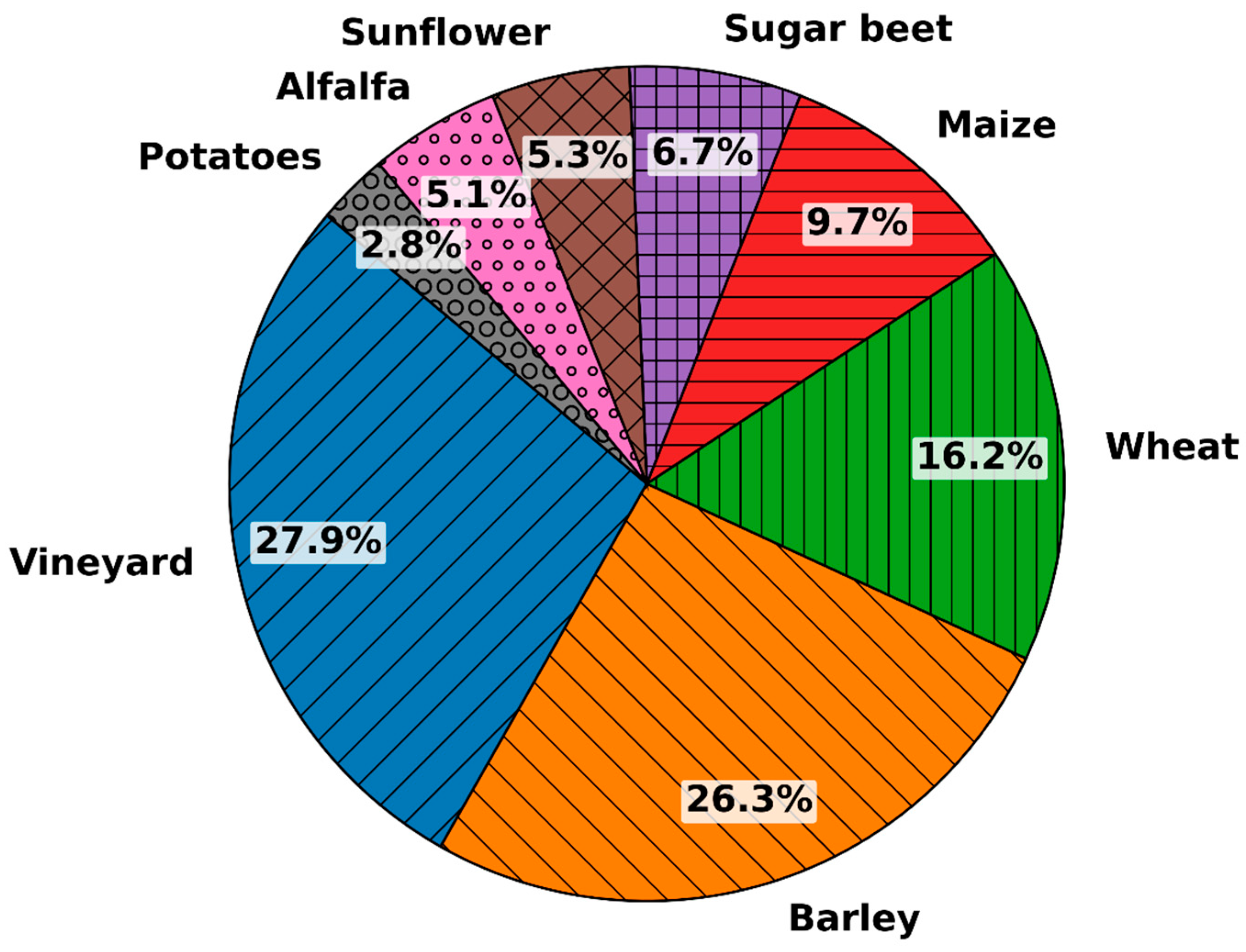The agricultural area covers $5232$ ha and includes $991$ cultivated fields. The chart in Figure 1 describes the percentage of fields occupied by the most widespread crops in the study area, considering only fields with an extent greater than $1$ ha and covered by a homogenous crop for at least $50\%$ of their area. Other than vineyards, the main cultivated crops are barley, wheat and maize ($26.3\%$, $16.2\%$ and $9.7\%$ respectively), followed by alfalfa, sugar beet and sunflower, which represent $17.1\%$ of the total.

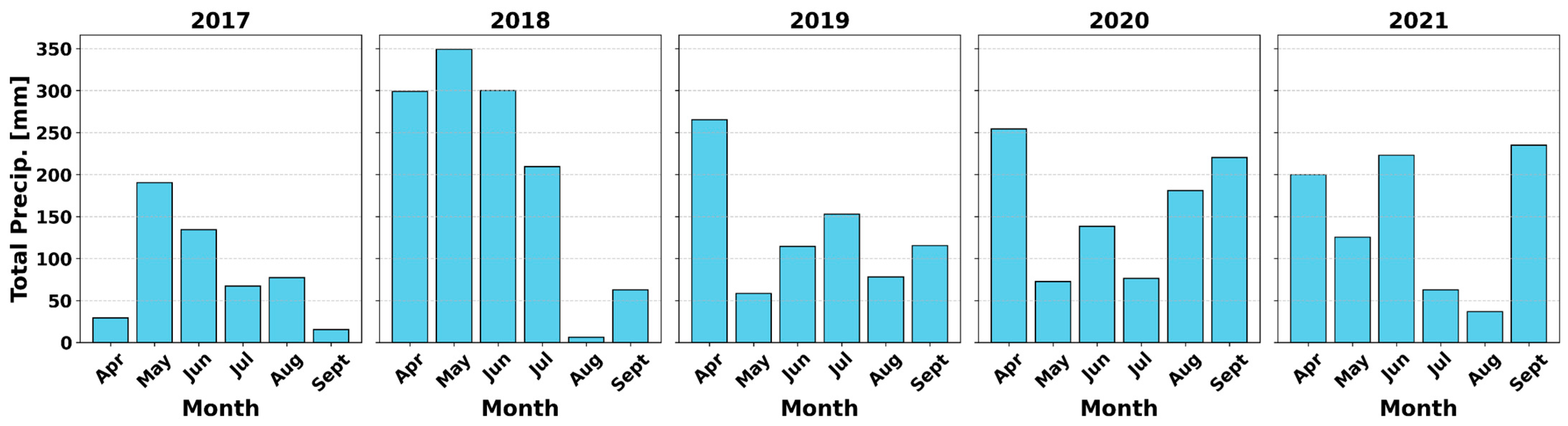
Figure 2 shows the monthly cumulative precipitation from April to September for each year in which irrigation data were available (i.e., 2017–2021). In the analysis SSM maps generated when the meteorological station recorded rainfall were excluded. This is because the occurrence of precipitation significantly obscures the signal of irrigation events, making it difficult to accurately discriminate between irrigated and non-irrigated areas. This concept is further explored in Section 2.5. The study area, as visible from Figure 2, during 2018 was characterized by frequent and heavy precipitation, which caused the exclusion of $60\%$ of this year’s SSM maps from the analysis and the reduction of the total number of useful irrigation events to a negligible number (i.e., $53$); consequently, this year was disregarded during the analysis.

The district’s irrigation is managed through fully automated sprinkler systems. This automation ensures a complete record for each irrigation event, capturing start/end timestamps, durations, and applied water volumes.

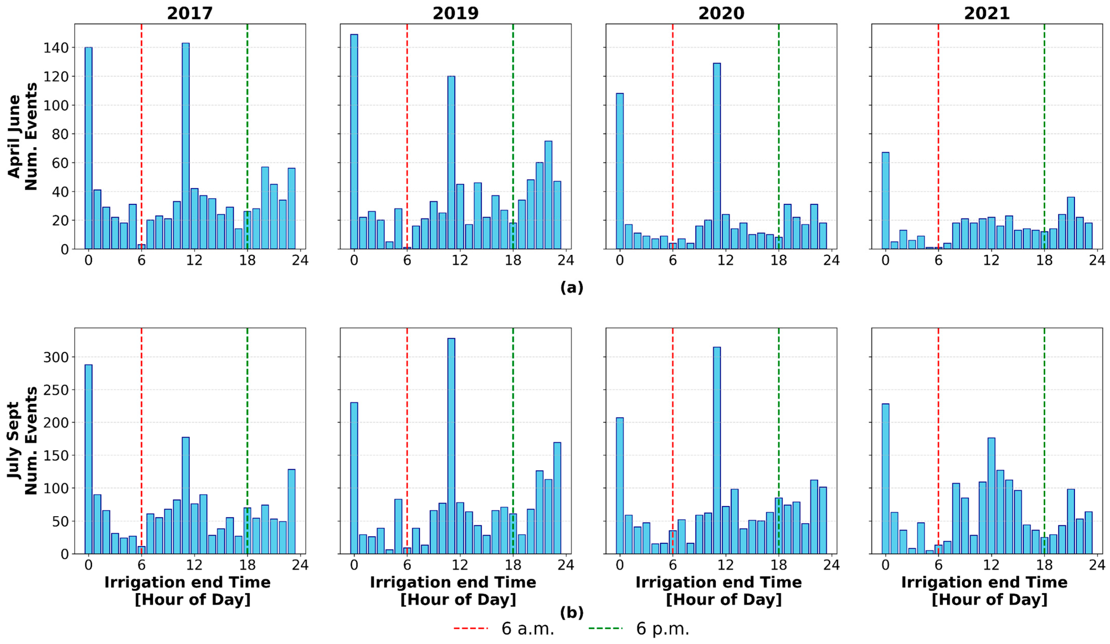
In Figure 3 are depicted the frequency distribution of the ending times of the irrigation events that occurred for summer crops in the April–June (a) and the July–September (b) periods. The data reveal that, except for 2021, the peaks of the ending time are registered around 11:00 and 00:00.

2.2. Sentinel-1 and Sentinel-2 Data

The satellite derived dataset consists of S-1 and S-2 time series covering the Riaza agricultural district. The selected S-1 product is the Interferometric Wide (IW) Level-1 Ground Range Detected (GRD) High Resolution (HR). After preprocessing, comprising calibration, multi-looking, geocoding and temporal filtering, the S-1 product achieves a final spatial resolution of $~100$ m ($40$ m pixel size) and an Equivalent Number of Looks (ENL) of about $100$. Both descending (acquisition time $~6$ a.m.) and ascending (acquisition time $~6$ p.m.) S-1 orbit acquisitions are used, corresponding to Relative Orbit Numbers (RONs) D154 and A001, with mean incidence angles of $~34°$ and $~38°$, respectively. Over the study area, the two acquisition geometries exhibit a temporal offset of $36$ h.

The adopted S-2 product is the Level-2A acquired by the orbits with RON 094 and 137 with a 5-day revisit time. Considering the analysis period from April to September for the years 2017 to 2021 (excluding 2018 due to persistent rainfalls as detailed in Section 2.1), the total number of analyzed images amounts to $240$ for S-1 and $144$ for S-2.

2.3. SMOSAR Algorithm and High-Resolution Surface Soil Moisture Maps

SSM maps were generated using the SMOSAR software applied to S-1 and S-2 observations [27]. SMOSAR processes time series of VV and VH polarized S-1 data to retrieve SSM and its associated uncertainties at spatial scales between $0.1$ km and $1$ km. The method is based on the Short Term Change Detection (STCD) algorithm [28,29], which relies on two main assumptions: (i) vegetation has a limited impact on the sensitivity of the S-1 signal to SSM, and (ii) between consecutive S-1 acquisitions, only SSM is assumed to change while vegetation and surface roughness remain constant. These assumptions simplify the retrieval and allow efficient processing of multi-temporal SAR datasets. To comply with STCD assumptions, dynamically generated masks are used to exclude areas with dense vegetation, where S-1 backscatter becomes less sensitive to soil moisture variations [30]. A detailed description of the algorithm and its theoretical formulation can be found in Balenzano et al. [28,29].

At coarser resolutions ($~1$ km), small-scale variations in vegetation or surface roughness are largely averaged out, minimizing their impact on the SSM retrieval. However, at finer resolutions (a few hundred meters), abrupt field-scale changes, such as tillage operations or rapid vegetation growth, must be detected and handled explicitly [31]. To address this challenge, Mattia et al. (2023) [32] integrated S1 VH/VV features with S-2 vegetation indices to derive field-level indicators of vegetation and roughness. Their study also introduced a masking strategy designed to identify and exclude pixels affected by sudden changes in tillage or vegetation, thereby reducing potential biases in SSM estimates. 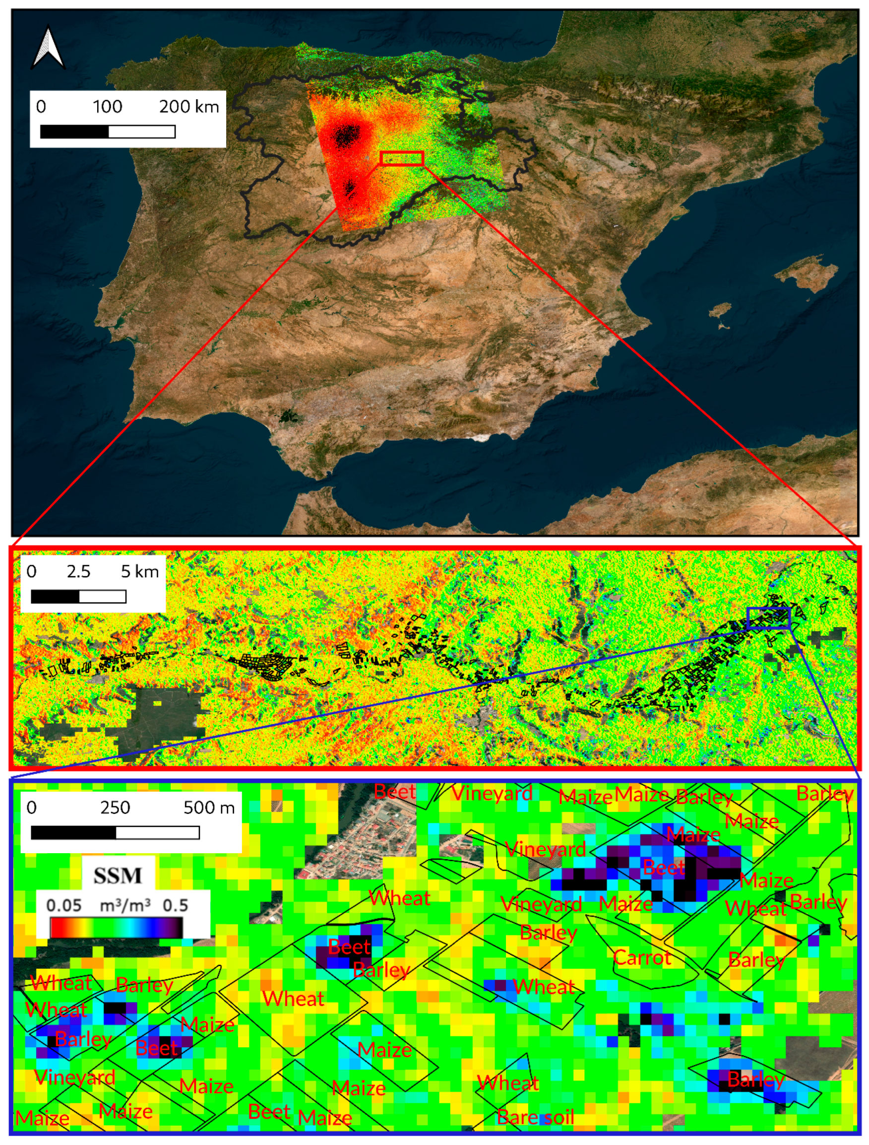Figure 4 shows an SSM map of the Castilla y León region generated with the SMOSAR software, together with the field boundaries of the study area. In the map, dark blue pixels indicate wetter soil conditions, while dark red pixels correspond to drier areas.

2.4. Data Preparation

The dataset described in Section 2.1 was organized to evaluate (i) the influence of the vegetation phenological cycle and (ii) the impact of the time span (TS) between the irrigation end time and the S-1 acquisition on the final Overall Accuracy (OA). Acquisitions from ascending and descending S-1 orbits were also analyzed separately to assess the effect of acquisition timing on irrigation detection.

The algorithm was tested on maize, sugar beet, and sunflower fields during two periods (April–June and July–September) to account for crop development and its effect on the C-band radar response [15,18,33]. These crops are typically sown in spring and reach maturity in summer. During early growth, the backscatter coefficient is more strongly correlated with the SSM, whereas in the pre-harvest stage, this correlation weakens due to the increasing contribution of volume scattering [30,34]. S-1 acquisitions affected by precipitation over the study sites were discarded, as rainfall close to the satellite overpass hampers the separation of irrigated and non-irrigated fields [14].

Regarding the effect of the time span TS, it is expected that irrigated fields maintain higher SSM levels than non-irrigated fields for a limited period [35], leading to a decrease of the OA of the classification as TS increases [18]. To analyze this effect, the 6-day S-1 revisit cycle was divided into four TS classes (0–1.5, 1.5–3, 3–4.5, and 4.5–6 day), using a 1.5-day step corresponding to the temporal separation between ascending and descending passes ($~36$ h). Based on each irrigation end time, recorded events were assigned to one of these four TS classes.

A further decision concerned irrigation events occurring only a few hours before the S-1 passage. Le Page et al. (2020) [18] showed that irrigation amounts below $10$ mm per event are difficult to detect. Therefore, only events exceeding $10$ mm were retained and assigned to the first TS class (0–1.5 days). Such events represent less than $0.5\%$ of the total and thus have a negligible impact on the overall results.

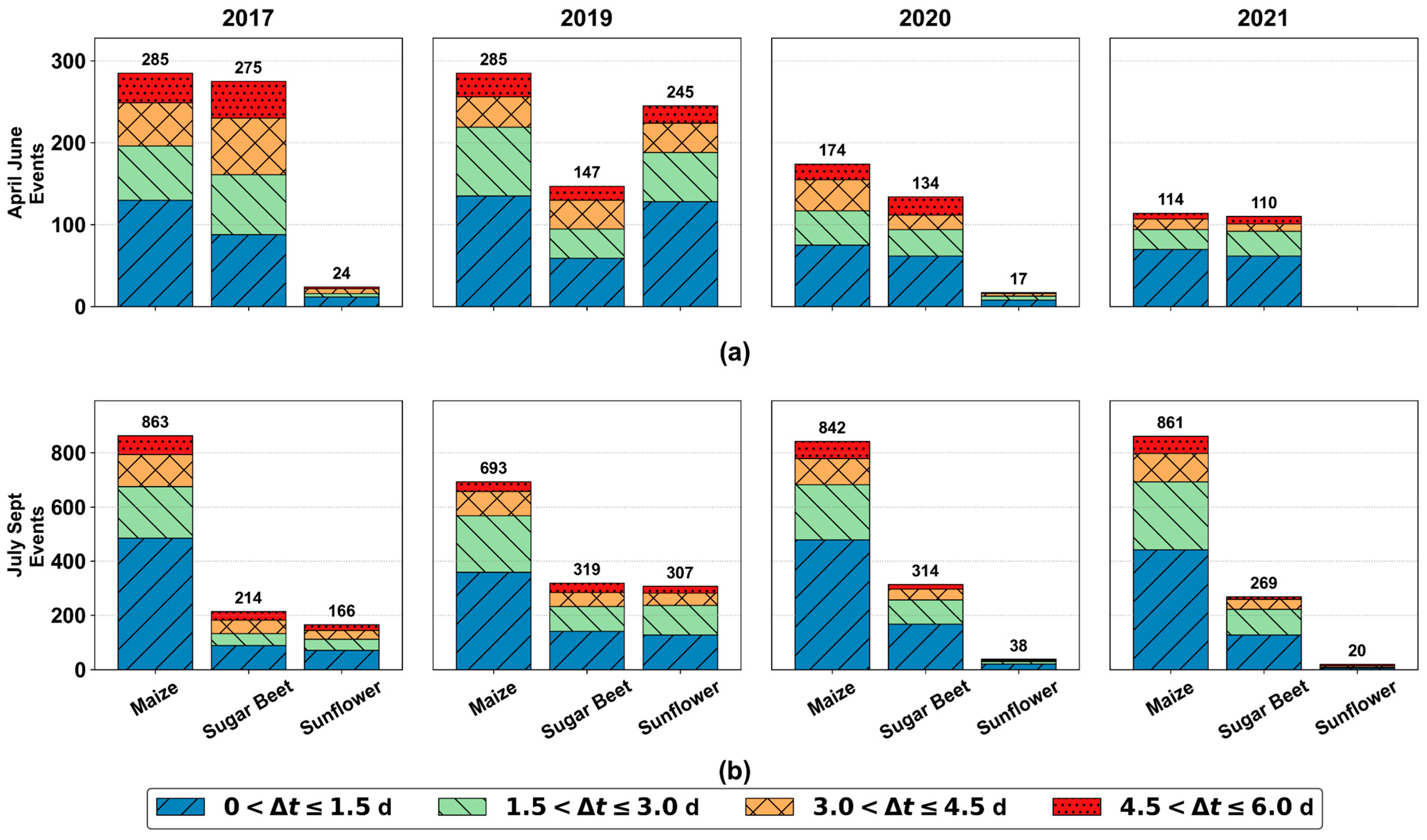
Figure 5 shows the distribution of irrigation events recorded from 2017 to 2021, categorized according to their temporal distance $\Delta t$, expressed in days, from both the S-1 ascending and descending overpasses in the April–June (a) and July–September (b) periods. Irrigations coinciding with rainfall events are excluded; therefore, the events depicted in the graph represent only those remaining after filtering out rainy dates.

Finally, the fields to be analyzed were selected based on the SSM maps spatial resolution with respect to the characteristics of the plots. Balenzano et al. (2022) [14] demonstrated that $~100$ m resolution maps effectively capture the spatial variability induced by non-uniform irrigation, outperforming coarser-resolution products. However, most fields in the study area host more than one crop, introducing heterogeneity in irrigation practices. To mitigate this effect, we selected only fields with at least $50\%$ of their area covered by the same crop and a minimum effective area of $1$ ha.

2.5. An Adaptive Classification Approach

The Constant False Alarm Rate (CFAR) detector identifies targets against clutter by means of a sliding window, where the cell under test (CUT) is compared to the statistics estimated from the surrounding reference cells (clutter). A detection is declared when the CUT exceeds a threshold set to achieve a prescribed false alarm probability [36,37]. In the current SSM application, “targets” are pixels wetter than the local background (indicating irrigation), while “clutter” corresponds to the non-irrigated background within the CFAR window. Let $t{h}_{SSM}$ denote the local threshold for a given pixel and $f_u\left(u\right)$ the PDF of the SSM clutter. The false alarm probability ($P_{fa}$) is

$$P_{fa}={\int }_{t{h}_{SSM}}^{+\mathrm{\infty }}{f}_u\left(u\right) du=1-F_u\left(t{h}_{SSM}\right)$$

(1)

where $F_u\left(·\right)$ is the corresponding cumulative distribution function (CDF). Working in terms of the CDF enables stable numerical inversion of $t{h}_{SSM}$ for either Gaussian or Gaussian-mixture models $f_u(·)$. Both the sliding-window size and the false alarm probability $P_{fa}$ are parameters influenced by the desired detection performance and spatial scale of analysis (as it is described in Section 2.6). CFAR attains the designed $P_{fa}$ when the background in the reference window is locally homogeneous. If multiple targets fall inside the reference window, the estimated clutter level is inflated, increasing false alarms. Detection is most effective when irrigated fields show a strong local SSM contrast; conversely, post-event evaporation, multiple irrigated parcels in the window or variability in applied water reduce separability. Even in mildly non-homogeneous scenes, CFAR generally provides a robust, scene-adaptive threshold [38].

In practice, the CFAR background around each CUT is not a single population, as it comprises several locally homogeneous sub-regions (fields/parcels), each with its own mean SSM (and often distinct variance). The SSM-related observable $u$ is approximately Gaussian within a parcel, with the mean significantly larger than standard deviation. This behaviour arises from the multi-look and multi-temporal normalization in STCD [29], resulting in near-Gaussian fluctuations of SSM at the parcel level. Pooling these parcel-wise Gaussians with different parameters produces a finite Gaussian mixture for the marginal clutter distribution [39]. This motivates modelling $f_u(·)$ as a Gaussian Mixture Model (GMM), fully consistent with CFAR local, data-driven estimation.

The clutter distribution of the SSM-derived observable $u\in \mathbb{R}$ is modelled with a $K$-component Gaussian mixture:

$$f_u\left(u\right)={\displaystyle \sum _{i=1}^K}{\pi }_i\mathcal{N}\left(u \right| {\mu }_i,{\sigma }_i^2), {\pi }_i\ge 0, {\displaystyle \sum _{i=1}^K}{\pi }_i=1$$

(2)

where ${\pi }_i$ are the mixing weights, and each component $\mathcal{N}(u\mid {\mu }_i,{\sigma }_i^2)$ is a univariate Gaussian. The parameter set $\mathsf{\Psi }=\left\{\right({\pi }_i,{\mu }_i,{\sigma }_i^2){\}}_{i=1}^K$ is estimated from the reference samples using Expectation–Maximization (EM). In the E-step, posterior responsibilities (the probability that a data point belongs to each component) are computed; in the M-step, $({\pi }_i,{\mu }_i,{\sigma }_i^2)$ are updated under the constant constraint ${\displaystyle {\sum }_{i=1}^K}{\pi }_i=1$ to maximize the log-likelihood. Iterations stop when the log-likelihood increment falls below a tolerance, or a maximum number of iterations is reached [40]. The mixture provides substantially greater flexibility than a single Gaussian and captures the parcel-level heterogeneity present in the pooled background.

The resulting mixture CDF $F_u\left(·\right)$ is a weighted sum of Gaussian CDFs. Hence, the CFAR threshold ${th}_{SSM}$ for a prescribed $P_{fa}$ is obtained by solving the monotone equation:

$${\sum }_{i=1}^K{\pi }_i \overline{\mathsf{\Phi }} \left({\displaystyle \frac{t{h}_{SSM}-{\mu }_i}{{\sigma }_i}}\right)=P_{\mathrm{F}\mathrm{A}} (\mathrm{monotone} \mathrm{in} t{h}_{SSM})$$

(3)

where $\overline{\mathsf{\Phi }}\left(z\right)=1-\mathsf{\Phi }\left(z\right)=\mathrm{P}\mathrm{r}(Z>z)$ for $Z~\mathcal{N}\left(\mathrm{0,1}\right)$. For a single Gaussian component $\mathcal{N}({\mu }_i,{\sigma }_i^2)$,

$$\mathrm{P}\mathrm{r}(U>t{h}_{SSM})=\overline{\mathsf{\Phi }} ((t_{\mathrm{C}\mathrm{F}\mathrm{A}\mathrm{R}}-{\mu }_i)/{\sigma }_i)$$

(4)

Summing over mixture weights ${\pi }_i$ yields the prescribed $P_{fa}$. The CFAR threshold ${th}_{SSM}$ is obtained by numerically inverting (3). To determine the optimal number of components, $k$, we evaluated the Root Mean Square Error (RMSE) between the actual and fitted distributions of SSM. This was done using maps that considered both the presence and absence of rainfall for $k$ values of $2$, $3$ and $4$. The analysis showed that increasing the number of components from $2$ to $3$ led to an average RMSE reduction of $~13\%$. However, adding a fourth component led to an increase in the average RMSE of $~4.5\%$, indicating potential overfitting. Therefore, we choose to set the number of Gaussian Components to $k=3$ for the entire analysis.

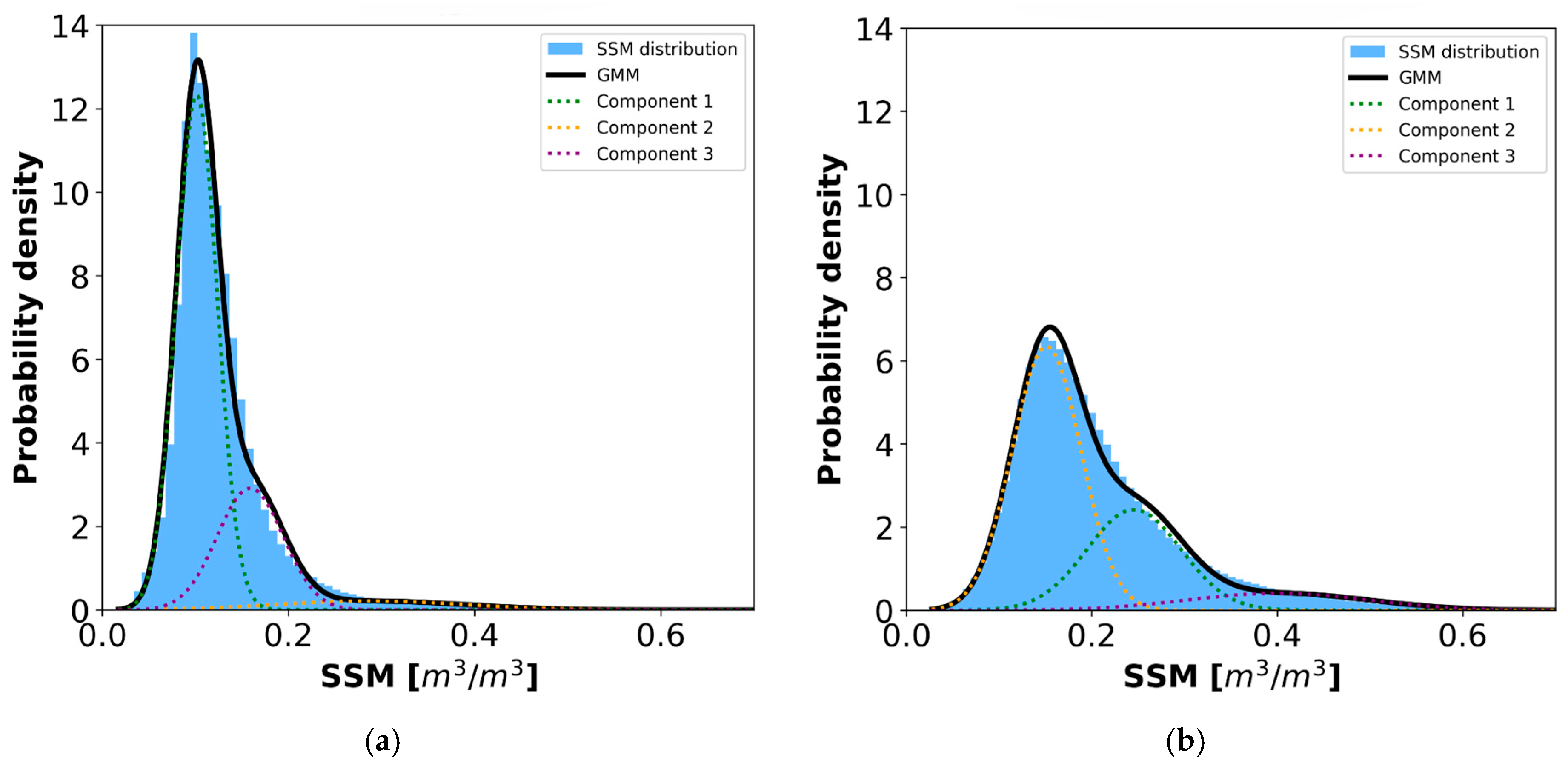
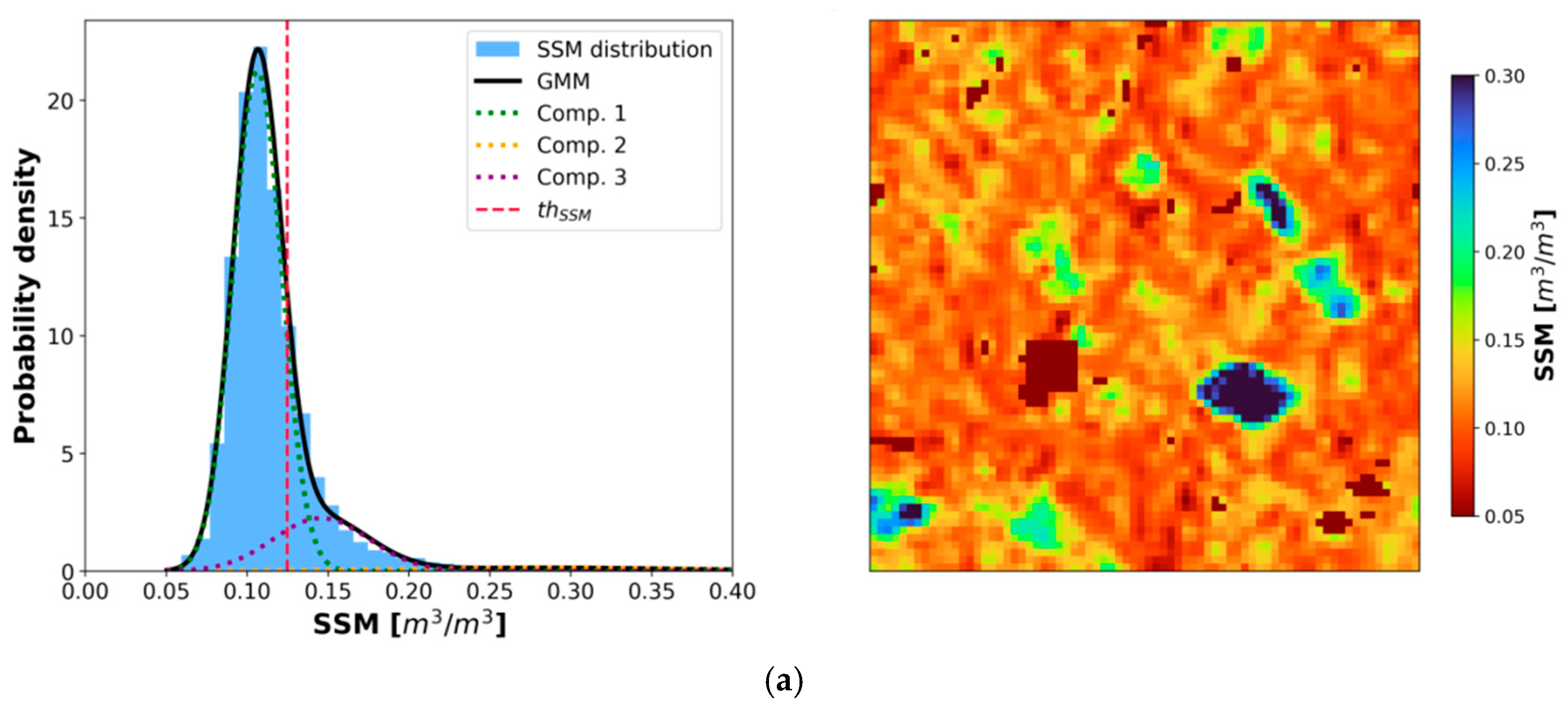
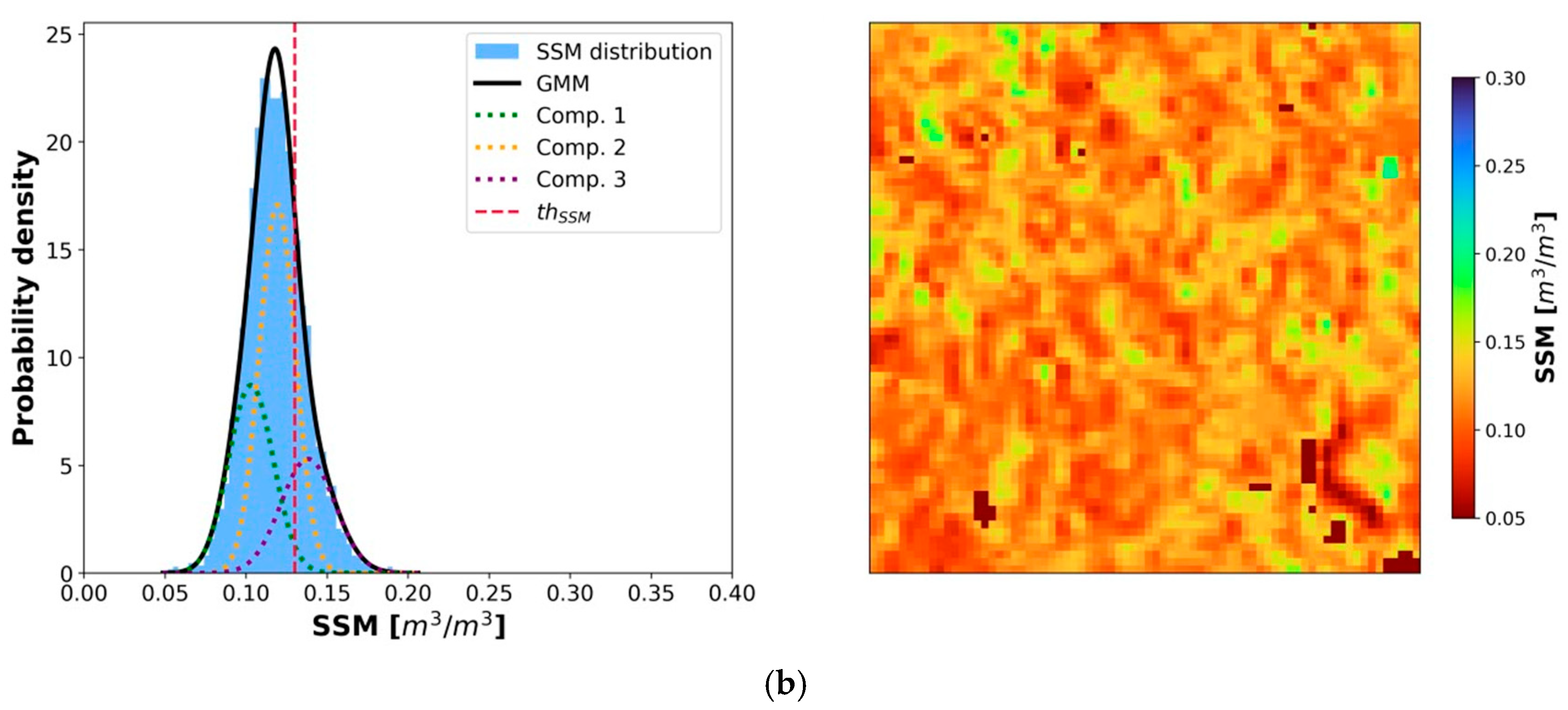
To assess how rainfall alters clutter statistics relevant to CFAR, the GMM was fitted to the distribution of SSM on dry versus rainy dates. Figure 6 shows the 2021 surface soil moisture distributions on the descending orbit: panel (a) corresponds to dry days; panel (b) to rainy days. Rainfall produces a higher mean SSM (≈$0.21$ m³/m³ vs. ≈$0.12$ m³/m³ in this example year) and a lower positive skewness (≈$1.52$ vs. ≈$2.78$, calculated with skew function of the SciPy, version 1.16.2, Python, version 3.11.2, library); the same tendency appears in other years. Because rainfall raises the background mixture mean and reduces asymmetry, the separability between irrigated pixels and clutter decreases (more tail mass near typical thresholds). This motivates a pre-CFAR rain screen, for example, by classifying a date as “rainy” when the fitted mixture mean exceeds a site-specific bound and/or the skewness falls below a threshold. In this first assessment of the irrigation detection method, the dates in which rainfalls occurred were identified on the basis of in situ meteorological data; however, the PDF skewness properties will be further investigated in future work to support an automatic rain identification tool.

2.6. Sensitivity Analysis

The input parameters needed for the implementation of the CFAR algorithm are the size of the sliding window and the $P_{fa}$. Subsequently, to aggregate at the field scale the pixel-wise classified maps, it is also necessary to set the minimum percentage of irrigated pixels to classify a field as irrigated. The field-scale aggregation process leverages the parcel border information provided by ITACyL.

Firstly, the size of the window needs to be dimensioned in order to include enough pixels for the correct modelling of the non-irrigated background clutter to mitigate the effect of multiple targets on the threshold value. Since the district also includes crops that do not require constant irrigation, and given that even the analyzed crops are not irrigated before each S-1 overpass, a larger window size ensures the inclusion of a higher proportion of non-irrigated pixels, improving the characterization of the background signal. As visible in the central panel of Figure 4 (Section 2.3), the Riaza agricultural district has a narrow and elongated shape, and at its widest and narrowest transverse points, the district measures $~4.5 \mathrm{km}$ and $~0.75 \mathrm{km}$. Consequently, setting a window equal to the minimum dimension would provide insufficient pixels for the modelling of the clutter, while setting the window dimension equal to $4.5 \mathrm{km}$ would include SSM values retrieved also in non-agricultural areas. Therefore, we tested two intermediate window sizes of $1.5 \mathrm{km}$ and $3 \mathrm{km}$.

To evaluate how the choice of the window size, the $P_{fa}$, and the field-scale aggregation percentage affects the CFAR-based detection, a sensitivity analysis was conducted on the performance metrics (Equations (5)–(10)).

$$TPR={\displaystyle \frac{TP}{TP+FN}}$$

(5)

$$TNR={\displaystyle \frac{TN}{TN+FP}}$$

(6)

$$FPR=P_{fa}={\displaystyle \frac{FP}{FP+TN}}=100-TNR$$

(7)

$$FNR={\displaystyle \frac{FN}{FN+TP}}=100-TPR$$

(8)

$$F1-score={\displaystyle \frac{2·TP}{2·TP+FP+FN}}$$

(9)

$$OA={\displaystyle \frac{TP+TN}{TP+TN+FP+FN}}$$

(10)

Here, TPR is the True Positive Rate (sensitivity/recall), TNR is the True Negative Rate (specificity), $P_{fa}$ (or FPR) is the False Positive Rate, and FNR is the False Negative Rate. OA is the Overall Accuracy and indicates the proportion of correctly classified cases, while the F1-score balances the trade-off between false positives and false negatives. TP, TN, FP, and FN denote true positives, true negatives, false positives, and false negatives, respectively. These metrics are evaluated for the detection of events in each cumulated TS interval (i.e., 0–1.5 day, 0–3 day, 0–4.5 day, and 0–6 day).

The relatively high $P_{fa}$ values tested in the analysis (i.e., $10\%, 15\%, 20\%, 25\%$) are justified by two considerations. First, a window may contain multiple targets, yet the algorithm must still correctly identify the CUT when it is irrigated, even in heterogeneous areas. Second, the backscatter contrast between irrigated and non-irrigated fields can be low, especially as time since irrigation increases; thus, a more permissive $P_{fa}$ enhances sensitivity to subtle irrigation signals and reduces false negatives.

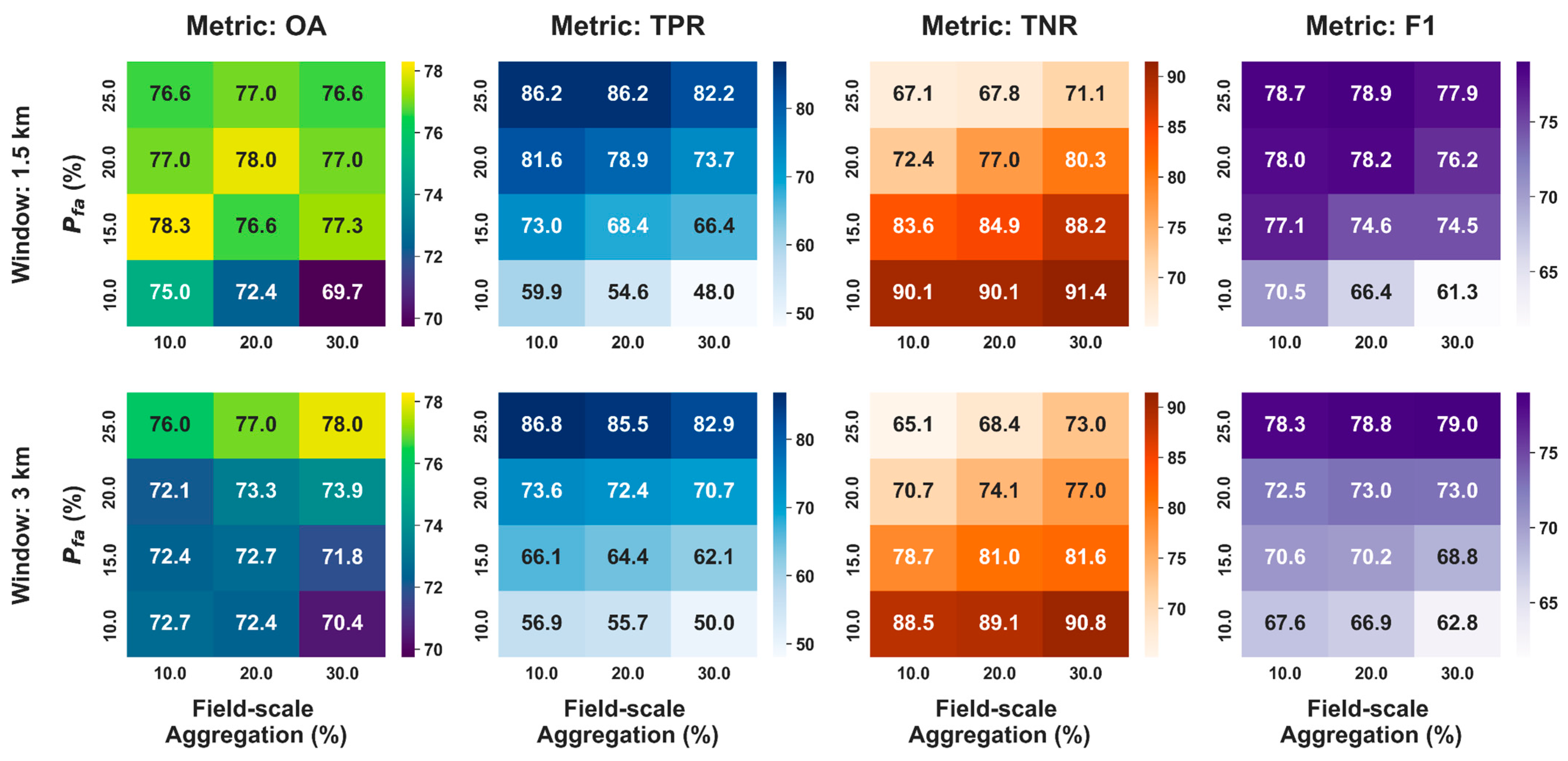
The heatmaps in Figure 7 illustrate the results of the sensitivity analysis for 2019 considering the irrigation events that take place within 1.5 days from the S-1 passage. This year represents an exemplary case, as the remaining years in the study period exhibit analogous patterns. The heatmaps show that the configuration of parameters that allows the maximization of the Overall Accuracy and the balance between True Positive and False Negative Rates is given by a window of $3 \mathrm{km}$, $P_{fa}$ equal to $25\%$ and a field-scale aggregation percentage equal to $30\%$.

And since this set of parameters was consistently optimal across all the years and orbital tracks, it was adopted for the entire analysis. To ensure statistical representativeness, this $30\%$ aggregation rule is complemented by a $1 \mathrm{ha}$ minimum area floor. Specifically, the $1 \mathrm{ha}$ threshold is applied whenever the $30\%$ rule would result in an area smaller than 1 hectare ($~4$ pixels), mitigating the risk of false detections triggered by a non-representative number of pixels.

Lastly, the TNR heatmap in Figure 7 demonstrates that a $30\%$ field-scale aggregation maintains the deviation between the observed False Positive Rate (Equation (7)) and the imposed $P_{fa}$ value within a narrow margin of $0.8$ to $3.4$ percentage points. In contrast, lower aggregation thresholds (e.g., $10\%$) result in significantly larger deviations, ranging from $1.5$ to $9.9$ points.

2.7. Demonstration of CFAR Operating

As an example, Figure 8 illustrates the application of the Gaussian Mixture Model PDF in (2) to two windows randomly extracted from the SSM map derived from the descending S-1 acquisition on 6 April 2021. In panel (a), several (4–5) visually detectable targets stand out against the background, producing a more skewed PDF. In contrast, panel (b) shows a window with heterogeneous SSM values and no visually prominent targets.

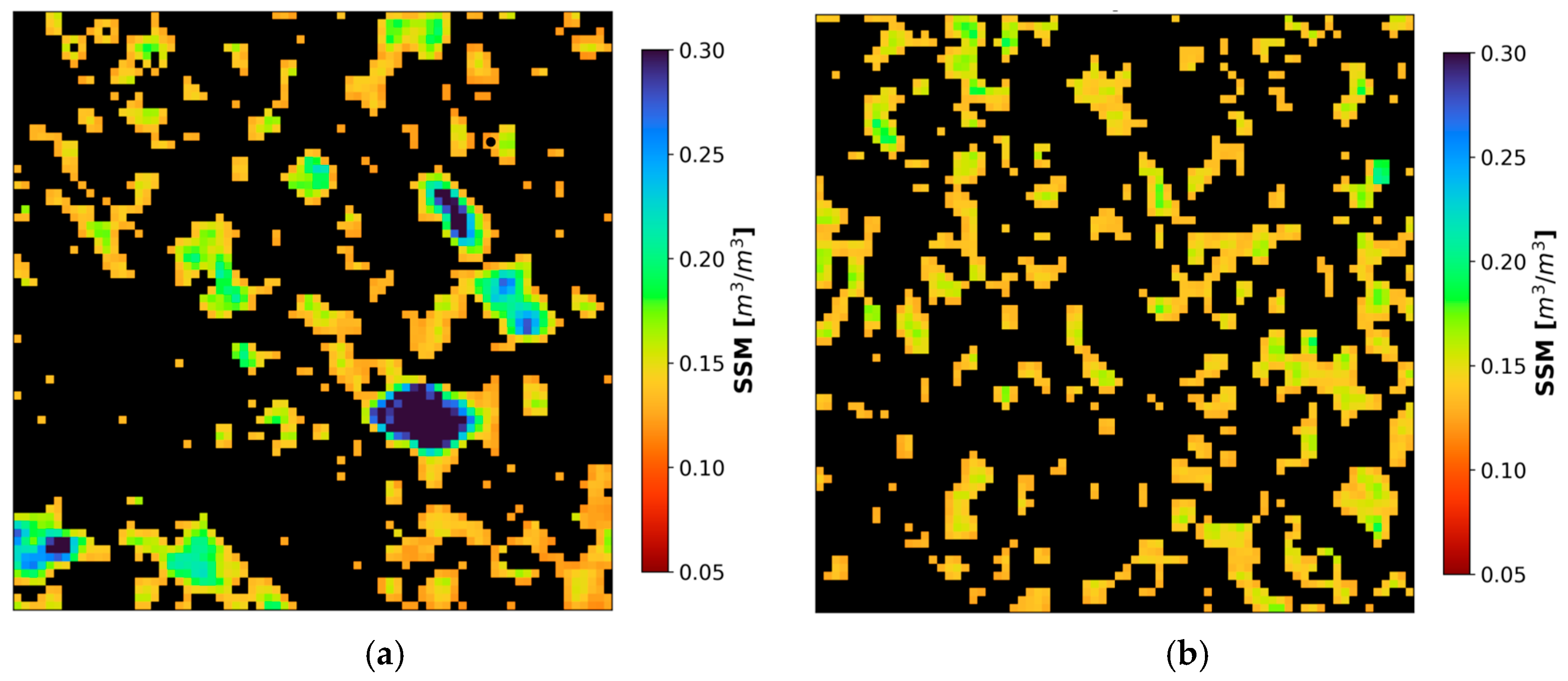
After applying CFAR to the full SSM map, the pixel-wise classification results can be visually inspected. Figure 9 shows the classification for the windows of Figure 8. Black pixels represent clutter (non-irrigated), while non-masked pixels are those classified as irrigated, and, as expected, CFAR identifies the visible targets in (a) and the high SSM pixels in (b).

As described in Section 2.3, SSM maps are masked where volume scattering dominates or where abrupt roughness changes occur. To ensure that an adequate number of pixels is available for aggregation, fields with more than $50\%$ of their pixels masked were excluded from the final classification.

The field-scale aggregation provides spatiotemporal insights into the irrigation status of the district, as classification is performed for each S-1 acquisition throughout the entire growth season. This information is leveraged to estimate the early-seasonal irrigated area ($A_{estim}$) by temporally aggregating the areas of all the detected events over the April–June period. A key advantage of using SAR-derived SSM is the ability to detect irrigation and consequently the irrigated area during the initial crop growth stages, well before full canopy development. To evaluate the relative error ($E_r$) for each year the estimated area is then compared to the actual irrigated area ($A_{act}$), which is derived from the ground data irrigation records. The relative error is calculated as follows:

$${\mathrm{E}}_{\mathrm{r}}={\displaystyle \frac{|A_{estim}-A_{act}|}{A_{act}}}·100$$

(11)

The illustrated framework was implemented using a hybrid computational environment. The CFAR detection was developed in MATLAB (version 24.2.0.2863752), and the average processing time for a single SSM map over the study area was approximately 20 min. The subsequent statistical analysis, performance metrics evaluation, and data visualization were conducted in Python (version 3.11.2). Specifically, leveraging the libraries numpy (version 2.4.4) and pandas (version 2.3.3), then geopandas (version 1.1.1), and Rasterio (version 1.4.3) for spatial data processing, scipy.stats (version 1.16.2) and sklearn.metrics (version 1.7.2) for statistical evaluation, and matplotlib (version 3.10.7) and seaborn (version 0.13.2) for graphical representation. The analysis was performed on a DELL workstation (Dell Technologies, Round Rock, TX, USA) equipped with two 32-core AMD EPYC 9334 processors (Advanced Micro Devices, Inc., Santa Clara, CA, USA) and 512 GB of DDR5 RAM, running on a Linux 6.1 kernel (The Linux Foundation, San Francisco, CA, USA).

3. Results

3.1. Detection of Irrigation Events with CFAR

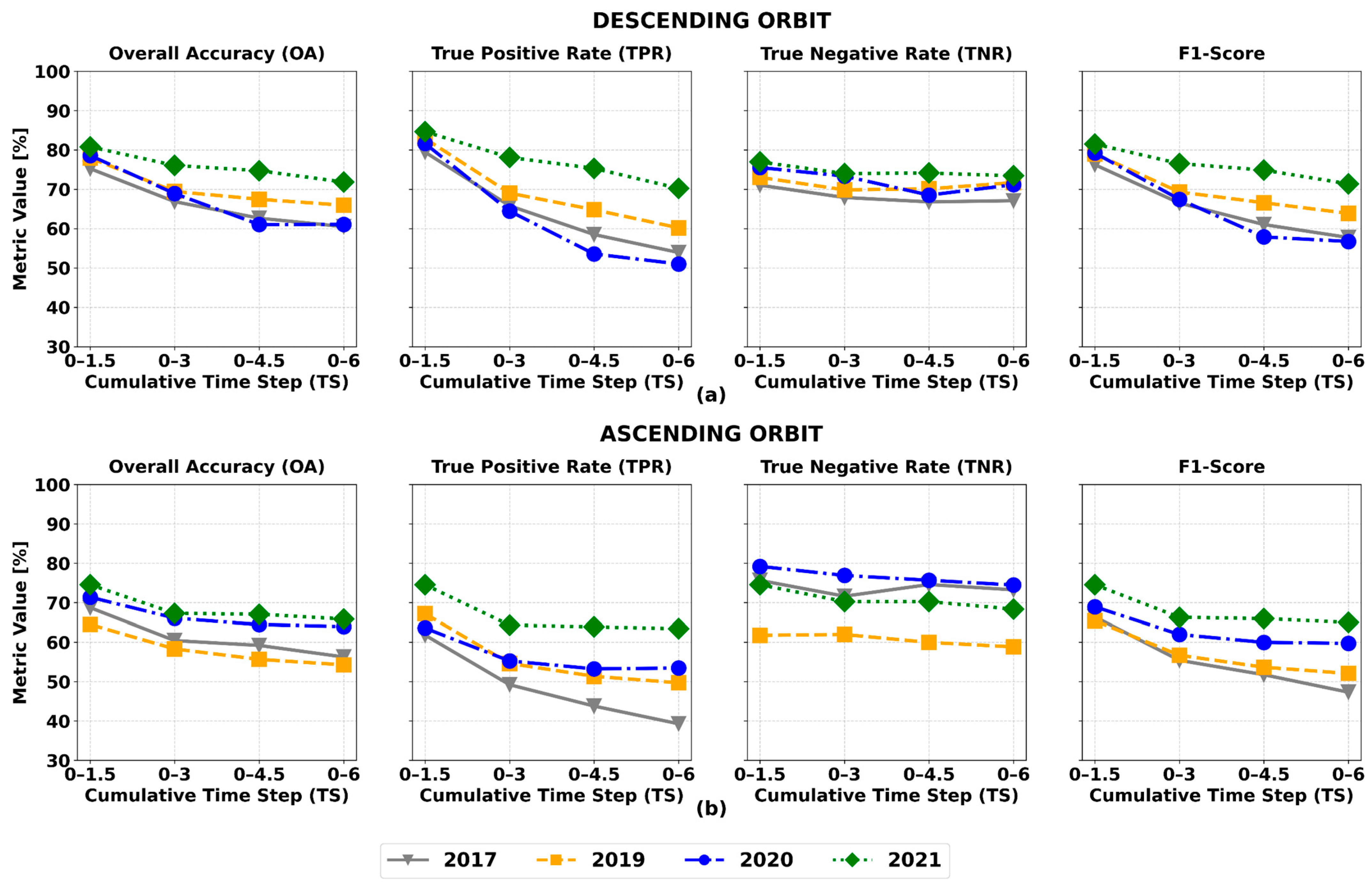
Figure 10 shows the Overall Accuracy, True Positive Rate, True Negative Rate, and F1-score associated with the detection of irrigation events during the April–June period in 2017, 2019, 2020, and 2021. Panel (a) reports results from descending acquisitions ($~6$ a.m.), while panel (b) shows the corresponding results from ascending acquisitions ($~6$ p.m.).

A clear variability in performance is observed across time spans (TS), years, and acquisition orbits. In both panels, the Overall Accuracy reaches its highest values for irrigation events occurring in the first TS and declines in the subsequent ones. For descending acquisitions, the average maximum OA is approximately $78\pm 2\%$, with a mean minimum of about $65\pm 5\%$. And, for ascending acquisitions, the mean maximum OA is around $70\pm 4\%$, and the minimum is about $61\pm 5\%$.

The differences between the two acquisition geometries are also reflected by the TPR, whose mean maximum value reaches $~82\pm 2\%$, for descending overpasses and only $~66\pm 5\%$ for ascending ones.

Regarding the FPR, its mean value during the first TS is $~26\pm 5\%$ for both orbits. This value, as illustrated in the sensitivity analysis, is close to the $P_{fa}$ used to define the CFAR threshold, thanks to the field-scale aggregation percentage equal to $30\%$. Moreover, unlike OA and TPR, the mean FPR shows only a negligible increase of approximately $4$ percentage points over the entire 6-day TS.

Conversely, for the July–September period, when crops are in their mature growth stage, classification results (omitted from the figures for brevity) follow the same qualitative trend, with the highest OA in the first TS and better performance in the early morning, but with markedly lower values than in the earlier crop stage. In this case, the mean maximum OA is $~56\pm 2\%$ and $~52\pm 5\%$ for the $6$ a.m. and $6$ p.m. acquisitions, respectively.

3.2. Comparison with K-Means Clustering

The performances of the CFAR-based detection method have been compared to the results obtained by performing the pixel-scale classification of the SSM maps using K-means clustering, which has already been employed for the detection of irrigated areas [19]. K-means is a widely used, robust and unsupervised algorithm that divides the dataset into $k$ clusters based on the minimization of the Euclidean distance between the point and the centroid of the clusters [40]. In this application, both $k=\{2,3\}$ were tested, and, since the mean silhouette of the clusters was higher than the one obtained for $k=3$ (i.e., respectively $0.75$ and $0.68$), $k$ was set equal to $2$ [41]. Furthermore, to maintain conditions analogous to the proposed method, the same field-scale aggregation percentage was applied. 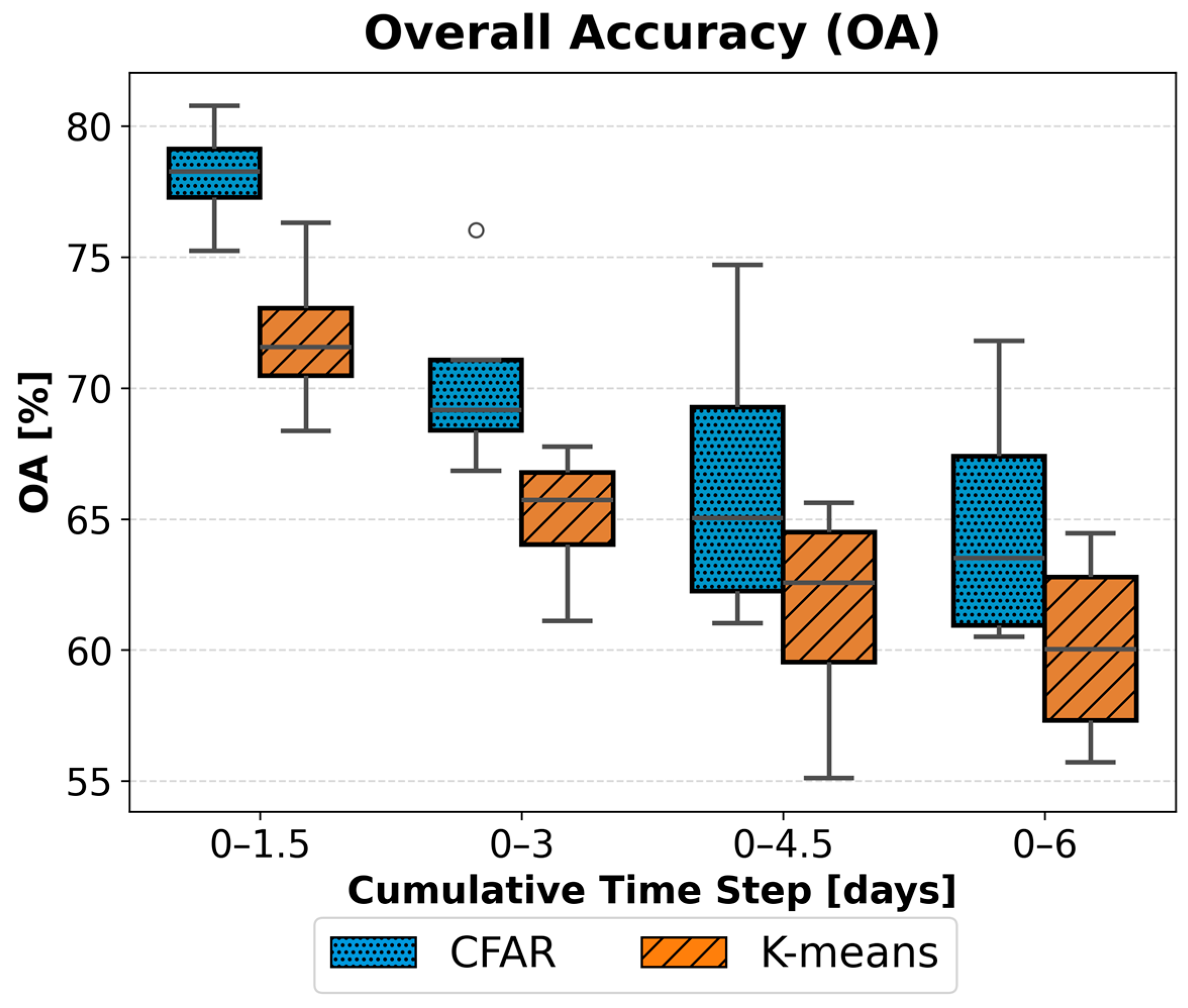Figure 11 shows the comparison between the OA obtained with CFAR and the K-means clustering for the descending orbit acquisitions. The boxplots summarize the variability of the OA obtained with the two approaches over the four analyzed years, showing that CFAR provides superior performances, especially for the irrigation events that take place within 3 days of the S-1 acquisition.

3.3. Early-Season Irrigated Area Estimation

The results of the early estimates of the irrigated area are shown in

Table 1. Comparison between the actual irrigated area ($A_{act}$) and the estimated irrigated area ($A_{estim}$) from both the descending and ascending acquisitions and their relative error.

Year	${\mathit{A}}_{\mathit{a}\mathit{c}\mathit{t}}$ [ha]	${\mathit{A}}_{\mathit{e}\mathit{s}\mathit{t}\mathit{i}\mathit{m}}$ (DSC) [ha]	${\mathit{A}}_{\mathit{e}\mathit{s}\mathit{t}\mathit{i}\mathit{m}}$ (ASC) [ha]	${\mathit{E}}_{\mathit{r}}$ (DSC) [%]	${\mathit{E}}_{\mathit{r}}$ (ASC) [%]
2017	324	333	319	2.8	1.5
2019	435	454	446	4.4	2.5
2020	326	338	344	3.7	5.5
2021	227	202	198	11.0	12.7

, which reports the actual irrigated areas ($A_{act}$) and the estimated irrigated areas ($A_{estim}$) for both descending and ascending passes, and their corresponding relative errors ($E_r$).

Overall, the average relative error ($E_r$) across all years is approximately $~5.5\%$ for descending acquisitions and $~5.6\%$ for the ascending ones. In most cases, the irrigated area tends to be overestimated, primarily due to the occurrence of false alarms. Exceptions include underestimations in 2021, considering both the ascending and descending acquisitions ($~11.8\%$), and 2017, where a slight underestimation is observed considering the ascending acquisitions.

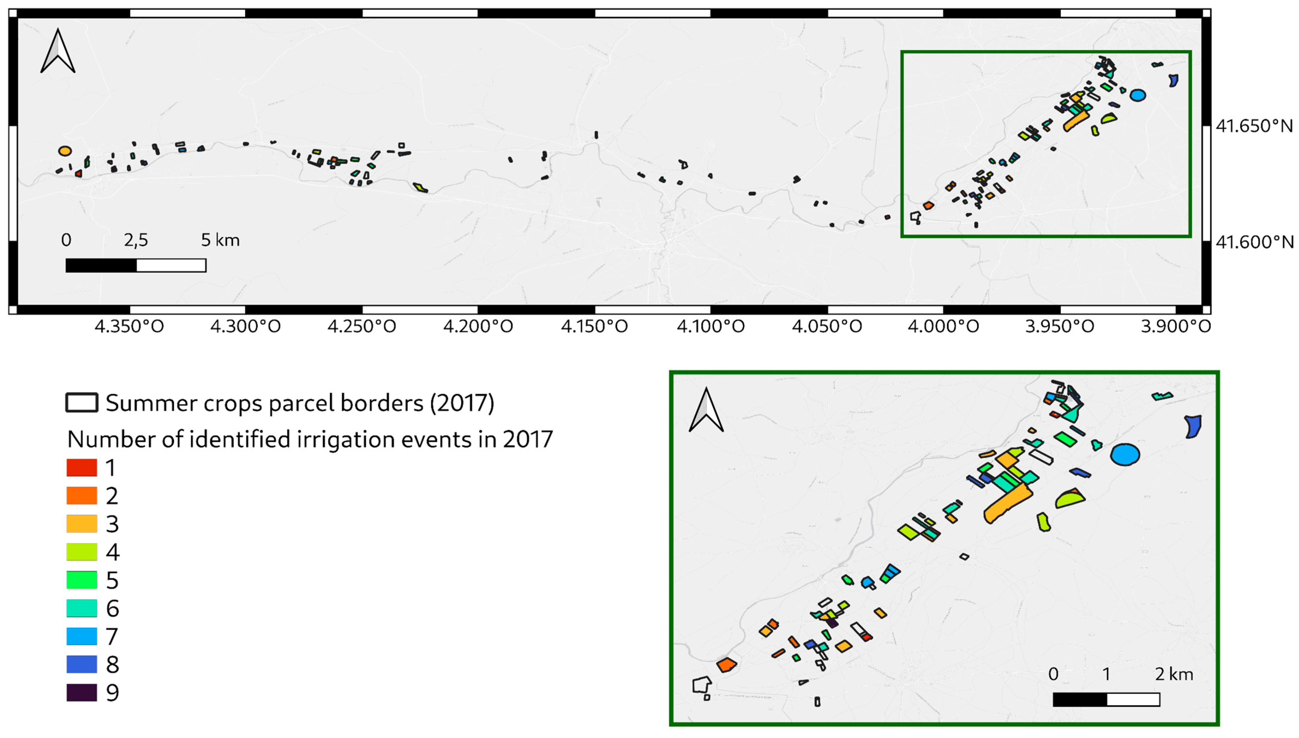
Figure 12 presents the 2017 seasonal map of irrigated areas derived from descending orbit SSM products. The temporal aggregation of the detected irrigation events throughout the first half of the growing season also incorporates the information on the total number of irrigation events detected per field. The color scale represents the irrigation frequency, providing a field-scale summary of seasonal activity.

3.4. Correlation Between SSM and Irrigation Depth

The proposed approach for the detection of the irrigated fields relies on the assumption that an irrigation event induces a localized, parcel-level enhancement of the SSM that enables the segmentation between irrigated and non-irrigated fields. Building on this rationale, we further investigated the relationship between the field mean SSM and the corresponding irrigation volumes. The latter were converted to irrigation depth (mm), assuming that the supplied water is uniformly distributed across the area occupied by the same crop.

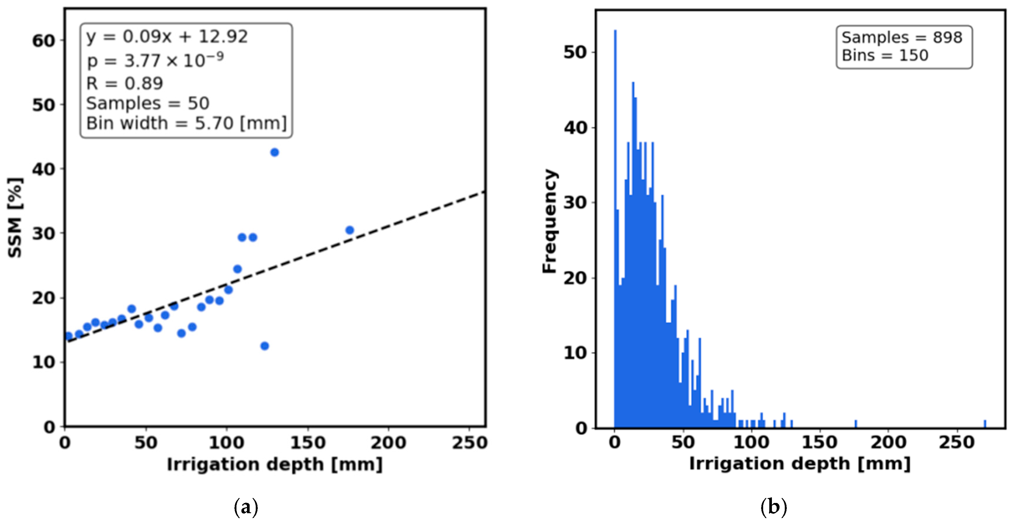
Before performing the regression analysis, irrigation depths were grouped into equally spaced bins ($~5 \mathrm{mm}$) to ensure that each interval across the observed range was given equal weight, regardless of local sample density. This prevents the regression model from being disproportionately influenced by the highly frequent, lower depth classes visible in the histogram (Figure 13b). Following this binning procedure, the linear regression revealed a strong relationship ($R = 0.89$). This approach effectively captures the conditional expectation across the entire range by neutralizing the empirical sample density imbalance. Ultimately, this result confirms the observed sensitivity of SAR-derived high-resolution SSM maps to irrigation practices [42]. The intercept with the y-axis can be regarded as an estimate of the SSM level in non-irrigated fields.

Further research will focus on a deeper exploration of this correlation and its potential practical applications, with a focus on the integration of these findings with hydrological models to estimate irrigation volumes.

4. Discussion

The objective of this study was to assess the use of high-resolution SSM maps ($~100 \mathrm{m}$), derived from S-1 and S-2 time series, for detecting irrigation at the field scale. The detection method employs the CFAR algorithm.

The results indicate that the average OA and TPR are higher for irrigation events that occur within 1.5 days of the acquisition. These metrics then decrease, reaching their minimum when considering the entire 6-day revisit time. This reduction in detection accuracy as the time from the SAR overpass increases is consistent with previous studies [18,21,43], and highlights that the SSM contrast between irrigated fields and their surroundings diminishes over time, primarily due to processes such as percolation, evaporation, and potential rainfall events, which progressively homogenize the SSM patterns [14].

Evapotranspiration also likely accounts for the differences observed between descending and ascending acquisitions. The results indicate that both the average OA and TPR are higher for descending acquisitions compared to ascending ones. This difference may be attributed to the timing of these acquisitions, which occur around $6 \mathrm{a}.\mathrm{m}.$ for descending and around $6 \mathrm{p}.\mathrm{m}.$ for ascending observations. Furthermore, observations reveal an increase in the overlap between the SSM levels of irrigated and not irrigated fields in the afternoon. This makes it easier to distinguish the two levels in the early morning.

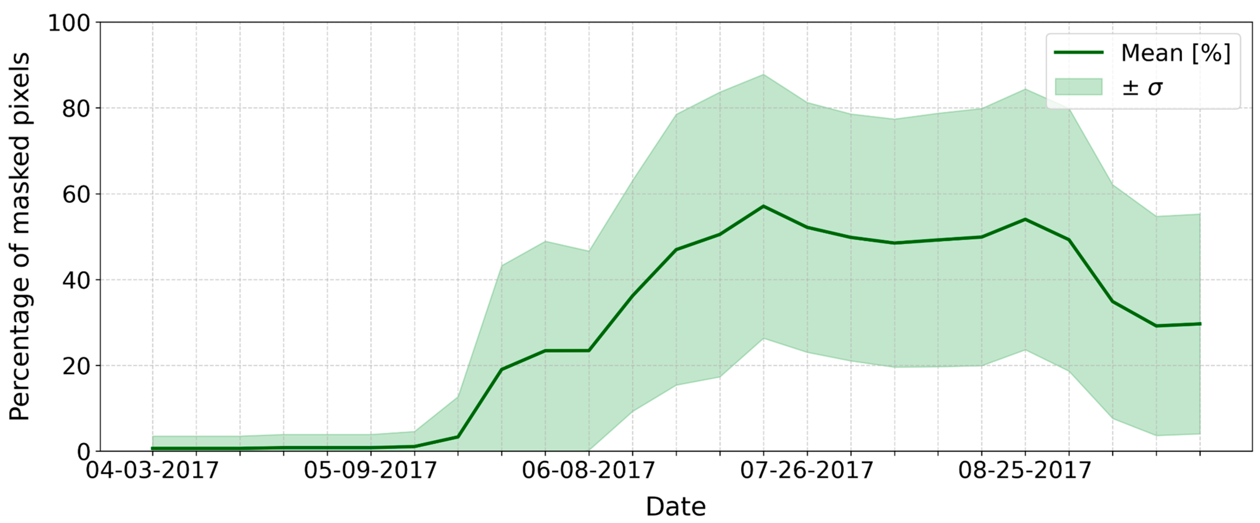
Lastly, the results indicate that between July and September, the effectiveness of irrigation detection decreases due to the stronger interference and subsequent image masking caused by dense vegetation. This occurs because the C-band SAR signal is highly sensitive to the structural and dielectric properties of vegetation [15,18,44]. As a result, SMOSAR masking becomes increasingly important from July onwards, particularly over crops such as sugar beet and sunflower. For instance, Figure 14 shows the masking trend observed over sugar beet crops in 2017 for descending satellite orbits. During the peak vegetative stage, a substantial portion of the cropped area becomes masked, resulting in a reduced number of valid pixels available for field-scale analysis. Consequently, there are often too few unmasked pixels available, which can lead to missed detections. This issue is severe with C-band systems; however, it can be mitigated by using SSM maps from L-band systems, which are less affected by the crop canopy and therefore maintain greater sensitivity to soil moisture.

The advantages of using a spatially adaptive strategy for detecting specific events are highlighted by comparing the proposed CFAR approach with K-means, a traditional clustering method. The CFAR-based method demonstrates a higher OA than K-means, particularly for events occurring within three days of the S-1 overpass. However, for events that occur beyond this three-day window, the performance difference between the two methods diminishes. This is due to the spatial homogenization of soil moisture data, which makes detection challenging for both approaches. This finding indicates that global clustering methods struggle to capture pixel-scale differences related to irrigation. In contrast, by adapting the classification threshold locally for each pixel, the CFAR algorithm effectively isolates the specific irrigation signal from the surrounding environmental noise.

Expanding the analysis from the field scale to the district scale, we explored the feasibility of estimating irrigated areas during the early crop-growth period (April to June) and the relationship between SSM and the applied irrigation volumes. Our findings regarding the estimation of irrigated areas indicate a tendency toward overestimation, primarily due to the occurrence of false alarms. However, the results for 2021 are an exception, as the total area is significantly underestimated. This underestimation is attributed to several rainfall events that coincided with S-1 overpasses. As a result, we had to exclude the affected acquisitions during the rainfall filtering stage. Nevertheless, 2021 was still included in the overall assessment because the dataset retained enough valid events post-filtering to ensure the reliable execution of the detection algorithm, which included $224$ irrigation events (see Figure 5). Finally, we assessed the feasibility of linking the observed enhancements in SSM mapping to actual irrigation depths. However, the highly skewed distribution of the sampled depths required us to first group the data into equally spaced bins to estimate the expected SSM response conditional on irrigation depth across the full range. Following this remediation, a strong positive correlation identified through linear regression suggests that the spatial adaptation of the CFAR method effectively captures variations in irrigation intensity. Further analysis remains necessary, ideally using larger and more balanced datasets, to fully establish this quantitative relationship and investigate its implications for directly retrieving irrigation volumes.

5. Conclusions and Outlooks

This study presented an unsupervised and adaptive methodology for identifying irrigation events using SAR-derived SSM data, supported by a robust and comprehensive ground-based dataset. While SSM products are well-established in the literature as reliable indicators of soil wetness linked to irrigation, this work advances the state of the art by proposing and assessing an approach for detecting irrigation events at the field scale from SSM maps at $~100$ m resolution ($~40$ m pixel size), obtained through the processing of S-1 and S-2 time series using SMOSAR software [27].

The methodology leverages the CFAR algorithm to segment irrigated and non-irrigated soils at the pixel level. The PDF adopted to characterize the SSM values is the Gaussian Mixture Model (GMM). The results were subsequently aggregated at the field scale using parcel boundary information provided by ITACyL for the Riaza irrigation district.

Although the CFAR algorithm has been widely applied for target detection in SAR imagery, this study represents a first assessment of its application to SSM maps for identifying irrigated fields. Results indicate that the detection accuracy is primarily influenced by acquisition timing, crop growth stage and the TS between the S-1 acquisition and the irrigation event. Considering all the crops irrigated during the April–June period and both the descending and the ascending overpasses, the highest average OA ($~75\pm 5\%$) is consistently achieved when irrigation occurs within $36$ h before the S-1 passage. The OA remains above $70\pm 6\%$ provided that the temporal gap between irrigation and acquisition does not exceed 3 days. A notable decline in the performance is observed from July to September and can be attributed to the dominant influence of vegetation on the C-band backscatter [44]. This highlights the potential benefit of integrating L-band acquisitions, which are less sensitive to canopy effects, and vegetation indices from optical data to monitor irrigation at later growth stages.

The proposed methodology also demonstrated significant potential for the early-season estimate of the irrigated area through the temporal aggregation of detected events. The comparison with in situ data yielded mean relative errors of approximately $5.6\%$, which is mainly due to the tendency to overestimate the total irrigated area because of the occurrence of false alarms during field identification.

Lastly, the analysis of the relationship between field-scale mean SSM and irrigation depth revealed a strong correlation confirming the sensitivity of high-resolution SSM maps to irrigation volumes.

Several directions for future improvement emerge from this study. First, the temporal dimension will be explored, for instance by enforcing temporal consistency in irrigation detection to mitigate false alarms and refine irrigated area estimates. Second, further investigations will be conducted to automate rainfall identification based on the statistical properties of the SSM distribution. Notably, also leveraging more balanced irrigation datasets, future research will evaluate the potential of exploiting the correlation between SSM and irrigation depth to quantify irrigation volumes, also in synergy with energy water balance models [23,25].

Finally, to evaluate the adaptability and transferability of the proposed methodology, future work will apply it to other agricultural regions characterized by diverse crops, management practices and irrigation systems.