Empirical Polarization Distribution Models for Use in CLARREO Pathfinder-VIIRS Intercalibration


Highlights
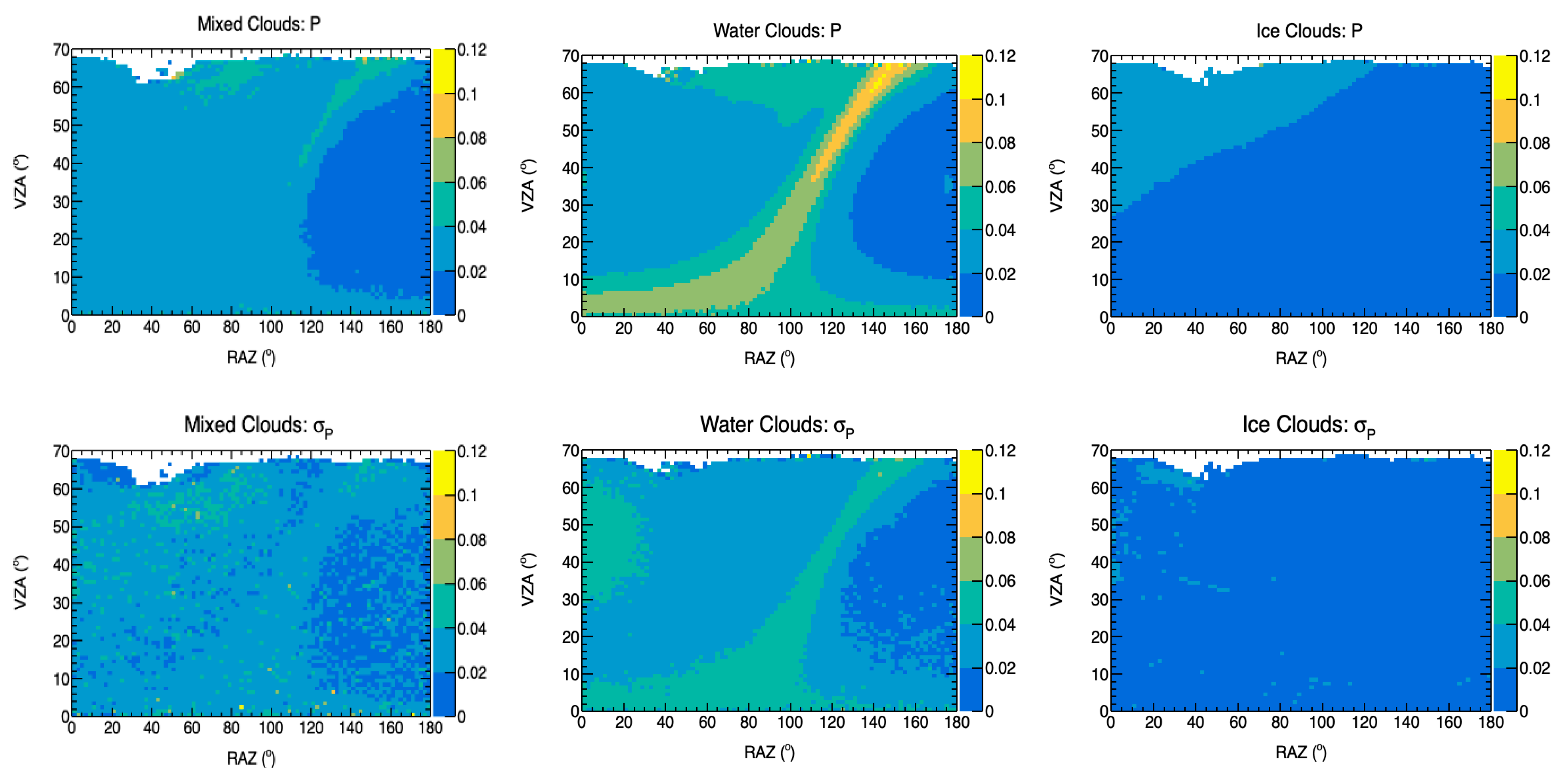
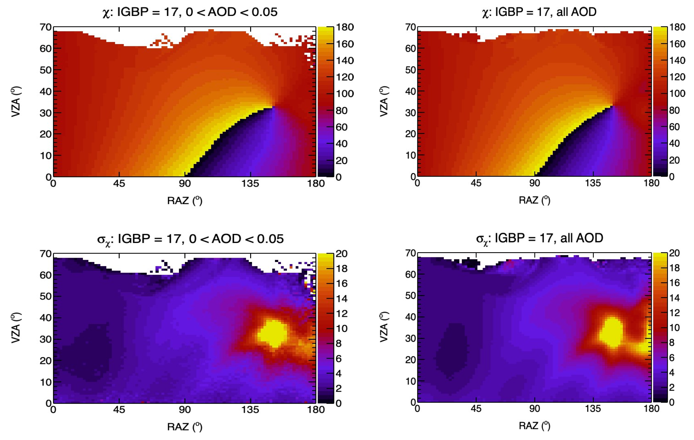
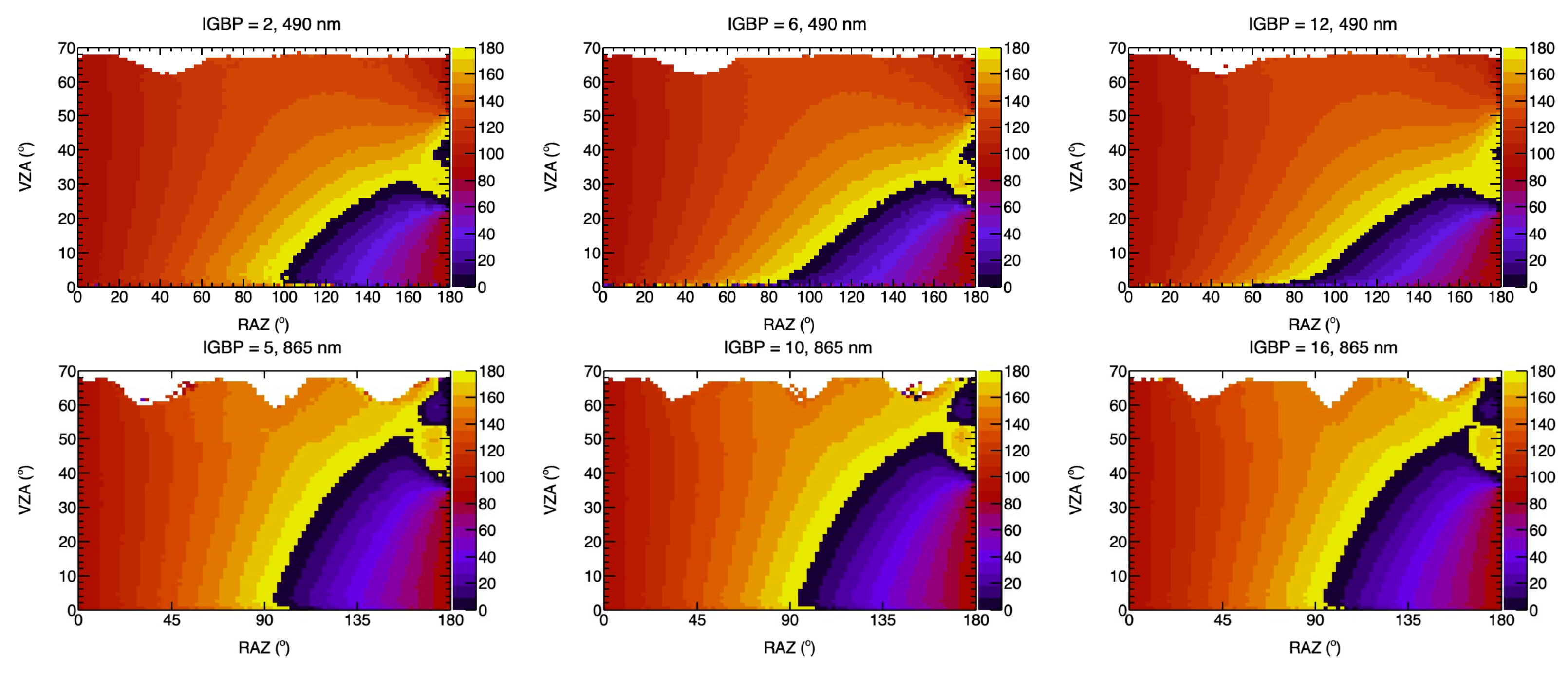
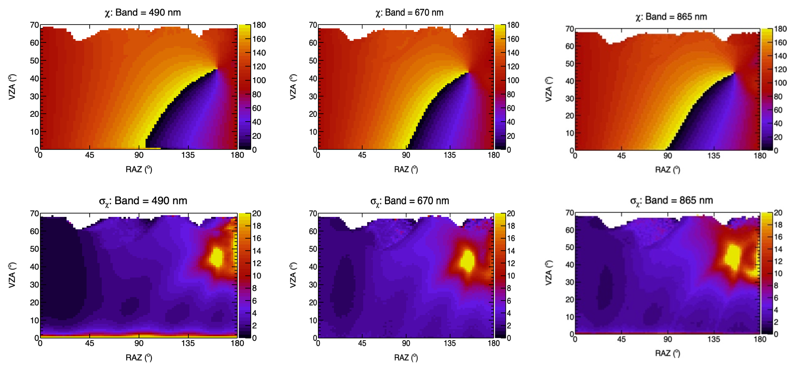
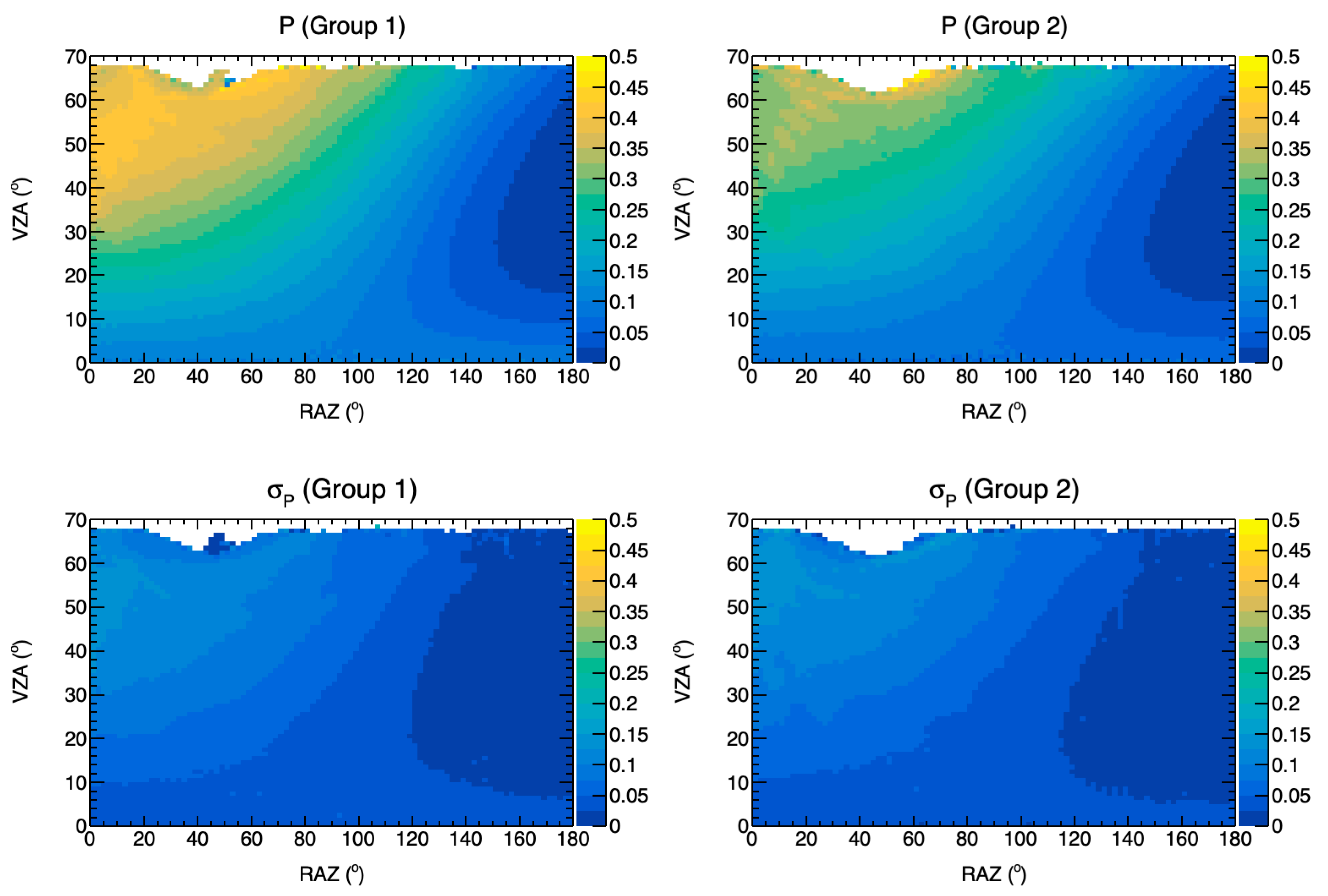
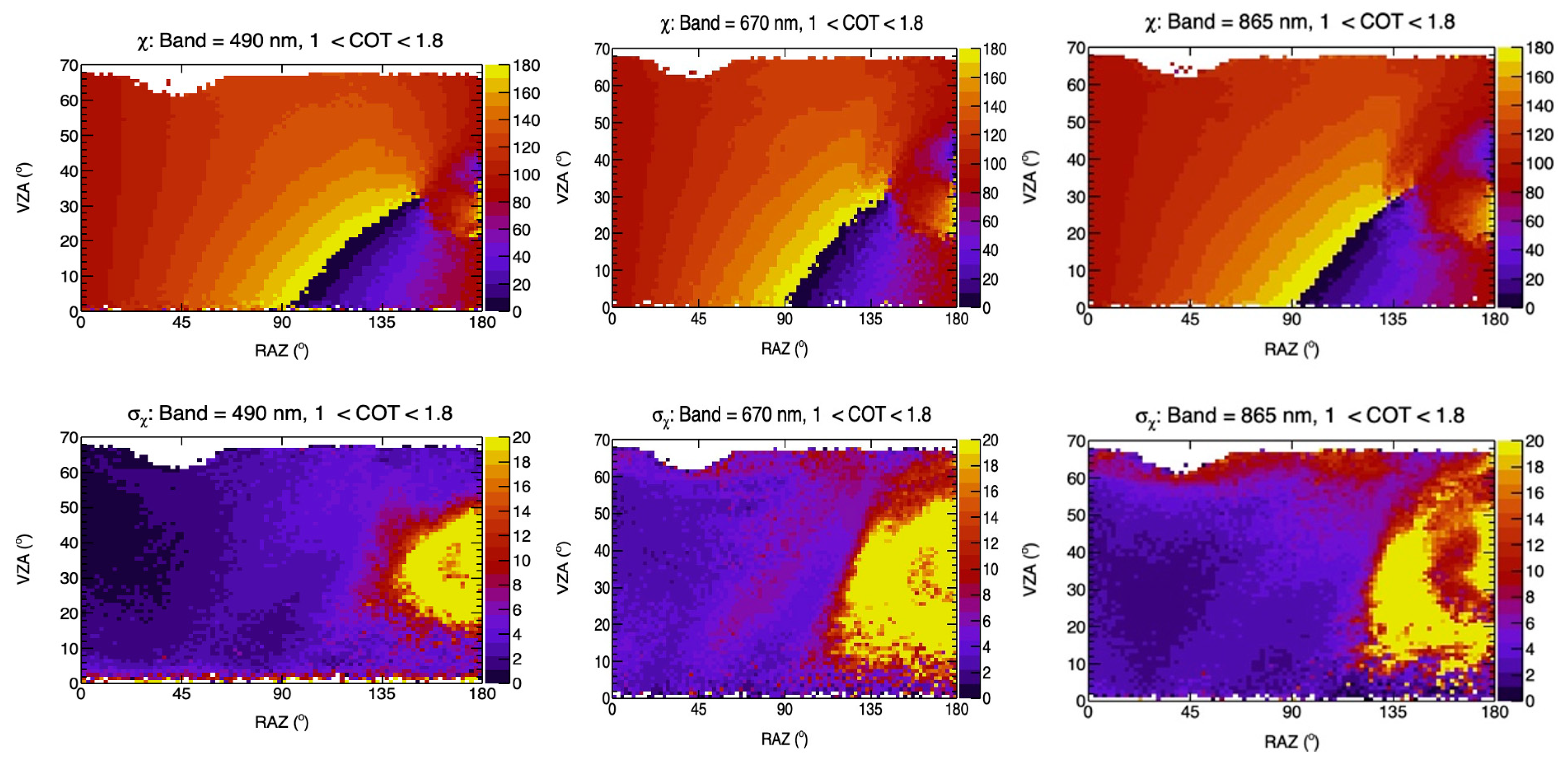
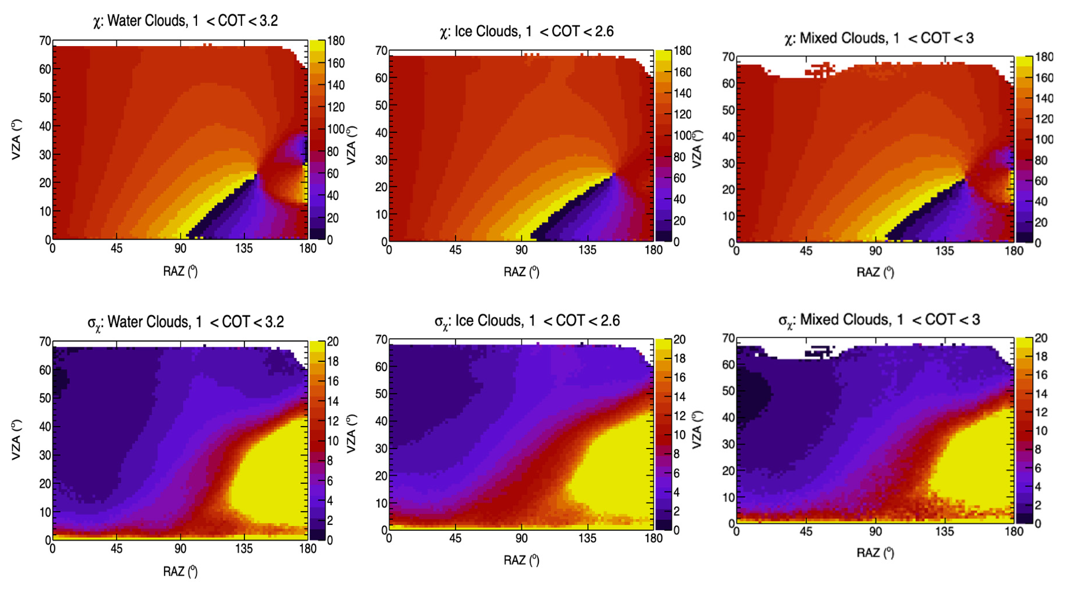
- Polarization can introduce bias in radiometric intercomparisons over polarized Earth scenes, especially for polarization-sensitive instruments like VIIRS. To mitigate this, the CLARREO Pathfinder team developed empirical Polarization Distribution Models (ePDMs) using POLDER data that characterize scene polarization using DOP and AOP as functions of scene type, geometry, and wavelength.
- The development and application of ePDMs enable more accurate intercalibration of polarization-sensitive VIIRS RSBs against CPF’s high-accuracy benchmark measurements. By selecting low-polarization scenes for comparison, the CPF team reduces systematic bias introduced by differing polarization diattenuation coefficients, improving accuracy in the radiometric intercalibration.
Abstract
1. Introduction
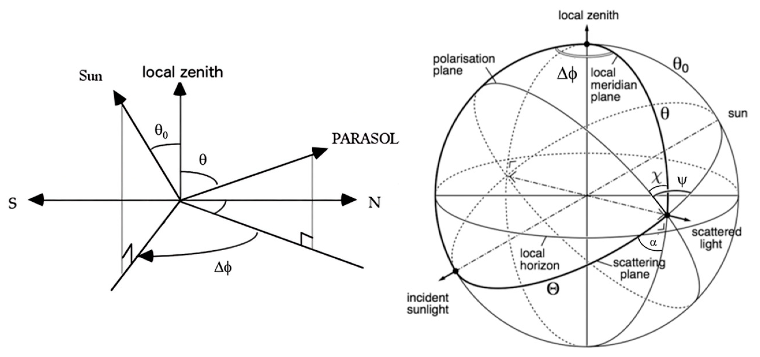
2. Polarization: Mathematical Definitions
3. ePDMs from POLDER/PARASOL Data
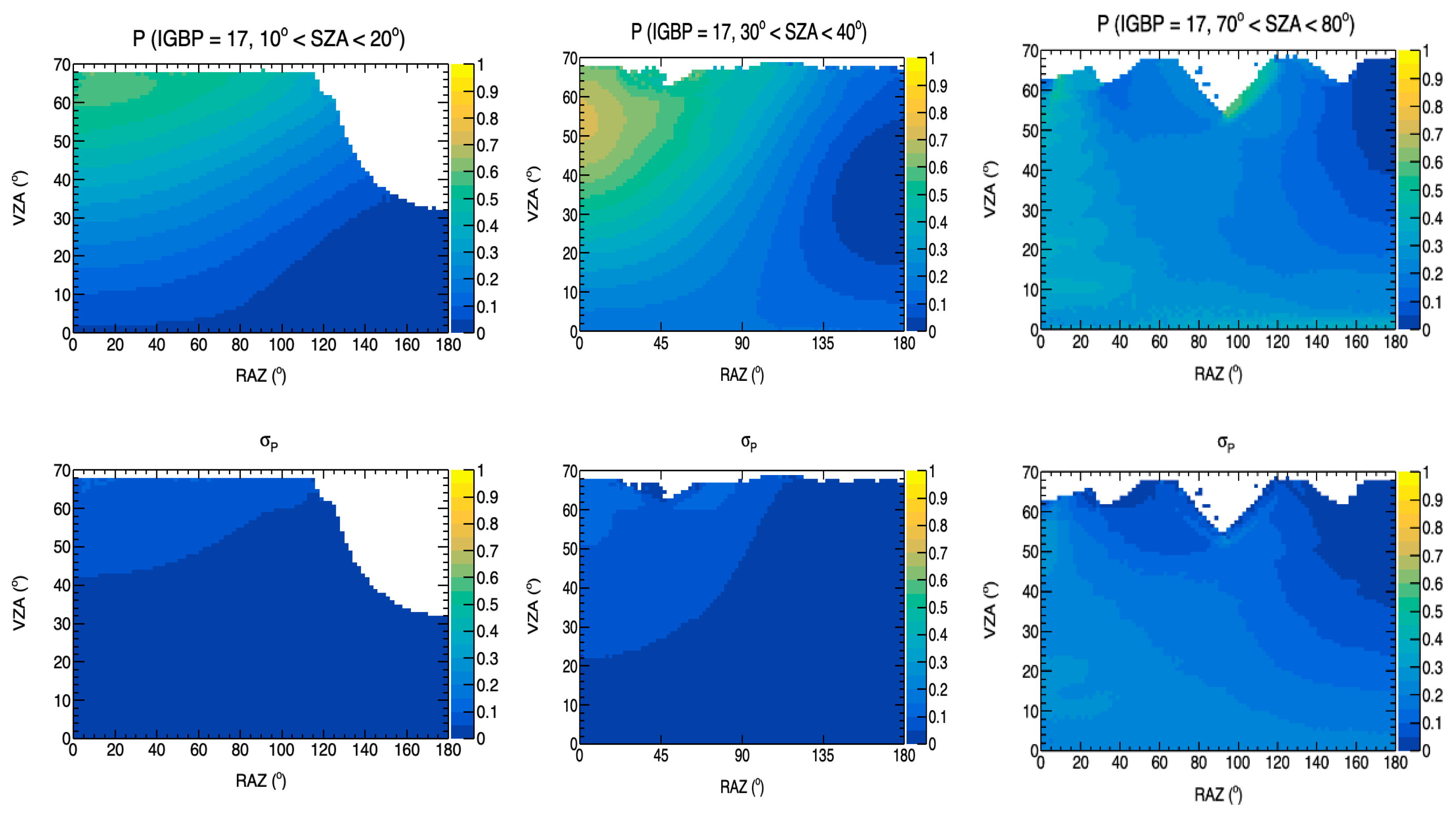
3.1. DOP ePDMs
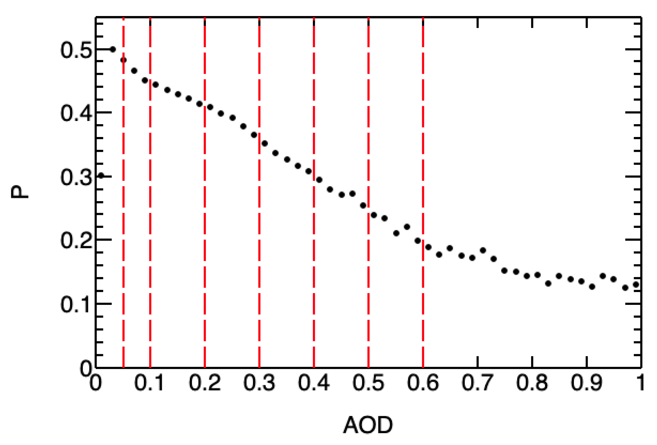
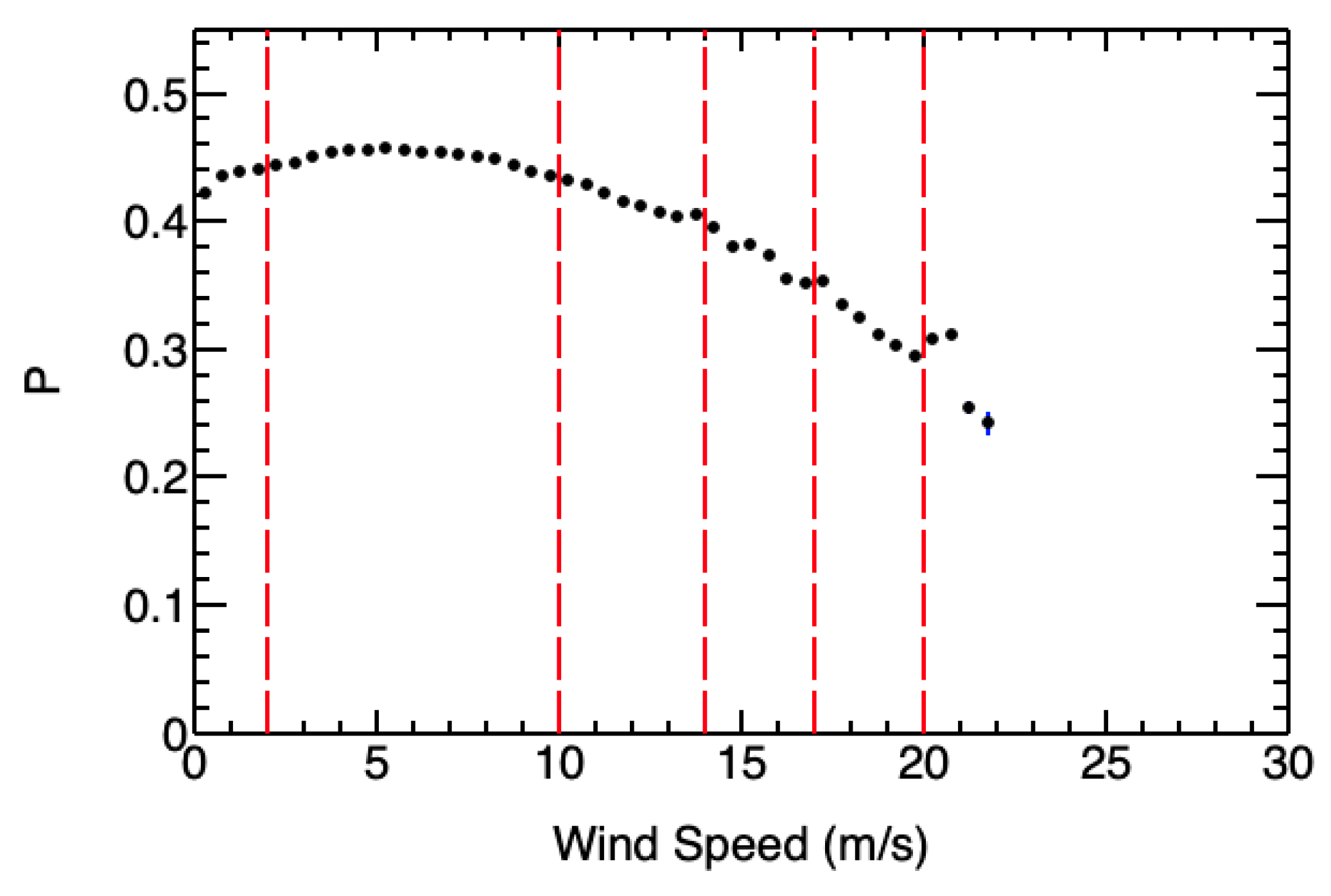
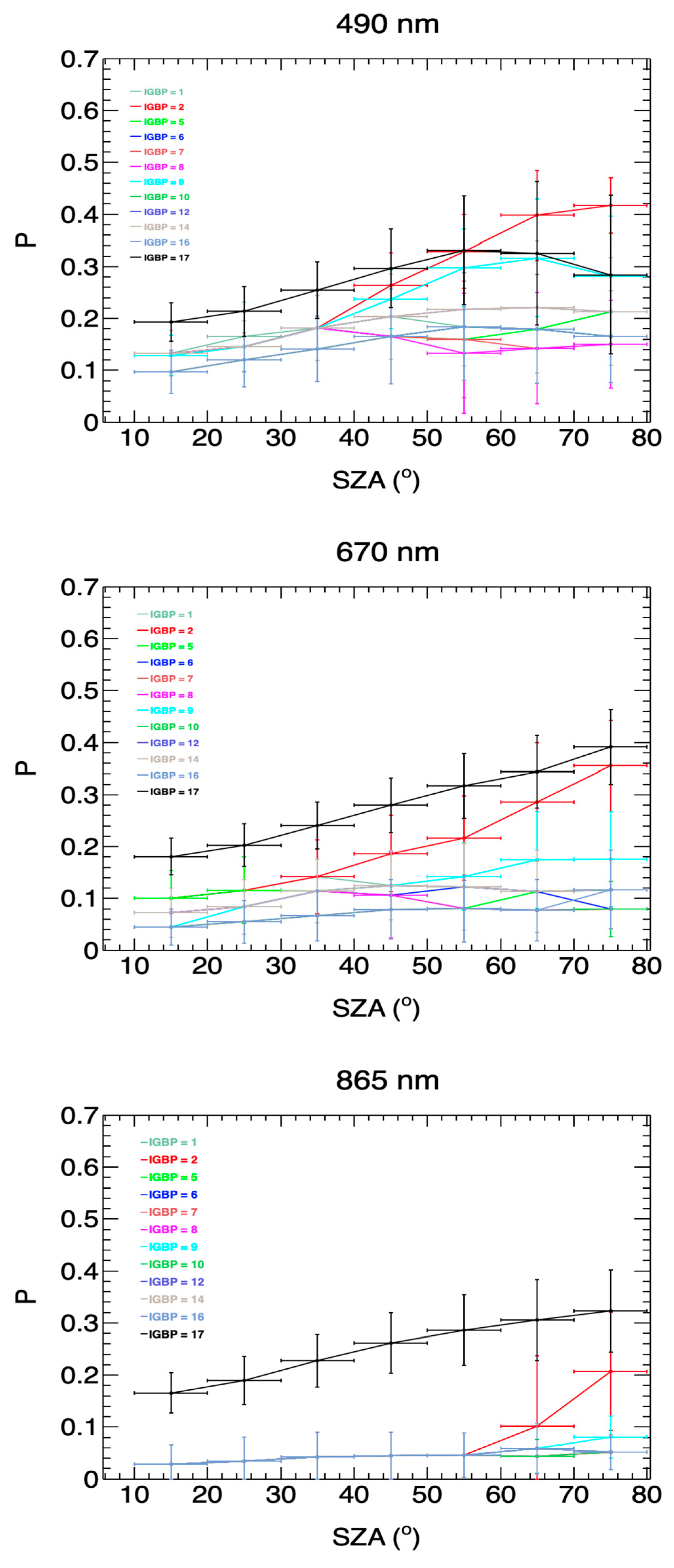
3.1.1. DOP ePDMs for Clear-Sky over Water Bodies
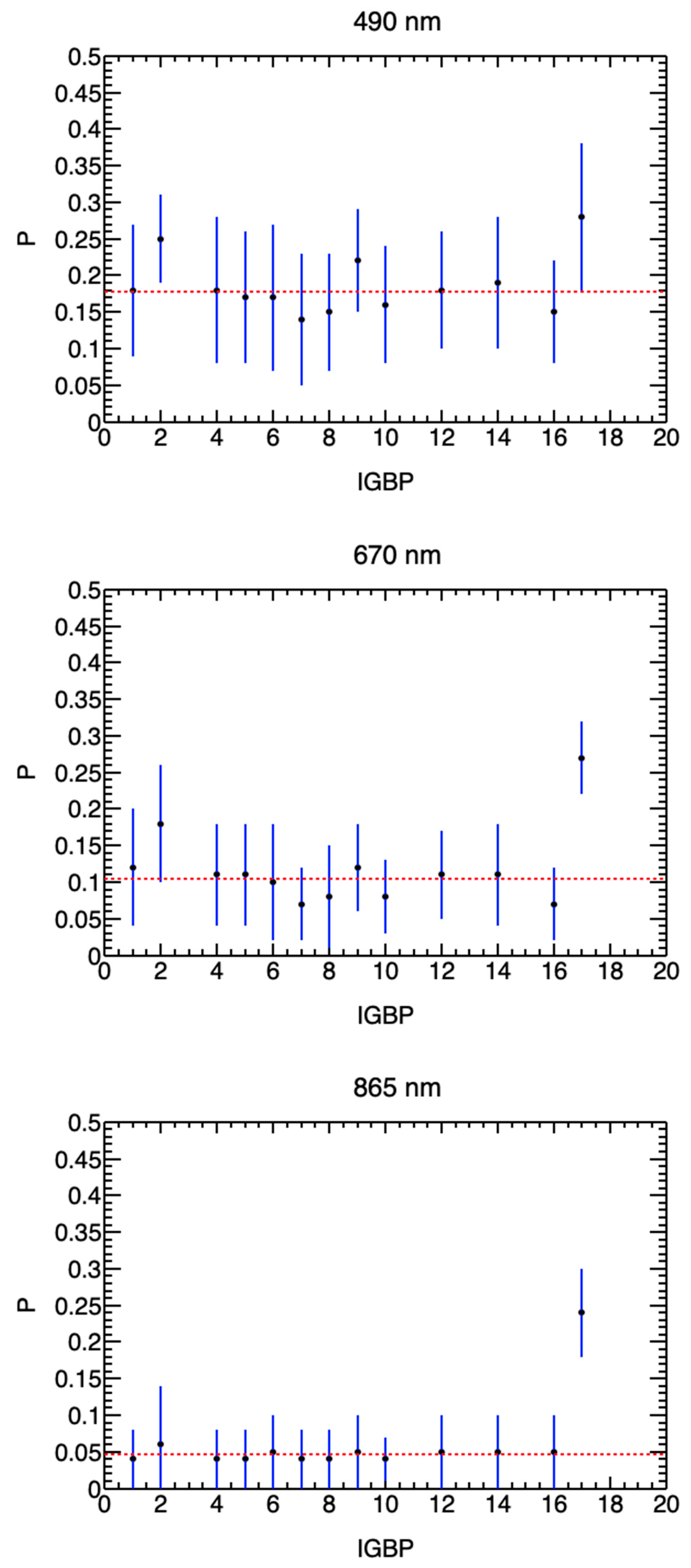
3.1.2. DOP ePDMs for Clear Sky Over Land Surfaces
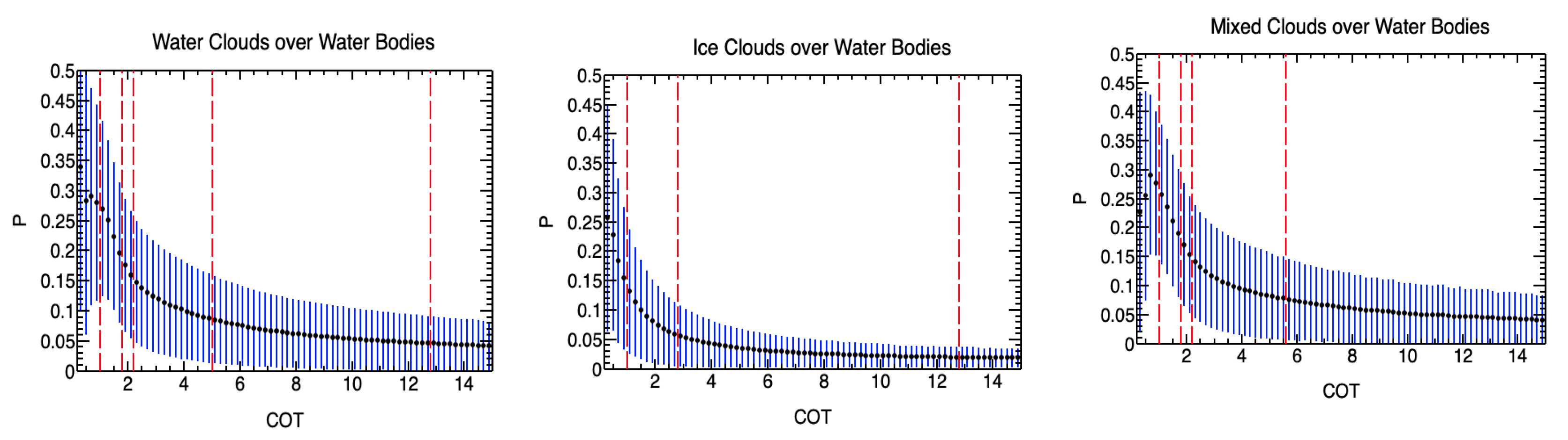
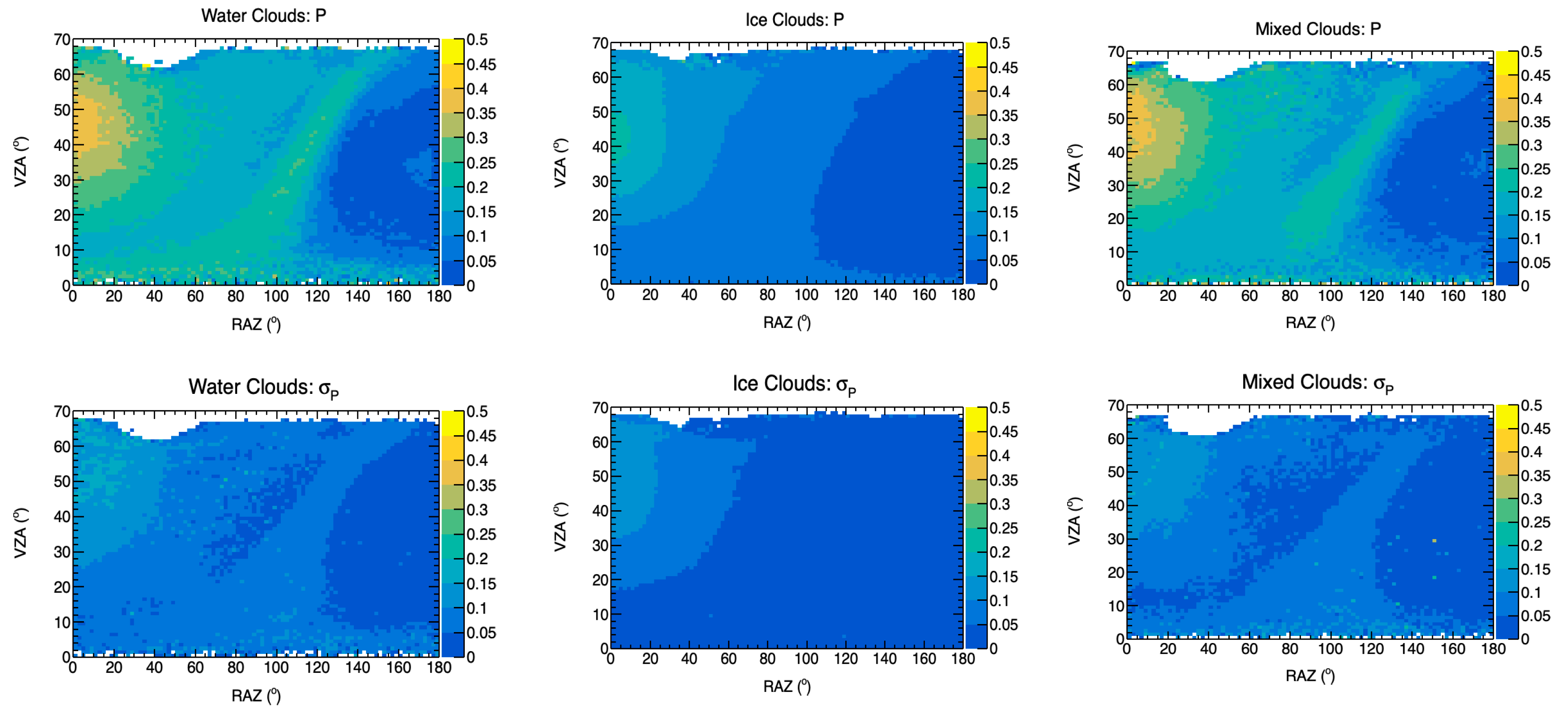
3.1.3. DOP ePDMs for Overcast Water Bodies and Land
3.2. AOP PDMs
3.2.1. Clear-Sky AOP PDMs
3.2.2. Overcast AOP PDMs
4. Sensitivity of Intercalibration to Variations in DOP and AOP
5. Conclusions
Author Contributions
Funding
Data Availability Statement
Conflicts of Interest
References
- Bhatt, R.; Shea, Y.; Wu, W.; Yang, Q.; Goldin, D.; Sun, W.; Little, M.; Liu, X.; Smith, N.; Lukashin, C. CLARREO Pathfinder as a SI-traceable reference for satellite intercalibration. In Proceedings of the SPIE 12685, San Diego, CA, USA, 23–27 August 2026; Volume Earth Observing Systems XXVIII, p. 1268507. [Google Scholar] [CrossRef]
- Shea, Y.; Fleming, G.; Kopp, G.; Lukashin, C.; Pilewskie, P.; Smith, P.; Thome, K.; Wielicki, B.; Liu, X.; Wu, W. CLARREO Pathfinder: Mission Overview and Current Status. In Proceedings of the IGARSS 2020-2020 IEEE International Geoscience and Remote Sensing Symposium, Waikoloa, HI, USA, 26 September–2 October 2020; pp. 3286–3289. [Google Scholar] [CrossRef]
- Lee, T.E.; Miller, S.D.; Turk, F.J.; Schueler, C.; Julian, R.; Deyo, S.; Dills, P.; Wang, S. The NPOESS VIIRS Day/Night Visible Sensor. Bull. Am. Meteorol. Soc. 2006, 87, 191–200. [Google Scholar] [CrossRef]
- Sun, J.; Wang, M.; Jiang, L.; Xiong, X. NOAA-20 VIIRS polarization effect and its correction. Appl. Opt. 2019, 27, 6655–6665. [Google Scholar] [CrossRef] [PubMed]
- Lukashin, C.; Jin, Z.; Kopp, G.; MacDonnell, D.G.; Thome, K. CLARREO reflected solar spectrometer: Restrictions for instrument sensitivity to polarization. IEEE Trans. Geosci. Remote Sens. 2015, 53, 6703–6709. [Google Scholar] [CrossRef]
- Goldin, D.; Lukashin, C. Empirical polarization distribution models for CLARREO-imager intercalibration. J. Atmos. Ocean. Technol. 2016, 33, 439–451. [Google Scholar] [CrossRef]
- Deschamps, P.-Y.; Breon, F.-M.; Leroy, M.; Podaire, A.; Bricaud, A.; Buriez, J.-C.; Seze, G. The POLDER mission: Instrument characteristics and scientific objectives. IEEE Trans. Geosci. Remote. Sens. 1994, 32, 598–615. [Google Scholar] [CrossRef]
- Fougnie, B.; Bracco, G.; Lafrance, B.; Ruffel, C.; Hagolle, O.; Tinel, C. PARASOL in-flight calibration and performance. Appl. Opt. 2007, 46, 5435–5451. [Google Scholar] [CrossRef] [PubMed]
- Sun, W.; Lukashin, C. Modeling polarized solar radiation from the ocean–atmosphere system for CLARREO inter-calibration applications. Atmos. Chem. Phys. 2013, 13, 10303–10324. [Google Scholar] [CrossRef]
- Sun, W.; Baize, R.R.; Lukashin, C.; Hu, Y. Deriving polarization properties of desert-reflected solar spectra with PARASOL data. Atmos. Chem. Phys. 2015, 15, 7725–7734. [Google Scholar] [CrossRef]
- Bréon, F.-M. PARASOL Level-1 Product Data Format and User Manual. 2016. Available online: https://www.icare.univ-lille.fr/asd-content/parasol/docs/Parasol_Level-1_format_latest.pdf (accessed on 22 May 2026).
- Goldin, D.; Xiong, X.; Shea, Y.; Lukashin, C. CLARREO Pathfinder/VIIRS Intercalibration: Quantifying the Polarization Effects on Reflectance and the Intercalibration Uncertainty. Remote Sens. 2019, 11, 1914. [Google Scholar] [CrossRef]
- Loeb, N.G.; Kato, S.; Loukachine, K.; Manalo-Smith, N. Angular Distribution Models for Top-of-Atmosphere Radiative Flux Estimation from the Clouds and the Earth’s Radiant Energy System Instrument on the Terra Satellite. Part I: Methodology. J. Atmos. Ocean. Technol. 2005, 22, 338–351. [Google Scholar] [CrossRef]
- Nadal, F.; Breon, F.-M. Parameterization of surface polarized reflectance derived from POLDER spaceborne measurements. IEEE Trans. Geosci. Remote Sens. 1999, 37, 1709–1718. [Google Scholar] [CrossRef]
- Maignan, F.; Bréon, F.-M.; Fédèle, E.; Bouvier, M. Polarized reflectances of natural surfaces: Spaceborne measurements and analytical modeling. Remote Sens. Environ. 2009, 113, 2642–2650. [Google Scholar] [CrossRef]
- Harmel, T.H.T.; Gilerson, A.; Tonizzo, A.; Chowdhary, J.; Weidemann, A.; Arnone, R.; Ahmed, S. Polarization impacts on the water-leaving radiance retrieval from above-water radiometric measurements. Appl. Opt. 2012, 51, 8324–8340. [Google Scholar] [CrossRef] [PubMed]
- Bartholomé, E.; Belward, A.S. GLC2000: A new approach to global land cover mapping from Earth observation data. Int. J. Remote Sens. 2005, 26, 1959–1977. [Google Scholar] [CrossRef]
- Cox, C.; Munk, W. Measurement of the Roughness of the Sea Surface from Photographs of the Sun’s Glitter. J. Opt. Soc. Am. 1954, 44, 838–850. [Google Scholar] [CrossRef]
- Bréon, F.-M. PARASOL Level-2 Product Data Format and User Manual. 2016. Available online: https://www.icare.univ-lille.fr/asd-content/parasol/docs/Parasol_Level-2_format_latest.pdf (accessed on 22 May 2026).
- Zeng, S.; Parol, F.; Riedi, J.; Cornet, C.; Thieuleux, F. Examination of POLDER/PARASOL and MODIS/Aqua Cloud Fractions and Properties Representativeness. J. Clim. 2011, 24, 4435–4450. [Google Scholar] [CrossRef]
- Buriez, J.C.; Vanbauce, C.; Parol, F.; Goloub, P.; Herman, M.; Bonnel, B.; Fouquart, Y.; Couvert, P.; Seze, G. Cloud detection and derivation of cloud properties from POLDER. Int. J. Remote Sens. 1997, 18, 2785–2813. [Google Scholar] [CrossRef]
- Parol, F.; Buriez, J.-C.; Vanbauce, C.; Couvert, P.; Seze, G.; Goloub, P.; Cheinet, S. First results of the POLDER “Earth Radiation Budget and Clouds” operational algorithm. IEEE Trans. Geosci. Remote Sens. 1999, 37, 1597–1612. [Google Scholar] [CrossRef]
- Serrano, D.; Marín, M.J.; Núñez, M.; Utrillas, M.P.; Gandía, S.; Martínez-Lozano, J.A. Wavelength dependence of the effective cloud optical depth. J. Atmos. Sol.-Terr. Phys. 2015, 130–131, 14–22. [Google Scholar] [CrossRef]
- Roithmayr, C.M.; Lukashin, C.; Speth, P.W.; Young, D.F.; Wielicki, B.A.; Thome, K.J.; Kopp, G. Opportunities to Intercalibrate Radiometric Sensors from International Space Station. J. Atmos. Ocean. Technol. 2014, 31, 890–902. [Google Scholar] [CrossRef]










| Constraint | Ranges |
|---|---|
| SZA (deg.) | [10, 20], [20, 30], [30, 40], [40, 50], [50, 60], [60, 70], [70, 80] |
| IGBP Index | Surface Type | Sampling Frequency (%) |
|---|---|---|
| 1 | Evergreen needleleaf forest | 1.5 |
| 2 | Evergreen broadleaf forest | 1.4 |
| 4 | Deciduous broadleaf forest | 0.7 |
| 5 | Mixed forest | 1.5 |
| 6 | Closed shrublands | 0.2 |
| 7 | Open shrublands | 2.8 |
| 8 | Woody savannas | 1.5 |
| 9 | Savannas | 1.6 |
| 10 | Grasslands | 2.7 |
| 12 | Croplands | 4.0 |
| 14 | Cropland Mosaics | 4.0 |
| 16 | Bare soil and rocks | 2.9 |
| 17 | Water bodies | 75 |
| Constraint | Values/Ranges |
|---|---|
| IGBP Index | 17 |
| Wavelengths (nm) | 490, 670, 865 |
| SZA (°) | see Table 1 |
| Cloud Fraction | [0, 0.01] |
| Wind Speed (m/s) | [0, 2], [2, 10], [10, 14], [14, 17], [17, 20] |
| AOD (670, 865 nm) | [0, 0.05], [0.05, 0.1], [0.1, 0.2], [0.2, 0.3], |
| [0.3, 0.4], [0.4, 0.5], [0.5, 0.6] |
| Constraint | Values/Ranges |
|---|---|
| IGBP Index | Land surface indices from Table 2 |
| Wavelengths (nm) | 490, 670, 865 |
| SZA (°) | See Table 1 |
| Cloud Fraction | [0, 0.01] |
| IGBP Index | Surface Type | 490 | nm σP | 670 | nm σP | 865 | nm σP |
|---|---|---|---|---|---|---|---|
| 1 | Evergreen needleleaf forest | 0.18 | 0.09 | 0.12 | 0.08 | 0.04 | 0.04 |
| 2 | Evergreen broadleaf forest | 0.25 | 0.06 | 0.18 | 0.08 | 0.06 | 0.08 |
| 4 | Deciduous broadleaf forest | 0.18 | 0.10 | 0.11 | 0.07 | 0.04 | 0.04 |
| 5 | Mixed forest | 0.17 | 0.09 | 0.11 | 0.07 | 0.04 | 0.04 |
| 6 | Closed shrublands | 0.17 | 0.10 | 0.10 | 0.08 | 0.05 | 0.05 |
| 7 | Open shrublands | 0.14 | 0.09 | 0.07 | 0.05 | 0.04 | 0.04 |
| 8 | Woody savannas | 0.15 | 0.08 | 0.08 | 0.07 | 0.04 | 0.04 |
| 9 | Savannas | 0.22 | 0.07 | 0.12 | 0.06 | 0.05 | 0.05 |
| 10 | Grasslands | 0.16 | 0.08 | 0.08 | 0.05 | 0.04 | 0.03 |
| 12 | Croplands | 0.18 | 0.08 | 0.11 | 0.06 | 0.05 | 0.05 |
| 14 | Cropland mosaics | 0.19 | 0.09 | 0.11 | 0.07 | 0.05 | 0.05 |
| 16 | Bare soil and rocks | 0.15 | 0.07 | 0.07 | 0.05 | 0.05 | 0.05 |
| 17 | Water bodies | 0.28 | 0.10 | 0.27 | 0.05 | 0.24 | 0.06 |
| SZA Range | PDM Groupings by IGBP Number |
|---|---|
| 490 nm | |
| [10°, 20°] | (1,2,4,5,6,8,12,14), 9, (7,10,16) |
| [20°, 30°] | (1,2,4,5,7,12,14), (6,8,9), (7,10,16) |
| [30°, 40°] | (1,2,4,5,6,8,9,12,14), (7,10,16) |
| [40°, 50°] | (1,4,12,14), 2, (5,6,7,8,10,16), 9 |
| [50°, 60°] | (1,4,6,10,16), 2, (5,8), 7, 9, (12,14) |
| [60°, 70°] | (1,5,6,10,16), 2, (4,12,14), (7,8), 9 |
| [70°, 80°] | (1,4,5,12,14), 2, (6,10,16), (7,8), 9 |
| 670 nm | |
| [10°, 20°] | (1,2,4,5), (6,8,12,14), (7,9,10,16) |
| [20°, 30°] | (1,2,4,5), (6,8,9,12,14), (7,10,16) |
| [30°, 40°] | (1,4,5,6,8,9,12,14), 2, (7,10,16) |
| [40°, 50°] | (1,4,9,12,14), 2, (5,6,8), (7,10,16) |
| [50°, 60°] | (1,4,6,12,14), 2, (5,7,8,10,16), 9 |
| [60°, 70°] | (1,4,5,6,12,14) 2, (7,8,10,16), 9 |
| [70°, 80°] | (1,4,5,12,14,16), 2, (6,7,8,10), 9 |
| 865 nm | |
| [10°, 20°] | (1,2,4,5,6,7,8,9,10,12,14,16) |
| [20°, 30°] | (1,2,4,5,6,7,8,9,10,12,14,16) |
| [30°, 40°] | (1,2,4,5,6,7,8,9,10,12,14,16) |
| [40°, 50°] | (1,2,4,5,6,7,8,9,10,12,14,16) |
| [50°, 60°] | (1,2,4,5,6,7,8,9,10,12,14,16) |
| [60°, 70°] | (1,5,7,8,10), 2, (4,6,9,12,14,16) |
| [70°, 80°] | (1,4,5,6,7,8,10,12,14,16), 2, 9 |
| Constraint | Values/Ranges |
|---|---|
| IGBP Index | IGBP = 17 and combinations from Table 6 |
| POLDER Bands (nm) | 490, 670, 865 |
| SZA | See Table 1 |
| Cloud Phase | 1 (water), 2 (ice), 3 (mixed) |
| Cloud Fraction (CF) | [0.9, 1.0] |
| COT | Variable COT binning depending on the cloud phase, band and SZA range |
| Constraint | Values/Ranges |
|---|---|
| Surface type | IGBP ≠ 17 |
| Wavelengths (nm) | 490 |
| SZA (°) | See Table 1 |
| Cloud Fraction (CF) | [0.9, 1.0] |
| Cloud Fraction (CF) | [0, 0.01] |
Disclaimer/Publisher’s Note: The statements, opinions and data contained in all publications are solely those of the individual author(s) and contributor(s) and not of MDPI and/or the editor(s). MDPI and/or the editor(s) disclaim responsibility for any injury to people or property resulting from any ideas, methods, instructions or products referred to in the content. |
© 2026 by the authors. Licensee MDPI, Basel, Switzerland. This article is an open access article distributed under the terms and conditions of the Creative Commons Attribution (CC BY) license.
Share and Cite
Goldin, D.; Bhatt, R.; Shea, Y. Empirical Polarization Distribution Models for Use in CLARREO Pathfinder-VIIRS Intercalibration. Remote Sens. 2026, 18, 1867. https://doi.org/10.3390/rs18111867
Goldin D, Bhatt R, Shea Y. Empirical Polarization Distribution Models for Use in CLARREO Pathfinder-VIIRS Intercalibration. Remote Sensing. 2026; 18(11):1867. https://doi.org/10.3390/rs18111867
Chicago/Turabian StyleGoldin, Daniel, Rajendra Bhatt, and Yolanda Shea. 2026. "Empirical Polarization Distribution Models for Use in CLARREO Pathfinder-VIIRS Intercalibration" Remote Sensing 18, no. 11: 1867. https://doi.org/10.3390/rs18111867
APA StyleGoldin, D., Bhatt, R., & Shea, Y. (2026). Empirical Polarization Distribution Models for Use in CLARREO Pathfinder-VIIRS Intercalibration. Remote Sensing, 18(11), 1867. https://doi.org/10.3390/rs18111867