Interpretable Multi-Temporal Landslide Susceptibility Assessment Using Random Forest and Tree-SHAP in the Eastern Himalayan Syntaxis

Highlights

What are the main findings?

• Multi-temporal landslide susceptibility assessment using a 30-year inventory and interpretable random forest models reveals persistent and period-specific high-susceptibility zones.
• Tree-SHAP identifies dominant environmental and geomorphic factors controlling landslide susceptibility and their nonlinear responses over time.

What are the implications of the main findings?

• Provides a framework to understand the temporal evolution of landslide susceptibility in tectonically active alpine valleys.
• Supports long-term hazard assessment, spatial planning, and targeted risk mitigation in high-relief mountain regions.

Abstract

The Eastern Himalayan Syntaxis in the southeastern margin of the Tibetan Plateau is a tectonically active, deeply incised, high-relief region with frequent landslides. However, the long-term evolution of landslide susceptibility and the temporal behavior of its dominant conditioning factors remain insufficiently understood. This study compiled a 30-year inventory of 1350 landslides from multi-source remote-sensing data and divided it into three periods: P1 (1991–2000), P2 (2001–2010), and P3 (2011–2020). Period-specific random forest models were developed for susceptibility mapping, and Tree-SHAP was used to interpret temporal changes in dominant factors and their nonlinear responses. The models showed reliable performance, with AUC values of 0.887, 0.848, and 0.900, respectively. Susceptibility patterns showed broad temporal stability with localized reorganization, with unchanged areas accounting for 55.62%, 51.62%, and 58.51% of the P1–P2, P2–P3, and P1–P3 transitions, respectively. High and very high susceptibility zones were persistently concentrated along the Yarlung Tsangpo–Parlung Tsangpo–Yigong Tsangpo river system and major tributary junctions. SHAP results identified elevation, slope gradient, terrain curvature, NDVI, and annual precipitation as the persistent core factor group, whereas drainage proximity, the seismic disturbance proxy, and road proximity showed stronger period-dependent effects. Nonlinear SHAP responses revealed threshold-saturation, overall decreasing or distance-decay, threshold-transition, and inverted U-shaped patterns. These findings indicate that susceptibility evolution reflects the coupling between persistent geomorphic predisposition and stage-dependent environmental and disturbance-related modifiers, providing a basis for identifying persistent and stage-specific high-susceptibility zones in high-relief valley regions.

1. Introduction

Landslides refer to the displacement progress of slope materials downward or outward under the influence of gravity, triggered by factors such as tectonics, hydrology, climate, or human activities [1,2]. As one of the most destructive disasters in mountainous regions, landslides often result in severe loss of life, damage to infrastructure, and the reconfiguration of the surface environment [3,4,5]. Particularly in mountainous canyon areas with steep relief and deeply incised valleys, landslides are prone to blocking river channels and forming landslide dams, which in turn trigger disaster chains such as “landslide-dammed lakes—outburst floods,” leading to the continuous transmission and amplification of risks downstream along the main river [6,7]. To prevent and mitigate the damage caused by landslides, predicting landslide-prone areas through Landslide Susceptibility Assessment (LSA) and conducting pre-emptive diagnostics of the main triggering factors have become essential methods for formulating pre-disaster prevention and control strategies [8,9].

Previous practical experience in landslide susceptibility assessment has shown that a high-quality landslide inventory and a reasonable set of triggering factors form the data foundation for the evaluation [10,11]. However, the selected assessment model largely determines the ability to express the landslide–environment relationship and the final evaluation results [12,13]. Therefore, exploring more accurate and interpretable susceptibility assessment models has always been an important direction in landslide susceptibility evaluation. In recent years, susceptibility assessment models have gradually evolved from traditional statistical probability models and their optimized methods [14,15] to methods based on machine learning [16], deep learning [17], and multi-source remote sensing coupling [18]. Compared to traditional statistical methods, machine learning models are more robust, adaptable to diverse inputs, and better at capturing nonlinear relationships among complex factors [19,20]. These advantages enable machine learning models to exhibit stronger predictive capability in regional landslide susceptibility mapping [21,22]. Machine learning models represented by Random Forest have become some of the most commonly used models in landslide susceptibility research [23,24]. However, machine learning models have limitations in terms of interpretability [25]. To address this issue, the unified additive SHAP model based on Shapley values has been proposed [26], which, when combined with machine learning, has shown great potential in landslide susceptibility research [27,28]. It demonstrates clear advantages in identifying key controlling factors, comparing across models, and revealing nonlinear responses [29]. However, most existing studies still rely on single-period landslide samples and relatively static environmental factors, resulting in time-invariant susceptibility maps [18]. This approach is insufficient to reflect the phase changes in regional landslide susceptibility patterns and their controlling mechanisms under the combined influence of extreme events, environmental evolution, and human disturbances [25,30].

The Eastern Himalayan Syntaxis, located at the southeastern edge of the Tibetan Plateau and adjacent to the Yarlung Tsangpo Grand Bend, represents one of the most tectonically active and rapidly exhuming sectors of the India–Eurasia collision zone [31]. Under the combined influence of strong tectonic uplift, deep river valley erosion, monsoon rainfall, and complex topography, landslide processes in the region are highly active [32,33]. The 2000 Yigong giant landslide blocked the river and triggered an outburst flood later that year, promoting research on the landslide disaster chain, spatial distribution, and formation mechanisms in the region [34,35]. Zhao et al. [36] analyzed the spatial distribution of co-seismic landslides from the 2017 Linzhi earthquake, noting that landslides were mainly concentrated in the Yarlung Tsangpo Grand Canyon, showing clear constraints from the valley terrain. Wang et al. [37] argued, based on an inventory of large bedrock landslides, that landslide development in the region is closely related to rapid tectonic uplift and river incision. Du et al. [38] further demonstrated that high-susceptibility areas in the Yarlung Tsangpo Grand Bend are mainly distributed in strip-like formations along steep slopes on both sides of the main river and key tributaries. However, much of the existing research has focused on single-period susceptibility mapping or analysis of typical case events, lacking a systematic understanding of the dynamic evolution of landslide susceptibility patterns and their driving mechanisms over long time scales. Given the significant event responsiveness of landslide activity in the region, some typical large landslides may have recurring characteristics [39], and climate change is continuously reshaping the landslide initiation environment and distribution patterns [40]. Therefore, conducting period-based susceptibility assessments based on long-term landslide inventories is of great significance for identifying the phased evolution of susceptibility patterns and the cross-temporal changes in key controlling factors in the region.

Based on this, this study focuses on the Eastern Himalayan Syntaxis adjacent area, using a landslide inventory of 1350 landslides identified between 1991 and 2020. Period-specific Random Forest landslide susceptibility models are constructed at a decadal scale, and the Tree-SHAP method is applied to analyze the temporal differences in dominant factors from three perspectives: global importance, inter-period contribution changes, and factor–response relationships. The aim of this study is to reveal the phased variation characteristics of landslide susceptibility spatial patterns and key controlling factors in the study area, providing temporal scientific evidence for landslide disaster identification, dynamic risk zoning, and targeted prevention and control in the Eastern Himalayan tectonic junction region.

2. Materials and Methods

2.1. Study Area

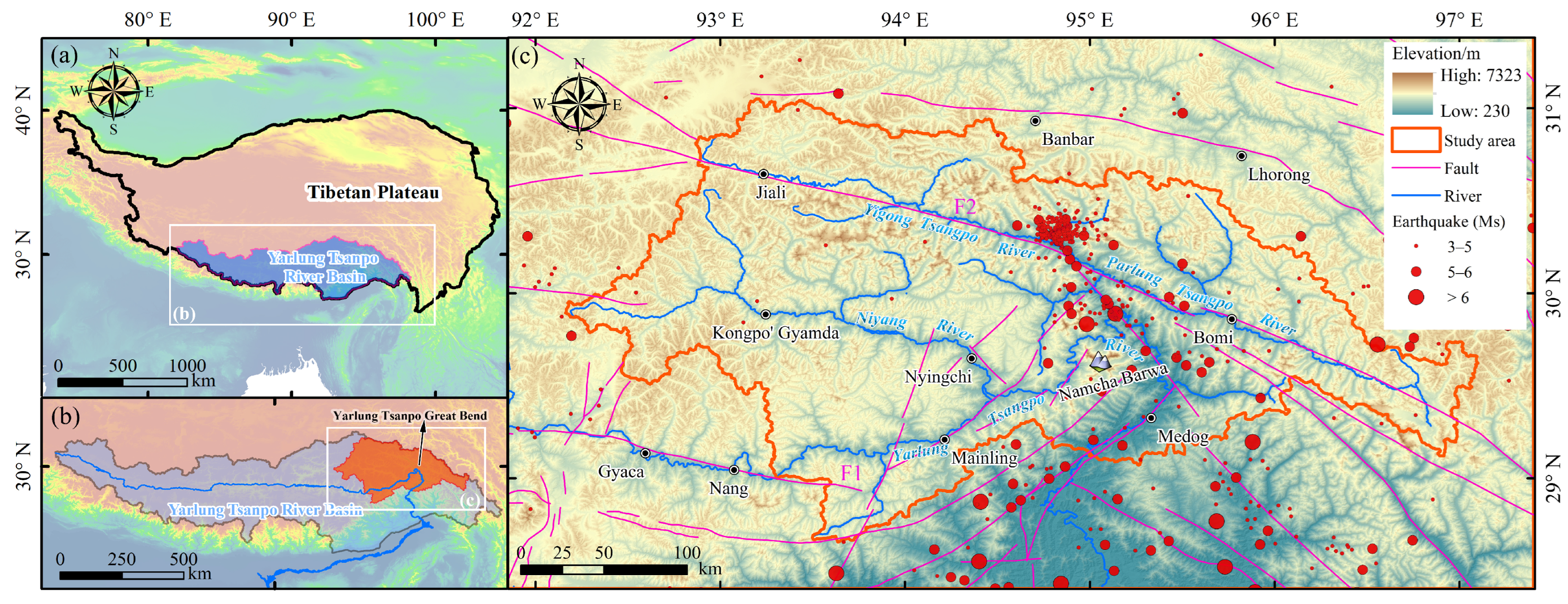
The study area is located in the southeastern part of the Tibetan Plateau, within the Yarlung Tsangpo River Basin (Figure 1a), near the Yarlung Tsangpo Grand Bend (Figure 1b). It covers the adjacent tributary basins, including the Parlung Tsangpo, Yigong Tsangpo, and the confluence area of the Niyang River and Yarlung Tsangpo (Figure 1c), within the geographical coordinates of 92.162°E to 97.1°E and 28.655°N to 31.05°N, covering a total area of approximately 63,275 km². The Yarlung Tsangpo River flows from west to east into the study area, receiving major tributaries such as the Niyang River and Parlung Tsangpo, and after bending near Mount Namcha Barwa, finally exits the study area, flowing southwest through Meto. The topography of the study region generally shows a trend of higher elevation in the north and lower elevation in the south, with an average altitude of over 4000 m. The area is predominantly composed of high mountain canyons and high to extreme mountain landscapes. The terrain is highly variable, with intense surface incision. In the core eastern tectonic zone, river gradients can exceed 2000 m [41]. Warm and humid air currents from the Indian Ocean bring substantial moisture into the region along the Yarlung Tsangpo Grand Canyon [42], contributing to the extensive development of maritime glaciers in the high mountains.

Geologically, the study area is located near the core of the collision zone between the Indian Plate and the Eurasian Plate, close to the eastern tectonic zone. The area is characterized by strong tectonic deformation and hosts major deep faults, such as the Yarlung Tsangpo Fault Zone (F1) and the Jiali Fault (F2) [43]. The dominant tectonic features include thrusting, compression, and strike-slip [44]. The region has complex stratigraphy and lithology [45,46], with exposures of low to medium-grade metamorphic sedimentary rocks, granite belts, layered gneiss segments, and the Gangdise pluton. Intense tectonic activity has led to frequent seismic events in the region [36]. Coupled with complex topography and hydrodynamic conditions, the area is prone to geological hazards and frequent geological disasters [16,47,48,49], making it highly susceptible to large-scale river-blocking disasters [50]. Furthermore, the scale of engineering construction in the region is rapidly increasing, particularly in transportation infrastructure and hydropower projects, leading to the formation of numerous unstable slopes.

Figure 1. Overview map of the study area. (a) Regional location in southeastern Tibet; (b) Location of the study area in Yarlung Tsanpo River Basin; (c) Elevation map of the study area, with major rivers, faults, and historical earthquakes superimposed. The major faults are from Wu et al. [51], and the earthquakes with M > 3.0 up to 2020 were compiled from the USGS earthquake catalog (https://earthquake.usgs.gov/earthquakes/map/ (accessed on 24 July 2025)).

Figure 1. Overview map of the study area. (a) Regional location in southeastern Tibet; (b) Location of the study area in Yarlung Tsanpo River Basin; (c) Elevation map of the study area, with major rivers, faults, and historical earthquakes superimposed. The major faults are from Wu et al. [51], and the earthquakes with M > 3.0 up to 2020 were compiled from the USGS earthquake catalog (https://earthquake.usgs.gov/earthquakes/map/ (accessed on 24 July 2025)).

2.2. Materials

2.2.1. Landslide Inventory

This study integrates multi-source high-resolution optical imagery for landslide identification and boundary delineation. The landslide inventory for 1991–2020 was primarily compiled through visual interpretation of multi-temporal historical imagery available in Google Earth. This platform provides near-vertical, high-resolution imagery with local spatial resolutions finer than 0.5 m, facilitating the reliable detection of small landslides [52,53,54]. In addition, the 30 m Landsat historical archive, incorporated in Google Earth since 1984, supports the identification of long-term surface changes and enables approximate dating of landslide occurrences [55,56]. Images with low cloud cover, high visual quality, and acquisition dates close to the target periods were preferentially selected for landslide interpretation, boundary delineation, and activity-state assessment. For recent years with insufficient or unclear Google Earth imagery, supplementary verification was conducted using 21AT high-resolution satellite imagery accessed via OvitalMap V10.4.0 (Beijing Ovital Software Co., Ltd., Beijing, China), UAV images, and field photographs collected at 29 roadside sites. The data sources, spatial resolutions, and temporal coverage of each dataset are summarized in

Table 1. Data Sources and details.

Data	Resolution and Scale	Period	Source
Imagery	0.5–30 m	1991–2020	Google Earth https://www.google.cn/intl/zh-CN/earth/ (accessed on 22 November 2025)
Satellite imagery	0.3–2.0 m	2017–2020	21AT imagery accessed via OvitalMap V10.4.0 (Beijing Ovital Software Co., Ltd., Beijing, China)
DEM	30 m	—	ASTER GDEM v3, GDC http://www.gscloud.cn/ (accessed on 21 October 2024)
Stratigraphical lithology	1:500,000	—	National Tibetan Plateau Data Center https://data.tpdc.ac.cn/ (accessed on 26 December 2024)
Faults	1:4,000,000	—	Wu et al. [51]
River	1:1,000,000	—	National Catalogue Service for Geographic Information https://www.webmap.cn/ (accessed on 24 July 2025)
Precipitation	1 km	1991–2020	National Tibetan Plateau Data Center https://data.tpdc.ac.cn/ (accessed on 1 July 2025)
NDVI	250 m	1991–2020	Li et al. [57]
Earthquake	/	1991–2020	U.S. Geological Survey https://earthquake.usgs.gov/earthquakes/map/ (accessed on 24 July 2025)
Roads	1:1,000,000	2000, 2010, 2020	Gao and Sun [58] for 2000 and 2010; National Catalogue Service for Geographic Information for 2020 https://www.webmap.cn/ (accessed on 24 July 2025)

.

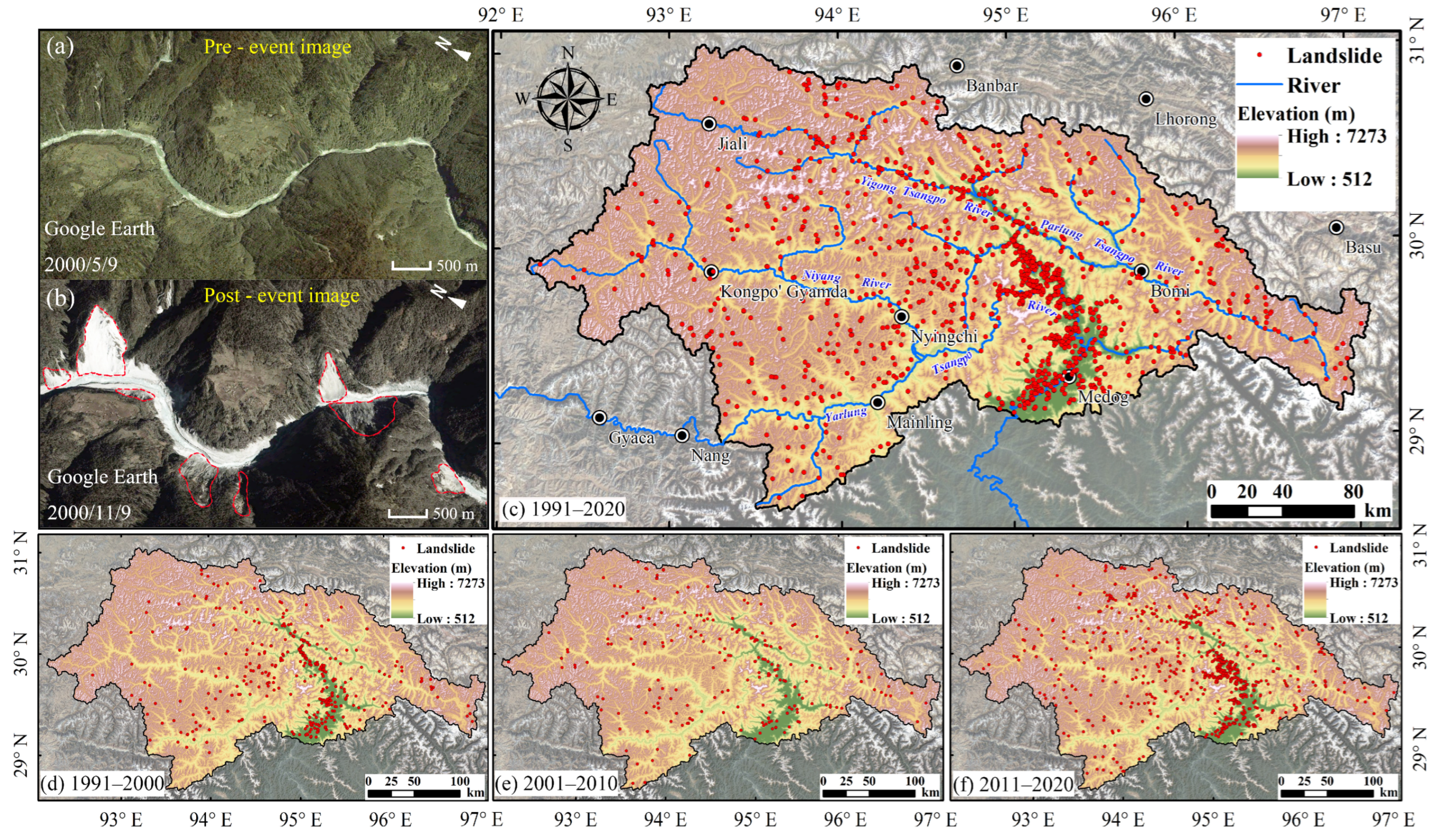
This study focuses on landslides larger than 104 m², which typically display distinct geomorphic signatures in high-resolution optical imagery and can significantly influence local landform evolution [59]. Landslide mapping was conducted based on multiple complementary criteria: (1) Morphological features, including scarps, fissures, runout traces, and exposed deposits [60]; (2) Vegetation anomalies, such as bare patches, vegetation gaps, and abnormal regrowth patterns [61]; (3) tonal or spectral contrasts between fresh bare rock, exposed soil, depositional zones, and surrounding stable slopes [62]. The mapped landslides were cross-checked using multi-source remote-sensing images, UAV observations, and field investigations where available, and the results were manually reviewed to reduce omission and misclassification. Each landslide polygon was further converted into an internal representative point in ArcGIS 10.8 (Esri, Redlands, CA, USA) for factor extraction and model training. The timing of landslide occurrences was constrained by comparison of pre- and post-event imagery, with each landslide assigned to the earliest year in which it could be reliably detected at annual resolution (Figure 2a,b).

A total of 1350 landslides were documented in the study area from 1991 to 2020 (Figure 2c). Following the classification scheme of [63], these landslides primarily comprise falls, slides, and flow-like types. To balance temporal resolution, inventory reliability, and sample-size requirements for period-specific modeling, a decadal time scale was adopted. The inventory was divided into three decadal periods: P1 (1991–2000), P2 (2001–2010), and P3 (2011–2020), containing 359, 217, and 774 landslides, respectively (Figure 2d–f). The landslides exhibit pronounced spatial heterogeneity across the study area, with high concentrations along the Yarlung Tsangpo Grand Canyon, the Parlung Tsangpo–Yigong Tsangpo valley system, and adjacent steep slopes, consistent with previous observations. During P1 (Figure 2d), landslides were predominantly concentrated along the middle to lower sections of the main valley corridors. In P2 (Figure 2e), landslide occurrences were more widely dispersed throughout the drainage network. By P3 (Figure 2f), the total number of landslides increased substantially, with clear clustering observed near the confluence of the Yarlung Tsangpo and Parlung Tsangpo rivers and on adjacent canyon slopes. Collectively, these observations indicate distinct spatiotemporal variations in landslide activity, characterized by shifts in both the intensity and spatial concentration of landslides from P1 to P3.

2.2.2. Landslide Conditioning Factors

Landslide initiation is controlled by multiple conditioning factors, but their selection in susceptibility assessment has not been fully standardized [64]. Nevertheless, topographic, geological, hydrological, climatic, land-cover, seismic, and anthropogenic factors are commonly used to characterize landslide-prone environments [65,66,67]. Based on previous studies and the environmental characteristics of the study area, this study constructed a multi-source conditioning factor system, including both static and dynamic factors. Static factors represent relatively stable topographic–geomorphic conditions, lithology, and proximity to faults and drainage networks, whereas dynamic factors describe period-specific variations in precipitation, vegetation cover, road proximity, and seismic disturbance. All factors were projected to the same coordinate system and resampled to a spatial resolution of 30 m × 30 m to ensure consistency among periods. The sources, spatial resolution, time range, and main applications of each data type are shown in Table 1.

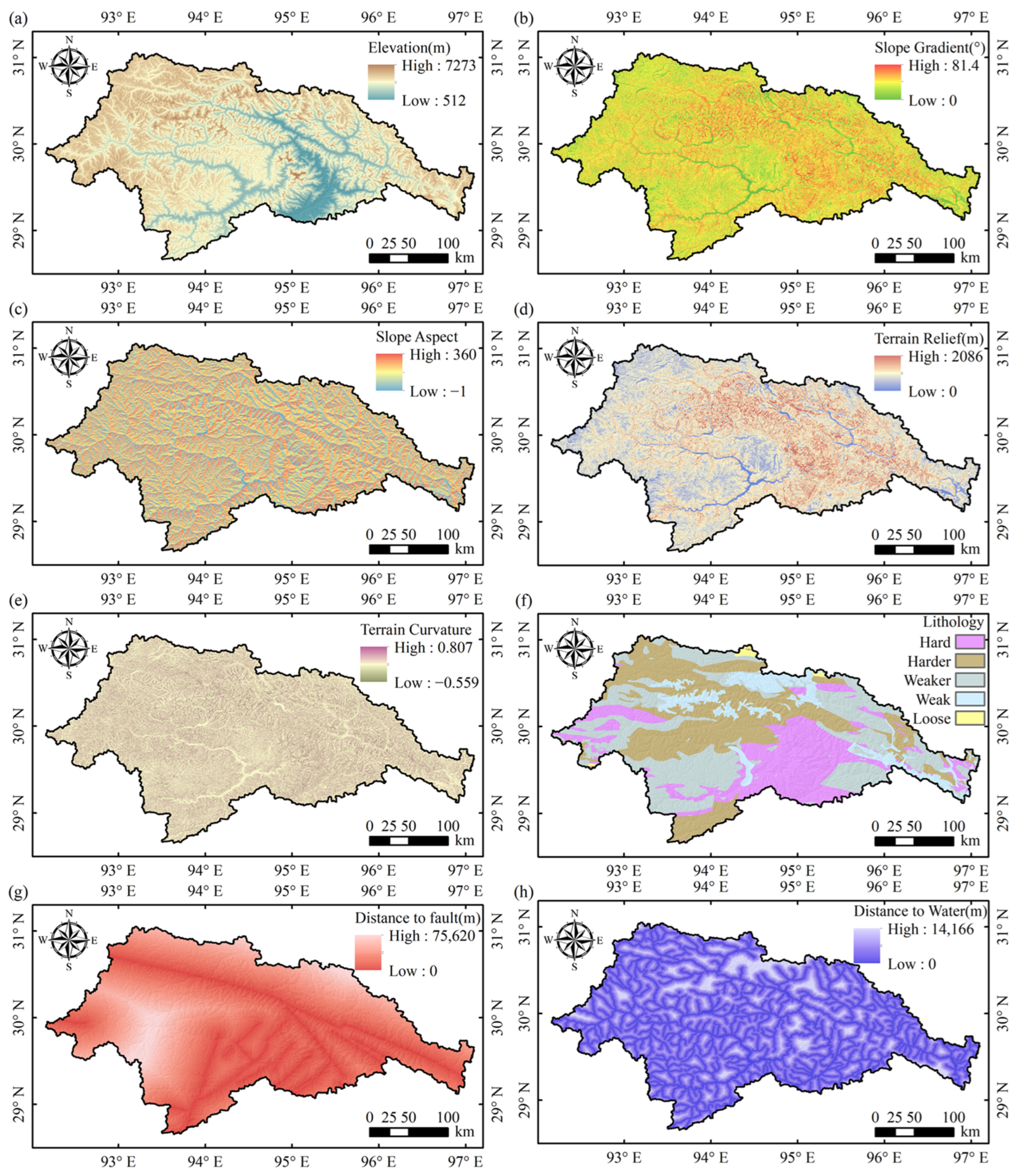
The static factors included elevation (ELE), slope gradient (SD), slope aspect (SA), terrain relief (TR), terrain curvature (TC), lithology (LT), distance to faults (DTF), and distance to water (DTW) (Figure 3). Topographic factors, including ELE, SD, SA, TR, and TC, were derived from the 30 m ASTER GDEM v3 accessed through the Geospatial Data Cloud (GDC). LT data was obtained from the lithological dataset provided by Qi [68] and accessed through the National Tibetan Plateau Data Center (TPDC). DTF and DTW were calculated using Euclidean distance analysis based on fault vector data from Wu et al. [51] and drainage vector data from the National Catalogue Service for Geographic Information (NCSGI), respectively, to represent tectonic and river-proximity effects. Together, these factors define the relatively stable geomorphic and geological background of landslide susceptibility.

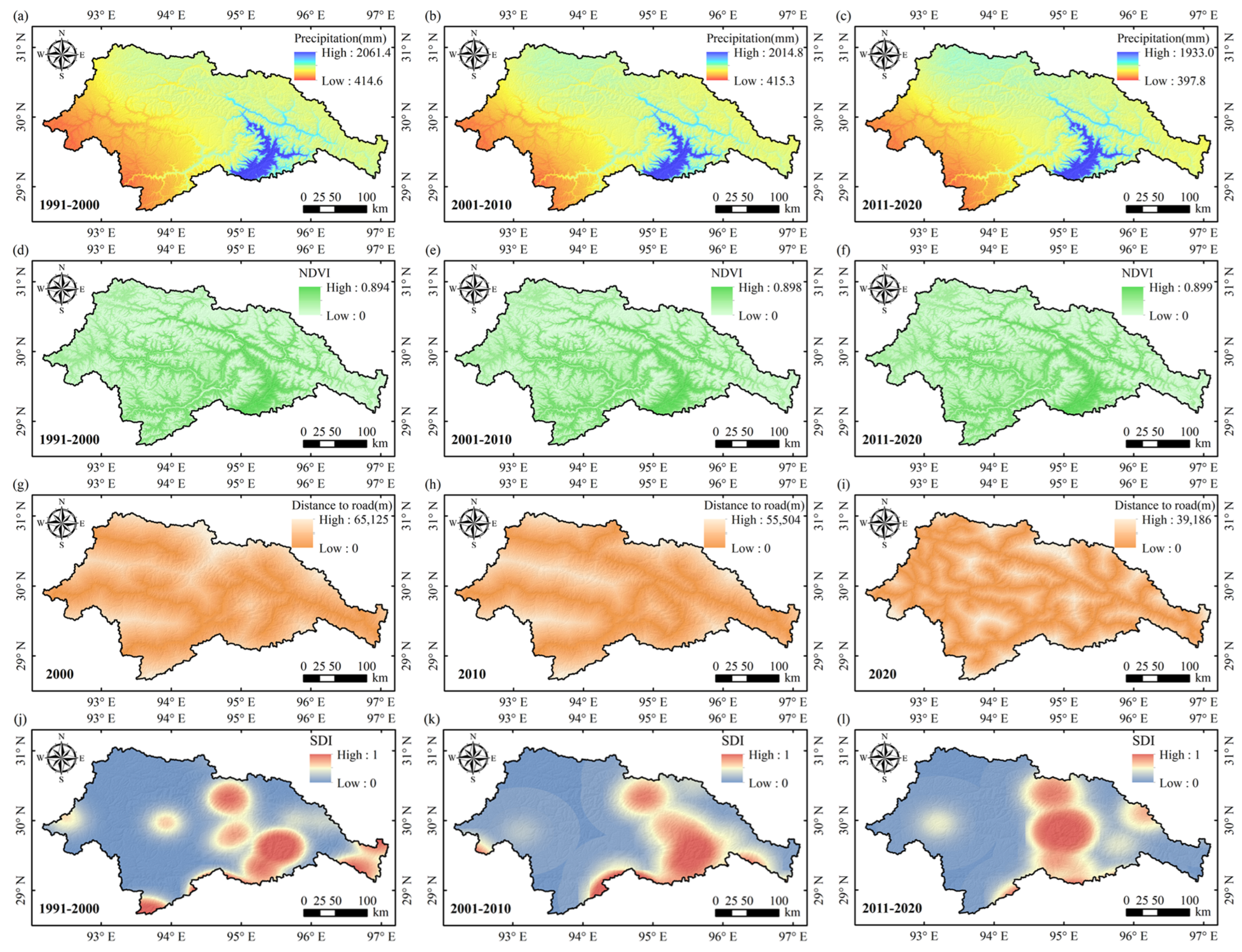
The dynamic factors included annual precipitation (AP), normalized difference vegetation index (NDVI), distance to roads (DTR), and a seismic disturbance proxy index, denoted as SDI in this study (Figure 4). The precipitation (AP) factor was derived from the monthly precipitation dataset developed by Peng et al. [69] and updated by Peng [70], accessed through the National Tibetan Plateau Data Center (TPDC). The NDVI factor was obtained from the 250 m monthly NDVI dataset provided by Li et al. [57]. Period-specific averages of AP and NDVI were calculated to represent hydroclimatic conditions and vegetation-cover variations, respectively. DTR was calculated from road network data for 2000, 2010, and 2020. The 2000 and 2010 datasets were obtained from Gao and Sun [58], whereas the 2020 dataset was supplemented from NCSGI. Roads below Class IV in the NCSGI dataset were excluded to improve consistency, and all datasets were processed using the same projection, raster resolution, and Euclidean distance calculation. As gridded measured PGA data suitable for multi-temporal comparison were unavailable for the study area, a PGA-like seismic disturbance proxy was constructed from U.S. Geological Survey earthquake catalogue data (USGS). The proxy integrated epicentral location, magnitude, distance attenuation, and temporal weighting following the spatial logic of the USGS ShakeMap methodology [71,72,73], and is hereafter referred to as SDI. To reduce boundary effects, earthquakes within the study area and a 100 km buffer around its boundary were included in the calculation. It should be noted that SDI in this study does not represent observed peak ground acceleration, but rather a period-specific proxy used to describe relative spatial differences in seismic disturbance among periods. These dynamic factors were used to capture stage-dependent environmental and anthropogenic variations that may affect local landslide susceptibility.

2.3. Methods

2.3.1. Framework in This Study

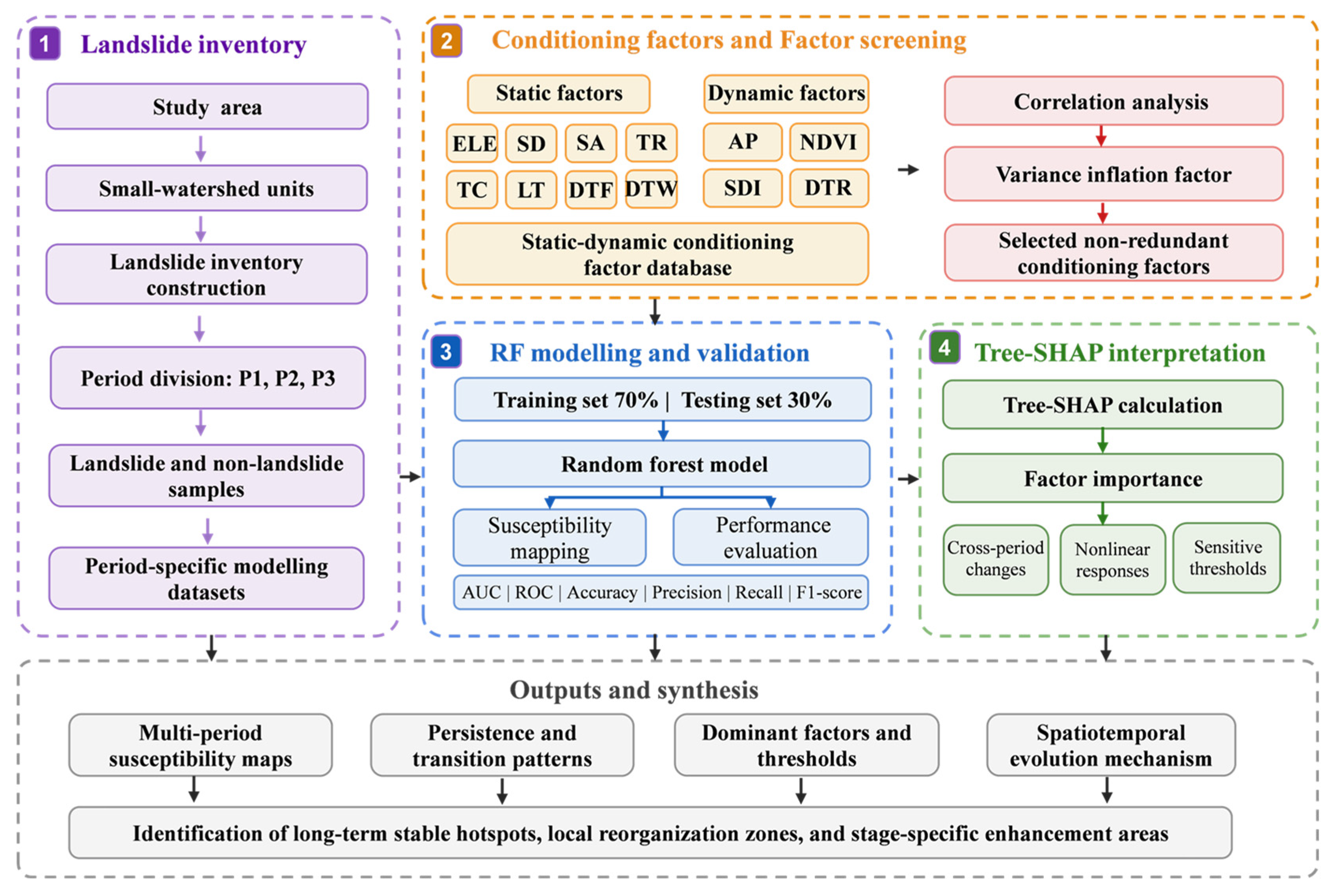
This study constructed multi-temporal landslide inventories and conditioning factor datasets, and evaluated landslide susceptibility while revealing its spatiotemporal evolution characteristics using random forest and Tree-SHAP interpretation. Figure 5 shows the flowchart of the process. The key steps mainly include the following aspects:

(1)

The landslide spatiotemporal distribution inventory was constructed based on long-term high-resolution historical optical imagery and field survey data, with temporal segmentation into distinct periods.

(2)

A static and dynamic conditioning factor system was constructed, and redundant factors were removed using correlation analysis and variance inflation factor (VIF) testing.

(3)

Period-specific modeling datasets were established, random forest models were trained for each period, landslide susceptibility zoning maps were generated and model performance and mapping reliability were evaluated.

(4)

Tree-SHAP was used to interpret stage-dependent changes in the dominant factors from three perspectives: factor importance, cross-period contribution variations, and nonlinear response relationships.

Random Forest modeling, model performance evaluation, and SHAP-based interpretation were implemented in Python 3.11.14 under the Anaconda environment (Anaconda, Inc., Austin, TX, USA). The Random Forest models were implemented using scikit-learn 1.7.1, and SHAP values were calculated using SHAP 0.50.0.

2.3.2. Conditioning Factor Screening

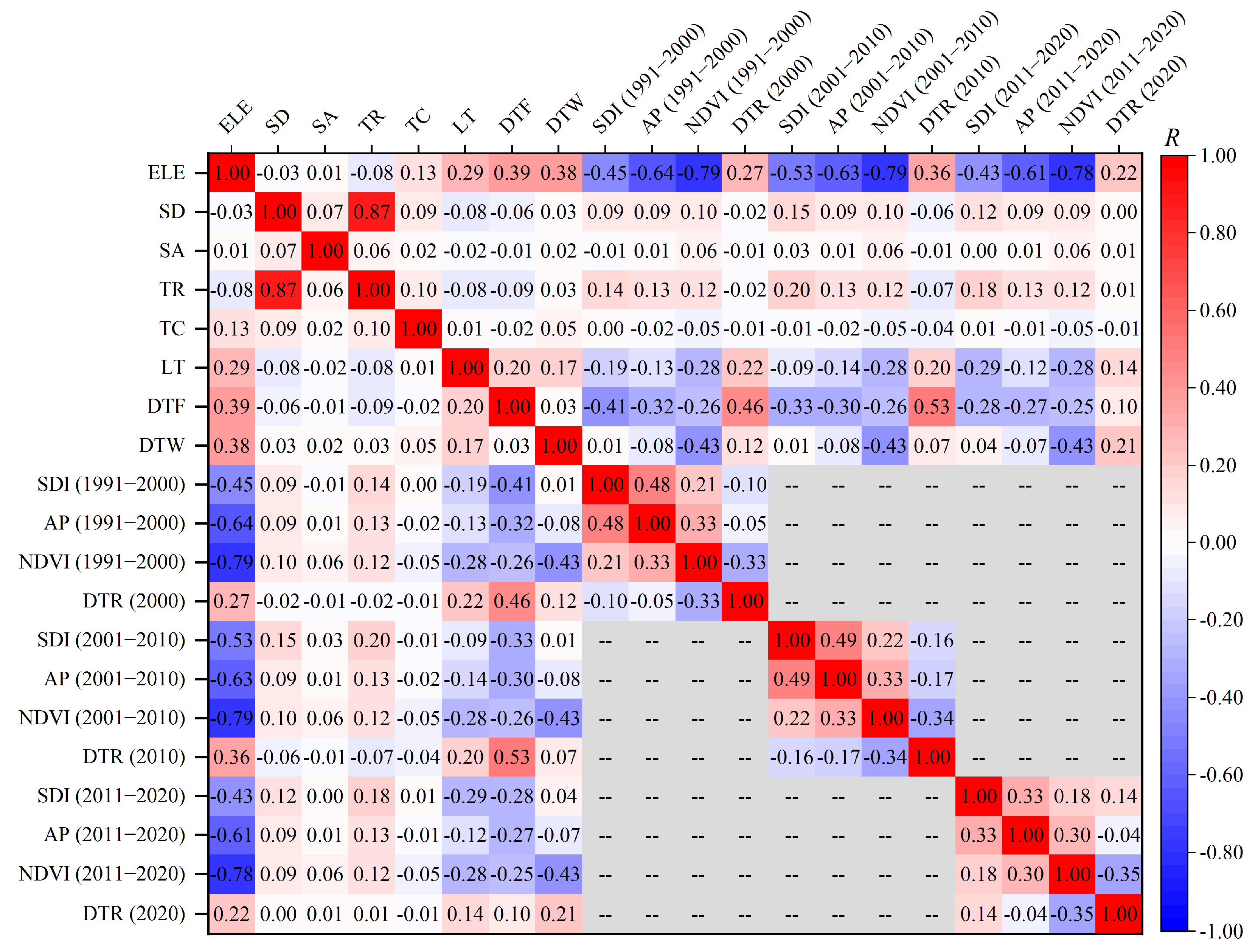
Before model training, correlation analysis and multicollinearity testing were performed on the conditioning factors to reduce redundancy and improve the robustness and comparability of model interpretation among periods. Multicollinearity was assessed using the variance inflation factor (VIF) and tolerance (TOL), where VIF > 10 or TOL < 0.1 indicates severe collinearity and suggests that the corresponding factor should be removed [74,75]. Pairwise linear correlations among factors were evaluated using the absolute Pearson correlation coefficient |R|. Following previous studies, |R| < 0.3 was considered negligible correlation, 0.3 ≤ |R| < 0.5 low correlation, 0.5 ≤ |R| < 0.8 moderate correlation, and |R| ≥ 0.8 high correlation [38]. The multicollinearity results (

Table 2. Variance Inflation Factor (VIF) and Tolerance (TOL) of the conditioning factors.

Factor	P1 (1991–2000)		P2 (2001–2010)		P3 (2011–2020)
	VIF	TOL	VIF	TOL	VIF	TOL
ELE	5.967	0.168	6.866	0.146	5.855	0.171
SD	4.260	0.235	4.264	0.235	4.259	0.235
SA	1.022	0.979	1.025	0.976	1.022	0.978
TC	1.058	0.945	1.062	0.941	1.060	0.944
LT	1.145	0.873	1.130	0.885	1.196	0.836
DTF	1.604	0.624	1.584	0.632	1.246	0.803
DTW	1.316	0.760	1.343	0.745	1.345	0.743
SDI	1.574	0.635	1.836	0.545	1.579	0.633
AP	2.219	0.451	2.055	0.487	1.919	0.521
NDVI	3.652	0.274	3.790	0.264	3.578	0.279
DTR	1.423	0.703	1.525	0.656	1.222	0.818

) show that all factors in the three period-specific factor sets had TOL values greater than 0.1 and VIF values lower than 10, indicating no severe multicollinearity. The correlation matrix (Figure 6) further shows a high correlation between slope gradient and topographic relief, with |R| ≥ 0.8. Because both factors describe terrain steepness, topographic relief was excluded, whereas slope gradient was retained as the more representative factor. The final factor set included 11 factors: ELE, SD, SA, TC, LT, DTF, DTW, AP, NDVI, SDI, and DTR, which were used for period-specific database construction and random forest model training.

2.3.3. Database Construction

Before conducting period-specific landslide susceptibility modelling, it is essential to construct landslide/non-landslide sample databases in advance. Independent landslide/non-landslide sample datasets were constructed for P1 (1991–2000), P2 (2001–2010), and P3 (2011–2020) respectively. The 359, 217, and 774 inventoried landslides in P1, P2, and P3, respectively, were used as positive samples (class 1). Correspondingly, non-landslide candidate areas were defined as areas outside the mapped landslide polygons, and areas with slope gradients <5° were also regarded as non-landslide areas following previous studies [76]. From these candidate areas, an equal number of non-landslide points were randomly generated as negative samples (class 0), with a minimum spacing of 500 m between non-landslide points to reduce spatial clustering [77]. Given the low density of P3 negative samples, approximately 0.012 samples km⁻², this spacing mainly reduced local redundancy without strongly constraining their regional distribution. Raster values of the selected conditioning factors were extracted at landslide and non-landslide sample locations to build period-specific modelling datasets. Static factors were shared across periods, whereas dynamic factors were extracted separately for each period. Each dataset was split into training and testing subsets at a ratio of 70:30 [78]. The training set (70%) was used for random forest model training, and the testing set (30%) was used for model performance validation.

2.3.4. Random Forest Model

Random forest model (RF) is a non-parametric ensemble learning method proposed by [19]. It constructs multiple decision trees using bootstrap samples and random subsets of predictor variables, and combines their outputs to improve prediction accuracy and robustness. Owing to its ability to handle high-dimensional data, nonlinear relationships, and complex variable interactions, RF has been widely used in landslide susceptibility assessment [79,80,81]. In this study, independent RF models were trained for P1, P2, and P3 using the selected conditioning factors as predictors and the landslide/non-landslide labels as the binary response variable. The predicted probability of each grid cell belonging to the landslide class was used as the landslide susceptibility index for subsequent mapping and classification.

To ensure comparability among periods, the same parameter settings were applied to the three RF models. The number of trees was set to 500 (n_estimators = 500), and tree depth was not limited (max_depth = None). The options class_weight = “balanced” and random_state = 42 were used to improve robustness and reproducibility, while n_jobs = −1 was adopted for parallel computation. Other parameters were kept at their default values.

2.3.5. SHAP-Based Explainability

To interpret the relative importance and cross-period variations in conditioning factors in the period-specific random forest models, the Tree-SHAP method was applied to explain model outputs. Tree-SHAP is an efficient implementation of SHAP values for tree-based models and is grounded in Shapley value theory, which allocates a model prediction among input features according to their marginal contributions [26,82]. For a given sample, the prediction of the RF model can be decomposed into the expected model output and the sum of feature-specific SHAP values. Thus, the SHAP value of each feature quantifies its contribution to increasing or decreasing the predicted landslide susceptibility relative to the baseline prediction [83]. For any given sample x, the model output can be expressed as:

$$f\left(x\right)={\varnothing }_0+{\displaystyle \sum _{i=1}^M}{\varnothing }_i$$

(1)

where f(x) is the predicted output of the model for sample x, ϕ₀ is the expected model output or baseline value, M is the number of input features, and ϕ_i is the SHAP value of the i-th feature:

$${\varnothing }_i=\sum _{S\subseteq F\backslash i}{\displaystyle \frac{\left|S\right|!\left(M-\left|S\right|-1\right)!}{M!}}\left[f\left(S\cup \left\{i\right\}\right)-f\left(S\right)\right]$$

(2)

where F is the set of all input features, M is the number of features, and S is any feature subset excluding the i-th feature. f(S) and f(S∪{i}) represent the model outputs without and with the i-th feature, respectively. The SHAP value ϕ_i therefore quantifies the average marginal contribution of feature i to the model prediction across all possible feature subsets.

2.3.6. Model Performance Evaluation

To assess the reliability of the period-specific landslide susceptibility models, model performance was evaluated using confusion matrix-based metrics and receiver operating characteristic (ROC) curves. The confusion matrix metrics included accuracy, precision, recall, and F1-score, which were used to evaluate overall classification performance, the reliability of landslide predictions, the ability to correctly identify landslide samples, and the balance between precision and recall, respectively. The formulas are given as follows:

$$\mathrm{A}\mathrm{c}\mathrm{c}\mathrm{u}\mathrm{r}\mathrm{a}\mathrm{c}\mathrm{y}={\displaystyle \frac{TP+TN}{TP+TN+FP+FN}}$$

(3)

$$\mathrm{P}\mathrm{r}\mathrm{e}\mathrm{c}\mathrm{i}\mathrm{s}\mathrm{i}\mathrm{o}\mathrm{n}={\displaystyle \frac{TP}{TP+FP}}$$

(4)

$$\mathrm{R}\mathrm{e}\mathrm{c}\mathrm{a}\mathrm{l}\mathrm{l}={\displaystyle \frac{TP}{TP+FN}}$$

(5)

$$\mathrm{F}1\text{-}\mathrm{s}\mathrm{c}\mathrm{o}\mathrm{r}\mathrm{e}={\displaystyle \frac{2TP}{2TP+FN+FP}}$$

(6)

In the equation, TP and TN represent correctly classified landslide and non-landslide samples, respectively, whereas FP and FN denote non-landslide samples misclassified as landslides and landslide samples misclassified as non-landslides. Accuracy, precision, recall, and F1-score range from 0 to 1, with higher values indicating better classification performance.

ROC curves were further used to assess model discrimination ability [84,85,86]. The ROC curve plots the true positive rate (TPR) against the false positive rate (FPR) at different probability thresholds, and the area under the curve (AUC) quantifies the model’s ability to distinguish landslide from non-landslide samples. An AUC of 0.5 indicates random prediction, whereas values closer to 1.0 indicate stronger predictive performance [87].

3. Results

3.1. Model Performance

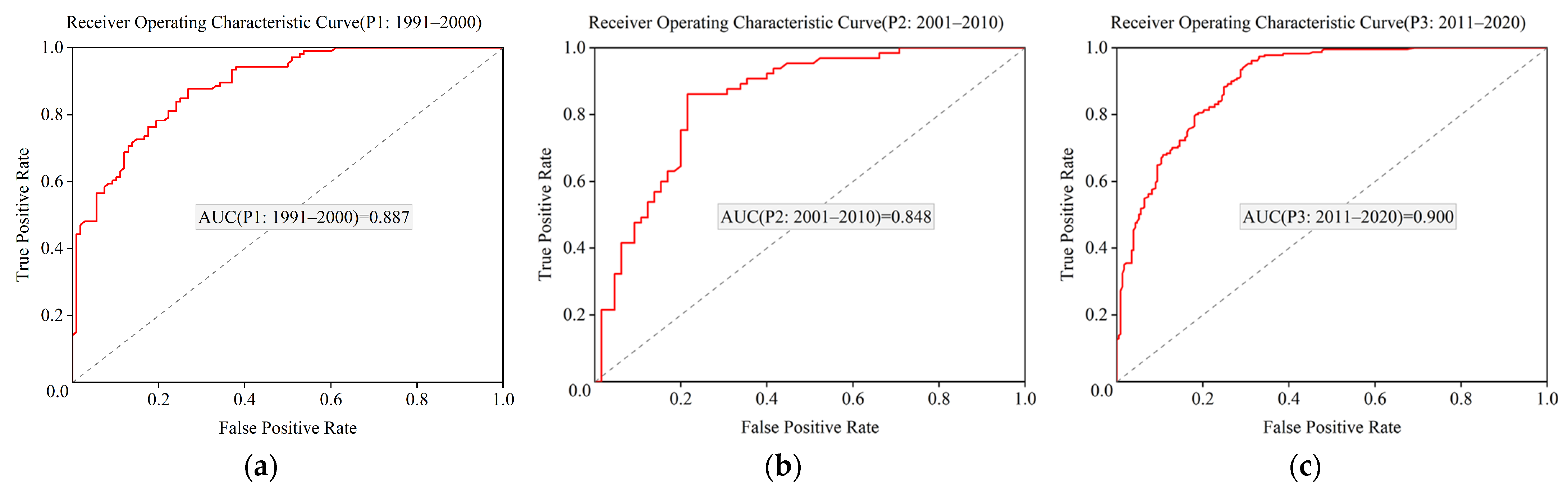
The predictive performance of the period-specific random forest models was evaluated using independent testing datasets for P1 (1991–2000), P2 (2001–2010), and P3 (2011–2020). Figure 7 presents the receiver operating characteristic (ROC) curves for the three periods. All curves were clearly above the random-classification baseline, with AUC values of 0.887, 0.848, and 0.900, respectively. These values all exceeded 0.80, indicating good discriminatory ability for landslide and non-landslide samples [25]. The relatively lower AUC in P2 may be related to the smaller number of mapped landslides and the limited positive samples available for testing. The accuracy, precision, recall, and F1-score values summarized in

Table 3. Performance of the period-specific RF models.

Period	Accuracy	Precision	Recall	F1-Score	AUC
P1 (1991–2000)	0.794	0.782	0.811	0.796	0.887
P2 (2001–2010)	0.823	0.800	0.862	0.830	0.848
P3 (2011–2020)	0.802	0.791	0.818	0.804	0.900

were also consistently high, with only limited inter-period variation. These results suggest that the period-specific RF models are sufficiently reliable for subsequent landslide susceptibility mapping and Tree-SHAP-based interpretation.

3.2. Multi-Temporal Landslide Susceptibility Mapping

3.2.1. Spatial Distribution of Susceptibility Classes

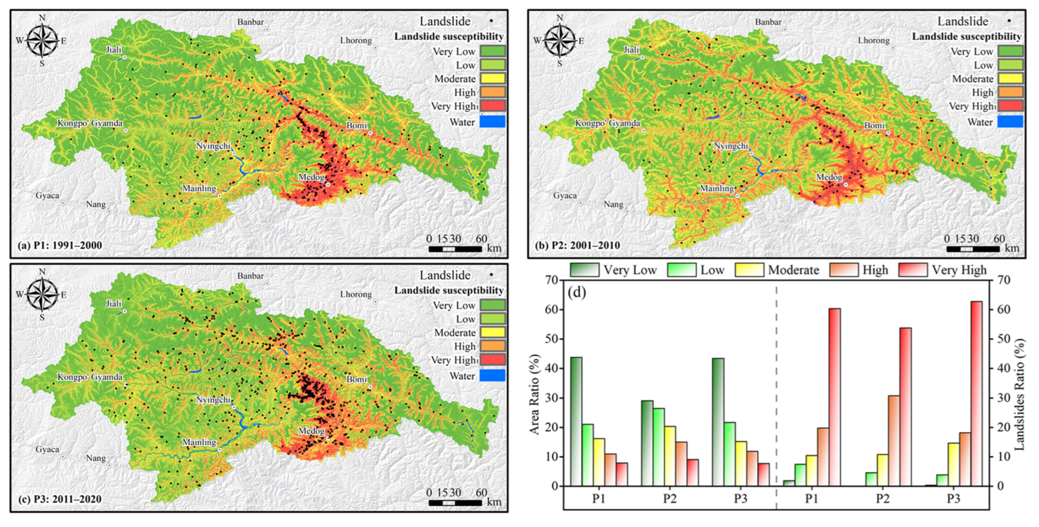
Period-specific random forest models were used to generate landslide susceptibility index (LSI) maps for P1, P2, and P3. The susceptibility index of each period was first classified into five classes using the Jenks natural breaks method. To ensure comparability among periods, the maximum breakpoint values among the three period-specific classifications were adopted as common thresholds. Accordingly, the LSI values were classified into five susceptibility classes: very low (0–0.161), low (0.161–0.321), moderate (0.321–0.498), high (0.498–0.710), and very high (0.710–1.000).

As shown in Figure 8a–c, the susceptibility maps show pronounced spatial heterogeneity but retain broadly consistent first-order spatial patterns across the three periods. High and very high susceptibility zones are mainly concentrated along the Yarlung Tsangpo–Parlung Tsangpo–Yigong Tsangpo river system and its major tributaries. Notable high-susceptibility clusters occur in the Yarlung Tsangpo Grand Canyon, the downstream valleys near Medog, the Parlung Tsangpo–Yigong Tsangpo segment, the Niyang River–Yarlung Tsangpo confluence, and deeply incised tributary junctions. In contrast, very low and low susceptibility zones are mainly distributed on high-elevation ridges, watershed divides, and relatively gentle slopes away from the main valley corridors. Despite this persistent spatial framework, the extent, continuity, and concentration of high-susceptibility zones varied among periods. In P1, high and very high susceptibility zones were mainly confined to the middle and lower reaches of the main valley corridors. In P2, these zones became more continuous along the drainage network and extended into major tributaries and downstream valleys, accompanied by an expansion of moderate susceptibility areas. In P3, high-susceptibility zones became more locally concentrated, particularly near the Yarlung Tsangpo–Parlung Tsangpo confluence, earthquake-affected valley sections, and major tributary junctions. These results indicate that the regional susceptibility pattern remained broadly stable, while local susceptibility levels underwent stage-dependent expansion, redistribution, and reconcentration.

The area ratio, landslide ratio, and landslide frequency ratio (FR) results support the validity of the susceptibility classification (

Table 4. Area ratio, landslide ratio, and frequency ratio of different susceptibility classes in the three periods.

Susceptibility Class	P1 (1991–2000)			P2 (2001–2010)			P3 (2011–2020)
	Area Ratio	Landslide Ratio	FR	Area Ratio	Landslide Ratio	FR	Area Ratio	Landslide Ratio	FR
Very low	43.8%	1.9%	0.04	29.1%	0.0%	0.00	43.5%	0.4%	0.01
Low	21.1%	7.5%	0.36	26.5%	4.6%	0.17	21.7%	3.9%	0.18
Moderate	16.2%	10.4%	0.64	20.3%	10.8%	0.53	15.2%	14.7%	0.97
High	11.0%	19.8%	1.80	15.0%	30.8%	2.05	11.9%	18.2%	1.53
Very High	7.9%	60.4%	7.65	9.1%	53.8%	5.91	7.7%	62.8%	8.16

and Figure 8d). FR was calculated as the landslide ratio divided by the area ratio for each susceptibility class. The very low and low classes occupied 64.9%, 55.6%, and 65.2% of the study area in P1, P2, and P3, respectively, but contained only 9.4%, 4.6%, and 4.3% of mapped landslides. Conversely, the high and very high classes covered only 18.9%, 24.1%, and 19.6% of the area, yet contained 80.2%, 84.6%, and 81.0% of landslides, respectively. The very high class alone accounted for only 7.7–9.1% of the area but contained 53.8–62.8% of landslides. FR values were below 1 in the very low to moderate classes and exceeded 1 in the high and very high classes, indicating that the classification effectively captures the spatial concentration of mapped landslides.

3.2.2. Temporal Transition in Susceptibility Classes

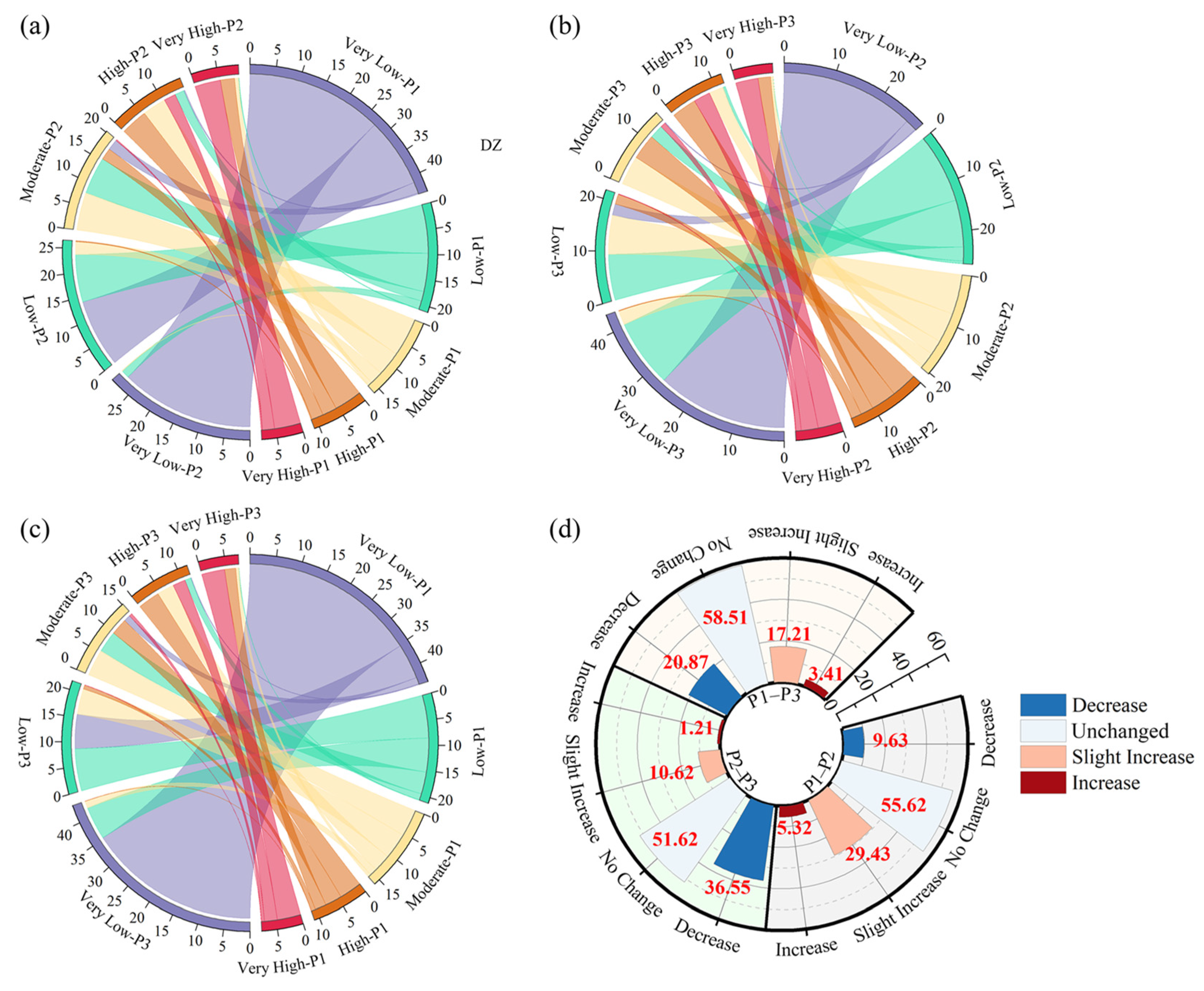
To examine temporal changes in landslide susceptibility, class transitions were analyzed for P1–P2, P2–P3, and P1–P3 using chord diagrams and transition statistics. Class transitions were grouped into decrease, unchanged, slight increase, and increase. As shown in Figure 9, unchanged areas dominated all three comparisons, indicating strong temporal continuity in the susceptibility pattern. Nevertheless, localized class changes occurred mainly along valley margins, susceptibility hotspots, and transitional zones between moderate and high susceptibility classes.

For P1–P2 (Figure 9a,d), unchanged areas accounted for 55.62% of the study area, whereas combined upward transitions, including slight increase and increase classes, accounted for 34.75%, and downward transitions accounted for 9.63%. The dominance of upward transitions indicates local susceptibility increases from P1 to P2, particularly around pre-existing high-susceptibility cores and adjacent valley corridors. For P2–P3 (Figure 9b,d), class transitions became more active and were dominated by downward shifts. Unchanged areas decreased to 51.62%, while downward transitions increased to 36.55%. Upward transitions accounted for 11.83% of the study area, including slight increase transitions of 10.62% and increase transitions of 1.21%. This pattern indicates partial downgrading or contraction of previously high-susceptibility zones, together with localized susceptibility increases in specific valley sections and tributary areas.

Over the full P1–P3 interval (Figure 9c,d), unchanged areas remained dominant, accounting for 58.51% of the study area. Downward and upward transitions accounted for 20.87% and 20.62%, respectively. Overall, the transition analysis indicates that the first-order susceptibility pattern remained broadly stable across the three decades, with Kappa coefficients of 0.416, 0.363, and 0.424 for P1–P2, P2–P3, and P1–P3, respectively, indicating that the observed spatial agreement exceeded chance-level agreement. Local susceptibility levels changed mainly along valley margins, tributary junctions, and pre-existing susceptibility hotspots.

3.3. SHAP-Based Interpretation

3.3.1. Global Importance of Conditioning Factors

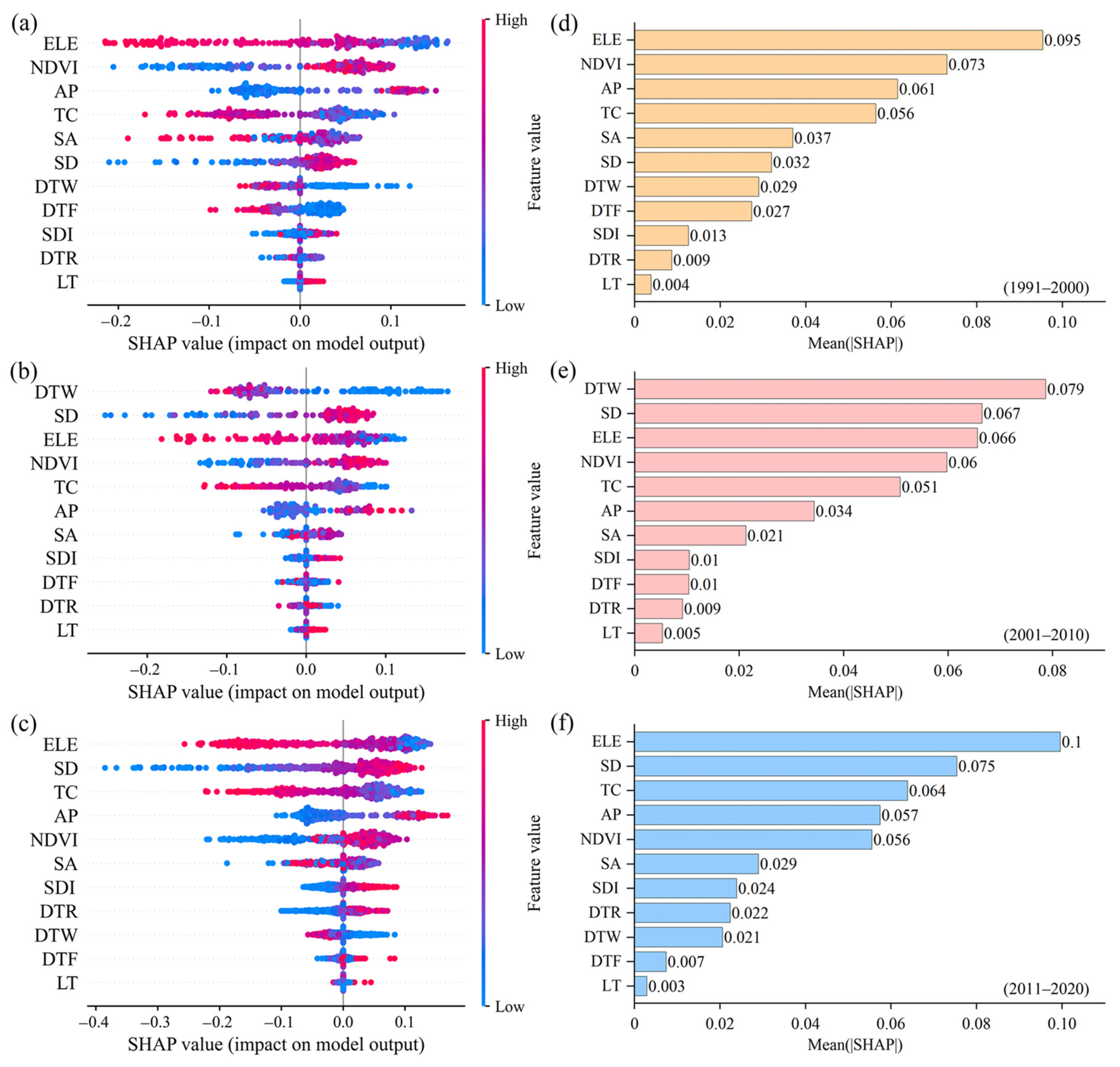
Tree-SHAP was applied to identify the dominant conditioning factors and interpret their contributions to period-specific RF predictions. SHAP values quantify the contribution of each factor to the model output at both global and local levels. Positive SHAP values indicate an increase in predicted landslide susceptibility, whereas negative values indicate a decreasing effect [88]. Global factor importance was quantified using the mean absolute SHAP value, Mean(|SHAP|), calculated across all samples within each period-specific RF model.

Figure 10 presents the SHAP-based global interpretation results for the three period-specific RF models. In the beeswarm plots (Figure 10a–c), the horizontal position represents the SHAP contribution to model output, whereas color indicates the original factor value. The asymmetric and widely dispersed SHAP distributions indicate heterogeneous and potentially nonlinear effects of conditioning factors on susceptibility predictions. The Mean(|SHAP|) rankings in Figure 10d–f show that the relative importance of individual factors differed among periods, although the dominant-factor structure remained broadly consistent. Elevation (ELE), slope gradient (SD), normalized difference vegetation index (NDVI), annual precipitation (AP), and terrain curvature (TC) consistently ranked among the leading factors. By contrast, distance to water (DTW), the seismic disturbance proxy (SDI), and road proximity (DTR) showed more pronounced temporal variability.

3.3.2. Temporal Shifts in Dominant Factor Composition

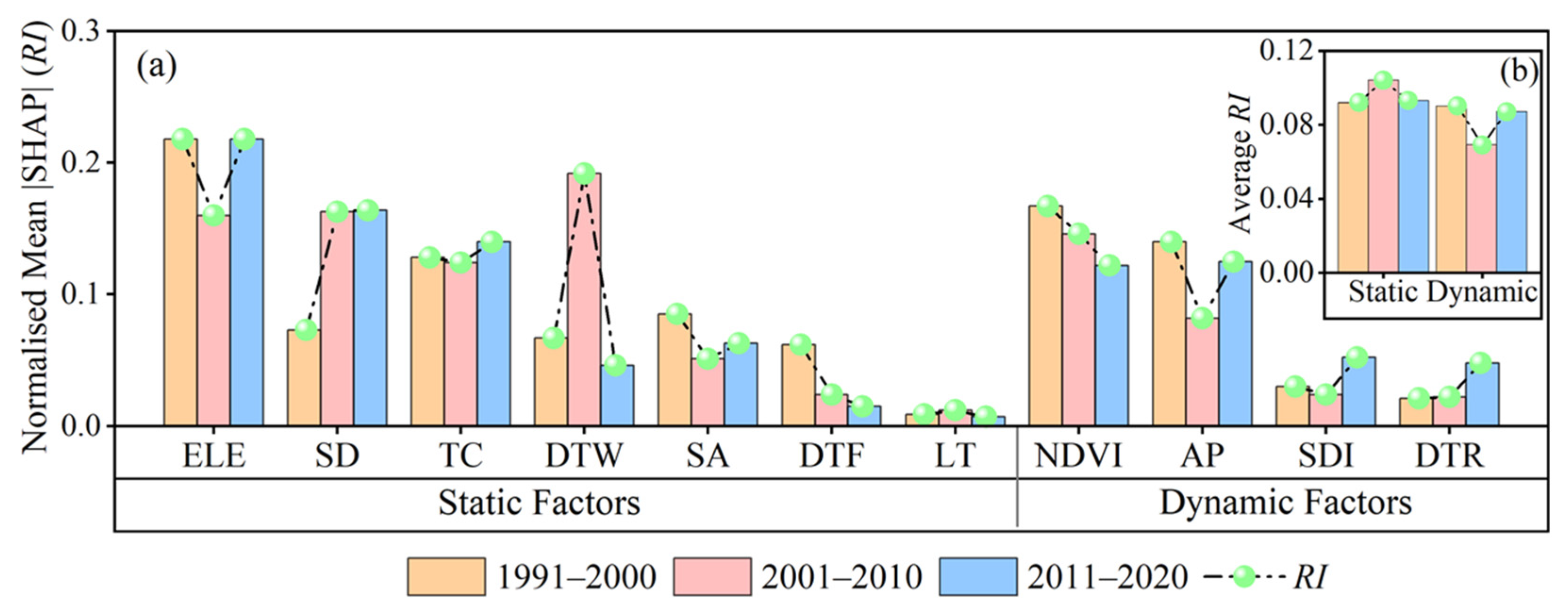
Because the three RF models were trained independently, raw Mean (|SHAP|) values are not directly comparable among periods. Mean (|SHAP|) values were therefore normalized within each period to obtain a relative importance index (RI) for cross-period comparison (

Table 5. Global importance and temporal changes in the relative importance index (RI) of conditioning factors across the three periods. RI denotes the normalized Mean (|SHAP|) value within each period. S/D denotes static/dynamic factors.

Factor	Type (S/D)	P1 (1991–2000)		P2 (2001–2010)		P3 (2011–2020)
		Mean (|SHAP|)	RI	Mean (|SHAP|)	RI	Mean (|SHAP|)	RI
ELE	S	0.095	0.218	0.066	0.160	0.100	0.218
SD	S	0.032	0.073	0.067	0.163	0.075	0.164
SA	S	0.037	0.085	0.021	0.051	0.029	0.063
TC	S	0.056	0.128	0.051	0.124	0.064	0.140
LT	S	0.004	0.009	0.005	0.012	0.003	0.007
DTF	S	0.027	0.062	0.010	0.024	0.007	0.015
DTW	S	0.029	0.067	0.079	0.192	0.021	0.046
SDI	D	0.013	0.030	0.010	0.024	0.024	0.052
AP	D	0.061	0.140	0.034	0.082	0.057	0.125
NDVI	D	0.073	0.167	0.060	0.146	0.056	0.122
DTR	D	0.009	0.021	0.009	0.022	0.022	0.048

). RI reflects the relative contribution of each factor within a period-specific model and should be interpreted as a model-derived comparative metric rather than an absolute physical contribution.

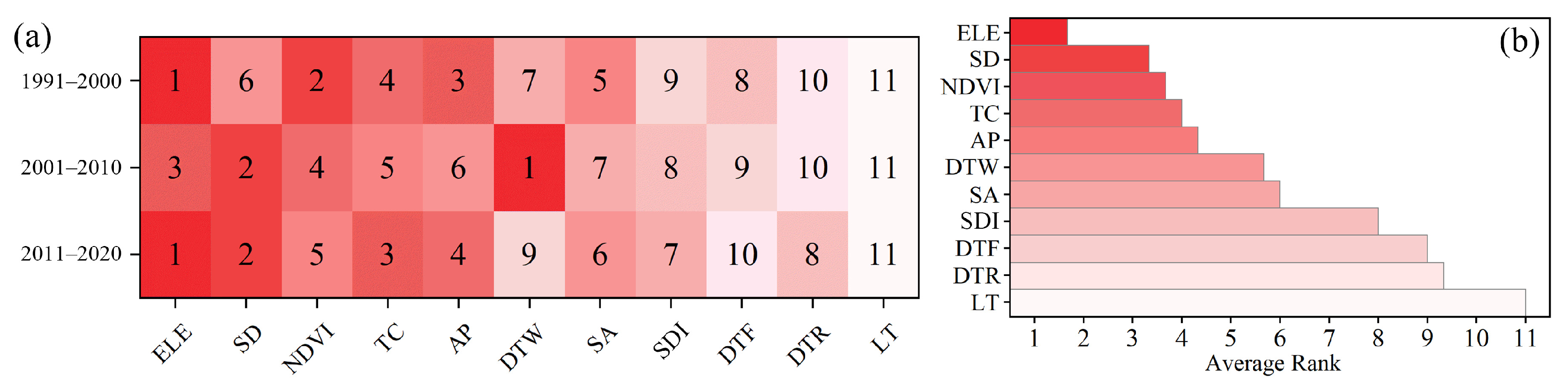
Figure 11a shows the cross-period RI changes in individual conditioning factors. ELE and TC maintained relatively high and stable RI values across the three periods, indicating persistent contributions from topographic and geomorphic conditions. SD increased from P1 to P2 and remained relatively stable in P3, whereas DTW showed the strongest fluctuation, reaching its highest RI in P2 and declining in P3. Slope aspect (SA) remained a secondary but non-negligible static factor, while distance to faults (DTF) and lithology (LT) consistently showed weak contributions and did not substantially alter the dominant-factor structure. Among the dynamic or time-varying factors, NDVI remained consistently important, while AP also ranked among the leading factors despite moderate RI fluctuations. In contrast, the seismic disturbance proxy and road proximity increased markedly in P3, indicating enhanced model contributions of earthquake-related and road-related factors during the later period. Figure 11b further shows that, after normalization by the number of factors, static factors had slightly higher average RI values than dynamic factors in P1, P2, and P3, with values of 0.092 versus 0.090, 0.104 versus 0.069, and 0.093 versus 0.087, respectively.

Figure 12 confirms this pattern from the perspectives of factor ranking and cumulative RI. ELE, SD, NDVI, TC, and AP consistently ranked among the leading factors, whereas DTW rose to first place in P2 before declining in P3. The cumulative RI of the top six factors reached 81.1%, 86.7%, and 83.2% in P1, P2, and P3, respectively. These results indicate that the dominant-factor system remained broadly stable across periods, while DTW in P2 and the seismic disturbance proxy and road proximity in P3 showed clear stage-dependent adjustments.

3.3.3. Nonlinear Responses of Dominant Factors

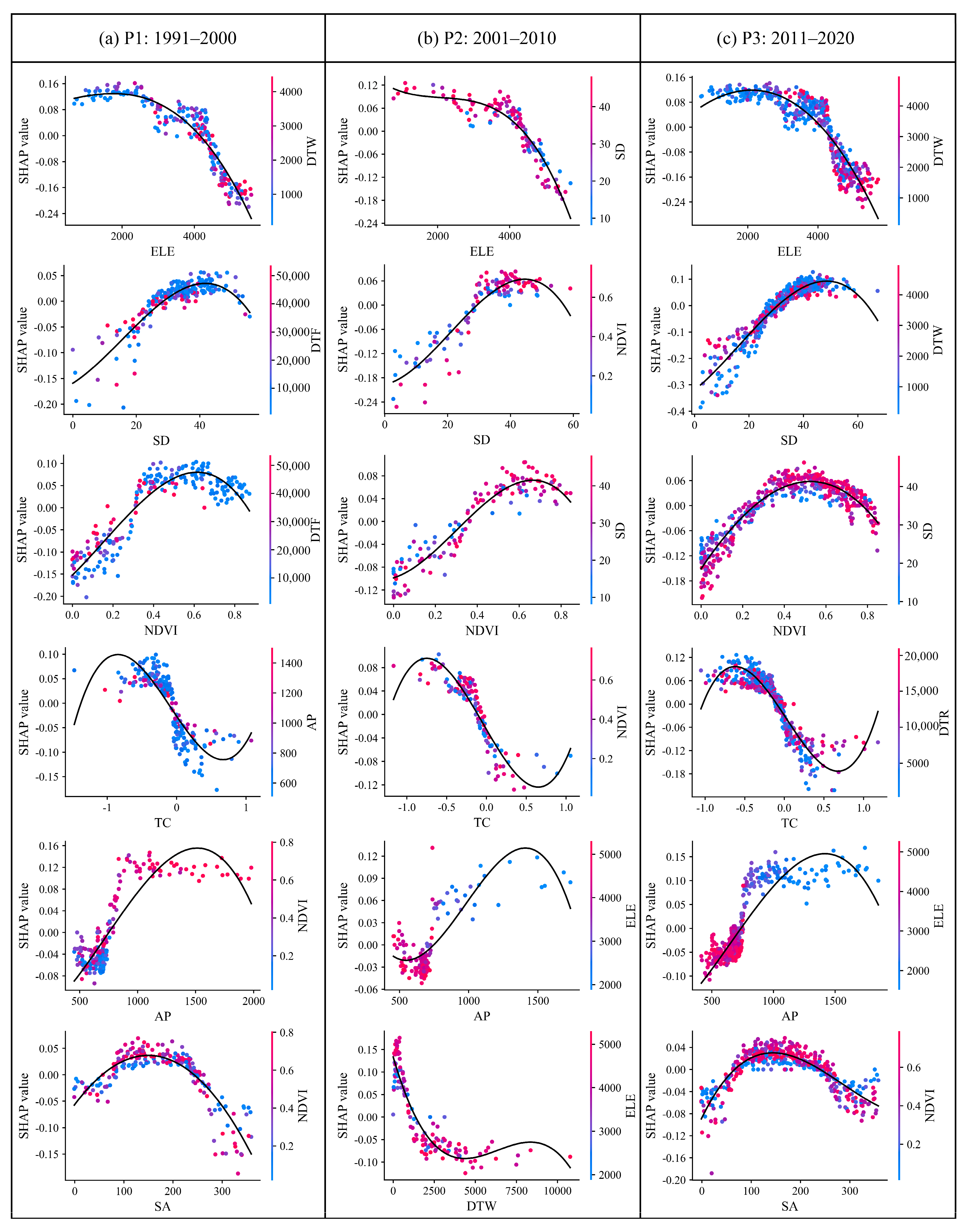
To examine the nonlinear associations between dominant factors and model-predicted landslide susceptibility, SHAP dependence plots were analyzed for the leading factors in each period. Figure 13 shows the nonlinear SHAP response patterns, and

Table 6. SHAP-derived nonlinear response types and key response ranges of dominant factors. T1 represents the main transition or zero-crossing point of the SHAP response, T2 represents the approximate peak, saturation, or attenuation-stabilization point, and SR represents the most sensitive response range. “—” indicates that no obvious threshold or response pattern was identified.

Factor	P1 (1991–2000)	P2 (2001–2010)	P3 (2011–2020)
ELE	Type I; T1 ≈ 4160 m; T2 ≈ 1760 m; SR: 1800–3500 m	Type I; T1 ≈ 4360 m; T2: —; SR: 2000–4000 m	Type I; T1 ≈ 4104 m; T2 ≈ 2114 m; SR: 2000–3500 m
SD	Type II; T1 ≈ 28.6°; T2 ≈ 42°; SR: 28–45°	Type II; T1 ≈ 29.3°; T2 ≈ 45°; SR: 30–45°	Type II; T1 ≈ 30.6°; T2 ≈ 48°; SR: 30–48°
NDVI	Type II; T1 ≈ 0.31; T2 ≈ 0.60; SR: 0.30–0.70	Type II; T1 ≈ 0.34; T2 ≈ 0.60; SR: 0.35–0.70	Type IV; T1 ≈ 0.26; T2 ≈ 0.53; SR: 0.25–0.65
TC	Type III; T1 ≈ −0.12; T2: —; SR: −0.70–0.20	Type III; T1 ≈ −0.11; T2: —; SR: −0.60–0.20	Type III; T1 ≈ −0.10; T2: —; SR: −0.60–0.20
AP	Type II; T1 ≈ 750 mm; T2 ≈ 1500 mm; SR: 750–1600 mm	Type II; T1 ≈ 748 mm; T2 ≈ 1400 mm; SR: 750–1500 mm	Type II; T1 ≈ 739 mm; T2 ≈ 1400 mm; SR: 750–1500 mm
DTW	—	Type I; T1 ≈ 1380 m; T2 ≈ 3500 m; SR: 0–2000 m	—
SA	Type IV; T1 ≈ 75°; T2 ≈ 150°; SR: 70–250°	—	Type IV; T1 ≈ 65.7°; T2 ≈ 143°; SR: 60–240°

summarizes the corresponding response types, approximate thresholds, and sensitive ranges derived from the smoothed SHAP trends. These thresholds should be interpreted as model-derived response ranges rather than deterministic physical breakpoints. The response patterns were classified into four types: overall decreasing or distance-decay responses (Type I), threshold-saturation responses (Type II), threshold-transition responses (Type III), and inverted U-shaped responses (Type IV). Together, these nonlinear response patterns indicate that landslide susceptibility in the Eastern Himalayan Syntaxis is controlled by the coupling between persistent geomorphic predisposition, characterized by deeply incised valleys and steep hillslopes, and stage-dependent modifiers such as rainfall, vegetation change, seismic disturbance, and drainage-corridor erosion.

As shown in Figure 13 and Table 6, several dominant factors exhibited relatively consistent nonlinear response patterns across the three periods. ELE showed an overall decreasing response after a low-to-middle-elevation positive contribution zone, with positive SHAP contributions mainly concentrated at approximately 1800–4000 m and declining markedly beyond about 4100–4360 m. SD displayed a stable threshold-saturation response, with the main transition threshold at approximately 28.6–30.6° and the most sensitive range around 28–48°. AP also showed a threshold-saturation pattern, with positive contributions generally emerging at approximately 739–750 mm and remaining high within about 750–1600 mm. TC exhibited a threshold-transition response, with the main transition near −0.12 to −0.10 and a sensitive range extending from negative to slightly positive curvature values, approximately −0.70 to 0.20.

In contrast, NDVI, DTW, and SA showed more evident period-specific responses. NDVI shifted from threshold-saturation responses in P1 and P2 to an inverted U-shaped response in P3. Its main transition occurred at approximately 0.31–0.34 in P1 and P2, with saturated contributions around 0.60, whereas the highest contribution in P3 occurred around 0.53, indicating that moderate vegetation-cover conditions became more important in the later period. The inverted U-shaped NDVI response in P3 may reflect the role of moderately vegetated slopes, which often correspond to disturbed or recovering surfaces such as post-landslide revegetation zones, valley-margin slopes, or areas affected by fluvial, seismic, or engineering disturbances. DTW appeared among the leading factors only in P2 and showed a clear distance-decay response, with high positive SHAP contributions concentrated within approximately 0–2000 m from drainage networks. SA displayed inverted U-shaped responses in P1 and P3, with peak contributions around 143–150°, suggesting locally important aspect-related contributions. Overall, the SHAP dependence plots complement the RI-based comparison by revealing both persistent nonlinear responses of topographic–geomorphic factors and period-specific responses of hydrological proximity and vegetation-related factors.

4. Discussion

4.1. Spatiotemporal Susceptibility Evolution

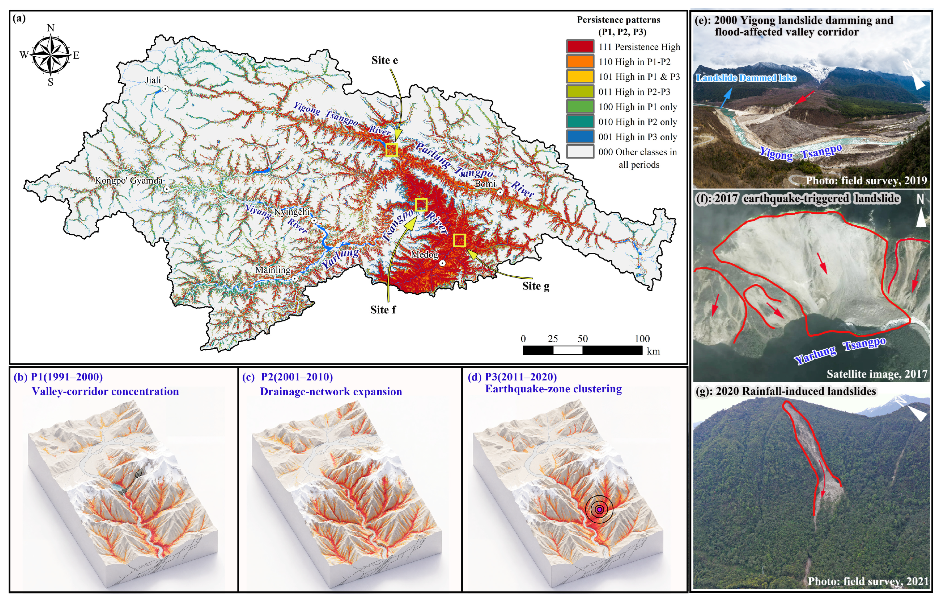
The multi-temporal susceptibility results reveal a persistent valley-controlled susceptibility pattern in the Eastern Himalayan Syntaxis. From 1991 to 2020, high and very high susceptibility zones were repeatedly concentrated along the Yarlung Tsangpo–Parlung Tsangpo–Yigong Tsangpo river system and major tributary junctions (Figure 8 and Figure 9), consistent with regional landslide studies [38,89,90]. The dominance of unchanged areas in the transition analysis indicates that the first-order susceptibility pattern remained stable at the decadal scale, whereas local class transitions along valley margins, tributary zones, and susceptibility hotspots suggest stage-dependent adjustment. The FR analysis further confirms that the mapped high-susceptibility zones correspond well to the spatial concentration of landslides.

Figure 14 synthesizes this pattern by linking susceptibility persistence, stage-wise reorganization, and representative disturbance scenarios. The persistence map highlights the long-term concentration of high and very high susceptibility along the main valley–tributary framework (Figure 14a), whereas the conceptual panels summarize the transition from main-valley aggregation in P1 (Figure 14b), to drainage-network expansion in P2 (Figure 14c), and to localized reconcentration near disturbed valley sections and tributary junctions in P3 (Figure 14d). This spatial organization reflects the high-relief valley setting of the Eastern Himalayan Syntaxis, where deeply incised rivers and steep valley-side slopes provide a long-term geomorphic template for landslide-prone terrain [32,91,92]. The representative cases shown in Figure 14e–g further illustrate typical fluvial, seismic, and rainfall-related disturbance pathways. The 2000 Yigong landslide-dammed river and flood-affected corridor, the 2017 earthquake-triggered landslide damming the Yarlung Tsangpo River, and the 2020 rainfall-induced landslide should therefore be interpreted as representative disturbances superimposed on a persistent valley–steep slope susceptibility framework, rather than as independent controls explaining the susceptibility pattern of individual periods.

4.2. Dominant Controls and SHAP Responses

The SHAP-based interpretation suggests that landslide susceptibility in the study area was shaped by the coupling between persistent geomorphic predisposition and period-dependent environmental or disturbance-related modifiers (Figure 10, Figure 11, Figure 12 and Figure 13; Table 5 and Table 6). This agrees with the view that landslide susceptibility reflects the combined influence of terrain, geological, hydrological, and environmental conditions rather than a single factor [12]. ELE, SD, and TC consistently represented the core topographic–geomorphic factors in the model-derived interpretation, reflecting terrain position, slope steepness, and local slope morphology. Their high RI values correspond to the repeated concentration of high and very high susceptibility zones along deeply incised valleys and steep hillslopes (Figure 14a), where strong relief, river incision, and threshold hillslope conditions commonly promote landslide development and erosion [9,91].

The nonlinear SHAP responses indicate that these geomorphic controls contributed to susceptibility predictions within specific sensitivity ranges rather than through simple linear effects. Low-to-middle-elevation valley belts, steep slopes, and curvature-controlled convergence or transition zones were the main geomorphic settings associated with high susceptibility predictions. Curvature-related responses may reflect the role of local slope geometry in runoff convergence, material redistribution, and slope-foot instability, consistent with previous findings that curvature-related terrain metrics are closely associated with landslide probability [93]. Thus, the persistent high-susceptibility pattern along the main valley system likely reflects the combined effects of elevation differentiation, steep hillslope morphology, active valley incision, and local terrain convergence.

On this geomorphic background, AP, NDVI, DTW, the PGA-like seismic disturbance proxy (SDI), and road proximity (DTR) further showed period-dependent relative associations with local susceptibility predictions. The threshold-like AP response suggests enhanced susceptibility under sufficient moisture conditions, but because AP represents period-averaged hydroclimatic conditions, it should not be interpreted as an event-scale rainfall threshold involving rainfall intensity, duration, or antecedent rainfall [94]. The period-dependent NDVI response indicates that vegetation-related relative importance was not uniformly stabilizing, as NDVI may also reflect hydroclimatic conditions, slope moisture, disturbance history, and post-disturbance recovery [95,96]. The prominence of DTW in P2 likely reflects drainage-corridor effects such as river incision and slope-foot erosion, whereas the enhanced relative importance of SDI in P3 may partly reflect the localized and late-period influence of the 2017 Nyingchi earthquake. This event triggered numerous coseismic landslides near the Yarlung Tsangpo Great Bend and the Parlung Tsangpo confluence, potentially promoting post-seismic weakening and delayed slope responses [97,98]. Overall, multi-temporal landslide susceptibility can be interpreted as reflecting the interaction between a persistent geomorphic template and stage-dependent hydroclimatic, fluvial, seismic, vegetation-related, and anthropogenic modifiers.

4.3. Implications and Limitations

The multi-temporal RF–SHAP framework provides a useful approach for distinguishing persistent high-susceptibility zones from areas with stage-specific susceptibility enhancement. Compared with conventional single-period susceptibility mapping, this framework introduces a temporal perspective into susceptibility assessment and helps identify where landslide-prone conditions remain stable or change over time. For high-relief valley regions such as the Eastern Himalayan Syntaxis, the results suggest that monitoring and mitigation should prioritize deeply incised river corridors, earthquake-affected slopes, tributary junctions, and road-affected valley sides.

Several uncertainties should also be acknowledged. Landslide inventory completeness may vary among periods because early-stage events are constrained by historical image quality, temporal coverage, and interpretation uncertainty. The selection of non-landslide samples may influence RF training and SHAP-based factor interpretation, and spatial autocorrelation between training and testing samples may lead to optimistic AUC estimates under the random-splitting strategy. The relatively lower AUC in P2 may also be related to its smaller landslide sample size and limited positive samples available for testing, while the use of identical RF hyperparameters across periods, although adopted for comparability, may introduce additional overfitting or underfitting uncertainty for the smaller P2 sample set. In addition, some conditioning factors represent period-averaged environmental states rather than event-scale triggers, limiting their ability to capture short-term rainfall, seismic, or engineering disturbances. Although RI normalization improves cross-period comparison, the independently trained RF models mean that temporal differences should be interpreted as relative changes in model-derived susceptibility rather than absolute changes in landslide probability. The resulting maps represent relative landslide susceptibility rather than landslide hazard or risk, because event probability, temporal frequency, runout intensity, exposure, and vulnerability were not explicitly modeled.

Future work should integrate event-scale rainfall records, InSAR-derived deformation, detailed road construction intensity, post-earthquake slope sensitivity indicators, and spatially independent validation strategies to strengthen physical constraints and improve adaptive susceptibility assessment in rapidly changing mountain environments.

5. Conclusions

This study established a 30-year landslide inventory for the Eastern Himalayan Syntaxis using long-term multi-source remote-sensing data. Period-specific RF models and Tree-SHAP interpretation were applied to assess landslide susceptibility evolution and dominant factor responses across P1 (1991–2000), P2 (2001–2010), and P3 (2011–2020). The main conclusions are as follows:

(1)

The three RF models showed reliable predictive performance, with AUC values of 0.887, 0.848, and 0.900 for P1, P2, and P3, respectively, supporting period-specific susceptibility mapping and interpretation.

(2)

Landslide susceptibility exhibited broad temporal stability with localized reorganization. Unchanged areas dominated the P1–P2, P2–P3, and P1–P3 transitions, accounting for 55.62%, 51.62%, and 58.51% of the study area, respectively. High and very high susceptibility zones were persistently concentrated along the Yarlung Tsangpo–Parlung Tsangpo–Yigong Tsangpo river system and major tributary junctions, indicating strong geomorphic control by deeply incised valleys and steep hillslopes.

(3)

SHAP-based interpretation showed that ELE, SD, TC, NDVI, and AP formed the shared core factor group, whereas DTW, the seismic disturbance proxy, and road proximity showed stronger stage-dependent variations. The cumulative RI values of the top six factors reached 81.1%, 86.7%, and 83.2% in P1, P2, and P3, respectively.

(4)

The dominant factors influenced model-predicted susceptibility mainly through nonlinear responses, including threshold-saturation, overall decreasing or distance-decay, threshold-transition, and inverted U-shaped patterns. Overall, susceptibility evolution reflects the coupling between persistent geomorphic predisposition and stage-dependent hydroclimatic, fluvial, seismic, vegetation-related, and anthropogenic modifiers. The proposed multi-temporal RF–SHAP framework provides a useful basis for identifying persistent and stage-specific high-susceptibility zones in high-relief valley regions.

References

1. Hungr, O.; Leroueil, S.; Picarelli, L. The Varnes Classification of Landslide Types, an Update. Landslides 2014, 11, 167–194. [Google Scholar] [CrossRef]
2. Gariano, S.L.; Guzzetti, F. Landslides in a Changing Climate. Earth-Sci. Rev. 2016, 162, 227–252. [Google Scholar] [CrossRef]
3. Korup, O.; Clague, J.J.; Hermanns, R.L.; Hewitt, K.; Strom, A.L.; Weidinger, J.T. Giant Landslides, Topography, and Erosion. Earth Planet. Sci. Lett. 2007, 261, 578–589. [Google Scholar] [CrossRef]
4. Petley, D. Global Patterns of Loss of Life from Landslides. Geology 2012, 40, 927–930. [Google Scholar] [CrossRef]
5. Luo, H.Y.; Zhang, L.M.; Zhang, L.L.; He, J.; Yin, K.S. Vulnerability of Buildings to Landslides: The State of the Art and Future Needs. Earth-Sci. Rev. 2023, 238, 104329. [Google Scholar] [CrossRef]
6. Fan, X.; Yang, F.; Siva Subramanian, S.; Xu, Q.; Feng, Z.; Mavrouli, O.; Peng, M.; Ouyang, C.; Jansen, J.D.; Huang, R. Prediction of a Multi-Hazard Chain by an Integrated Numerical Simulation Approach: The Baige Landslide, Jinsha River, China. Landslides 2020, 17, 147–164. [Google Scholar] [CrossRef]
7. Mani, P.; Allen, S.; Evans, S.G.; Kargel, J.S.; Mergili, M.; Petrakov, D.; Stoffel, M. Geomorphic Process Chains in High-Mountain Regions—A Review and Classification Approach for Natural Hazards Assessment. Rev. Geophys. 2023, 61, e2022RG000791. [Google Scholar] [CrossRef]
8. Fell, R.; Corominas, J.; Bonnard, C.; Cascini, L.; Leroi, E.; Savage, W.Z. Guidelines for Landslide Susceptibility, Hazard and Risk Zoning for Land Use Planning. Eng. Geol. 2008, 102, 85–98. [Google Scholar] [CrossRef]
9. Zhao, S.; Dai, F.; Deng, J.; Wen, H.; Li, H.; Chen, F. Insights into Landslide Development and Susceptibility in Extremely Complex Alpine Geoenvironments along the Western Sichuan–Tibet Engineering Corridor, China. CATENA 2023, 227, 107105. [Google Scholar] [CrossRef]
10. Guzzetti, F.; Mondini, A.C.; Cardinali, M.; Fiorucci, F.; Santangelo, M.; Chang, K.-T. Landslide Inventory Maps: New Tools for an Old Problem. Earth-Sci. Rev. 2012, 112, 42–66. [Google Scholar] [CrossRef]
11. Huang, F.; Mao, D.; Jiang, S.-H.; Zhou, C.; Fan, X.; Zeng, Z.; Catani, F.; Yu, C.; Chang, Z.; Huang, J.; et al. Uncertainties in Landslide Susceptibility Prediction Modeling: A Review on the Incompleteness of Landslide Inventory and Its Influence Rules. Geosci. Front. 2024, 15, 101886. [Google Scholar] [CrossRef]
12. Reichenbach, P.; Rossi, M.; Malamud, B.D.; Mihir, M.; Guzzetti, F. A Review of Statistically-Based Landslide Susceptibility Models. Earth-Sci. Rev. 2018, 180, 60–91. [Google Scholar] [CrossRef]
13. Achu, A.L.; Aju, C.D.; Di Napoli, M.; Prakash, P.; Gopinath, G.; Shaji, E.; Chandra, V. Machine-Learning Based Landslide Susceptibility Modelling with Emphasis on Uncertainty Analysis. Geosci. Front. 2023, 14, 101657. [Google Scholar] [CrossRef]
14. Li, L.; Lan, H.; Guo, C.; Zhang, Y.; Li, Q.; Wu, Y. A Modified Frequency Ratio Method for Landslide Susceptibility Assessment. Landslides 2017, 14, 727–741. [Google Scholar] [CrossRef]
15. Zhang, Y.; Lan, H.; Li, L.; Wu, Y.; Chen, J.; Tian, N. Optimizing the Frequency Ratio Method for Landslide Susceptibility Assessment: A Case Study of the Caiyuan Basin in the Southeast Mountainous Area of China. J. Mt. Sci. 2020, 17, 340–357. [Google Scholar] [CrossRef]
16. Wei, R.; Ye, C.; Sui, T.; Ge, Y.; Li, Y.; Li, J. Combining Spatial Response Features and Machine Learning Classifiers for Landslide Susceptibility Mapping. Int. J. Appl. Earth Obs. Geoinf. 2022, 107, 102681. [Google Scholar] [CrossRef]
17. Huang, W.; Ding, M.; Li, Z.; Yu, J.; Ge, D.; Liu, Q.; Yang, J. Landslide Susceptibility Mapping and Dynamic Response along the Sichuan-Tibet Transportation Corridor Using Deep Learning Algorithms. CATENA 2023, 222, 106866. [Google Scholar] [CrossRef]
18. Wei, Y.; Qiu, H.; Liu, Z.; Huangfu, W.; Zhu, Y.; Liu, Y.; Yang, D.; Kamp, U. Refined and Dynamic Susceptibility Assessment of Landslides Using InSAR and Machine Learning Models. Geosci. Front. 2024, 15, 101890. [Google Scholar] [CrossRef]
19. Breiman, L. Random Forests. Mach. Learn. 2001, 45, 5–32. [Google Scholar] [CrossRef]
20. Sun, D.; Xu, J.; Wen, H.; Wang, D. Assessment of Landslide Susceptibility Mapping Based on Bayesian Hyperparameter Optimization: A Comparison between Logistic Regression and Random Forest. Eng. Geol. 2021, 281, 105972. [Google Scholar] [CrossRef]
21. Liu, S.; Jiang, X.; He, X.; Qiu, H.; Yang, Y.; Zhao, R.; Hu, H. A Novel Landslide Susceptibility Mapping Method Based on a Backpropagation Neural Network Algorithm with Optimized Non-Landslide Samples and Hyperparameters. Eng. Appl. Artif. Intell. 2025, 155, 111052. [Google Scholar] [CrossRef]
22. Merghadi, A.; Yunus, A.P.; Dou, J.; Whiteley, J.; ThaiPham, B.; Bui, D.T.; Avtar, R.; Abderrahmane, B. Machine Learning Methods for Landslide Susceptibility Studies: A Comparative Overview of Algorithm Performance. Earth-Sci. Rev. 2020, 207, 103225. [Google Scholar] [CrossRef]
23. Ado, M.; Amitab, K.; Maji, A.K.; Jasińska, E.; Gono, R.; Leonowicz, Z.; Jasiński, M. Landslide Susceptibility Mapping Using Machine Learning: A Literature Survey. Remote Sens. 2022, 14, 3029. [Google Scholar] [CrossRef]
24. Zhou, X.; Wen, H.; Zhang, Y.; Xu, J.; Zhang, W. Landslide Susceptibility Mapping Using Hybrid Random Forest with GeoDetector and RFE for Factor Optimization. Geosci. Front. 2021, 12, 101211. [Google Scholar] [CrossRef]
25. He, Y.; Ding, M.; Duan, Y.; Zheng, H.; Wu, J.; Feng, L. Exploring the Dynamic Impact of Urbanization on Landslide Susceptibility in Sichuan Province Using an Explainable XGBoost Model. Eng. Geol. 2025, 357, 108372. [Google Scholar] [CrossRef]
26. Lundberg, S.; Lee, S.-I. A Unified Approach to Interpreting Model Predictions. In Proceedings of the 31st Conference on Neural Information Processing Systems, Long Beach, CA, USA, 4–9 December 2017. [Google Scholar]
27. Dahal, A.; Lombardo, L. Explainable Artificial Intelligence in Geoscience: A Glimpse into the Future of Landslide Susceptibility Modeling. Comput. Geosci. 2023, 176, 105364. [Google Scholar] [CrossRef]
28. Lv, J.; Zhang, R.; Shama, A.; Hong, R.; He, X.; Wu, R.; Bao, X.; Liu, G. Exploring the Spatial Patterns of Landslide Susceptibility Assessment Using Interpretable Shapley Method: Mechanisms of Landslide Formation in the Sichuan-Tibet Region. J. Environ. Manag. 2024, 366, 121921. [Google Scholar] [CrossRef]
29. Xu, F.; Xu, Q.; Pu, C.; Wang, X.; Xu, P. Can Different Machine Learning Methods Have Consistent Interpretations of DEM-Based Factors in Shallow Landslide Susceptibility Assessments? J. Rock Mech. Geotech. Eng. 2025, 17, 7864–7881. [Google Scholar] [CrossRef]
30. Ma, P.; Chen, L.; Yu, C.; Zhu, Q.; Ding, Y.; Wu, Z.; Li, H.; Tian, C.; Fan, X. Dynamic Landslide Susceptibility Mapping over Last Three Decades to Uncover Variations in Landslide Causation in Subtropical Urban Mountainous Areas. Remote Sens. Environ. 2025, 326, 114800. [Google Scholar] [CrossRef]
31. Ding, L.; Zhong, D.; Yin, A.; Kapp, P.; Harrison, T.M. Cenozoic Structural and Metamorphic Evolution of the Eastern Himalayan Syntaxis (Namche Barwa). Earth Planet. Sci. Lett. 2001, 192, 423–438. [Google Scholar] [CrossRef]
32. Finnegan, N.J.; Hallet, B.; Montgomery, D.R.; Zeitler, P.K.; Stone, J.O.; Anders, A.M.; Yuping, L. Coupling of Rock Uplift and River Incision in the Namche Barwa-Gyala Peri Massif, Tibet. Geol. Soc. Am. Bull. 2008, 120, 142–155. [Google Scholar] [CrossRef]
33. Zhao, B.; Su, L. Complex Spatial and Size Distributions of Landslides in the Yarlung Tsangpo River (YTR) Basin. J. Rock Mech. Geotech. Eng. 2025, 17, 897–914. [Google Scholar] [CrossRef]
34. Delaney, K.B.; Evans, S.G. The 2000 Yigong Landslide (Tibetan Plateau), Rockslide-Dammed Lake and Outburst Flood: Review, Remote Sensing Analysis, and Process Modelling. Geomorphology 2015, 246, 377–393. [Google Scholar] [CrossRef]
35. Zhang, Q.; Hu, K.; Wei, L.; Liu, W. Rapid Changes in Fluvial Morphology in Response to the High-Energy Yigong Outburst Flood in 2000: Integrating Channel Dynamics and Flood Hydraulics. J. Hydrol. 2022, 612, 128199. [Google Scholar] [CrossRef]
36. Zhao, B.; Li, W.; Wang, Y.; Lu, J.; Li, X. Landslides Triggered by the Ms 6.9 Nyingchi Earthquake, China (18 November 2017): Analysis of the Spatial Distribution and Occurrence Factors. Landslides 2019, 16, 765–776. [Google Scholar] [CrossRef]
37. Wang, X.; Clague, J.J.; Crosta, G.B.; Sun, J.; Stead, D.; Qi, S.; Zhang, L. Relationship between the Spatial Distribution of Landslides and Rock Mass Strength, and Implications for the Driving Mechanism of Landslides in Tectonically Active Mountain Ranges. Eng. Geol. 2021, 292, 106281. [Google Scholar] [CrossRef]
38. Du, G.; Zhang, Y.; Gu, L.; Yang, Z.; Ren, S.; Yuan, S. A Systematic Approach to Landslide Susceptibility Assessment in Regions of Rapid Geomorphic Evolution: A Case Study of the Yarlung Zangbo Grand Bend. Bull. Eng. Geol. Environ. 2025, 84, 581. [Google Scholar] [CrossRef]
39. Guo, C.; Montgomery, D.R.; Zhang, Y.; Zhong, N.; Fan, C.; Wu, R.; Yang, Z.; Ding, Y.; Jin, J.; Yan, Y. Evidence for Repeated Failure of the Giant Yigong Landslide on the Edge of the Tibetan Plateau. Sci. Rep. 2020, 10, 14371. [Google Scholar] [CrossRef]
40. Uwizeyimana, D.; Liu, W.; Huang, Y.; Habumugisha, J.M.; Zhou, Y.; Yang, Z. Spatial Distribution Characteristics of Climate-Induced Landslides in the Eastern Himalayas. J. Mt. Sci. 2024, 21, 3396–3412. [Google Scholar] [CrossRef]
41. Wang, P.; Scherler, D.; Liu-Zeng, J.; Mey, J.; Avouac, J.-P.; Zhang, Y.; Shi, D. Tectonic Control of Yarlung Tsangpo Gorge Revealed by a Buried Canyon in Southern Tibet. Science 2014, 346, 978–981. [Google Scholar] [CrossRef]
42. Ma, Y.; Lu, M.; Bracken, C.; Chen, H. Spatially Coherent Clusters of Summer Precipitation Extremes in the Tibetan Plateau: Where Is the Moisture From? Atmos. Res. 2020, 237, 104841. [Google Scholar] [CrossRef]
43. Wang, C.; Mooney, W.D.; Zhu, L.; Wang, X.; Lou, H.; You, H.; Cao, Z.; Chang, L.; Yao, Z. Deep Structure of the Eastern Himalayan Collision Zone: Evidence for Underthrusting and Delamination in the Postcollisional Stage. Tecton. 2019, 38, 3614–3628. [Google Scholar] [CrossRef]
44. Liu, S.; Lan, H.; Strom, A.; Li, L.; Bao, H. Spatial Segmentation of Jiali Fault’s Holocene Activity in the Southeastern Tibetan Plateau. npj Nat. Hazards 2024, 1, 42. [Google Scholar] [CrossRef]
45. Zhang, Z.; Dong, X.; Santosh, M.; Liu, F.; Wang, W.; Yiu, F.; He, Z.; Shen, K. Petrology and Geochronology of the Namche Barwa Complex in the Eastern Himalayan Syntaxis, Tibet: Constraints on the Origin and Evolution of the North-Eastern Margin of the Indian Craton. Gondwana Res. 2012, 21, 123–137. [Google Scholar] [CrossRef]
46. Liu, S.; Lan, H.; Martin, C.D. Effect of Disturbance on the Progressive Failure Process of Eastern Himalayan Gneiss. Eng. Geol. 2023, 312, 106936. [Google Scholar] [CrossRef]
47. Wei, R.; Zeng, Q.; Davies, T.; Yuan, G.; Wang, K.; Xue, X.; Yin, Q. Geohazard Cascade and Mechanism of Large Debris Flows in Tianmo Gully, SE Tibetan Plateau and Implications to Hazard Monitoring. Eng. Geol. 2018, 233, 172–182. [Google Scholar] [CrossRef]
48. Gao, H.; Gao, Y.; Li, B.; Yin, Y.; Yang, C.; Wan, J.; Zhang, T. The Dynamic Simulation and Potential Hazards Analysis of the Yigong Landslide in Tibet, China. Remote Sens. 2023, 15, 1322. [Google Scholar] [CrossRef]
49. Zhang, Y.; Yin, Y.; Li, B.; Tie, Y.; Li, C.; Gao, Y.; Wang, M.; Wang, L. Geostructural Characteristics and Failure Mechanism of the Benduo Mountain Slope in the Yigong Zangbo River, Qinghai–Tibet Plateau, China. Landslides 2025, 22, 2005–2020. [Google Scholar] [CrossRef]
50. Zhang, Z.; Sun, J. Regional Landslide Susceptibility Assessment and Model Adaptability Research. Remote Sens. 2024, 16, 2305. [Google Scholar] [CrossRef]
51. Wu, X.; Xu, X.; Yu, G.; Ren, J.; Yang, X.; Chen, G.; Xu, C.; Du, K.; Huang, X.; Yang, H.; et al. The China Active Faults Database (CAFD) and Its Web System. Earth Syst. Sci. Data 2024, 16, 3391–3417. [Google Scholar] [CrossRef]
52. Rabby, Y.W.; Li, Y. An Integrated Approach to Map Landslides in Chittagong Hilly Areas, Bangladesh, Using Google Earth and Field Mapping. Landslides 2019, 16, 633–645. [Google Scholar] [CrossRef]
53. Pu, C.; Xu, Q.; Wang, X.; Li, Z.; Chen, W.; Zhao, K.; Xiu, D.; Liu, J. Refined Mapping and Kinematic Trend Assessment of Potential Landslides Associated with Large-Scale Land Creation Projects with Multitemporal InSAR. Int. J. Appl. Earth Obs. Geoinf. 2023, 118, 103266. [Google Scholar] [CrossRef]
54. Novellino, A.; Pennington, C.; Leeming, K.; Taylor, S.; Alvarez, I.G.; McAllister, E.; Arnhardt, C.; Winson, A. Mapping Landslides from Space: A Review. Landslides 2024, 21, 1041–1052. [Google Scholar] [CrossRef]
55. Kovalskyy, V.; Roy, D.P. The Global Availability of Landsat 5 TM and Landsat 7 ETM+ Land Surface Observations and Implications for Global 30m Landsat Data Product Generation. Remote Sens. Environ. 2013, 130, 280–293. [Google Scholar] [CrossRef]
56. Gao, X.; Gray, J.M.; Reich, B.J. Long-Term, Medium Spatial Resolution Annual Land Surface Phenology with a Bayesian Hierarchical Model. Remote Sens. Environ. 2021, 261, 112484. [Google Scholar] [CrossRef]
57. Hongying, L.; Fenggui, L.; Qiong, C.; Xingsheng, X. Monthly NDVI Spatial and Temporal Fusion Dataset at 250 m Resolution on the Tibetan Plateau 1981–2020; Science Data Bank: Xining, China, 2024. [Google Scholar]
58. Gao, X.; Sun, D. Transport Accessibility and Social Demand: A Case Study of the Tibetan Plateau. PLoS ONE 2021, 16, e0257028. [Google Scholar] [CrossRef]
59. Görüm, T. Tectonic, Topographic and Rock-Type Influences on Large Landslides at the Northern Margin of the Anatolian Plateau. Landslides 2019, 16, 333–346. [Google Scholar] [CrossRef]
60. Reyes-Carmona, C.; Galve, J.P.; Pérez-Peña, J.V.; Moreno-Sánchez, M.; Alfonso-Jorde, D.; Ballesteros, D.; Torre, D.; Azañón, J.M.; Mateos, R.M. Improving Landslide Inventories by Combining Satellite Interferometry and Landscape Analysis: The Case of Sierra Nevada (Southern Spain). Landslides 2023, 20, 1815–1835. [Google Scholar] [CrossRef]
61. Ozturk, U.; Pittore, M.; Behling, R.; Roessner, S.; Andreani, L.; Korup, O. How Robust Are Landslide Susceptibility Estimates? Landslides 2021, 18, 681–695. [Google Scholar] [CrossRef]
62. Martha, T.R.; Kerle, N.; Jetten, V.; Van Westen, C.J.; Kumar, K.V. Characterising Spectral, Spatial and Morphometric Properties of Landslides for Semi-Automatic Detection Using Object-Oriented Methods. Geomorphology 2010, 116, 24–36. [Google Scholar] [CrossRef]
63. Cruden, D.M.; Varnes, D.J. Landslide Types and Processes. Spec. Rep. Natl. Res. Counc. Transp. Res. Board 1996, 247, 36–75. [Google Scholar]
64. Guo, C.; Montgomery, D.R.; Zhang, Y.; Wang, K.; Yang, Z. Quantitative Assessment of Landslide Susceptibility along the Xianshuihe Fault Zone, Tibetan Plateau, China. Geomorphology 2015, 248, 93–110. [Google Scholar] [CrossRef]
65. Feizizadeh, B.; Blaschke, T. GIS-Multicriteria Decision Analysis for Landslide Susceptibility Mapping: Comparing Three Methods for the Urmia Lake Basin, Iran. Nat. Hazards 2013, 65, 2105–2128. [Google Scholar] [CrossRef]
66. Feizizadeh, B.; Blaschke, T. An Uncertainty and Sensitivity Analysis Approach for GIS-Based Multicriteria Landslide Susceptibility Mapping. Int. J. Geogr. Inf. Sci. 2014, 28, 610–638. [Google Scholar] [CrossRef]
67. Guo, Z.; Shi, Y.; Huang, F.; Fan, X.; Huang, J. Landslide Susceptibility Zonation Method Based on C5.0 Decision Tree and K-Means Cluster Algorithms to Improve the Efficiency of Risk Management. Geosci. Front. 2021, 12, 101249. [Google Scholar] [CrossRef]
68. Qi, S. Engineering Geological Petrofabric Database of Qinghai Tibet Plateau, 2021; National Tibetan Plateau Data Center: Beijing, China, 2021; Available online: https://cstr.cn/18406.11.SolidEar.tpdc.272211 (accessed on 24 July 2025).
69. Peng, S.; Ding, Y.; Liu, W.; Li, Z. 1 Km Monthly Temperature and Precipitation Dataset for China from 1901 to 2017. Earth Syst. Sci. Data 2019, 11, 1931–1946. [Google Scholar] [CrossRef]
70. Peng, S. 1-Km Monthly Precipitation Dataset for China (1901–2024); National Earth System Science Data Center: Beijing, China, 2025. [Google Scholar]
71. Wald, D.; Quitoriano, V.; Heaton, T.; Kanamori, H.; Scrivner, C.; Worden, C.B. TriNet “ShakeMaps”: Rapid Generation of Peak Ground Motion and Intensity Maps for Earthquakes in Southern California. Earthq. Spectra 1999, 15, 537–555. [Google Scholar] [CrossRef]
72. Wald, D.; Worden, B.; Quitoriano, V.; Pankow, K. ShakeMap Manual: Technical Manual, User’s Guide, and Software Guide; Techniques and Methods; Version 1.0.; U.S. Geological Survey: Reston, VA, USA, 2005.
73. Worden, C.B.; Wald, D.J.; Allen, T.I.; Lin, K.; Garcia, D.; Cua, G. A Revised Ground-Motion and Intensity Interpolation Scheme for ShakeMap. Bull. Seismol. Soc. Am. 2010, 100, 3083–3096. [Google Scholar] [CrossRef]
74. Tien Bui, D.; Tuan, T.A.; Klempe, H.; Pradhan, B.; Revhaug, I. Spatial Prediction Models for Shallow Landslide Hazards: A Comparative Assessment of the Efficacy of Support Vector Machines, Artificial Neural Networks, Kernel Logistic Regression, and Logistic Model Tree. Landslides 2016, 13, 361–378. [Google Scholar] [CrossRef]
75. Lin, G.-F.; Chang, M.-J.; Huang, Y.-C.; Ho, J.-Y. Assessment of Susceptibility to Rainfall-Induced Landslides Using Improved Self-Organizing Linear Output Map, Support Vector Machine, and Logistic Regression. Eng. Geol. 2017, 224, 62–74. [Google Scholar] [CrossRef]
76. Sun, D.; Shi, S.; Wen, H.; Xu, J.; Zhou, X.; Wu, J. A Hybrid Optimization Method of Factor Screening Predicated on GeoDetector and Random Forest for Landslide Susceptibility Mapping. Geomorphology 2021, 379, 107623. [Google Scholar] [CrossRef]
77. Gu, T.; Li, J.; Wang, M.; Duan, P.; Zhang, Y.; Cheng, L. Study on Landslide Susceptibility Mapping with Different Factor Screening Methods and Random Forest Models. PLoS ONE 2023, 18, e0292897. [Google Scholar] [CrossRef] [PubMed]
78. Tanyu, B.F.; Abbaspour, A.; Alimohammadlou, Y.; Tecuci, G. Landslide Susceptibility Analyses Using Random Forest, C4.5, and C5.0 with Balanced and Unbalanced Datasets. CATENA 2021, 203, 105355. [Google Scholar] [CrossRef]
79. Chen, W.; Li, X.; Wang, Y.; Chen, G.; Liu, S. Forested Landslide Detection Using LiDAR Data and the Random Forest Algorithm: A Case Study of the Three Gorges, China. Remote Sens. Environ. 2014, 152, 291–301. [Google Scholar] [CrossRef]
80. Krkač, M.; Špoljarić, D.; Bernat, S.; Arbanas, S.M. Method for Prediction of Landslide Movements Based on Random Forests. Landslides 2017, 14, 947–960. [Google Scholar] [CrossRef]
81. Yang, L.; Cui, Y.; Xu, C.; Ma, S. Application of Coupling Physics–Based Model TRIGRS with Random Forest in Rainfall-Induced Landslide-Susceptibility Assessment. Landslides 2024, 21, 2179–2193. [Google Scholar] [CrossRef]
82. Zheng, D.; Li, Y.; Yan, C.; Wu, H.; Yamashiki, Y.A.; Gao, B.; Nian, T. Landslide Susceptibility Assessment Using AutoML-SHAP Method in the Southern Foothills of Changbai Mountain, China. Landslides 2025, 22, 1855–1875. [Google Scholar] [CrossRef]
83. Li, B.; Wang, G.; Chen, L.; Sun, F.; Wang, R.; Liao, M.; Xu, H.; Li, S.; Kang, Y. Analysis of Landslide Deformation Mechanisms and Coupling Effects under Rainfall and Reservoir Water Level Effects. Eng. Geol. 2024, 343, 107803. [Google Scholar] [CrossRef]
84. Li, L.; Lan, H. Bivariate Landslide Susceptibility Analysis: Clarification, Optimization, Open Software, and Preliminary Comparison. Remote Sens. 2023, 15, 1418. [Google Scholar] [CrossRef]
85. Li, L.; Lan, H. Analytical ‘Decisiveness’ as a Robust Measure of the Absolute Importance of Landslide Predisposing Factors. Int. J. Digit. Earth 2024, 17, 2356161. [Google Scholar] [CrossRef]
86. Deng, Z.; Lan, H.; Li, L.; Liu, Y.; Tian, N. A Catchment-Scale Landslide Hydro-Mechanical Coupling Model Considering Spatial Heterogeneity. J. Hydrol. 2026, 667, 134855. [Google Scholar] [CrossRef]
87. Wang, Y.; Feng, L.; Li, S.; Ren, F.; Du, Q. A Hybrid Model Considering Spatial Heterogeneity for Landslide Susceptibility Mapping in Zhejiang Province, China. CATENA 2020, 188, 104425. [Google Scholar] [CrossRef]
88. Qin, X.; Huang, Y.; Wang, C.; Jiang, K.; Xie, L.; Liu, R.; Shi, X.; Chen, X.; Zhang, B. A Temporary Soil Dump Settlement and Landslide Risk Analysis Using the Improved Small Baseline Subset-InSAR and Continuous Medium Model. Int. J. Appl. Earth Obs. Geoinf. 2024, 128, 103760. [Google Scholar] [CrossRef]
89. Du, G.; Zhang, Y.; Yang, Z.; Guo, C.; Yao, X.; Sun, D. Landslide Susceptibility Mapping in the Region of Eastern Himalayan Syntaxis, Tibetan Plateau, China: A Comparison between Analytical Hierarchy Process Information Value and Logistic Regression-Information Value Methods. Bull. Eng. Geol. Environ. 2019, 78, 4201–4215. [Google Scholar] [CrossRef]
90. Jia, W.-J.; Wang, M.-F.; Zhou, C.-H.; Yang, Q.-H. Analysis of the Spatial Association of Geographical Detector-Based Landslides and Environmental Factors in the Southeastern Tibetan Plateau, China. PLoS ONE 2021, 16, e0251776. [Google Scholar] [CrossRef]
91. Larsen, I.J.; Montgomery, D.R. Landslide Erosion Coupled to Tectonics and River Incision. Nat. Geosci. 2012, 5, 468–473. [Google Scholar] [CrossRef]
92. Lang, K.A.; Huntington, K.W.; Burmester, R.; Housen, B. Rapid Exhumation of the Eastern Himalayan Syntaxis since the Late Miocene. Geol. Soc. Am. Bull. 2016, 128, 1403–1422. [Google Scholar] [CrossRef]
93. Ohlmacher, G.C. Plan Curvature and Landslide Probability in Regions Dominated by Earth Flows and Earth Slides. Eng. Geol. 2007, 91, 117–134. [Google Scholar] [CrossRef]
94. Guzzetti, F.; Peruccacci, S.; Rossi, M.; Stark, C.P. The Rainfall Intensity–Duration Control of Shallow Landslides and Debris Flows: An Update. Landslides 2008, 5, 3–17. [Google Scholar] [CrossRef]
95. Chen, L.; Guo, Z.; Yin, K.; Shrestha, D.P.; Jin, S. The Influence of Land Use and Land Cover Change on Landslide Susceptibility: A Case Study in Zhushan Town, Xuan’en County (Hubei, China). Nat. Hazards Earth Syst. Sci. 2019, 19, 2207–2228. [Google Scholar] [CrossRef]
96. Pacheco Quevedo, R.; Velastegui-Montoya, A.; Montalván-Burbano, N.; Morante-Carballo, F.; Korup, O.; Daleles Rennó, C. Land Use and Land Cover as a Conditioning Factor in Landslide Susceptibility: A Literature Review. Landslides 2023, 20, 967–982. [Google Scholar] [CrossRef]
97. Fan, X.; Yunus, A.P.; Scaringi, G.; Catani, F.; Siva Subramanian, S.; Xu, Q.; Huang, R. Rapidly Evolving Controls of Landslides After a Strong Earthquake and Implications for Hazard Assessments. Geophys. Res. Lett. 2021, 48, e2020GL090509. [Google Scholar] [CrossRef]
98. Tanyaş, H.; Kirschbaum, D.; Görüm, T.; Van Westen, C.J.; Tang, C.; Lombardo, L. A Closer Look at Factors Governing Landslide Recovery Time in Post-Seismic Periods. Geomorphology 2021, 391, 107912. [Google Scholar] [CrossRef]
Figure 2. Landslide inventory and temporal partitioning. (a,b) Representative pre- and post-event Google Earth images for determining landslide occurrence timing. the red dashed line in (b) indicates the interpreted landslide boundary; (c) Distribution of all mapped landslides from 1991 to 2020; (df) Landslide distributions in P1 (1991–2000), P2 (2001–2010), P3 (2011–2020), respectively.
Remotesensing 18 01842 g002
Figure 3. Static conditioning factors. (a) Elevation (ELE); (b) Slope gradient (SD); (c) Slope aspect (SA); (d) Terrain relief (TR); (e) Terrain curvature (TC); (f) Lithology (LT); (g) Distance to fault (DTF); (h) Distance to water (DTW).
Remotesensing 18 01842 g003
Figure 4. Dynamic conditioning factors. (ac) Decadal mean annual precipitation (AP); (df) Decadal mean normalized difference vegetation index (NDVI); (gi) Distance to roads (DTR); (jl) Seismic disturbance proxy index (SDI).
Remotesensing 18 01842 g004
Figure 5. Flowchart of the framework in this study.
Remotesensing 18 01842 g005
Figure 6. Correlation Heatmap of Influencing Factors.
Remotesensing 18 01842 g006
Figure 7. ROC curves of the period-specific landslide susceptibility models. (a) P1: 1991–2000; (b) P2: 2001–2010; (c) P3: 2011–2020. The diagonal dashed line in the ROC plots represents the random-classification baseline.
Remotesensing 18 01842 g007
Figure 8. Landslide susceptibility maps and class statistics for the three periods. (ac) Susceptibility maps for P1, P2, and P3; (d) area and landslide ratios of different susceptibility classes. The dashed line separates the area ratios of the susceptibility classes on the left from the landslide ratios on the right.
Remotesensing 18 01842 g008
Figure 9. Transitions in landslide susceptibility classes across periods. (a) P1–P2 transition; (b) P2–P3 transition; (c) P1–P3 transition;and (d) Proportions of different transition types. The colors in (ac) represent different susceptibility classes.
Remotesensing 18 01842 g009
Figure 10. SHAP-based global importance of conditioning factors. (ac) SHAP beeswarm plots for P1, P2, and P3, respectively. Each point represents one sample, and point colours indicate factor values, with red representing higher values and blue representing lower values; (df) Mean(|SHAP|) rankings of conditioning factors for P1, P2, and P3, respectively.
Remotesensing 18 01842 g010
Figure 11. Temporal variation in the relative importance of conditioning factors. (a) Relative importance index (RI) of individual conditioning factors across the three periods; (b) per-factor average RI of static and dynamic factor groups.
Remotesensing 18 01842 g011
Figure 12. Temporal ranking of SHAP-based factor importance. (a) Period-specific ranking of conditioning factors derived from the relative importance index (RI) based on mean absolute SHAP values; (b) average rank of each conditioning factor across the three periods.
Remotesensing 18 01842 g012
Figure 13. SHAP dependence plots of dominant factors across the three periods. (a) P1: 1991–2000; (b) P2: 2001–2010; and (c) P3: 2011–2020. Each subplot shows the marginal contribution of a dominant conditioning factor to landslide susceptibility. The x-axis represents the factor value, and the y-axis represents the SHAP value. Each point corresponds to one sample, with point colour indicating the value of the interacting factor. The black curve was generated using third-order polynomial fitting to visualize the smoothed trend of the SHAP distribution.
Remotesensing 18 01842 g013
Figure 14. Spatiotemporal persistence, stage-wise reorganization, and representative disturbance scenarios of high and very high landslide susceptibility. (a) Persistence pattern of high and very high susceptibility during 1991–2020. The three digits represent P1, P2, and P3 in sequence; 1 denotes high or very high susceptibility, and 0 denotes the other classes. (bd) Conceptual organization of high and very high susceptibility in P1, P2, and P3, respectively. The 3D blocks qualitative conceptual diagrams based on susceptibility maps, landslide distribution, and geomorphic interpretation. Their colors, arrows, and schematic elements are illustrative and do not represent direct or quantitative model outputs. (eg) Representative disturbance scenarios, including the 2000 Yigong landslide-dammed river and flood-affected corridor, the 2017 earthquake-triggered landslide damming the Yarlung Tsangpo River, and a 2020 rainfall-induced landslide.
Remotesensing 18 01842 g014