Inverse Weighted Sparse Regularization and Its Application in Radon Transform

Highlights

What are the main findings?

• A data-driven inverse-weighted sparse regularization method is proposed for compressed sensing reconstruction, where transform domain coefficients are adaptively weighted based on the reciprocal of the data itself to protect effective signals while enhancing sparse constraints on noise and other irrelevant signals.
• Applied to the Radon transform in both time and frequency domains, the inverse-weighted strategy significantly improves reconstruction accuracy and noise suppression for both natural images and seismic data compared to common sparse constraints.

What are the implications of the main findings?

• The adaptive inverse-weighting framework provides a flexible mechanism to enhance the ability of sparse constraints, enabling more robust recovery accuracy of compressive sensing algorithms for diverse data.
• Improved fidelity of sparse Radon transform reconstructions demonstrates practical benefits for seismic data processing and remote sensing image restoration, where protecting effective signals is critical for interpretation and analysis.

Abstract

In the reconstruction problem of compressed sensing, to address the challenge of adapting common sparse constraints to diverse data, we propose a data-driven inverse-weighted regularization for adaptive data matching to enhance the ability of sparse constraints. Specifically, we formulate a weighted regularization term based on the data transform domain, positing that higher values in the sparsity-promoting transform domain correspond to a greater probability of effective signals. Therefore, when solving sparse optimization problems, we inversely weight this portion based on the inverse relationship with the coefficient magnitude, thereby reducing its impact and mitigating damage to effective signals. However, recognizing that noise and other irrelevant signals are sparse and approximately uniformly distributed in the transform domain, we can increase the weight of this portion to boost the sparsity constraint in the transform domain, thereby enhancing noise suppression. Consequently, we presented the corresponding solution algorithm and convergence proof for inverse-weighted sparse regularization, along with an application example in the context of the Radon transform. Experimental data tests indicate that inverse-weighted sparse regularization enhances the capability of sparse constraints, protects effective signals, suppresses noise, and improves the recovery accuracy of compressive sensing algorithms, as demonstrated in natural image enhancement and seismic multiple suppression.

1. Introduction

The emergence of compressive sensing holds groundbreaking significance in areas such as image processing and signal acquisition, breaking free from the constraints of the traditional Nyquist sampling theorem. The theory assumes that the data to be reconstructed itself possesses sparsity or is sparse in the transform domain. When the observed data and sensing matrix are known, optimization algorithms can be employed to recover the data [1]. This theory has been widely applied in various domains, including full pixel reconstruction in single-pixel cameras [2], image recovery in magnetic resonance imaging (MRI) [3], sparse signal processing [4], and seismic data reconstruction [5], among others. For compressive sensing signal recovery algorithms, there exist statistical signal recovery conditions for different sparse constraints. For instance, in convex optimization problems constrained by $L_1$ norm [6], under Gaussian observations and the restricted isometry property (RIP) with ${\delta }_s<\sqrt{2}-1$, convex optimization algorithms such as basis pursuit (BP) [7] can reconstruct the signal. However, for most observation matrices, RIP conditions are not explicitly defined, and their sparse recovery capability is primarily demonstrated in statistical tests of actual signals [8].

According to optimization theory, by introducing the Lagrange multiplier method of the regularization operators can be used to transform constrained optimization problems into unconstrained ones. In this context, the solutions of the two types of optimization algorithms can be considered approximately equivalent [9]. In unconstrained optimization problems, there exists a trade-off relationship between the mismatch term and the regularization term. Based on ensuring the recovery capability of sparse signals, the mismatch term’s weight should be increased as much as possible, which can be interpreted as follows: when the regularization parameter remains unchanged, the regularization constraint of the unconstrained optimization problem needs to be improved. For example, we can apply the non-convex $L_{\mathrm{p}}$ quasi-norm [10] instead of the $L_1$ norm or utilize sparser L₁₋₂ norms [11] and other variants that enhance sparsity [12,13]. The corresponding solution algorithms for these constraint problems generally converge to the optimal solution, such as basis pursuit de-noising (BPDN) [14], projected subgradient descent (PSGD) [15], projection onto convex sets (POCS) [16], iterative hard thresholding algorithm (IHTA) [17], iterative soft thresholding algorithm (ISTA) [18], etc. Nevertheless, in a strict sense, actual signals are typically compressible signals, meaning that the signals cannot be reconstructed by predefining sparsity. Therefore, the solution of the $L_0$ norm is non-deterministic polynomial-time hard [19] (NP-hard). Current improvements in sparse constraints mainly focus on building upon the $L_1$ norm, either through re-weighting [6] or directly applying non-convex constraints, aiming to approach the $L_0$ norm [20]. This approach also aligns with the idea of maximizing sparse constraint capability and enhances the accuracy of sparse reconstruction under the same regularization conditions.

The goals of enhancing sparse constraint capability are twofold: first, reduce the loss of effective signals. By adjusting the weight of the constraint term, the fit degree with the observation data at non-sparse positions is higher [6]; second, to increase signal sparsity constraint capability, ensuring sufficient sparsity in sparse positions [11].

When addressing compressive sensing problems using iterative algorithms with proximity operators, it is advisable to adjust the threshold form to improve sparse constraint capability.

$${\mathit{x}}^{*}=\left\{\underset{\mathit{x}}{\min }{\displaystyle \frac{1}{2}}\Vert \mathit{x}-\mathit{b}{\Vert }_2^2+\lambda \Vert \mathit{x}{\Vert }_1\right\}\Rightarrow {\mathit{x}}^{*}=\max \left\{\left|\mathit{x}\right|-\lambda ,0\right\}\otimes \mathrm{sign}\left\{\mathit{x}\right\}$$

$${\mathit{x}}^{*}=\underset{\mathit{x}}{\min }\left\{{\displaystyle \frac{1}{2}}\Vert \mathit{x}-\mathit{b}{\Vert }_2^2+\lambda \Vert \mathit{x}{\Vert }_p\right\}\Rightarrow {\mathit{x}}^{*}=\max \left\{\left|\mathit{x}\right|-{\lambda }^{2-p}{\left|\mathit{x}\right|}^{p-1},0\right\}\otimes \mathrm{sign}\left\{\mathit{x}\right\}$$

where $\mathit{b}$ is observed data, and $\lambda$ is the regularization operator. To solve for the unknown variable ${\mathit{x}}^{*}$, the soft thresholding algorithm can be directly applied for optimization. Specifically, for $L_{\mathrm{p}}$ quasi-norms, the thresholding algorithm employs its own weighted threshold to a certain extent. Given that $p\in \left[0,1\right]$, it follows that for $\forall x_i\in \mathit{x}$, as $x_i$ increases, the threshold ${\lambda }^{2-p}{\left|x_i\right|}^{p-1}$ decreases, and conversely, as $x_i$ decreases, the threshold ${\lambda }^{2-p}{\left|x_i\right|}^{p-1}$ increases. This aligns with the strategy of minimizing the loss of effective signals and enhancing sparsity.

For many signals and images, such as natural images [21], medical images [22], seismic data [23], etc., sparsity may exist in a specific transform domain, necessitating the application of corresponding sparsity-promoting transforms. Certain mathematical transforms, such as the Fourier transform (FFT) [24], wavelet transform (WT) [25], discrete cosine transform (DCT) [26], and Radon transform (RT) [27], hold clear physical meanings in specific transform domains. Under the influence of these transforms, the energy of the signal to be recovered is concentrated, indicating local sparsity. Based on this, this study takes the Radon transform as an example to propose an adaptive inverse-weighted threshold to enhance the sparsity constraint.

The Radon transform utilizes line integrals along predetermined paths to represent signals in another parameterized form, reflecting the energy distribution along the path. Depending on the predetermined path, it can be categorized into the linear Radon transform ($\tau -p$ transform), parabolic Radon transform, and hyperbolic Radon transform. Among these, the linear Radon transform is commonly used in computed tomography (CT) medical imaging [22] and enhances the linear structure of images [28]. Parabolic and hyperbolic Radon transforms are employed in seismic data reconstruction [29] and suppression of multiple reflections [30,31]. In recent years, scholars have further proposed a variety of improved Radon transforms for multiple suppression, including the amplitude-preserving 3D parabolic Radon transform [32], the amplitude-preserving Radon transform with frequency-dependent curvature [33], the $\lambda -f$ domain high-resolution parabolic Radon transform [34], a Radon-domain sparsity enhancement algorithm based on 3D deconvolution [35], and the 3D high-resolution Radon transform based on the strong sparse $L_{p-1}$ norm [36].

The Radon transform is ill-posed and necessitates additional constraints to address the ill-conditioned problem of inverse transformation. When employing the $L_2$ norm as a constraint, the smoothness of the $L_2$ norm diminishes the interpretability of data in the transform domain. To differentiate effective signals from data noise, it is imperative to enhance the energy concentration in the transform domain. Following the principles of compressive sensing, a more interpretable Radon transform can be achieved by imposing a sparse norm constraint on Radon domain data. With the diverse objectives of the sparse constraint in mind, sparse Radon transforms can be categorized into those operating in the frequency domain [37,38] and those in the time domain [39,40]. Currently, these improved Radon transforms with high energy concentration have found extensive application in various fields of seismic data processing [31,41].

Based on the above discussion, this study proposes a data-driven inverse-weighted regularization constraint to enhance sparse constraint capability. It posits that in the sparsity-promoting transform domain, the values of effective signals are larger, and positions with larger values should have higher weights for the fitting term to reduce the loss of effective signals. In the sparsity-promoting transform domain, assuming that noise (irrelevant signals) obeys a non-sparse distribution and has smaller values, there is a need to increase the sparse constraint capability based on the numerical size of the sparse transform domain. Therefore, we employed data-driven self-weighting to improve sparse constraint capability, aiming to enhance the accuracy of compressive sensing reconstruction, and applied this approach to the Radon transform. Unlike conventional reweighting schemes that rely on previous iteration solutions, the proposed method directly derives weights from the transform-domain data itself, enabling a self-driven adaptive constraint. Both model and actual data tests indicate that this weighting method effectively enhances the energy concentration in the transform domain and improves sparse reconstruction capability.

2. Methods

2.1. Mathematical Theory of Compressive Sensing

In compressive sensing, the count of non-zero elements in a signal is defined as sparsity. However, actual signal data does not strictly adhere to the definition of sparsity. A compressible signal can be defined as $r\in {ℝ}^{c\times 1}$, where elements $r$ are arranged in descending order of absolute values. If the signal follows a power-law distribution [9], then:

$$\left|r\left(\gamma \right)\right|\le R{\gamma }^{-1/Q},\gamma =1,2,3,\dots ,c$$

(1)

for $Q\le 1$, $r$ is considered a compressible signal. The sparse sensing problem corresponding to the compressible signal can be formulated as an unconstrained optimization problem, in the vectorized form:

$${\mathit{x}}^{*}=\underset{\mathit{x}}{\min }\left\{{\displaystyle \frac{1}{2}}\Vert \mathit{A}\mathit{x}-\mathit{y}{\Vert }_2^2+\lambda \Vert \mathit{Q}\mathit{x}{\Vert }_0\right\}$$

(2)

where ${\mathit{x}}^{*}$ is the optimal solution; $\mathit{y}$ is the observed data; $\mathit{A}$ is the observation matrix, typically of less than full rank; $\mathit{Q}$ is a unitary transformation with orthogonal properties; $\lambda$ is the regularization weight balancing the mismatch term $\Vert \cdot {\Vert }_2^2$ and the sparse regularization term $\Vert \cdot {\Vert }_0$. Given the sparsity of signal $\mathit{x}$, the above equation can be solved using iterative hard thresholding [18]. However, as sparsity is unknown, $\Vert \cdot {\Vert }_0$ can be scaled to $\Vert \cdot {\Vert }_1$ and solved based on iterative soft thresholding [19], repeating iteration Equations (3) and (4), where $k$ denotes the iteration index:

$${\mathit{x}}^{\left(k\right)}\leftarrow {\mathrm{Prox}}_{\mathit{x}}\left[{\mathit{x}}^{\left(k\right)}-{\lambda }^{-1}{\mathit{A}}^{\mathrm{T}}\left(\mathit{A}\mathit{x}-\mathit{y}\right)\right]$$

(3)

$${\mathit{x}}^{\left(k+1\right)}\leftarrow {\mathrm{Prox}}_{\mathit{x}}\left({\mathit{x}}^{\left(k\right)}\right)={\mathrm{T}}_{\lambda }\left(x_i\right)=\left\{\begin{array}{c}{x}_i-\lambda ,\hspace{1em}\hspace{1em} x_i>\lambda \hfill \\ 0,\hspace{1em}\hspace{1em}\hspace{1em}\hspace{1em}\left|x_i\right|\le \lambda \hfill \\ x_i+\lambda ,\hspace{1em}\hspace{1em}{x}_i<-\lambda \hfill \end{array}\right.$$

(4)

Reviewing Equation (1), the Equation (4) indicates that proximity operator iterative solution methods [42] employ a common threshold for signal values greater than $\lambda$, suppressing values larger than $\lambda$. However, values far greater than $\lambda$ are highly sparse. To preserve these signals, an adaptive threshold strategy is required to avoid suppressing values with $\left|x_i\right|$ far exceeding $\lambda$.

2.2. Data-Driven Inverse-Weighted Regularization

Building on the above discussion, we proposed a data-driven inverse-weighted regularization strategy to address the issue of significant energy loss in highly sparse signals. Drawing inspiration from proximity operator iterative solution methods, we constructed a data-driven adaptive threshold:

$${\mathit{x}}^{(k+1)}\leftarrow \mathrm{P}\mathrm{r}\mathrm{o}{\mathrm{x}}_{\mathit{x}}\left({\mathit{x}}^{(k)}\right)=\mathrm{A}\mathrm{d}{\mathrm{a}}_{\lambda }\left(x_i\right)=\left\{\begin{array}{c}{x}_i-\lambda {\displaystyle \frac{\max \left(\left|x_i\right|\right)-\left|x_i\right|}{\max \left(x_i\right)-\min \left(x_i\right)}}, \hspace{1em}{x}_i>\lambda \hfill \\ 0,\hspace{1em}\hspace{1em}\hspace{1em}\hspace{1em}\hspace{1em}\hspace{1em}\hspace{1em}\hspace{1em}\hspace{1em}\hspace{1em}\hspace{1em}\left|x_i\right|⩽\lambda \hfill \\ x_i+\lambda {\displaystyle \frac{\max \left(\left|x_i\right|\right)-\left|x_i\right|}{\max \left(\left|x_i\right|\right)-\min \left(\left|x_i\right|\right)}}, x_i<-\lambda \hfill \end{array}\right.$$

(5)

where $k$ is the iteration count. We assert that the constraint term $Ada\left[\cdot \right]$ derived from this adaptive threshold solution is a form of data-driven inverse-weighted regularization. When using iterative soft thresholding for the solution, the corresponding algorithm can be solved by repeating iteration Equations (3) and (5). We analyze the threshold (5) for the case where $x_i>\lambda$:

$$x_i-\lambda {\displaystyle \frac{\max \left(\left|x_i\right|\right)-\left|x_i\right|}{\max \left(\left|x_i\right|\right)-\min \left(\left|x_i\right|\right)}}=x_i\underset{\mathrm{Threshold} \mathrm{shrinkage} }{-\underbrace{{\displaystyle \frac{\lambda \cdot \max \left(\left|x_i\right|\right)}{\max \left(\left|x_i\right|\right)-\min \left(\left|x_i\right|\right)}}}}\underset{\mathrm{Add} \mathrm{back} }{+\underbrace{{\displaystyle \frac{\lambda \left|x_i\right|}{\max \left(\left|x_i\right|\right)-\min \left(\left|x_i\right|\right)}}}}$$

(6)

This threshold operation involves two processes, namely data threshold shrinkage and data add back. For $k\ge 2$, $\max \left(\left|x_i\right|\right)\equiv 1$, $\min \left(\left|x_i\right|\right)\equiv 0$, and data equals the maximum value; for $x_i=\max \left(\left|x_i\right|\right)$, Equation (5) becomes a hard threshold, and for $x_i=\min \left(\left|x_i\right|\right)$, it is a soft threshold. As shown in Equation (6), the add-back data size is proportional to the amplitude of the sparse transform domain at that point. That is, the greater the value, the larger the add-back data. Thus, the threshold lies between hard and soft thresholds (Equation (7)). When the sparsity is given, both the IHTA and ISTA converge; the inverse-weighted adaptive data-driven thresholding algorithm (IADTA), positioned between the two, also converges, as indicated by the bisection criterion.

$$\begin{array}{c}{x}_i-{\displaystyle \frac{\lambda \cdot \max \left(\left|x_i\right|\right)}{\max \left(\left|x_i\right|\right)-\min \left(\left|x_i\right|\right)}}\hspace{1em}\hspace{1em}\hspace{1em}\hspace{1em}\hspace{1em}\hspace{1em}\hspace{1em}\hspace{1em}\hspace{1em}\hspace{1em}\hspace{1em}\hspace{1em}\left(\mathrm{ISTA}\right)\\ \le x_i-{\displaystyle \frac{\lambda \cdot \max \left(\left|x_i\right|\right)}{\max \left(\left|x_i\right|\right)-\min \left(\left|x_i\right|\right)}}+{\displaystyle \frac{\lambda \left|x_i\right|}{\max \left(\left|x_i\right|\right)-\min \left(\left|x_i\right|\right)}}\le \hspace{1em}\left(\mathrm{IADTA}\right)\\ x_i-\lambda \hspace{1em}\hspace{1em}\hspace{1em}\hspace{1em}\hspace{1em}\hspace{1em}\hspace{1em}\hspace{1em}\hspace{1em}\hspace{1em}\hspace{1em}\hspace{1em}\hspace{1em}\hspace{1em}\hspace{1em}\hspace{1em}\hspace{1em}\hspace{1em}\hspace{1em} \left(\mathrm{IHTA}\right)\end{array}$$

(7)

At times, the sparse transform domain exhibits characteristics of energy concentration. For example, the coefficients of a natural image after a wavelet transform tend to cluster at low scales; the F-K (frequency-wavenumber) transform of seismic data gathers energy at low frequencies and wave numbers; the Radon transform of data with linear features typically forms energy clusters. In such cases, to address issues arising from inaccurate data, it is common practice to apply 2D smoothing to the threshold map by replacing each threshold with a weighted average of its neighboring values within a small local window (e.g., a 2D averaging or Gaussian kernel), using consistent parameters across all datasets in the same analysis group to ensure reproducibility.

2.3. Radon Transform Based on Inverse-Weighted Regularization Constraint

The Radon transform is widely used in image processing [21], medical CT imaging [22], seismic data processing [23,30], and other fields due to its effective energy concentration in the Radon domain. However, forward and inverse Radon transforms are not lossless. While it is possible to obtain an image $d\left(y,x\right)$ from Radon domain data $m\left(\tau ,p\right)$ without loss, obtaining $m\left(\tau ,p\right)$ from $d\left(y,x\right)$ can only be achieved by solving a regularization-constrained optimization problem. This section uses the Radon transform as an example to propose a Radon transform-based inverse-weighted regularization constraint, aiming to enhance energy focusing in the Radon domain. This approach would improve data reconstruction capability and signal-noise separation.

The Radon transform is defined as follows: the linear Radon transform superimposes the data along a series of paths $y=\tau +qx$ with fixed slopes; the parabolic Radon transform superimposes the data along the integration path of a parabola $y=\tau +q{x}^2$. The corresponding forward and inverse transform formulas are:

$$m\left(\tau ,q\right)={\displaystyle \int \mathrm{d}\left(R_{*},x\right)}\mathrm{d}x$$

(8)

$$\mathrm{d}\left(y,x\right)=\int m(R_{*}^{\prime },q)\mathrm{d}q$$

(9)

where τ is the intercept of the integration path and the coordinate axis; q is the curvature parameter; $R_{*}$ is the integration path function. When the path is linear, $R_{*}$ and $R_{*}^{\prime }$ can be represented as $y=\tau +qx$ and $\tau =y-qx$, respectively; when the path is a parabola, $R_{*}$ and $R_{*}^{\prime }$ can be represented as $y=\tau +q{x}^2$ and $\tau =y-q{x}^2$, respectively. Since the time shift of the integration path trajectory in the spatial domain is complex, for ease of solution, taking the parabolic Radon transform as an example, Equations (8) and (9) are discretized and transformed into the frequency domain and expressed in matrix form:

$$\mathit{M}\left(\omega ,q_k\right)={\displaystyle {\displaystyle \sum _{k=1}^N}{e}^{i\omega q_k{x}^2}\mathit{D}\left(\omega ,x\right)}={\mathit{L}}^{\mathrm{H}}\mathit{D}\left(\omega ,x\right)$$

(10)

$$\tilde{\mathit{D}}\left(\omega ,x\right)={\displaystyle {\displaystyle \sum _{k=1}^N}{e}^{-i\omega q_k{x}^2}\mathit{M}\left(\omega ,q_k\right)}=\mathit{L}\mathit{M}\left(\omega ,q_k\right)$$

(11)

where $\mathit{D}$ is the data to be transformed in the frequency domain; $\mathit{L}$ is the Radon transform operator; $\omega$ is frequency; $i$ is the imaginary unit; ${\cdot }^{\mathrm{H}}$ is the conjugate transpose; $N$ is the number of sampling points in the image $x$ direction. When the Radon domain coefficient $\mathit{M}$ is known, pre-multiplying it by $\mathit{L}$ and performing the Fourier inverse transform in the frequency direction yields the image $d\left(y,x\right)$. Similarly, based on Equation (10), solving for the optimal solution ${\mathit{M}}^{*}$ of Radon domain coefficient can be described as:

$${\mathit{M}}^{*}=\underset{\mathit{M}}{\min }\left\{\Vert \mathit{D}-\mathit{L}\mathit{F}\mathit{M}{\Vert }_2^2\right\}$$

(12)

where $\mathit{F}$ is the discrete Fourier transform (DFT) matrix. As $\mathit{L}$ is not full rank, resulting in infinite solutions for Equation (12), the constraint on $\mathit{M}$ needs to be increased, i.e.,

$${\mathit{M}}^{*}=\underset{\mathit{M}}{\min }\left\{\Vert \mathit{D}-\mathit{L}\mathit{F}\mathit{M}{\Vert }_2^2+\lambda \mathcal{R}\left(\mathit{M}\right)\right\}$$

(13)

where $\lambda$ is the weight of balancing the mismatch term and the regularization term $\mathcal{R}\left(\mathit{M}\right)$.

When applying an $L_2$ norm constraint to $\mathit{F}\mathit{M}$, it reduces the instability of Equation (12), but an $L_2$ norm often causes tailing effects in the Radon domain, leading to interference between effective signals or between effective signals and noise. To enhance the sparsity of the transform domain and improve interpretability, considering compressive sensing theory, a sparse constraint should be added to the frequency-curvature domain ($\mathit{F}\mathit{M}$) or time-curvature domain ($\mathit{M}$). Using an $L_1$ norm as the regularization term, the sparse Radon transforms in the frequency domain [6,37] and time domain [40] can be respectively written as:

$$\begin{array}{c}{\mathit{M}}^{*}=\underset{\mathit{M}}{\min }\left\{\Vert \mathit{D}-\mathit{L}\mathit{F}\mathit{M}{\Vert }_2^2+\lambda \Vert \mathit{M}{\Vert }_1\right\}\\ \left(\mathrm{Frequency}\text{-}\mathrm{domain}\mathrm{Sparse}\mathrm{Radon}\mathrm{Transform},\mathrm{F}\text{-}\mathrm{SRT}\right)\\ {\mathit{M}}^{*}=\underset{\mathit{M}}{\min }\left\{\Vert \mathit{D}-\mathit{L}\mathit{F}\mathit{M}{\Vert }_2^2+\lambda \Vert {\mathit{F}}^{\mathrm{H}}\mathit{M}{\Vert }_1\right\}\\ \left(\mathrm{Time}\text{-}\mathrm{domain}\mathrm{Sparse}\mathrm{Radon}\mathrm{Transform},\mathrm{T}\text{-}\mathrm{SRT}\right)\end{array}$$

(14)

As mentioned earlier, the exploration of employing an inverse-weighted regularization constraint aims to enhance the sparsity of the transform domain. The hypothesis posits that greater absolute values within the transform domain enhance the fitting capability of the mismatch term, whereas regions with smaller absolute values tend to exhibit more sparsity. By adopting a data-driven inverse-weighted regularization strategy to improve sparsity constraint capabilities, Equation (14) can undergo modification as follows:

$$\begin{array}{c}{\mathit{M}}^{*}=\underset{\mathit{M}}{\min }\left\{\Vert \mathit{D}-\mathit{L}\mathit{F}\mathit{M}{\Vert }_2^2+\lambda Ada\left[\mathit{M}\right]\right\}\\ \left(\mathrm{Frequency}\text{-}\mathrm{domain}\mathrm{Adaptive}\mathrm{Sparse}\mathrm{Radon}\mathrm{Transform},\mathrm{F}\text{-}\mathrm{ASRT}\right)\\ {\mathit{M}}^{*}=\underset{\mathit{M}}{\min }\left\{\Vert \mathit{D}-\mathit{L}\mathit{F}\mathit{M}{\Vert }_2^2+\lambda Ada\left[{\mathit{F}}^{\mathrm{H}}\mathit{M}\right]\right\}\\ \left(\mathrm{Time}\text{-}\mathrm{domain}\mathrm{Adaptive}\mathrm{Sparse}\mathrm{Radon}\mathrm{Transform},\mathrm{T}\text{-}\mathrm{ASRT}\right)\end{array}$$

(15)

Here, the solution algorithm for Equation (15) is shown in Algorithm 1. It should be noted that, for commonly used iterative inverse weighted frameworks, we need to apply a similar transformation to the thresholds and weights; however, this transformation is not explicitly proved here. In iterative inverse weighted methods, the thresholding effect is not implemented as an explicit truncation operation, but is realized through the adaptive weight-updating mechanism, which imposes stronger penalties on small-magnitude components and thereby forms a dynamic effective threshold.

Algorithm 1 Iterative inverse weighted sparse regularization of Equation (15)

Input: Observed data $\mathit{d}$

Initialize: ${\mathit{M}}^{\left(0\right)}=\mathbf{0}$, ${\mathit{M}}^{\left(1\right)}=\mathbf{0}$; Minimum and maximum frequencies $f_{\min }$, $f_{\max }$; iterations $k=1$; maximum iterations $k_{iter}$; Allowable iteration error $\xi$; iteration step $\alpha$; threshold value $\lambda$; Frequency sampling interval $\Delta f$.

$\mathit{D}=\mathit{F}\mathit{d}$

While $\Vert {\mathit{M}}^{\left(k+1\right)}-{\mathit{M}}^{\left(k\right)}{\Vert }_2^2>\xi$ and $k<k_{iter}$ do:

For $f=f_{\min }$ do:

If $f>f_{\max }$ do:      Break      End If

$\hspace{1em}\hspace{1em}\hspace{1em}{\mathit{M}}_f^{\left(k\right)}\leftarrow {\mathit{M}}_f^{\left(k\right)}-\lambda {\mathit{L}}^{\mathrm{T}}\left(\mathit{L}{\mathit{M}}_f^{\left(k\right)}-\mathit{D}\right)$

$\hspace{1em}\hspace{1em}\hspace{1em}f=f+\Delta f$

End For

${\mathit{M}}_f^{\left(k+1\right)}\leftarrow {\mathit{F}}^{\mathrm{H}}{\mathrm{Prox}}_{\mathit{x}}\left(\mathit{F}{\mathit{M}}_f^{\left(k\right)}\right)={\mathit{F}}^{\mathrm{H}}{\mathrm{Ada}}_L\left({\left[fm\right]}_i\right), \mathrm{F}\text{-}\mathrm{ASRT}, \mathrm{see} \mathrm{Equation} (5).$ ${\mathit{M}}_f^{\left(k+1\right)}\leftarrow {\mathrm{Prox}}_{\mathit{x}}\left({\mathit{M}}_f^{\left(k\right)}\right)={\mathrm{Ada}}_L\left(m_i\right), \mathrm{T}\text{-}\mathrm{ASRT}, \mathrm{see} \mathrm{Equation} (5).$

$\hspace{1em}\hspace{1em}k=k+1$

End While

Output $\mathit{M}$

3. Results

To evaluate the performance of the proposed inverse-weighted sparse regularization strategy, a series of experiments were conducted across three distinct application scenarios: sparse signal reconstruction under Gaussian measurement matrices, linear feature enhancement in natural images, and multiple reflection suppression in seismic data. In each case, the inverse-weighted approach was compared against conventional sparse constraints, including the $L_1$ norm, L_p quasi-norm, and $L_{1-2}$ pseudo-norm, as well as standard L₂ norm and frequency-domain Radon transform implementations. The experiments aim to assess (1) the reconstruction success rate under varying coherence conditions and sparsity levels; (2) the ability of the inverse-weighted regularized Radon transform to enhance linear structures while preserving effective signals in images; and (3) the energy focusing capability and signal–noise separation effectiveness of the proposed method in both synthetic and field seismic data. The following subsections present the detailed experimental configurations and the corresponding analyses of the obtained results.

3.1. Reconstruction Capability Test

In this section, we employed a combination of the $L_1$ norm [6], $L_{\mathrm{p}}$ quasi-norm [10], $L_{1-2}$ pseudo-norms [11], and the proposed inverse-weighted regularization with the alternating direction method of multipliers [43] (ADMM) to evaluate the reconstruction success rates of Lasso problems with various sparse constraints under Gaussian random measurement matrices. A Gaussian random measurement matrix is a sensing matrix whose elements are randomly generated from a Gaussian distribution and is commonly used in compressed sensing to simulate random measurements.

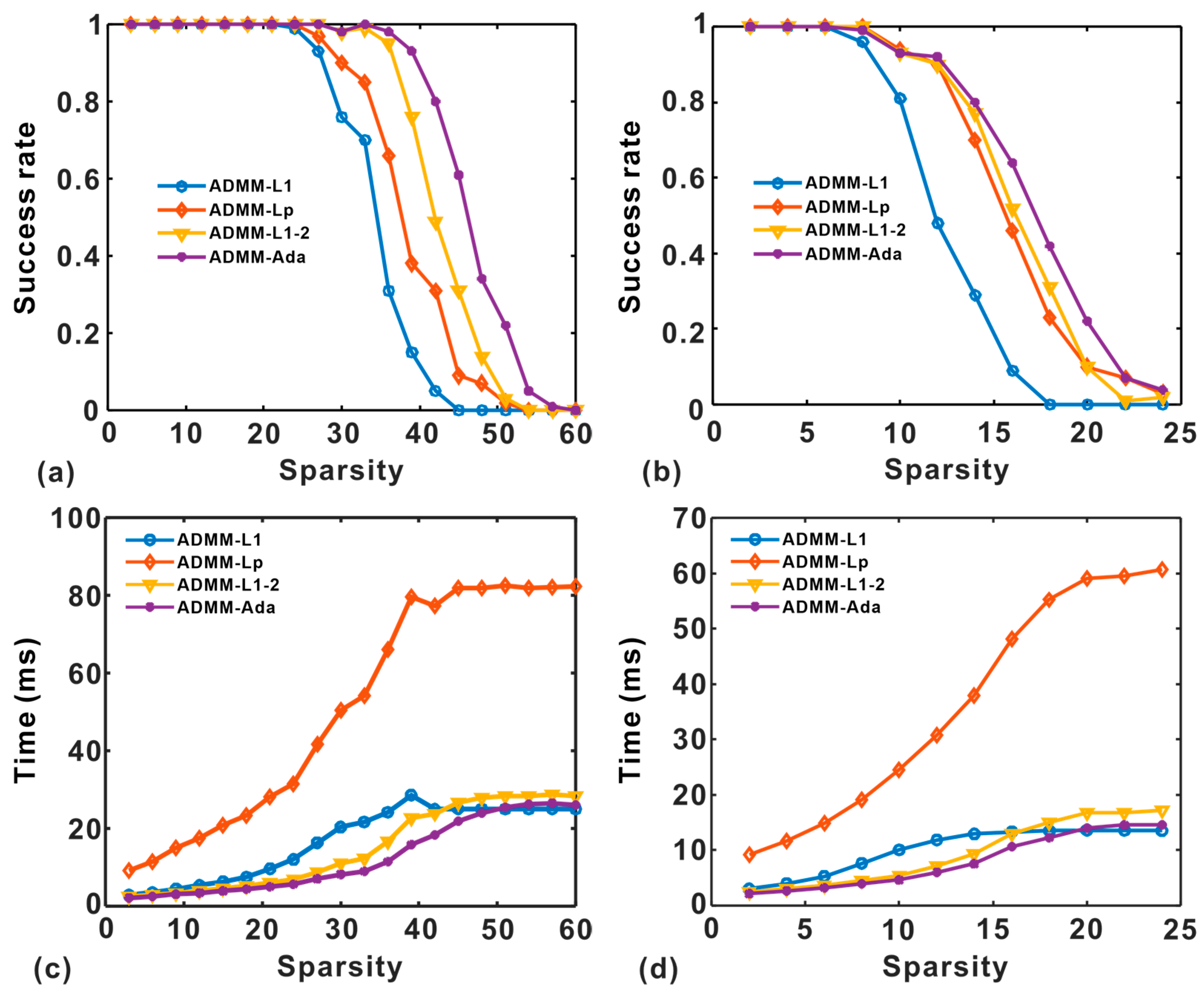
Under low-coherence conditions, with a Gaussian measurement matrix size of 128 × 512 and sparsity levels ranging from 3 to 60, the $L_1$ norm constraint regularization parameter was $3\times {10}^{-3}\times \Vert \mathit{x}{\Vert }_{\infty }$, the $L_{\mathrm{p}}$ quasi-norm $\Vert \mathit{x}{\Vert }_{0.5}$ regularization parameter was $5\times {10}^{-3}\times \Vert \mathit{x}{\Vert }_{\infty }$, the quasi-norm $\Vert \mathit{x}{\Vert }_1-3/2\Vert \mathit{x}{\Vert }_2$ regularization parameter was $5\times {10}^{-3}\times \Vert \mathit{x}{\Vert }_{\infty }$, and the inverse-weighted regularization $Ada\left[\mathit{x}\right]$ parameter was $5\times {10}^{-3}\times \Vert \mathit{x}{\Vert }_{\infty }$. Under strongly coherent conditions, with a Gaussian measurement matrix size of 64 × 512 and sparsity levels ranging from 2 to 24, the $L_1$ norm constraint regularization parameter was $3\times {10}^{-3}\times \Vert \mathit{x}{\Vert }_{\infty }$, the $L_{\mathrm{p}}$ quasi-norm $\Vert \mathit{x}{\Vert }_{0.5}$ regularization parameter was $8\times {10}^{-3}\times \Vert \mathit{x}{\Vert }_{\infty }$, the pseudo-norm $\Vert \mathit{x}{\Vert }_1-3/2\Vert \mathit{x}{\Vert }_2$ regularization parameter was $8\times {10}^{-3}\times \Vert \mathit{x}{\Vert }_{\infty }$, and the inverse-weighted regularization $Ada\left[\mathit{x}\right]$ parameter was $5\times {10}^{-3}\times \Vert \mathit{x}{\Vert }_{\infty }$. The number of iterations for the tested algorithms was 1000. The test results are depicted in Figure 1. In this testing model, for both strongly and weakly coherent Gaussian random measurement matrices, the reconstruction success rate using $Ada\left[\mathit{x}\right]$ as the sparse constraint surpassed that of the other norm constraints (Figure 1a,b). Figure 1c and Figure 1d respectively illustrate the average computational time of different algorithms with 1000 iterations for various sparsity levels under weakly and strongly coherent conditions. The results show that the computational time of the proposed algorithm is comparable to that of the other methods under both conditions, indicating that the proposed approach does not introduce a significant additional computational burden.

3.2. Natural Image Processing Test

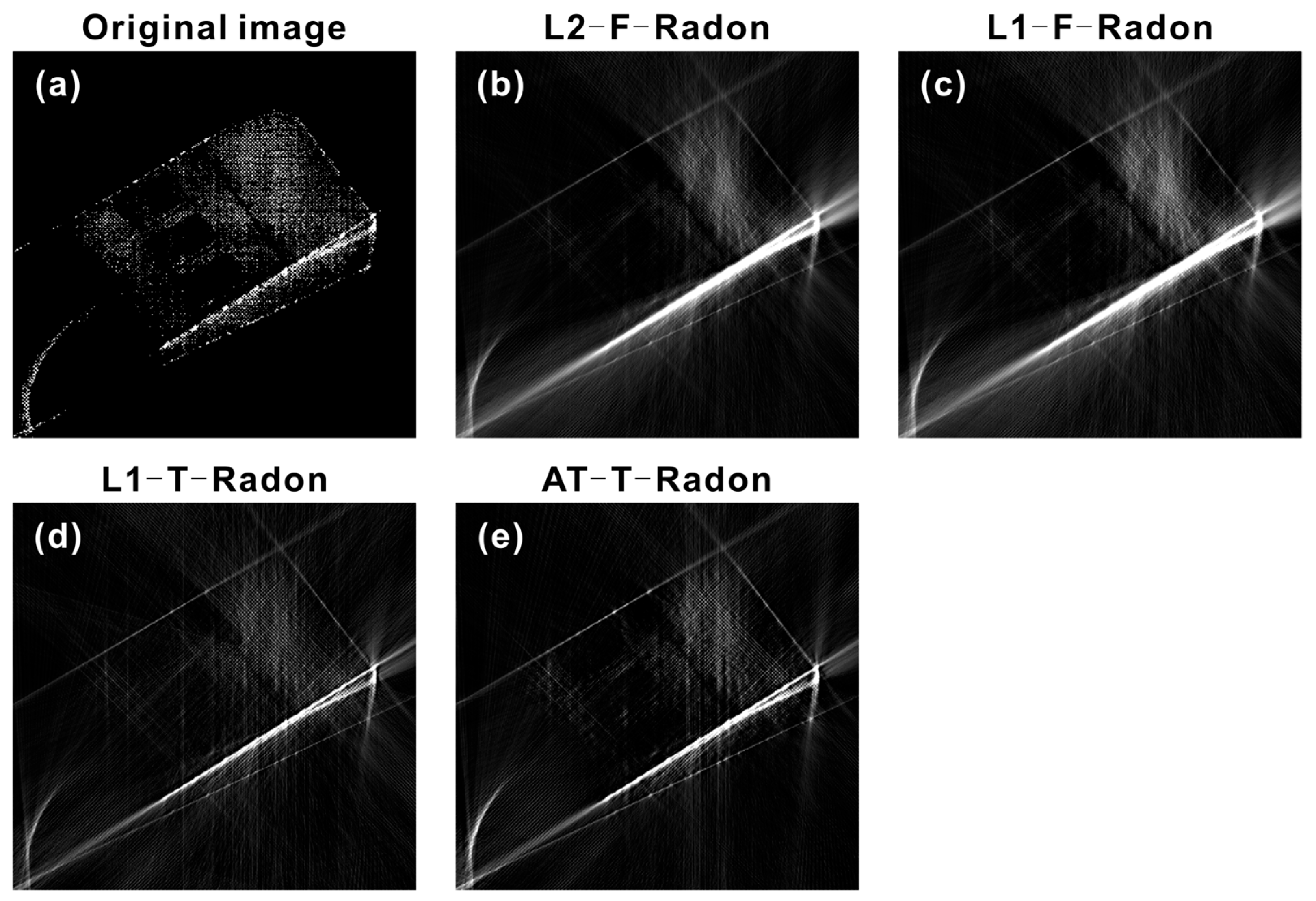
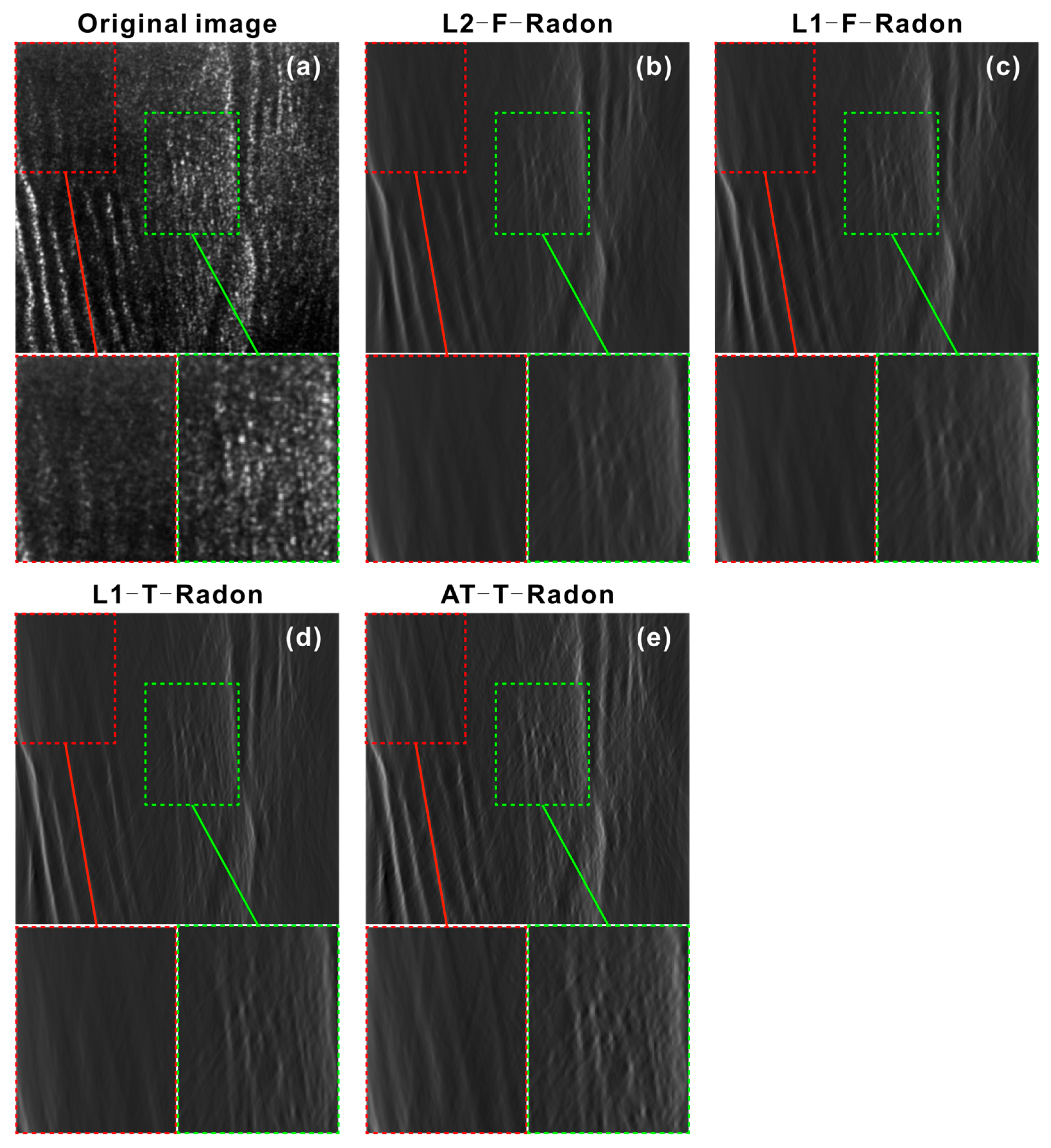
For the linear Radon transform, we conducted tests on the linear enhancement processing of natural images. The image test results are presented in Figure 2 and Figure 3, where Figure 2a and Figure 3a represent the original images, and Figure 2b–e and Figure 3b–e respectively utilize $L_2$ norm frequency domain Radon transform (L2-F-RT), $L_1$ norm frequency domain Radon transform (L1-F-RT), $L_1$ norm time domain Radon transform (L1-T-RT), and time domain inverse-weighted regularized Radon transform (AT-T-RT) for linear enhancement of the original images. Since the Radon transform is a global transformation, the inevitable energy leakage resulted in the phenomenon of line crossing. The application of spatial domain thresholds made linear features more prominent, resulting in clearer images. The test results indicate that the Radon transform with inverse-weighted regularization constraint performs better in image linear enhancement tests (Figure 2e and Figure 3e).

3.3. Test of Seismic Data Processing

In the processing of seismic data, effective suppression of multiples can provide reliable data for seismic imaging [44,45], seismic inversion [46] and reservoir inversion [47,48], the Radon transform with a parabolic trajectory is frequently employed to mitigate multiple reflections [49]. Its principle involves concentrating primary waves and multiple reflections at distinct curvatures within the Radon domain, facilitating the discernment and removal of energy clusters associated with multiple reflections. Subsequently, the data in the Radon domain transforms back into the time-space domain to provide a clear representation of the underground structure.

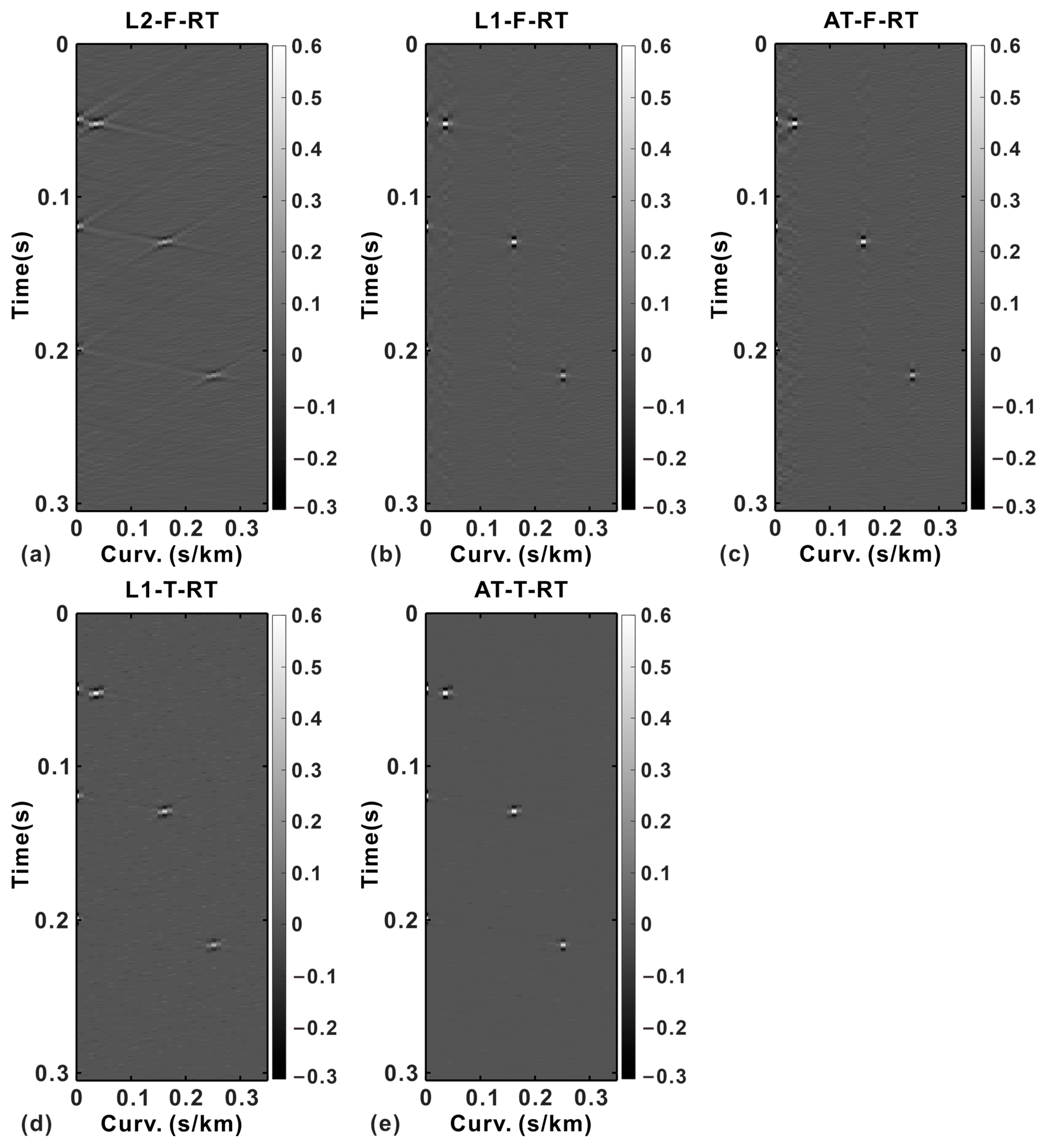
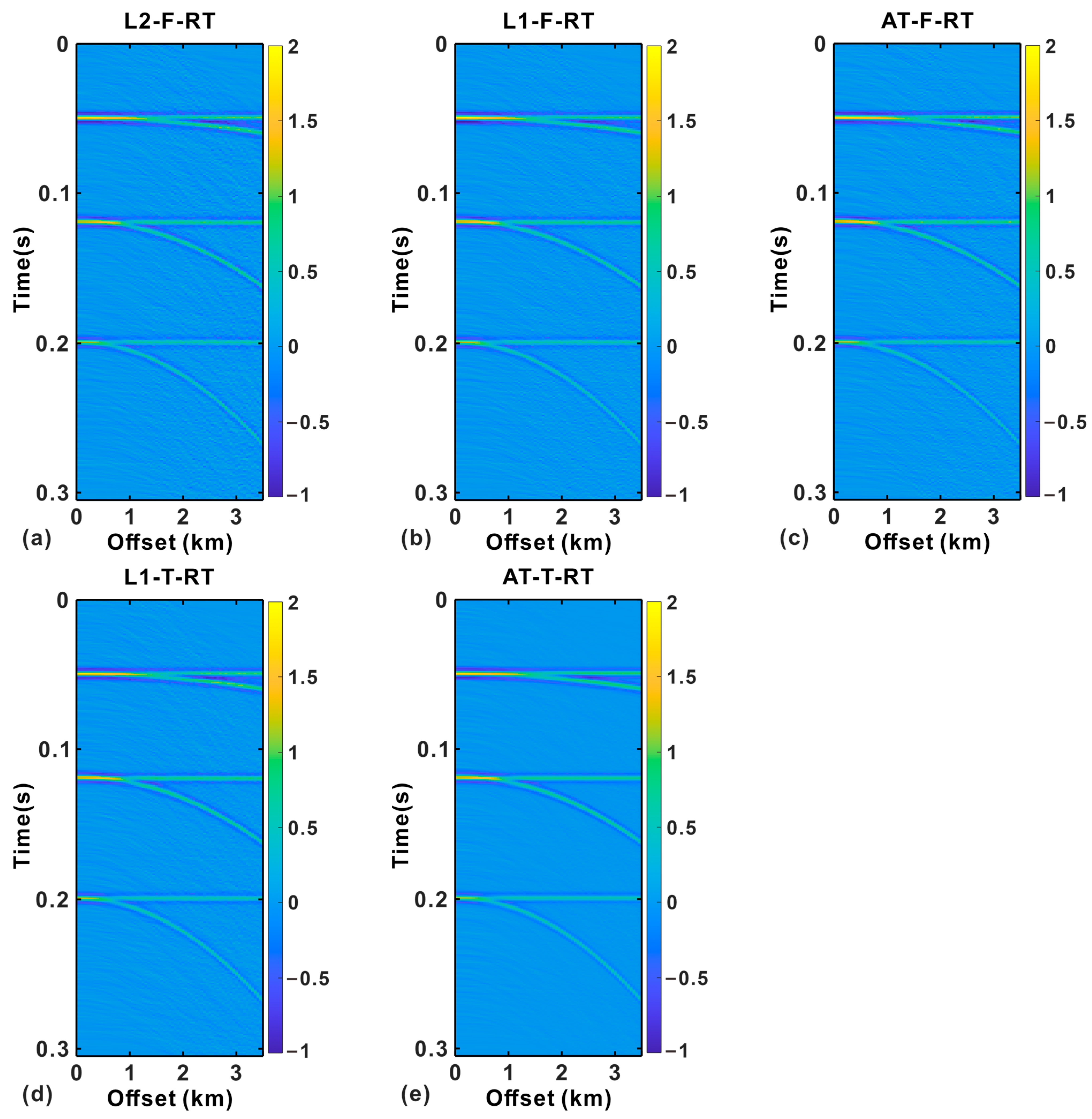
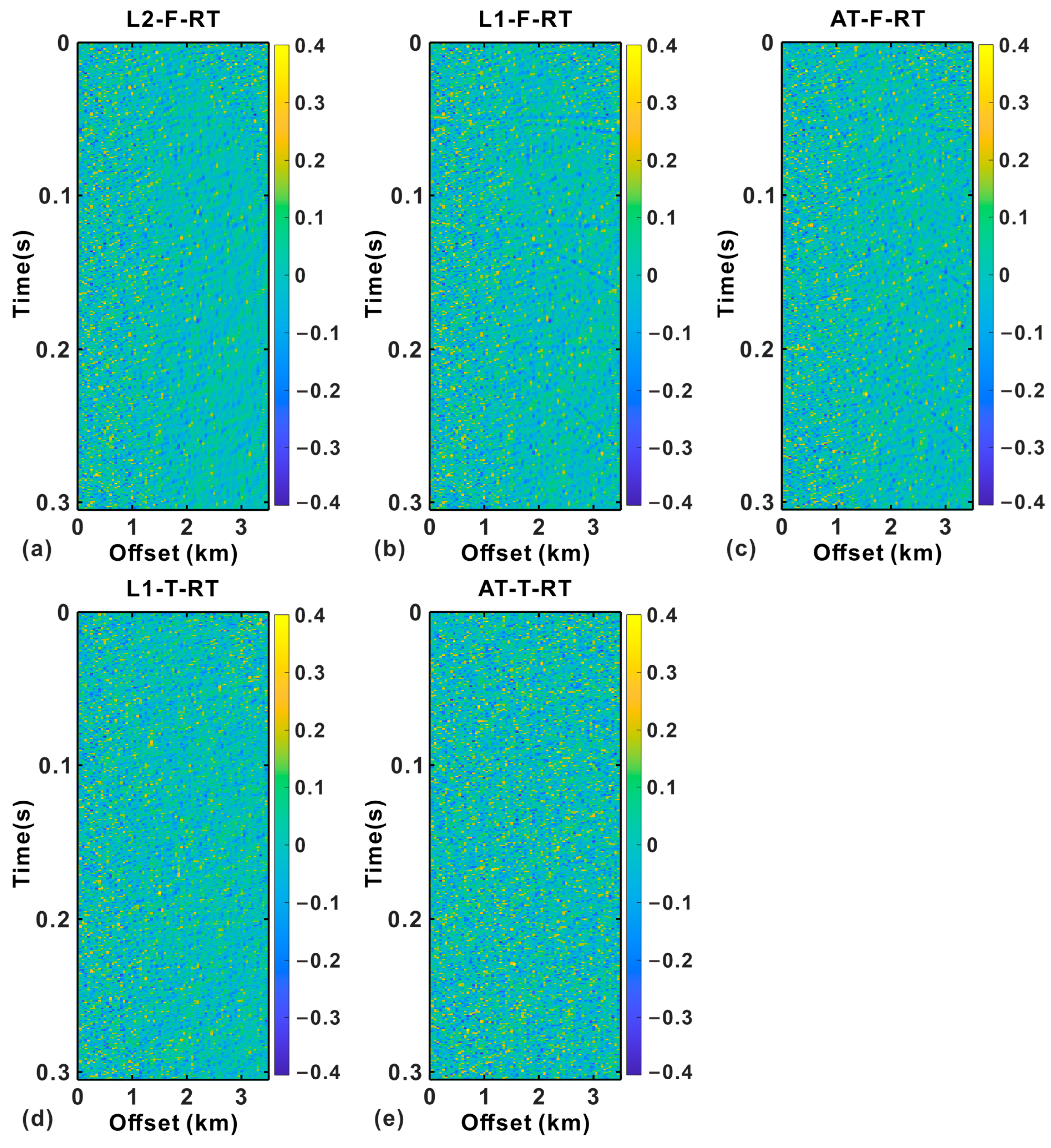
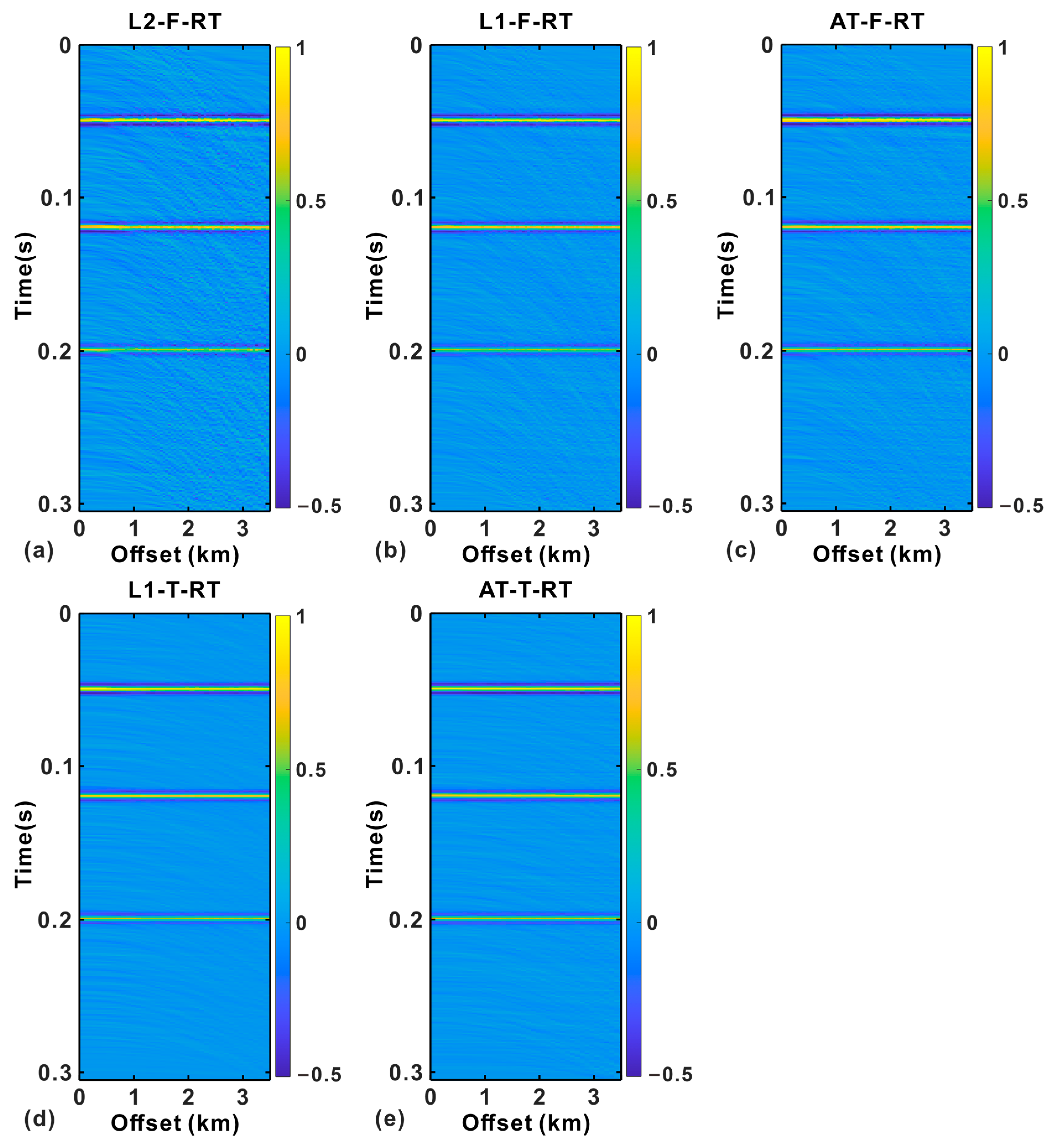
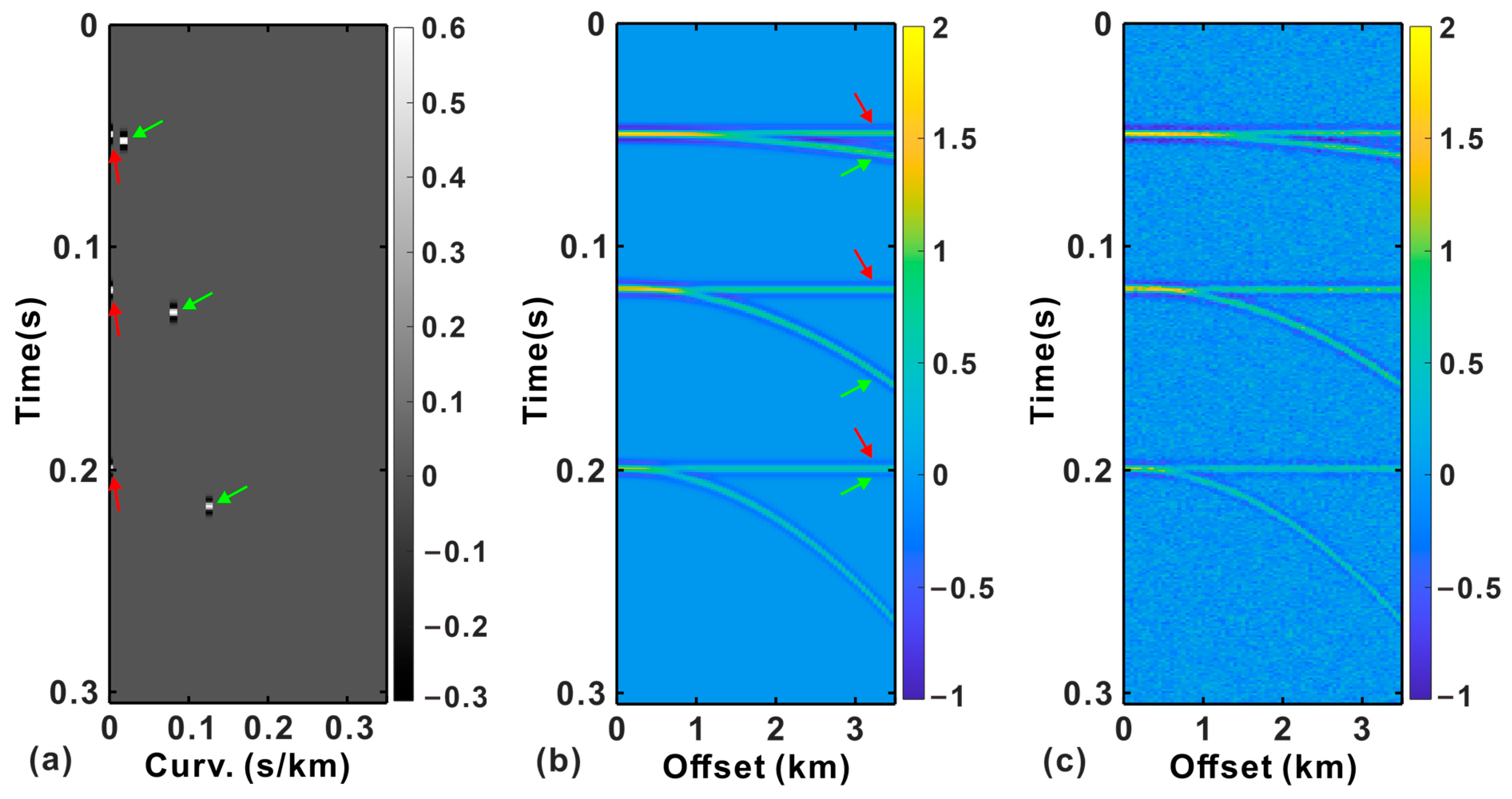
To validate the effectiveness of the proposed method, we simulated common midpoint point (CMP) gather data after normal moveout correction (Figure 4b) and added random noise to achieve a signal-to-noise ratio of 6.02 dB (Figure 4c). In the Radon domain, primary waves aggregated at zero curvature positions (red arrow in Figure 4a), and multiple reflections aggregated at large curvature positions (green arrow in Figure 4a). In the time domain, the primary wave manifested as a straight events axis (red arrow in Figure 4b), while multiple reflections were characterized by a curved events axis (green arrow in Figure 4b). Tests were conducted based on L2-F-RT, L1-F-RT, frequency domain inverse-weighted regularized Radon transform (AT-F-RT), L1-T-RT, and AT-T-RT. Figure 5 illustrates the Radon transform results from Figure 4b; Figure 6 presents the time-space domain data acquired through the inverse transformation of the Radon domain data in Figure 5; Figure 7 displays the variance between the forward and inverse Radon transform outcomes using different methods and the field model (Figure 4c); Figure 8 portrays the time-space domain data obtained after eliminating the energy clusters of multiple reflections in the Radon domain, to suppress these reflections.

For the $L_2$ norm-constrained Radon transform, L2-F-RT experienced energy tailing, which is disadvantageous for suppressing multiple reflections (Figure 5a, Figure 6a, Figure 7a and Figure 8a). The frequency domain sparse-constrained Radon transform algorithms (L1-F-RT and AT-F-RT) generated striped noise and exhibited a substantial error when transformed back into the time-space domain (Figure 5b, Figure 6b and Figure 7b). Although AT-F-RT showed some improvements on this basis (Figure 5c, Figure 6c and Figure 7c), it lost some effective signals, disqualifying it as a lossless transformation. In comparison to the frequency domain Radon transforms (Figure 7b,c), the time domain sparse-constraint Radon transforms (L1-T-RT and AT-T-RT) experienced less energy loss (Figure 7d,e), and AT-T-RT effectively enhanced the energy focusing of the transform domain (Figure 5d,e), thereby reducing the inverse transform error (Figure 6d,e and Figure 7d,e). Essentially, it successfully suppressed multiple reflections (Figure 8d,e).

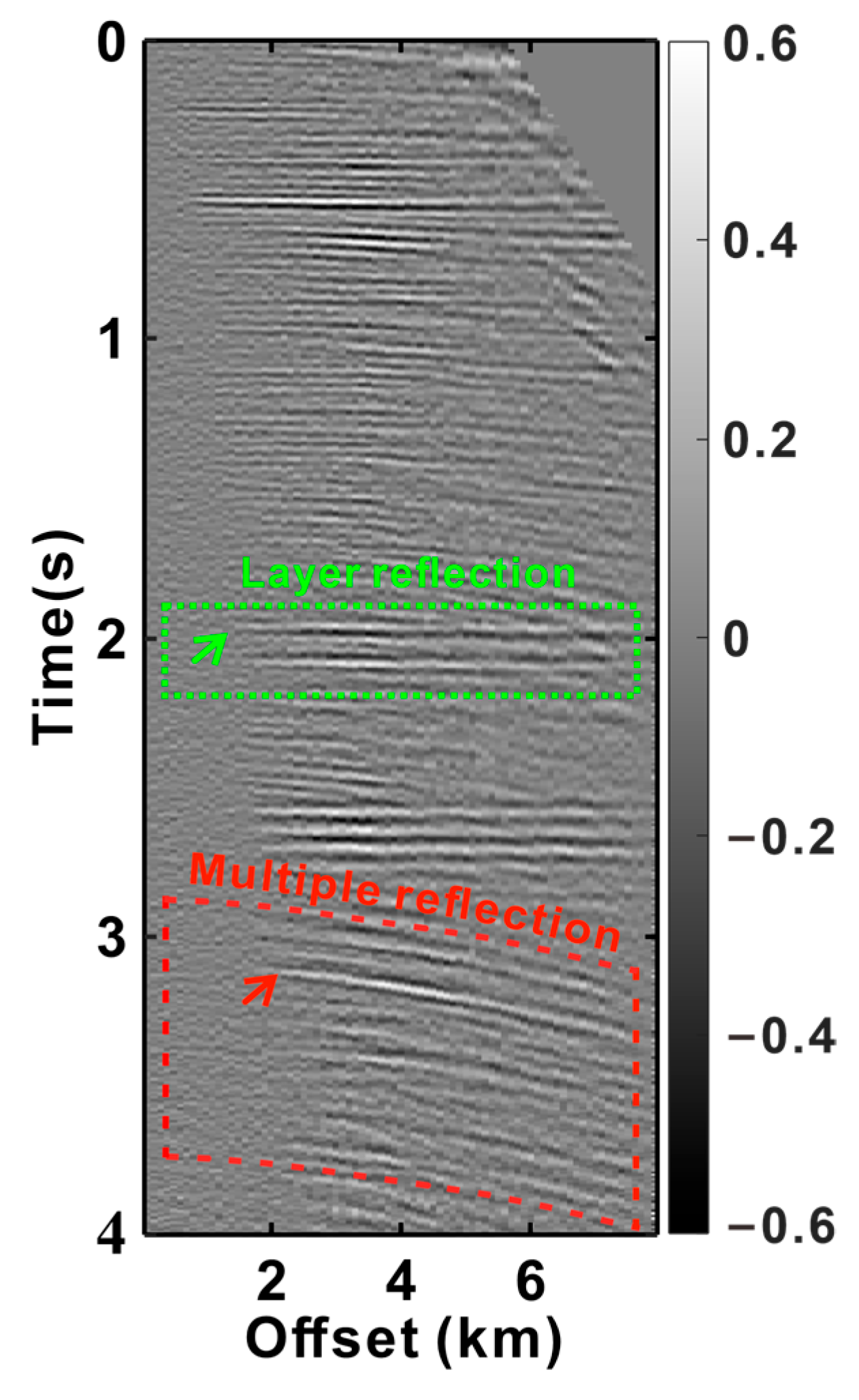
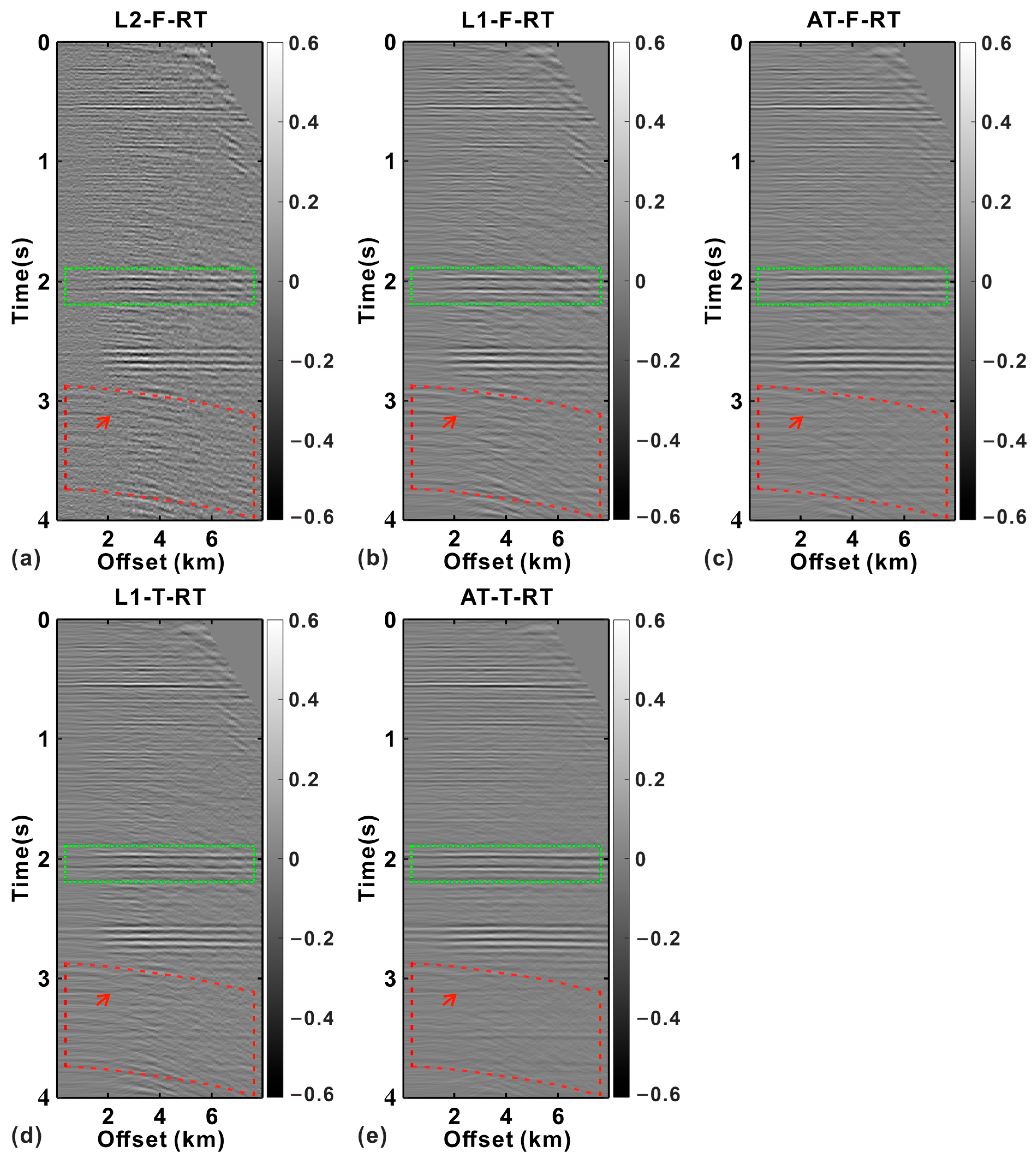
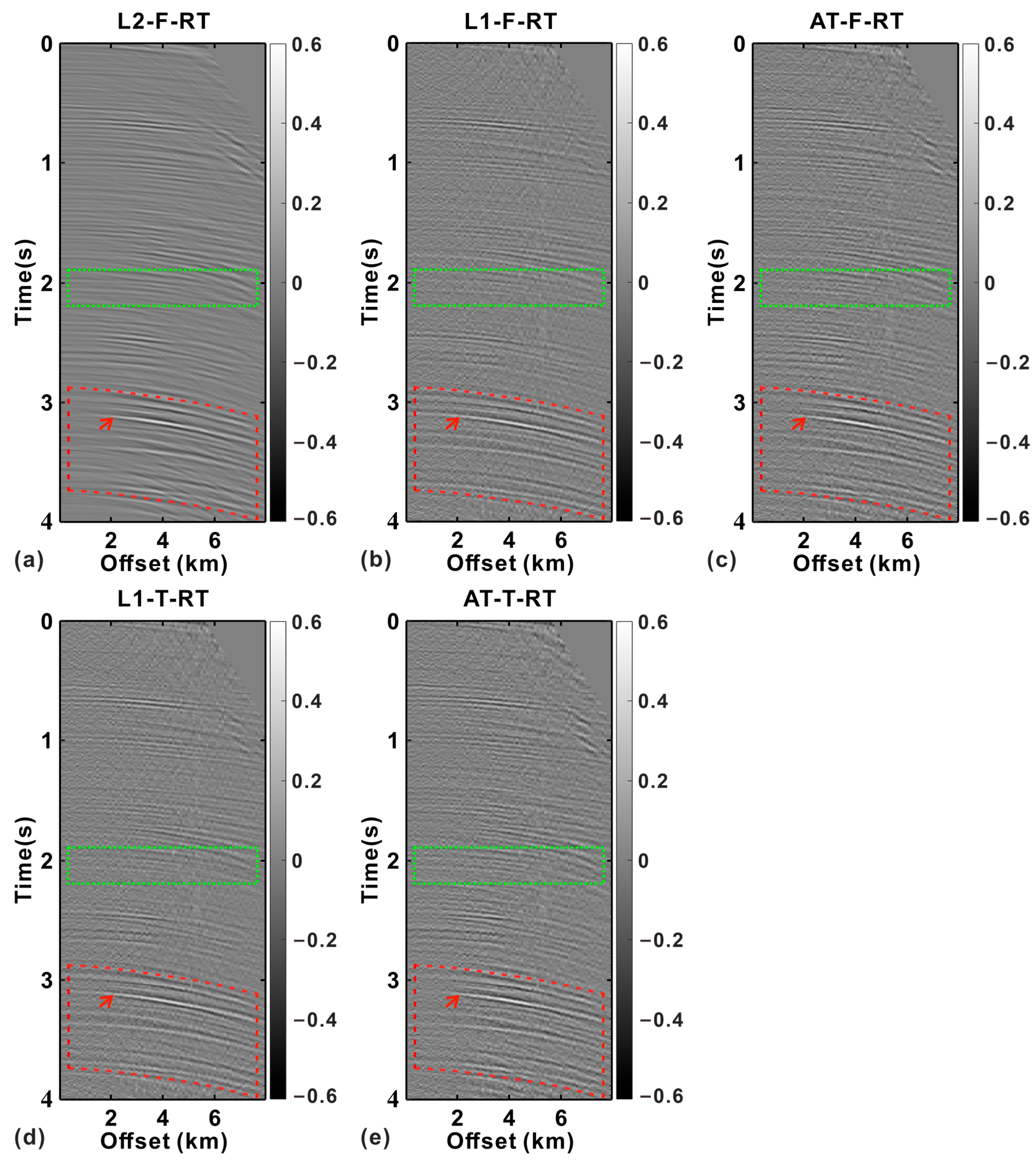
To validate the applicability of the proposed method in field data, we selected actual seismic data for testing. The data comprises CMP gather data after normal moveout correction (Figure 9), where the curvature of the primary wave is approximately zero, and the events axis is relatively straight (green dashed box), while the curvature of the events axis of the multiple waves is not zero, and there is residual time difference compared to the primary wave (red dashed box). We conducted tests using L2-F-RT, L1-F-RT, AT-F-RT, L1-T-RT, and AT-T-RT to suppress multiple reflections. Figure 10 presents the results after employing various algorithms to suppress multiple reflections, while Figure 11 illustrates the multiple reflection data removed using different methods. In Figure 10a, the result is obtained by applying muting operation. Comparing Figure 9 and Figure 11, efforts were made to preserve effective signals as much as possible in the calculations to minimize damage to the primary wave. From the calculation results (Figure 10 and Figure 11), it can be observed that, whether in the frequency domain Radon transform or time domain Radon transform, using the inverse-weighted regularization-constrained Radon transform could better suppress multiple reflections. This indicates that replacing conventional sparse constraints with the inverse-weighted regularization constraint can improve the ability of signal-noise separation in the Radon transform.

4. Conclusions

In this study, we examined the relationship between the mismatch term constraint and the regularization term. When the regularization weight is large, the mismatch term weight is small, leading to a suboptimal match with the observed data. Conversely, with a small regularization weight, the mismatch term weight becomes large, rendering the regularization term ineffective in constraining it. Hence, we introduced an adaptive threshold. Employing the inverse-weighted strategy, we utilized the inverse weighting of the sparse domain data. We posit that larger values in certain portions should have a proportionately larger mismatch term weight to ensure similarity with the observed data. Conversely, for regions with smaller values, a smaller mismatch term weight is employed to enhance the sparsity of the transform domain. Building on this principle, we apply it to the Radon transform and introduced the Radon transform with inverse-weighted regularization sparse constraint in both time and frequency domains. We applied this methodology to process natural images and seismic data. The results from both the model and real data demonstrated that our proposed algorithm effectively enhances the accuracy of sparse data reconstruction, increases sparsity constraint capability, and improves the application effectiveness of the Radon transform.

References

1. Donoho, D.L. Compressed sensing. IEEE Trans. Inf. Theory 2006, 52, 1289–1306. [Google Scholar] [CrossRef]
2. Duarte, M.F.; Davenport, M.A.; Takhar, D.; Laska, J.N.; Sun, T.; Kelly, K.F.; Baraniuk, R.G. Single-pixel imaging via compressive sampling. IEEE Signal Process. Mag. 2008, 25, 83–91. [Google Scholar] [CrossRef]
3. Lustig, M.; Donoho, D.; Pauly, J.M. Sparse MRI: The application of compressed sensing for rapid MR imaging. Magn. Reson. Med. 2007, 58, 1182–1195. [Google Scholar] [CrossRef]
4. Berger, C.R.; Zhou, S.; Preisig, J.C.; Willett, P. Sparse channel estimation for multicarrier underwater acoustic communication: From subspace methods to compressed sensing. IEEE Trans. Signal Process. 2009, 58, 1708–1721. [Google Scholar] [CrossRef]
5. Gan, S.; Wang, S.; Chen, Y.; Chen, X.; Huang, W.; Chen, H. Compressive sensing for seismic data reconstruction via fast projection onto convex sets based on seislet transform. J. Appl. Geophys. 2016, 130, 194–208. [Google Scholar] [CrossRef]
6. Candes, E.J.; Wakin, M.B.; Boyd, S.P. Enhancing sparsity by reweighted L1 minimization. J. Fourier Anal. Appl. 2008, 14, 877–905. [Google Scholar] [CrossRef]
7. Shen, C.; Wang, G.; Liu, L.; Ren, D.; Hu, H.; Sun, W. Extraction of periodic terms in satellite clock bias based on Fourier basis pursuit bandpass filter. Remote Sens. 2025, 17, 827. [Google Scholar] [CrossRef]
8. Chen, S.; Cao, S.; Sun, Y. Resolution-oriented weighted stacking algorithm. IEEE Trans. Geosci. Remote Sens. 2022, 60, 5914407. [Google Scholar] [CrossRef]
9. Foucart, S.; Rauhut, H. A Mathematical Introduction to Compressive Sensing. Bull. Am. Math. 2017, 54, 151–165. [Google Scholar] [CrossRef]
10. Ge, D.; Jiang, X.; Ye, Y. A note on the complexity of Lp minimization. Math. Program. 2011, 129, 285–299. [Google Scholar] [CrossRef]
11. Yin, P.; Lou, Y.; He, Q.; Xin, J. Minimization of L1–2 for compressed sensing. SIAM J. Sci. Comput. 2015, 37, A536–A563. [Google Scholar] [CrossRef]
12. Cai, Y. Weighted Lp–L1 minimization methods for block sparse recovery and rank minimization. Anal. Appl. 2021, 19, 343–361. [Google Scholar] [CrossRef]
13. Wang, D. Spectral L2/L1 norm: A new perspective for spectral kurtosis for characterizing non-stationary signals. Mech. Syst. Signal Process. 2018, 104, 290–293. [Google Scholar] [CrossRef]
14. Chen, S.; Donoho, D.L.; Saunders, M.A. Atomic decomposition by basis pursuit. SIAM Rev. 2001, 43, 129–159. [Google Scholar] [CrossRef]
15. Calamai, P.H.; Moré, J.J. Projected gradient methods for linearly constrained problems. Math. Program. 1987, 39, 93–116. [Google Scholar] [CrossRef]
16. Gubin, L.G.; Polyak, B.T.; Raik, E.V. The method of projections for finding the common point of convex sets. USSR Comput. Math. Math. Phys. 1967, 7, 1–24. [Google Scholar] [CrossRef]
17. Bredies, K.; Lorenz, D.A. Linear convergence of iterative soft-thresholding. J. Fourier Anal. Appl. 2008, 14, 813–837. [Google Scholar] [CrossRef]
18. Blumensath, T.; Davies, M.E. Iterative hard thresholding for compressed sensing. Appl. Comput. Harmon. Anal. 2009, 27, 265–274. [Google Scholar] [CrossRef]
19. Natarajan, B.K. Sparse approximate solutions to linear systems. SIAM J. Comput. 1995, 24, 227–234. [Google Scholar] [CrossRef]
20. Feng, M.; Mitchell, J.E.; Pang, J.S.; Shen, X.; Wächter, A. Complementarity formulations of L0-norm optimization problems. Pac. J. Optim. 2018, 14, 273–305. [Google Scholar]
21. Yang, J.; Wright, J.; Huang, T.S.; Ma, Y. Image super-resolution via sparse representation. IEEE Trans. Image Process. 2010, 19, 2861–2873. [Google Scholar] [CrossRef]
22. Wang, J.; Lu, H.; Liang, Z.; Eremina, D.; Zhang, G.; Wang, S.; Chen, J.; Manzione, J. An experimental study on the noise properties of x-ray CT sinogram data in Radon space. Phys. Med. Biol. 2008, 53, 3327–3341. [Google Scholar] [CrossRef] [PubMed]
23. Ma, J.; Xu, G.; Chen, X.; Wang, X.; Hao, Z. Multiple attenuation with 3D high-order high-resolution parabolic Radon transform using lower frequency constraints. Geophysics 2020, 85, V317–V328. [Google Scholar] [CrossRef]
24. Chen, S.; Wang, N.; Shi, Y.; Guo, M.X.; Shi, W.; Cao, S.Y.; Jin, Z.Q. Sparse Gabor Transform and its application in seismic data analysis. IEEE Trans. Geosci. Remote Sens. 2025, 63, 5911210. [Google Scholar] [CrossRef]
25. Daubechies, I. The wavelet transform, time-frequency localization and signal analysis. IEEE Trans. Inf. Theory 1990, 36, 961–1005. [Google Scholar] [CrossRef]
26. Ahmed, N.; Natarajan, T.; Rao, K.R. Discrete cosine transform. IEEE Trans. Comput. 1974, C-23, 90–93. [Google Scholar] [CrossRef]
27. Beylkin, G. Discrete Radon transform. IEEE Trans. Acoust. Speech Signal Process. 1987, 35, 162–172. [Google Scholar] [CrossRef]
28. Seo, J.S.; Haitsma, J.; Kalker, T.; Yoo, C.D. A robust image fingerprinting system using the Radon transform. Signal Process. Image Commun. 2004, 19, 325–339. [Google Scholar] [CrossRef]
29. Xue, Y.; Ma, J.; Chen, X. High-order sparse Radon transform for AVO-preserving data reconstruction. Geophysics 2014, 79, V13–V22. [Google Scholar] [CrossRef]
30. Shi, Y.; Wang, W.H. Surface-related multiple suppression approach by combining wave equation prediction and hyperbolic Radon transform. Chin. J. Geophys. 2012, 55, 3115–3125. [Google Scholar] [CrossRef]
31. Geng, W.; Li, J.; Chen, X.; Ma, J.; Xu, J.; Zhu, G.; Tang, W. 3D high-order sparse Radon transform with L1–2 minimization for multiple attenuation. Geophys. Prospect. 2022, 70, 655–676. [Google Scholar] [CrossRef]
32. Ma, J.; Zhao, K.; Liao, Z. A fast amplitude preserving three-parameter 3D parabolic Radon transform and its application on multiple attenuation. Pet. Sci. 2025, 22, 163–177. [Google Scholar] [CrossRef]
33. Feng, L.; Xue, Y.; Chen, C.; Su, J.; Zhang, C. An efficient amplitude-preserving Radon transform with frequency-dependent curvature for multiple attenuation. IEEE Trans. Geosci. Remote Sens. 2024, 62, 5904313. [Google Scholar] [CrossRef]
34. Xie, J.; Wang, X.; Wang, X.; Dun, S.; Zeng, H.; Jin, B. Multiple-suppression method using the λ-f domain high-resolution parabolic Radon transform with curvature magnification. Appl. Geophys. 2024, 21, 169–178. [Google Scholar] [CrossRef]
35. Guo, M.; Chen, S.; Shi, W.; Wang, W. A Radon-domain sparsity enhancement algorithm based on 3D deconvolution. Geophys. Prospect. Pet. 2026, 65, 224–233. [Google Scholar] [CrossRef]
36. Shi, W.; Wang, W.; Shi, Y.; Chen, S.; Li, Z.; Wang, N. 3D high-resolution Radon transform based on a strong sparse Lp–1 norm and its applications. J. Geophys. Eng. 2024, 21, 1008–1026. [Google Scholar] [CrossRef]
37. Sacchi, M.D.; Ulrych, T.J. High-resolution velocity gathers and offset space reconstruction. Geophysics 1995, 60, 1169–1177. [Google Scholar] [CrossRef]
38. Ouyang, Z.; Zhang, L.; Wang, H.; Yang, K. High-dimensional seismic data reconstruction based on linear Radon transform–constrained tensor CANDECOM/PARAFAC decomposition. Remote Sens. 2022, 14, 6275. [Google Scholar] [CrossRef]
39. Wang, Y.; Gong, X.; Hu, B. Seismic data reconstruction using a phase-shift-plus-interpolation-based apex-shifted hyperbolic Radon transform. Remote Sens. 2024, 16, 1114. [Google Scholar] [CrossRef]
40. Su, Y.; Wang, D.; Hu, B.; Gong, X.; Zhang, J. Supervirtual refraction interferometry in the Radon domain. Remote Sens. 2023, 15, 384. [Google Scholar] [CrossRef]
41. Biondi, F. Low-rank plus sparse decomposition and localized Radon transform for ship-wake detection in synthetic aperture radar images. IEEE Geosci. Remote Sens. Lett. 2018, 15, 117–121. [Google Scholar] [CrossRef]
42. Parikh, N.; Boyd, S. Proximal algorithms. Found. Trends Optim. 2014, 1, 127–239. [Google Scholar] [CrossRef]
43. Boyd, S.; Parikh, N.; Chu, E.; Peleato, B.; Eckstein, J. Distributed optimization and statistical learning via the alternating direction method of multipliers. Found. Trends Mach. Learn. 2011, 3, 1–122. [Google Scholar] [CrossRef]
44. Xu, Q.; Wang, Y. Seismic reverse time migration based on biaxial wavefield decomposition. Geophysics 2024, 89, S61–S70. [Google Scholar] [CrossRef]
45. Zhang, W.; Ravasi, M.; Gao, J.; Shi, Y. Deep-unrolling architecture for image-domain least-squares migration. Geophysics 2024, 89, S215–S234. [Google Scholar] [CrossRef]
46. Pan, X.; Zhao, Z. A decoupled fracture- and stress-induced PP-wave reflection coefficient approximation for azimuthal seismic inversion in stressed horizontal transversely isotropic media. Surv. Geophys. 2024, 45, 151–182. [Google Scholar] [CrossRef]
47. Shi, Y.; Yu, B.; Zhou, H.; Cao, Y.; Wang, W.; Wang, N. FMG_INV, a fast multi-Gaussian inversion method integrating well-log and seismic data. IEEE Trans. Geosci. Remote Sens. 2024, 62, 4503112. [Google Scholar] [CrossRef]
48. Wang, N.; Liu, W.; Shi, Y.; Li, S.L.; Li, Y. Q-Compensated full waveform inversion based on constant-fractional explicit stable compensated equation. IEEE Trans. Geosci. Remote Sens. 2025, 63, 5926214. [Google Scholar] [CrossRef]
49. Hampson, D. Inverse velocity stacking for multiple elimination. In SEG Technical Program Expanded Abstracts; Society of Exploration Geophysicists: Houston, TX, USA, 1986; pp. 422–424. [Google Scholar] [CrossRef]
Figure 1. Sparse reconstruction probability and the computational cost. (a) Weakly correlated Gaussian random measurement array; (b) Strongly correlated Gaussian random measurement array; (c) Time cost under the weakly coherent conditions; (d) Time cost under the strongly coherent conditions.
Remotesensing 18 01834 g001
Figure 2. Linear enhancement model test. (a) Original image; (b) Result obtained using L 2  norm frequency domain Radon transform (L2-F-RT); (c) Result obtained using L 1  norm frequency domain Radon transform (L1-F-RT); (d) Result obtained using L 1  norm time domain Radon transform (L1-T-RT); (e) Result obtained using time domain inverse-weighted regularized Radon transform (AT-T-RT).
Remotesensing 18 01834 g002
Figure 3. Linear enhancement test on natural images. (a) Original image; (b) Result obtained using L 2  norm frequency domain Radon transform (L2-F-RT); (c) Result obtained using L 1  norm frequency domain Radon transform (L1-F-RT); (d) Result obtained using L 1  norm time domain Radon transform (L1-T-RT); (e) Result obtained using time domain inverse-weighted regularized Radon transform (AT-T-RT).
Remotesensing 18 01834 g003
Figure 4. Model data. (a) τ p  domain data; (b) Synthetic noise-free CMP gather; (c) CMP gather with added random noise.
Remotesensing 18 01834 g004
Figure 5. Radon domain data calculated by different methods. (a) L 2  norm frequency domain Radon transform (L2-F-RT); (b) L 1  norm frequency domain Radon transform (L1-F-RT); (c) Frequency domain inverse-weighted regularized Radon transform (AT-F-RT); (d) L 1  norm time domain Radon transform (L1-T-RT); (e) Time domain inverse-weighted regularized Radon transform (AT-T-RT).
Remotesensing 18 01834 g005
Figure 6. t-x domain data obtained by inverse transform from Figure 5. (a) Result from L2-F-RT; (b) Result from L1-F-RT; (c) Result from AT-F-RT; (d) Result from L1-T-RT; (e) Result from AT-T-RT.
Remotesensing 18 01834 g006
Figure 7. Difference between Figure 4c and Figure 6. (a) Difference for L2-F-RT; (b) Difference for L1-F-RT; (c) Difference for AT-F-RT; (d) Difference for L1-T-RT; (e) Difference for AT-T-RT.
Remotesensing 18 01834 g007
Figure 8. Results after suppressing multiple reflections by different methods. (a) Result using L2-F-RT; (b) Result using L1-F-RT; (c) Result using AT-F-RT; (d) Result using L1-T-RT; (e) Result using AT-T-RT.
Remotesensing 18 01834 g008
Figure 9. Field data.
Remotesensing 18 01834 g009
Figure 10. Data after suppressing multiple reflections. (a) Result using L2-F-RT; (b) Result using L1-F-RT; (c) Result using AT-F-RT; (d) Result using L1-T-RT; (e) Result using AT-T-RT.
Remotesensing 18 01834 g010
Figure 11. Suppressed multiple reflections. (a) Suppressed component using L2-F-RT; (b) Suppressed component using L1-F-RT; (c) Suppressed component using AT-F-RT; (d) Suppressed component using L1-T-RT; (e) Suppressed component using AT-T-RT.
Remotesensing 18 01834 g011
Disclaimer/Publisher’s Note: The statements, opinions and data contained in all publications are solely those of the individual author(s) and contributor(s) and not of MDPI and/or the editor(s). MDPI and/or the editor(s) disclaim responsibility for any injury to people or property resulting from any ideas, methods, instructions or products referred to in the content.