Comparative Evaluation of Machine Learning Models for Satellite Chlorophyll-a Gap Reconstruction in the Chesapeake Bay

Highlights

What are the main findings?

• Machine learning, deep learning, and convolutional autoencoder approaches can effectively reconstruct missing chlorophyll-a values in cloud-affected Sentinel-3 satellite data.
• XGBoost achieved the highest reconstruction accuracy (R² ≈ 0.86) among the tested models (IDW, KNN, DINEOF, DINCAE, RF, Extra Trees, XGBoost, and LSTM).
• Ensemble models better capture nonlinear seasonal bloom dynamics

What are the implications of the main findings?

• Gap-filled datasets improve the continuity of satellite-based HAB monitoring.
• The framework can support other reliable coastal water-quality monitoring.

Abstract

Harmful algal blooms (HABs) are increasing in frequency in the Chesapeake Bay, posing risks to marine ecosystems, water quality, and public health. Chlorophyll-a (Chl-a) is a widely used indicator of algal biomass, and satellite observations such as Sentinel-3 Ocean and Land Color Instrument (OLCI) enable large-scale monitoring of bloom dynamics. However, cloud cover and atmospheric interference frequently introduce missing pixels in daily satellite products, reducing temporal continuity and limiting monitoring reliability. Satellite-derived chlorophyll-a (Chl-a) data exhibit substantial missingness, with daily pixel gaps ranging from approximately 52.30% to 100% (mean ≈ 88.95%). This study evaluates spatial interpolation, EOF-based, supervised machine-learning, deep-learning, and convolutional autoencoder approaches for reconstructing missing Chl-a values. Sentinel-3 OLCI Chl-a data from 2023–2024 were used for model training, while data from 2025 served as a temporally independent test set to avoid spatiotemporal leakage. To simulate cloud-induced data gaps, artificial missingness scenarios ranging from 50% to 90% were applied for the Inverse Distance Weighting (IDW) and Data Interpolating Empirical Orthogonal Functions (DINEOF) baseline approaches, while machine-learning, deep-learning, and convolutional autoencoder models were evaluated using real satellite-derived missing observations. The evaluated models include IDW, DINEOF, K-Nearest Neighbors (KNN), Random Forest (RF), Extra Trees (ET), XGBoost, a Long Short-Term Memory (LSTM) network, and a Temporal Data Interpolating Convolutional Autoencoder (Temporal DINCAE). Model performance was assessed using Root Mean Square Error (RMSE), Mean Absolute Error (MAE), prediction bias, and the coefficient of determination (R²). Results indicate that tree-based ensemble models outperform spatial interpolation and EOF-based methods, with XGBoost achieving the best overall performance (R² ≈ 0.86; RMSE ≈ 9.61 mg m⁻³). The LSTM model achieved lower prediction errors (RMSE ≈ 5.87 mg m⁻³; MAE ≈ 2.16 mg m⁻³), highlighting the benefit of incorporating temporal dependencies, although with slightly reduced variance capture. The convolutional autoencoder-based Temporal DINCAE model achieved strong reconstruction performance (R² ≈ 0.84; RMSE ≈ 11.15 mg m⁻³). Uncertainty quantification shows that Extra Trees tends to underestimate uncertainty with narrower prediction intervals, whereas XGBoost provides better-calibrated but wider intervals.

1. Introduction

Harmful algal blooms (HABs) have emerged as a significant environmental concern in coastal and estuarine waters due to their ability to rapidly degrade water quality and disrupt aquatic ecosystems [1]. HAB events are typically associated with excessive phytoplankton growth, which reduces water clarity, limits light penetration to submerged vegetation, and contributes to oxygen depletion during bloom decay [2]. Certain bloom-forming species may also produce toxins, posing risks to marine organisms, fisheries, and public health through contaminated seafood [3]. Because bloom dynamics can evolve rapidly and exhibit strong spatial variability, reliability and continuous monitoring are essential for early detection and timely water-quality management. Chlorophyll-a (Chl-a), a photosynthetic pigment present in phytoplankton, is widely used as an indicator of algal biomass and HAB-related activity [4]. Elevated Chl-a concentrations often signal intensified phytoplankton presence and can help identify areas experiencing active or developing blooms. In estuarine systems such as the Chesapeake Bay—where nutrient inputs, freshwater inflow, and hydrodynamic processes vary substantially across space—Chl-a measurements provide an effective means of tracking bloom patterns at regional scales [5]. Continuous monitoring of Chl-a therefore plays a critical role in understanding bloom development and supporting HAB-related water-quality assessment.

In situ observations are commonly used to monitor HAB conditions by directly measuring Chl-a concentrations at discrete sampling locations [6]. These measurements, collected through water sampling or in-water sensors, are considered highly reliable and often serve as validation references in scientific studies [7]. However, in situ monitoring is inherently limited in spatial and temporal coverage. Observations represent specific points rather than continuous surfaces, leaving large areas unmeasured between stations. Field sampling also requires substantial logistical effort and resources, restricting measurement frequency and limiting the ability to capture rapidly evolving bloom dynamics. Because HAB events may intensify within days and vary considerably across short distances [8], reliance solely on periodic field observations is insufficient for comprehensive spatial–temporal characterization. Satellite remote sensing offers a complementary and scalable approach for HAB monitoring by providing repeated, synoptic coverage over extensive coastal regions [9]. Satellite missions such as Moderate Resolution Imaging Spectroradiometer (MODIS) and Visible Infrared Imaging Radiometer Suite (VIIRS) have been widely used for large-scale ocean and coastal observation [10]. Satellite-derived Chl-a products enable detection of spatial gradients across nearshore waters, tributary-influenced zones, and offshore regions where algal conditions can change rapidly [11]. Nevertheless, satellite monitoring in estuarine environments faces challenges due to atmospheric interference and optically complex waters that can affect retrieval accuracy [12]. Cloud cover remains one of the most persistent limitations, frequently obscuring the surface and creating missing values in daily Chl-a products [13]. These data gaps reduce temporal continuity and limit the reliability of bloom monitoring.

Improving the completeness of satellite-derived Chl-a datasets through gap-filling is therefore essential for enhancing operational monitoring capacity [14]. Machine-learning, deep-learning, and convolutional autoencoder approaches provide a flexible framework for estimating missing values by learning spatial and temporal patterns from available observations [14]. By leveraging historical data and contextual features, these models can reconstruct cloud-obscured regions while preserving environmental variability. The primary objective of this study is to identify an effective supervised learning framework for Chl-a gap reconstruction that improves satellite-based HAB monitoring and supports more reliable assessment of bloom dynamics in estuarine systems.

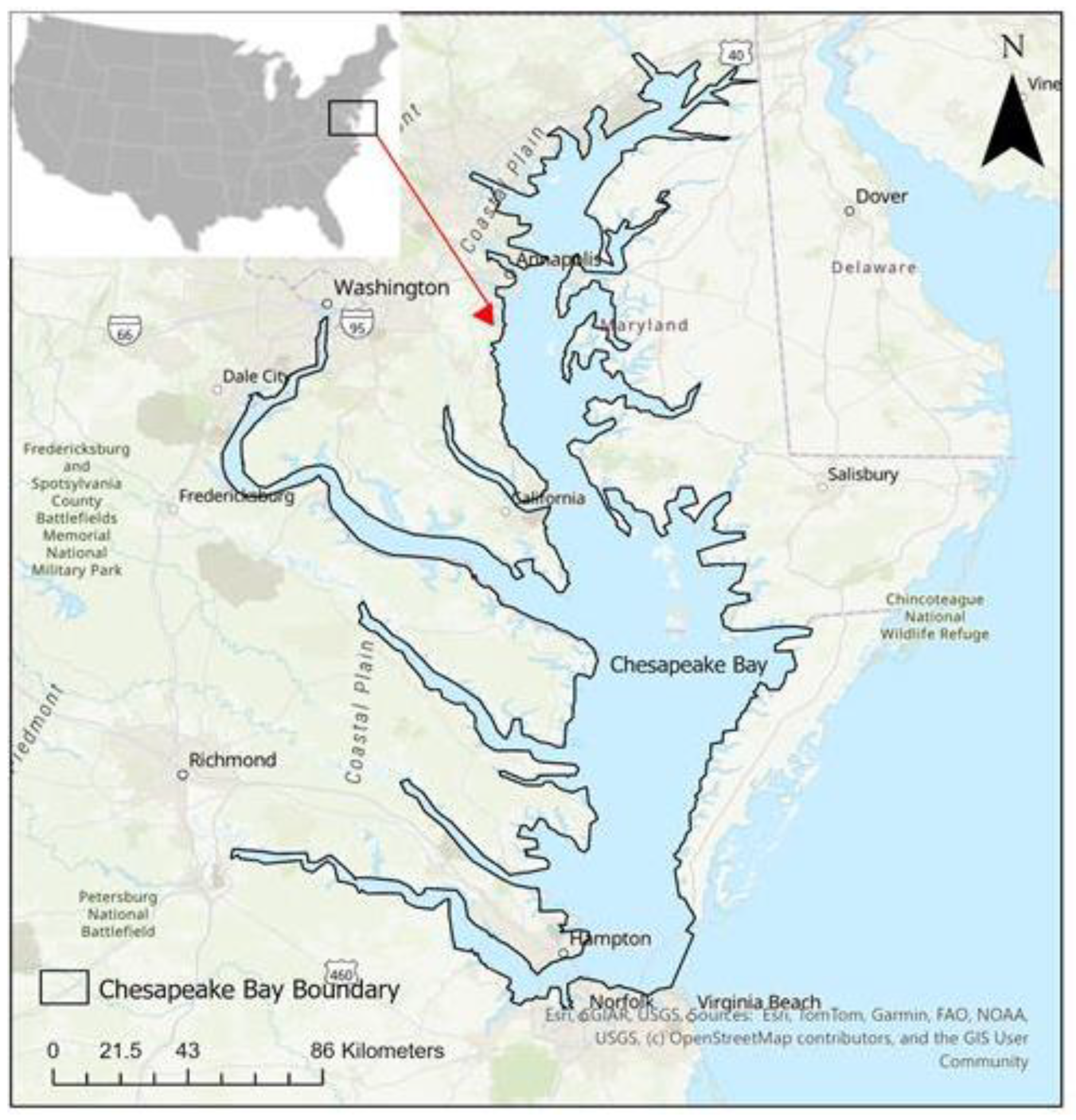
The remainder of this paper is organized as follows. Section Related Work reviews related research to establish methodological background and defines the research objectives. Section 2 describes the study area and provides geographic and environmental context. Section 3 presents the datasets used in this work, and Section 4 details the methodological framework adopted for Chl-a gap reconstruction and evaluation. Section 5 presents the results of the model performance and reconstruction analysis. Section 6 discusses the findings. Finally, Section 7 concludes the study and outlines key insights and potential future work.

Related Work

Extensive research has investigated gap-filling techniques to reconstruct missing pixels in satellite-derived environmental datasets, with the goal of improving the continuity and overall quality of remote-sensing products rather than estimating a single Chl-a value [15]. A broad range of approaches has been evaluated, including temporal interpolation, inverse-distance weighting (IDW), ordinary kriging, spatiotemporal kriging, empirical orthogonal function (EOF)-based reconstruction, unsupervised learning, and supervised machine-learning models. Interpolation-based methods, including temporal interpolation and Inverse Distance Weighting (IDW), are computationally efficient and straightforward to implement, making them useful baseline approaches. However, these methods assume smooth spatial or temporal variation and often produce over-smoothed estimates when data gaps are large or irregular [16]. Kriging-based methods incorporate spatial autocorrelation and can provide more statistically robust predictions under moderate missing-data conditions. However, they rely on assumptions about spatial structure and can become computationally expensive for large-scale satellite datasets [17]. EOF- and DINEOF-based approaches are effective in capturing dominant spatiotemporal variability and are generally more robust under higher levels of missing data. Nevertheless, they may smooth localized variability and fail to adequately represent rapid, nonlinear bloom dynamics.

Comparative assessments indicate that no single method consistently outperforms others across all regions [15]. Traditional approaches such as ordinary kriging, spatiotemporal kriging, and Data-Interpolating Empirical Orthogonal Functions (DINEOF) often demonstrate stable regional performance. However, tree-based machine-learning methods such as random forest show advantages for pixel-level prediction due to their ability to capture complex nonlinear relationships [15]. Building on these foundations, subsequent studies expanded gap-filling efforts to the global scale by merging observations from multiple satellite sensors and applying DINEOF to generate daily, gap-free ocean-color products [15]. In parallel, spatial–spectral machine-learning frameworks were developed to incorporate multispectral and neighborhood information, achieving improved reconstruction accuracy compared to traditional interpolation techniques [18]. Although not always designed specifically for Chl-a, these studies established important methodological principles for handling spatial continuity, nonlinear variability, and large missing-data fractions.

DINEOF has been widely adopted for satellite-derived Chl-a reconstruction under cloud contamination due to its ability to extract dominant spatiotemporal patterns from incomplete datasets. Regional applications have demonstrated improved spatial coherence compared to spatiotemporal kriging, particularly under moderate to high missing-data conditions [19], although some studies rely primarily on satellite-based validation. Enhanced variants, such as concentration-stratified DINEOF, have been shown to reduce reconstruction error and improve computational efficiency while preserving spatial detail, albeit with stricter data filtering requirements [20]. At broader scales, multi-sensor DINEOF implementations improve spatial coverage and reduce data gaps relative to single-sensor products [21]. Time-series and climatology-driven approaches using long-term satellite data have also demonstrated improved performance compared to simple interpolation techniques [22]; however, their reliability declines under extensive or continuous missing conditions. Compared with interpolation-based methods, DINEOF provides more robust reconstruction under heavy cloud cover by leveraging spatiotemporal correlations. However, it tends to smooth localized variability and may not adequately capture rapid or nonlinear bloom dynamics, particularly in optically complex coastal and estuarine environments [23]. In contrast, machine-learning approaches are better suited to preserving local variability and nonlinear patterns but require sufficient training data and carefully designed features. These differences highlight the trade-off between stability and flexibility among reconstruction methods, emphasizing the need for systematic evaluation under consistent experimental conditions.

More recently, machine-learning and deep-learning methods have been applied to Chl-a reconstruction by learning complex spatial–temporal patterns. Convolutional neural network (CNN) frameworks have generated daily global gap-filled Chl-a products by integrating multiple satellite datasets and environmental predictors [24], though performance may degrade when training data are limited, or overly complex input structures are used. Sequence-based models, such as Long Short-Term Memory (LSTM) networks and hybrid convolutional–LSTM architectures, have been developed to capture temporal dependencies and seasonal variability [25]. However, their performance may degrade in rapidly evolving coastal environments. In parallel, supervised machine-learning models—particularly tree-based methods such as Random Forest (RF), Extra Trees (ET), and XGBoost—have demonstrated strong performance for Chl-a reconstruction by effectively modeling nonlinear relationships among spatial, temporal, and contextual features [26,27]. These approaches are relatively efficient, require less complex model design compared to deep-learning frameworks, and can perform well even with limited training data. However, their performance depends on the quality of feature engineering and may require explicit incorporation of temporal information to maintain continuity across time. Recent studies have also explored representation-learning and convolutional autoencoder approaches, including variational autoencoders and Data Interpolating Convolutional Autoencoder (DINCAE)-based frameworks, to capture nonlinear variability in satellite-derived datasets [28]. Collectively, these developments highlight the growing potential of data-driven methods for improving Chl-a reconstruction, while also emphasizing the need to balance model complexity, data requirements, and interpretability.

Quantitative improvements reported in prior studies underscore the potential of advanced reconstruction strategies. For example, concentration-stratified DINEOF reduced RMSE by 0.0281 mg/m³ in regional applications [22], while multi-sensor merging improved representation of high-Chl-a features by approximately 10–20% in productive coastal zones [19]. Cloud-filling approaches have reduced regional mean estimation errors by 50–80% under certain conditions [19]. Despite these advances, most studies focus on improving a single method or generating large-scale products, with limited emphasis on systematic regional comparison under a unified modeling and evaluation framework. In particular, structured hyperparameter optimization and explicit uncertainty quantification remain underexplored in dynamic estuarine systems.

While previous studies have explored individual gap-filling techniques, systematic comparisons of multiple reconstruction approaches under a unified and realistic experimental framework remain limited, particularly for optically complex estuarine systems such as the Chesapeake Bay. Accordingly, there remains a need for a consistent, application-oriented assessment in which different reconstruction methods are evaluated under identical data, preprocessing, and validation protocols. Such an approach enables transparent identification of model strengths and limitations and supports the selection of reliable methods for operational HAB monitoring. In response to these gaps, this study pursues the following objectives:

• To apply different gap-filling approaches to reconstruct missing Chl-a values in cloud-affected satellite imagery using a consistent dataset and spatial resolution.
• To systematically evaluate and compare a classical interpolation baseline (Inverse Distance Weighting), an EOF-based reconstruction method (DINEOF), supervised machine-learning models (K-Nearest Neighbors, Random Forest, Extra Trees, and XGBoost), a sequence-based deep-learning model (Long Short-Term Memory) and a convolutional autoencoder-based model (Temporal DINCAE) under identical training and testing conditions.
• To assess predictive uncertainty in reconstructed Chl-a values by constructing prediction intervals and evaluating their calibration and reliability.

By conducting a structured comparative evaluation within a unified satellite-based framework, this research provides a reproducible foundation for scalable and operational Chl-a gap reconstruction in complex estuarine environments.

2. Study Area: Chesapeake Bay Region

The Chesapeake Bay is a large estuarine system along the Mid-Atlantic coast of the United States, extending primarily across Virginia (VA) and Maryland (MD), as illustrated in Figure 1. The Bay is formed by the mixing of freshwater inflow from major river systems with saline water from the Atlantic Ocean, creating dynamic and spatially heterogeneous environmental conditions. Physical and biological characteristics vary substantially across the estuary [29]. Gradients in salinity, turbidity, temperature, and nutrient loading transition from river-dominated upper reaches to deeper central channels and more marine-influenced lower sections, resulting in uneven Chl-a distributions [30]. In addition, elevated concentrations of suspended sediments (SSC), colored dissolved organic matter (CDOM), and strong mixing processes significantly influence water optical properties and can affect the accuracy of satellite-derived Chl-a retrievals [15]. These factors contribute to the optically complex nature of the Chesapeake Bay, where interactions among multiple constituents introduce uncertainty into remote sensing observations [31]. This pronounced spatial and temporal variability presents challenges for satellite-based Chl-a monitoring and makes the Chesapeake Bay an ideal testbed for evaluating gap-filling approaches aimed at improving the continuity and reliability of satellite-derived water-quality products.

3. Data Used

Chl-a concentration data used in this study were derived from observations acquired by the Ocean and Land Color Instrument (OLCI) onboard the Sentinel-3A satellite [32]. OLCI is designed for ocean-color applications and comprises 21 spectral bands spanning approximately 400–1020 nm, enabling detailed characterization of coastal and estuarine optical properties relevant to Chl-a retrieval [33]. Daily Level-3 gridded Chl-a composite products, provided at an approximate spatial resolution of 4 km (0.0375° × 0.0375°) [34], were obtained from the NOAA CoastWatch ERDDAP server (dataset ID: noaacwS3AOLCIchlaDaily) [35]. The study domain covers the Chesapeake Bay region (36.5°N–39.8°N; 77.8°W–74.8°W) [36], and the analysis period spans January 2024 through December 2025. Chl-a concentrations were estimated from multispectral reflectance using the Ocean Color 4 for MERIS (OC4ME) band-ratio algorithm combined with MERIS-based atmospheric correction procedures [37]. Standard Level-3 quality-control procedures were applied to ensure data reliability. Cloud-contaminated pixels were identified and excluded using quality flags provided with the Sentinel-3 OLCI Level-3 product, which implement standard ocean-color preprocessing protocols for masking clouds, land, and low-confidence observations [38]. The selected dataset provides an effective balance between spatial coverage and temporal frequency for regional coastal monitoring. Daily compositing enables consistent observation of seasonal bloom dynamics, while the moderate spatial resolution captures mesoscale variability typical of estuarine systems. Utilizing NOAA CoastWatch products ensures standardized preprocessing and consistent data quality [35]. Restricting the analysis to a single satellite source minimizes inter-sensor variability, allowing model performance to be evaluated without confounding cross-platform calibration effects.

4. Methodology

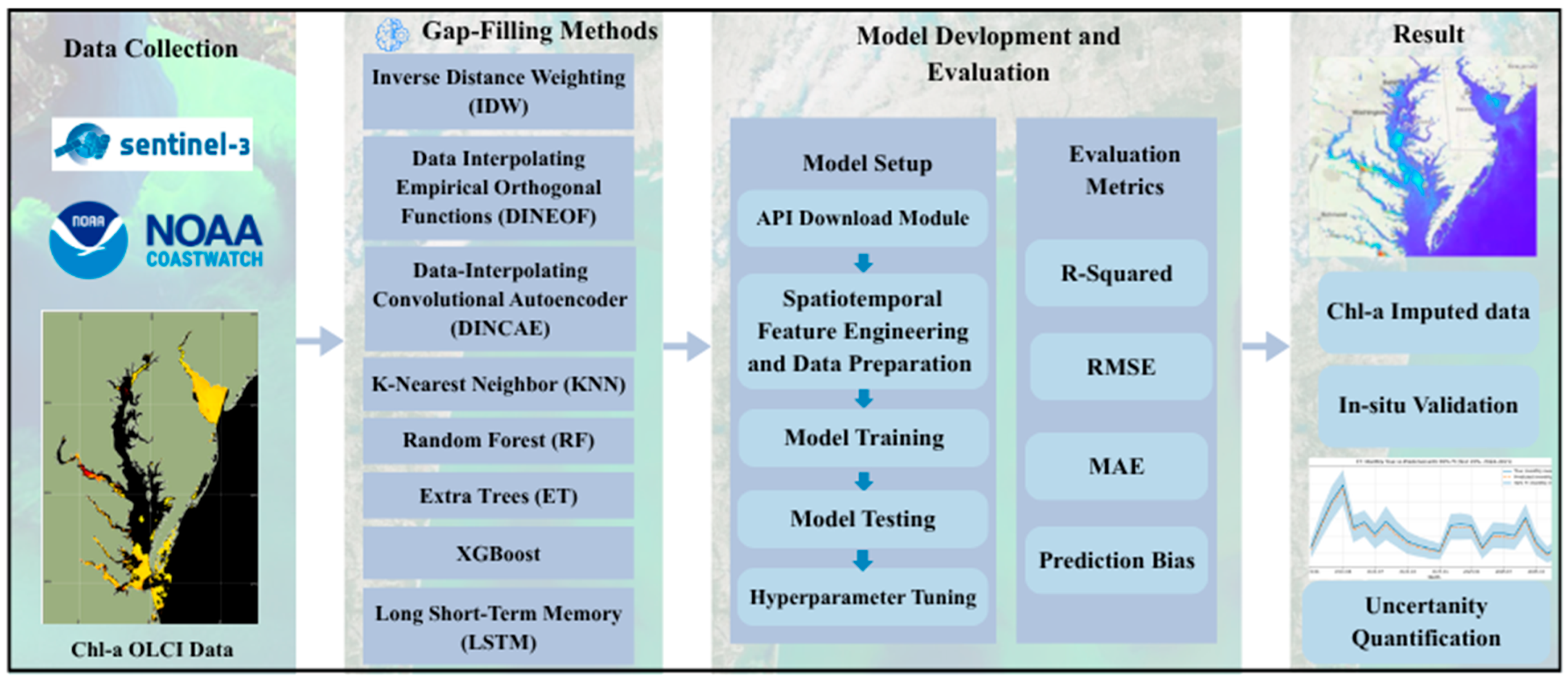
Figure 2 illustrates the methodological framework developed for Chl-a gap reconstruction in the Chesapeake Bay using spatial interpolation, supervised machine-learning, and deep-learning approaches. The workflow begins with the acquisition of daily Level-3 Chl-a products derived from the Sentinel-3 OLCI, accessed through the NOAA CoastWatch ERDDAP interface to ensure reproducible and standardized data retrieval [35]. To enable consistent data acquisition, structured API queries were used to request chlorophyll-a data over a fixed spatial bounding box corresponding to the Chesapeake Bay region and a defined temporal range spanning 2023–2025. Each query returns data in NetCDF format with consistent spatial resolution and metadata, enabling automated retrieval of daily observations. The downloaded daily datasets are systematically organized and stacked into a single multi-temporal NetCDF cube, where time is explicitly represented as a dimension. This stacking procedure preserves the spatiotemporal continuity of satellite observations and allows the dataset to be handled as a structured data cube rather than isolated images. The cube is subsequently clipped using a predefined Chesapeake Bay boundary shapefile to restrict analysis to the study region and eliminate irrelevant land pixels. This spatial filtering step reduces computational complexity and ensures that the modeling process focuses only on water bodies. This standardized and spatially constrained structure provides a consistent input foundation for subsequent preprocessing and modeling tasks.

Following data structuring, the workflow transitions to the data-driven modeling component of the framework [39]. The stacked and clipped data cube is transformed into a tabular dataset, where each valid pixel observation at a given time step is represented as an individual record. Predictor variables include spatial coordinates (latitude and longitude), temporal indicators such as day of year (encoded using sine and cosine transformations to capture seasonal patterns), and neighborhood-based statistical features that represent local spatial variability in chlorophyll concentration. These neighborhood features, including mean and standard deviation computed within a moving window, are derived using only available valid pixels to avoid introducing information from missing values. To further incorporate temporal dependencies, lag-based features (lag-1, lag-2, and lag-3) are constructed for each pixel location, enabling the models to capture short-term temporal continuity in Chl-a dynamics [40]. All predictor variables are standardized to ensure numerical stability and consistency across models. A set of gap-filling approaches—including spatial interpolation, EOF-based reconstruction, machine-learning, deep-learning, and convolutional autoencoder methods—is implemented within a unified experimental framework [41]. The spatial interpolation baseline consists of Inverse Distance Weighting (IDW), while Data Interpolating Empirical Orthogonal Functions (DINEOF) is used as the EOF-based reconstruction method. The machine-learning models include K-Nearest Neighbors (KNN), Random Forest (RF), Extra Trees (ET), and Extreme Gradient Boosting (XGBoost). In addition, a Long Short-Term Memory (LSTM) model is employed to explicitly capture temporal dependencies, while a Temporal Data Interpolating Convolutional Autoencoder (Temporal DINCAE) framework is implemented to learn spatial–temporal reconstruction patterns using convolutional encoder–decoder architecture. All machine-learning, deep-learning, and convolutional autoencoder models are trained using consistent input features and standardized preprocessing procedures to ensure a fair comparison. In contrast, the IDW baseline does not require model training and relies solely on spatial distance relationships between observed and missing pixels. This distinction ensures that the comparative evaluation reflects differences in modeling capability rather than inconsistencies in feature representation [16]. This design allows the framework to evaluate different learning methods for obtaining nonlinear spatial–temporal relationships in environmental data. By maintaining consistency in preprocessing and feature engineering, this design ensures that performance differences reflect algorithmic capability rather than preprocessing bias.

In the final stage, trained models are applied to predict chlorophyll concentrations at locations where observations are missing due to cloud cover or retrieval limitations. Machine-learning, deep-learning and convolutional autoencoder models generate predictions by learning spatial and temporal relationships from the data, whereas the IDW baseline reconstructs values using spatial distance-based interpolation and DINEOF reconstructs missing observations through EOF-based spatiotemporal decomposition. The predicted values are merged with the observed data to produce a spatially continuous chlorophyll dataset that maintains the original coordinate reference system and resolution. Model performance is quantitatively assessed using statistical evaluation metrics such as Root Mean Square Error (RMSE), Mean Absolute Error (MAE), prediction bias and the coefficient of determination (R²) to measure reconstruction accuracy and goodness of fit. These metrics provide objective evidence of model reliability and predictive strength. Overall, the architecture presented in Figure 2 provides a systematic, reproducible, and technically rigorous workflow that integrates satellite data acquisition, feature engineering, supervised learning, evaluation, and geospatial deployment into a unified modeling framework.

4.1. Inverse Distance Weighting (IDW)

Inverse Distance Weighting (IDW) was implemented as a spatial interpolation method to estimate missing Chl-a values based on nearby observations. The method assumes that spatial proximity corresponds to similarity, assigning greater weight to observations closer to the prediction location. Unlike machine-learning approaches, IDW does not require model training and relies directly on spatial relationships between known and unknown locations [42]. The prediction formulation is given in Equation (1).

$$\widehat{y}\left(x\right)={\displaystyle \frac{{\sum }_{i=1}^N\frac{y_i}{d_i^p}}{{\sum }_{i=1}^N\frac{1}{d_i^p}}}$$

(1)

$\widehat{y}\left(x\right)$ denotes the predicted chlorophyll-a value at location $x$, $yi$ denotes the observed value at the $i^{th}$ neighboring point, and $d_i$ is the spatial distance between the prediction location and the $i^{th}$ observation. The parameter $p$ controls the distance-decay rate, with larger values assigning greater weight to nearer neighbors.

IDW assumes smooth spatial variation and performs best in regions with strong spatial continuity. However, it does not account for temporal dynamics or nonlinear relationships, which may limit its effectiveness under large or irregular data gaps [16]. In this study, IDW is employed as a baseline method and evaluated under controlled artificial missingness scenarios to provide a benchmark for comparison with data-driven models.

4.2. Data Interpolating Empirical Orthogonal Functions (DINEOF)

Data Interpolating Empirical Orthogonal Functions (DINEOF) was applied as an EOF-based method for reconstructing missing chlorophyll-a (Chl-a) observations covered by cloud [43]. The method estimates missing values by identifying dominant spatial–temporal variability patterns within the dataset through iterative EOF decomposition [22]. The reconstruction is given in Equation (2).

$$X\approx U_k{S}_k{V}_k^T$$

(2)

where $X$ represents the missing Chl-a data matrix, $U_k$ and $V_k$ correspond to the spatial and temporal EOF components, and $S_k$ contains the singular values associated with the selected $k$ modes. Missing observations are iteratively reconstructed until the solution stabilizes.

DINEOF can effectively recover broad spatial–temporal structures under high missing-data rate, although localized variability and rapidly changing bloom patterns may become smoothed [44]. In this study, DINEOF was evaluated under controlled artificial missingness conditions as an EOF-based benchmark for comparison with supervised machine-learning, deep-learning, and convolutional autoencoder reconstruction models.

4.3. Supervised Machine Learning Models

The supervised modeling framework was designed to approximate the nonlinear relationship between spatial–temporal predictors and Chl-a concentration using historical satellite observations. Four regression algorithms were implemented to evaluate alternative learning mechanisms for gap reconstruction.

4.3.1. K-Nearest Neighbors (KNN)

K-Nearest Neighbors (KNN) regression was implemented as a non-parametric estimator operating within a multidimensional predictor space. For each prediction instance, Euclidean distances were computed across latitude, longitude, day-of-year, and neighborhood-based statistical features to identify the k most similar training samples. The predicted Chl-a value was calculated as a distance-weighted average of these neighbors [45]. Equation (3) represents the prediction formulation used in the KNN model.

$$\widehat{y}\left(x\right)={\displaystyle \frac{{\sum }_{i\in N_k\left(x\right)}{w}_i{y}_i}{{\sum }_{i\in N_k\left(x\right)}{w}_i}}$$

(3)

$N_k\left(x\right)$ represents the set of the $k$ nearest training samples for a given input location $x$. The term $y_i$ denotes the observed Chl-a value of the $i^{th}$ neighbor, while $w_i$ represents the weight assigned to that neighbor based on its distance from the prediction point. Neighbors that are closer in the predictor space receive higher weights and therefore contribute more strongly to the final prediction, while more distant observations have a smaller influence.

KNN assumes spatial smoothness and seasonal consistency under comparable environmental conditions. Because it does not impose an explicit functional relationship between predictors and the target variable, its predictive performance depends strongly on the density of training samples and the coverage of the feature space [46]. While this approach works well in environments exhibiting spatial coherence, such as the Chesapeake Bay, it remains sensitive to feature scaling and to the choice of the parameter $k$. In this study, the model was trained using spatial coordinates, temporal information, and neighborhood-based statistical predictors, and the value of $\mathrm{k}$ was experimentally adjusted to obtain stable prediction performance. KNN, therefore, serves as a baseline model for comparison with the ensemble-based approaches evaluated in this study.

4.3.2. Random Forest (RF)

Random Forest (RF) regression was employed as a bagging-based ensemble method to capture nonlinear interactions among predictors [47]. RF constructs multiple decision trees using bootstrap-resampled training subsets while randomly selecting a subset of predictors at each split. Each tree partitions the feature space independently, and predictions are averaged across trees to reduce variance. Equation (4) describes how the final prediction is obtained by averaging the outputs from all trees in the ensemble.

$$\widehat{y}\left(x\right)={\displaystyle \frac{1}{T}}{\sum }_{t=1}^T{f}_t\left(x\right)$$

(4)

$T$ represents the total number of decision trees in the ensemble, and $f_t(x)$ denotes the prediction generated by the $t^{th}$ tree for input sample $x.$ The final predicted Chl-a value is obtained by averaging the outputs from all trees, which reduces prediction variance and improves model stability.

This ensemble aggregation allows RF to model complex, hierarchical relationships without assuming linearity [48]. In coastal systems, where chlorophyll dynamics are influenced by localized bloom intensification, seasonal transitions, and spatial gradients, RF effectively captures structured variability. The random selection of predictors during tree construction reduces correlation among trees and helps mitigate overfitting [49]. In this study, the RF model was trained using the same spatial and temporal predictor variables used across all models, and key parameters such as the number of trees and maximum tree depth were experimentally adjusted to achieve stable prediction performance [50].

4.3.3. Extra Trees (Extremely Randomized Trees)

Extra Trees extends the RF framework by introducing additional stochasticity during split selection. Instead of optimizing split thresholds based on impurity reduction, candidate thresholds are selected randomly. Trees are typically constructed using the full training dataset, while randomness in feature selection and split thresholds increases ensemble diversity [51]. Equation (5) shows how the final prediction is obtained by averaging the outputs from multiple randomized trees.

$$\widehat{y}\left(x\right)={\displaystyle \frac{1}{T}}{\sum }_{t=1}^T{f}_t^{random}\left(x\right)$$

(5)

$T$ represents the total number of trees in the ensemble, and $f_t^{random}(x)$ denotes the prediction produced by the $t^{th}$ tree built using randomly selected split thresholds. The final predicted value is obtained by averaging the predictions from all trees, which helps reduce variance and improve model stability.

This enhanced randomization reduces tree correlation and can lower model variance, improving generalization stability. For satellite-derived environmental data—often characterized by noise and spatial discontinuities—such ensemble diversity is advantageous [52]. Extra Trees demonstrated strong capability in representing nonlinear gradients and seasonal variability while maintaining computational efficiency, making it particularly suitable for large-scale gap-filling tasks [15].

4.3.4. Extreme Gradient Boosting (XGBoost)

Extreme Gradient Boosting (XGBoost) was implemented as a boosting-based regression framework to iteratively minimize prediction error. Unlike bagging methods, which build trees independently, XGBoost constructs trees sequentially, with each new tree trained to correct residual errors from the existing ensemble. This gradient-based optimization allows incremental refinement of predictions [53]. Equation (6) describes the prediction method used in the XGBoost model.

$$\widehat{y_i}={\sum }_{k=1}^K{f}_k\left(x_i\right)$$

(6)

$f_k$ represents the prediction produced by the $k^{th}$ regression tree, and $K$ denotes the total number of trees in the boosting sequence. The final predicted value is obtained by summing the contributions of all trees, where each new tree focuses on reducing the residual errors from previous trees.

Regularization terms, learning-rate control, and tree-depth constraints were incorporated to balance model complexity and generalization. The boosting mechanism places greater emphasis on difficult-to-predict instances, such as abrupt seasonal transitions or localized bloom intensification events. By sequentially minimizing residuals, XGBoost captures subtle nonlinear dependencies among spatial coordinates, seasonal indicators, and contextual features. XGBoost provides an adaptive learning approach that improves bias reduction and predictive accuracy for chlorophyll gap reconstruction in cloud-affected satellite imagery [54].

4.4. Long Short-Term Memory (LSTM)

Long Short-Term Memory (LSTM) networks were implemented as a deep-learning approach to model temporal dependencies in Chl-a dynamics. Unlike traditional machine-learning models that treat observations independently, LSTM processes sequential data and captures temporal dependencies across multiple time steps. This capability is particularly important for environmental time series, where chlorophyll concentrations exhibit persistence, seasonal cycles, and short-term variability [55]. The prediction formulation is given in Equation (7).

$$\widehat{y_t}=W_h\cdot \mathrm{LSTM}\left(x_t,h_{t-1},c_{t-1}\right)+b$$

(7)

$x_t$ denotes the input feature vector at time step t, while $h_{t-1}$ and $c_{t-1}$ represent the hidden and cell states from the previous time step, respectively. The LSTM captures temporal dependencies by modeling the influence of past observations on current chlorophyll-a values. The predicted output $\widehat{y_t}$ is obtained by applying a linear transformation with weights $W_h$ and bias $b$ to the learned temporal representation.

In this study, input sequences were constructed using fixed-length temporal windows for each spatial pixel, incorporating spatial, seasonal, and lag-based features at each time step. This formulation enables the model to jointly capture spatial context and temporal evolution [55]. Although LSTM effectively models temporal continuity and dynamic variability, its performance depends on the availability of sufficiently long sequential data and appropriate parameter tuning [56].

4.5. Temporal Data Interpolating Convolutional Autoencoder (Temporal DINCAE)

The Temporal Data Interpolating Convolutional Autoencoder (Temporal DINCAE) was implemented as a convolutional autoencoder-based reconstruction model for estimating missing Chl-a observations from incomplete satellite imagery. The model combines convolutional encoder–decoder architecture with temporal and spatial feature representation to learn nonlinear reconstruction patterns directly from the data [57]. The prediction formulation is given in Equation (8).

$$\widehat{Y}=f\theta \left(X\right)$$

(8)

where $X$ represents the multi-channel input feature tensor, $f\theta$ denotes the convolutional autoencoder parameterized by learnable weights $\theta$, $\widehat{Y}$ is the reconstructed Chl-a output. The model was trained using masked reconstruction loss to estimate missing observations while preserving spatial–temporal continuity.

Temporal DINCAE enables the reconstruction of complex nonlinear Chl-a variability by integrating spatial structure, temporal dependencies, and seasonal dynamics within a unified framework [58]. In this study, the model was evaluated as a convolutional autoencoder-based approach for comparison with EOF-based, supervised machine-learning, and deep-learning reconstruction methods.

4.6. Spatiotemporal Feature Engineering and Data Preparation

Prior to model development, the Chl-a dataset was transformed from a multi-dimensional raster format into a tabular structure compatible with regression-based modeling approach. Each valid pixel–time pair was treated as an independent observation, enabling the modeling of spatial–temporal relationships. Geographic coordinates (latitude and longitude) were retained as continuous predictors to preserve large-scale spatial gradients across the study domain. Seasonal dynamics were encoded using day-of-year (DOY), which was further encoded using sine and cosine transformations to represent cyclical temporal patterns. These features enable the models to capture recurring intra-annual bloom dynamics while avoiding artificial discontinuities at the start and end of the year. Together, the spatial and temporal predictors represent the primary drivers of chlorophyll variability in estuarine systems, including spatial gradients associated with riverine inputs, seasonal phytoplankton cycles, and local spatial autocorrelation [59].

To incorporate short-range spatial context, neighborhood-derived statistics were calculated for each pixel, including local mean and standard deviation values from adjacent grid cells using a fixed 3 × 3 moving window centered on the target pixel. These contextual features enhance the representation of spatial continuity and reduce sensitivity to isolated noise [60]. To ensure reproducibility and prevent data leakage, neighborhood statistics were computed exclusively from valid (non-missing) chlorophyll-a values within the window, without any prior imputation or interpolation. Pixels with missing neighboring values were excluded from the computation, and observations with insufficient valid data were removed during preprocessing. Observations containing undefined predictor variables were removed to prevent numerical instability during training. Feature matrices were constructed with consistent column ordering, and redundant or duplicated attributes were eliminated to maintain structural integrity. For the Temporal DINCAE framework, the engineered variables were additionally organized into an 18-channel spatial–temporal input representation consisting of temporal lag variables, observation masks, current chlorophyll-a observations, spatial coordinates, seasonal sine and cosine features, neighborhood-based statistics, and temporal trend variables. This multi-channel formulation enabled the model to jointly learn spatial, temporal, and seasonal reconstruction patterns from incomplete observations.

To improve numerical stability and regression performance, the response variable was transformed using log(1 + Chl-a), reducing skewness associated with episodic bloom peaks and stabilizing variance across concentration ranges. This transformation facilitates smoother decision boundaries for tree-based, distance-based, deep-learning, and convolutional autoencoder models. Predictor variables were inspected to ensure consistent units and appropriate scaling, particularly for distance-sensitive algorithms such as KNN. Missing Chl-a values were excluded from the training dataset to avoid bias in parameter estimation. The DINEOF framework used iterative EOF decomposition of dominant spatial–temporal variability patterns for reconstructing missing observations. Data from 2023–2024 were used for model training, while data from 2025 were reserved for testing. This temporal split avoids spatiotemporal leakage and enables a more realistic assessment of model performance on unseen future observations. Feature and target arrays were formatted for compatibility with scikit-learn and gradient boosting implementations. All preprocessing steps were applied uniformly across KNN, Random Forest, Extra Trees, XGBoost, LSTM, and Temporal DINCAE to ensure methodological consistency. This structured preprocessing pipeline establishes a stable and statistically rigorous foundation for EOF-based, supervised machine-learning, deep-learning, and convolutional autoencoder reconstruction of satellite-derived Chl-a data.

4.7. Model Training

Model training was conducted within a temporally consistent framework, with Chl-a observations from 2023–2024 used for training and data from 2025 reserved as an independent test set. This temporal separation ensures evaluation on unseen future observations, thereby preventing spatiotemporal leakage and enabling a more realistic assessment of model generalization. The response variable was modeled using a log-transformed formulation, log(1 + Chl-a), to stabilize variance and mitigate the influence of extreme bloom events. The DINEOF framework reconstructed missing observations using iterative EOF decomposition of dominant spatial–temporal variability patterns through repeated singular-value decomposition until convergence was achieved.

Machine-learning models, including K-Nearest Neighbors (KNN), Random Forest (RF), Extra Trees (ET), and XGBoost, were implemented within a unified experimental framework. For the K-Nearest Neighbors model, the optimal number of neighbors was selected to balance local sensitivity and smoothing in feature space, with distance-based weighting applied to emphasize closer observations. Random Forest and Extra Trees were trained as ensemble tree-based models to capture nonlinear interactions among predictors. Hyperparameters such as the number of estimators and maximum tree depth were tuned to provide adequate model capacity while controlling variance. Bootstrap sampling and randomized feature selection were applied to enhance generalization stability. XGBoost was trained using gradient-based boosting to sequentially minimize residual errors. Learning rate, tree depth, subsampling, and regularization parameters were configured to control model complexity and ensure stable convergence. Fixed random seeds were applied across ensemble-based methods to ensure reproducibility. Computational implementation leveraged optimized machine-learning libraries to efficiently handle the large spatiotemporal dataset.

In parallel, a Long Short-Term Memory (LSTM) network was developed to capture temporal dependencies in Chl-a dynamics. Sequential input data were constructed for each spatial pixel using fixed-length temporal windows, enabling the model to learn temporal evolution patterns across multiple time steps. To maintain sequence continuity, missing chlorophyll-a values were first estimated using an XGBoost-based gap-filling approach, thereby ensuring complete input sequences. Unlike traditional models that treat observations independently, LSTM processes ordered data and leverages historical information through its internal memory structure. Spatial, seasonal, and lag-based features were incorporated at each time step to jointly represent spatial context and temporal variability. This design enables the model to capture dynamic processes such as seasonal transitions and short-term fluctuations. By relying exclusively on past observations, the sequence formulation avoids temporal leakage. However, model performance depends on the availability of sufficient sequential data and appropriate parameter tuning for stable generalization.

Feature ordering and dimensional consistency were strictly maintained throughout training to avoid structural mismatches during deployment. In addition, the Temporal DINCAE framework was implemented as a convolutional autoencoder-based reconstruction model using multi-channel spatial–temporal input tensors. The model incorporated spatial coordinates, seasonal indicators, neighborhood-based statistics, temporal lag features, and observation masks within a convolutional encoder–decoder architecture to learn nonlinear reconstruction patterns from incomplete chlorophyll-a observations. Iterative reconstruction was applied during inference to progressively estimate missing regions while preserving spatial–temporal continuity. The IDW method, which does not require model training, was applied independently during the reconstruction stage by identifying neighboring valid pixels, computing distance-based weights, and estimating missing values through weighted spatial averaging. Model fitting for machine learning and deep learning approaches was monitored to ensure numerical stability and prevent data leakage from missing-value placeholders. Finalized model objects were serialized and stored for subsequent gap reconstruction. This structured training protocol ensures that the models effectively capture nonlinear spatial–temporal relationships while maintaining computational robustness and reproducibility.

4.8. Model Testing

Model performance was assessed using the temporally independent test dataset from 2025, which was strictly excluded from model training and hyperparameter tuning. This separation ensured an unbiased evaluation of predictive generalization. The testing samples retained the identical predictor structure used during training, including latitude, longitude, day-of-year, and neighborhood-based contextual statistics. All preprocessing steps, including feature ordering and transformation, were applied consistently to prevent structural discrepancies between training and testing phases. Predictions were generated in the log-transformed space and subsequently back-transformed to the original Chl-a concentration scale using the inverse log(1 + x) transformation. Only observations with valid measured Chl-a values were included in the evaluation to allow direct comparison between predicted and observed concentrations. Spatial and temporal alignment was preserved throughout the testing process to maintain consistency with the original data structure. For the IDW baseline, performance was evaluated separately on the same test dataset to ensure a consistent reference for comparison with data-driven models.

4.9. Hyperparameter Tuning

Hyperparameter tuning was performed to optimize model performance and improve generalization for Chl-a gap reconstruction. A temporally separated tuning strategy was adopted to eliminate spatiotemporal leakage. Data from 2023 were used for model fitting, data from 2024 for validation and parameter selection, and data from 2025 as an independent test set. After selecting the optimal parameters, the models were retrained using the combined 2023–2024 dataset and evaluated on the 2025 test set. A structured search strategy (

Table 1. Parameter optimization ranges and search strategy for supervised learning models.

Model	Hyperparameter	Search Space	Search Method
KNN	n_neighbors	3–15	Grid Search
	weights	Uniform, distance	Choice
	p (distance metric)	1, 2	Choice
Random Forest	n_estimators	300–800	Random Search
	Max_depth	None, 10–40	Choice
	min_samples_split	2–10	Grid Search
	min_samples_leaf	1–5	Grid Search
	max_features	sqrt, log2	Choice
Extra Trees	n_estimators	400–1000	Random Search
	max_depth	None, 10–40	Choice
	min_samples_split	2–8	Grid Search
	min_samples_leaf	1–4	Grid Search
	max_features	Sqrt, log2	Choice
XGBoost	n_estimators	300–800	Random Search
	learning_rate	0.01–0.1	Log-uniform
	max_depth	3–10	Grid Search
	subsample	0.6–1.0	Random Search

) was implemented to systematically explore the parameter space for each model, and the final selected hyperparameters are summarized in

Table 2. Final selected hyperparameters.

Model	Hyperparameter
IDW	Power = 2, neighbors = 8
DINEOF	EOF modes = 10, max iterations = 30
KNN	k = 5, weights = distance, p = 2
RF	n_estimators = 300, max_depth = 20
ET	n_estimators = 300, max_depth = 20
XGBoost	n_estimators = 500, learning_rate = 0.05, max_depth = 6, subsample = 0.8
LSTM	Sequence length = 24, hidden size = 384, layers = 2, dropout = 0.25, learning rate = 0.0003
Temporal DINCAE	Input channels = 18, base filters = 64, dropout = 0.10, batch size = 16, learning rate = 0.0001

. For the DINEOF framework, tuning focused on the number of EOF modes and convergence iterations used during iterative reconstruction. The selected configuration utilized 10 EOF modes and iterative convergence criteria that provided stable reconstruction performance under controlled missingness conditions. For the KNN model, the number of neighbors $k$ was optimized, as it determines how many nearby observations are used for prediction. The influence of each neighbor, represented through the weighting term $w_i$, was controlled by tuning the distance metric parameter $p$ and the weighting scheme, which affects how strongly closer samples contribute to the final estimate. The final configuration selected was k = 5, with distance-based weighting and p = 2, providing a balance between local sensitivity and smoothing.

For the ensemble-based models, tuning focused on parameters that control the structure and complexity of the decision trees. In Random Forest and Extra Trees, the number of trees $T$ was optimized, as it determines how many individual models are combined in the final prediction. Additional parameters such as maximum tree depth, minimum samples required for splitting, and minimum samples per leaf were tuned to regulate how each tree function $f_t(x)$ partitions the feature space. These parameters influence the ability of the models to capture nonlinear spatial and seasonal patterns while maintaining stability and avoiding overfitting. For the XGBoost model, tuning focused on parameters controlling the sequential boosting process. The number of boosting iterations $K$ was optimized to determine how many trees contribute to the final prediction. Parameters such as maximum tree depth and subsampling ratio were adjusted to control model complexity and improve robustness. The learning rate η, although not explicitly shown in the model equation, was also tuned to regulate the contribution of each tree during error correction. The final configuration consisted of 500 estimators, a learning rate of 0.05, a maximum depth of 6, and a subsampling ratio of 0.8, resulting in strong predictive performance and stable convergence.

For the LSTM model, hyperparameter tuning focused on parameters governing temporal representation and training stability. The sequence length, hidden layer size, number of layers, dropout rate, optimizer, and learning rate were systematically adjusted to effectively capture temporal dependencies. The final configuration—sequence length of 24, hidden size of 384, two LSTM layers, dropout rate of 0.25, AdamW optimizer, and learning rate of 0.0003—resulted in stable training and improved generalization. For the Temporal DINCAE framework, hyperparameter tuning focused on convolutional architecture depth, dropout rate, batch size, masking fraction, and learning rate. The final configuration utilized an 18-channel input representation, a three-level convolutional encoder–decoder architecture, base filter size of 64, dropout rate of 0.10, batch size of 16, and learning rate of 0.0001, resulting in stable convergence and strong reconstruction performance.

Model selection was primarily guided by the R² evaluated on the validation subset, with RMSE used as a complementary metric to monitor absolute error magnitude. Overfitting was assessed by comparing training and validation performance to avoid overly complex configurations. The final tuned models demonstrated consistent validation performance and stable generalization behavior. This systematic optimization process ensured that reported performance gains reflect genuine improvements in model structure rather than arbitrary parameter choices, thereby enhancing the reliability and robustness of Chl-a reconstruction.

4.10. Model Evaluation

Model performance was evaluated using four standard regression metrics to ensure a clear and consistent assessment of prediction accuracy and error behavior. These metrics include the R², RMSE, MAE, and prediction bias. RMSE quantifies the overall magnitude of prediction errors and is more sensitive to larger deviations, while MAE provides a complementary measure of the average absolute differences between predicted and observed values. R² evaluates the explanatory strength of the model by measuring the proportion of variance captured in unseen data. Prediction bias was also computed to identify any systematic tendency to overestimate or underestimate Chl-a concentrations. All metrics were computed on the independent testing dataset to ensure that the evaluation reflects true model performance on unseen data. These metrics are applied to the predicted values $\widehat{y_i}$ obtained from the model formulations described in Equations (9) and (10).

The R², defined in Equation (9), measures how well the predicted values match the observed Chl-a concentrations [61]. It represents the proportion of variance explained by the model, where a higher value indicates better predictive performance.

$$R^2=1-{\displaystyle \frac{{\sum }_{i=1}^n{\left(y_i-\widehat{y_i}\right)}^2}{{\sum }_{i=1}^n{\left(y_i-\overline{y}\right)}^2}}$$

(9)

In this equation, $y_i$ represents the observed Chl-a value, $\widehat{{\mathrm{y}}_{\mathrm{i}}}$ represents the predicted value obtained from the model, $\overline{\mathrm{y}}$ is the mean of observed values, and $n$ is the total number of samples. These variables are consistently used across all evaluation metrics.

RMSE, shown in Equation (10), measures the overall magnitude of prediction errors and gives greater weight to larger errors, making it useful for identifying significant deviations [61].

$$RMSE=\sqrt{{\displaystyle \frac{1}{n}}{\sum }_{i=1}^n{\left(y_i-\widehat{y_i}\right)}^2}$$

(10)

MAE, defined in Equation (11), calculates the average absolute difference between predicted and observed values, providing a simple and interpretable measure of typical prediction error [50].

$$MAE={\displaystyle \frac{1}{n}}{\sum }_{i=1}^n\left|y_i-\widehat{y_i}\right|$$

(11)

Prediction bias, given in Equation (12), evaluates whether the model consistently overestimates or underestimates Chl-a values [62]. A value close to zero indicates that the model does not exhibit systematic deviation.

$$Bias={\displaystyle \frac{1}{n}}{\sum }_{i=1}^n\left(\widehat{y_i}-y_i\right)$$

(12)

Collectively, these metrics provide a comprehensive evaluation framework by capturing explained variance (R²), overall error magnitude (RMSE), average deviation (MAE), and systematic bias (Bias), ensuring a reliable and consistent comparison of all models used in this study.

5. Results

5.1. Comparative Model Performance

The predictive performance of the evaluated models was assessed using a temporally independent test dataset from 2025, ensuring an unbiased evaluation of model generalization. While the IDW baseline provides simple distance-based interpolation, it lacks the capacity to capture complex spatiotemporal variability under high missing-data conditions. Similarly, the EOF-based DINEOF framework effectively reconstructs dominant large-scale spatial–temporal patterns but tends to smooth localized variability and rapidly changing bloom structures. The results show a clear relationship between model structure and predictive performance. The distance-based KNN approach provides stable local interpolation but shows limited capability in capturing broader nonlinear spatial–seasonal interactions. Random Forest improves performance by modeling nonlinear relationships through ensemble averaging, enhancing robustness under heterogeneous chlorophyll conditions. Extra Trees further increases ensemble diversity by introducing randomized split thresholds, which improves generalization stability by reducing tree correlation. In contrast, the boosting-based XGBoost framework enables sequential learning of residuals, allowing more effective representation of complex environmental patterns. The LSTM model further extends this capability by explicitly incorporating temporal dependencies, enabling improved representation of seasonal evolution and short-term chlorophyll variability. The convolutional autoencoder-based Temporal DINCAE framework additionally captures nonlinear spatial–temporal reconstruction patterns through multi-channel feature integration, enabling effective reconstruction of missing chlorophyll-a observations under extensive cloud-cover conditions.

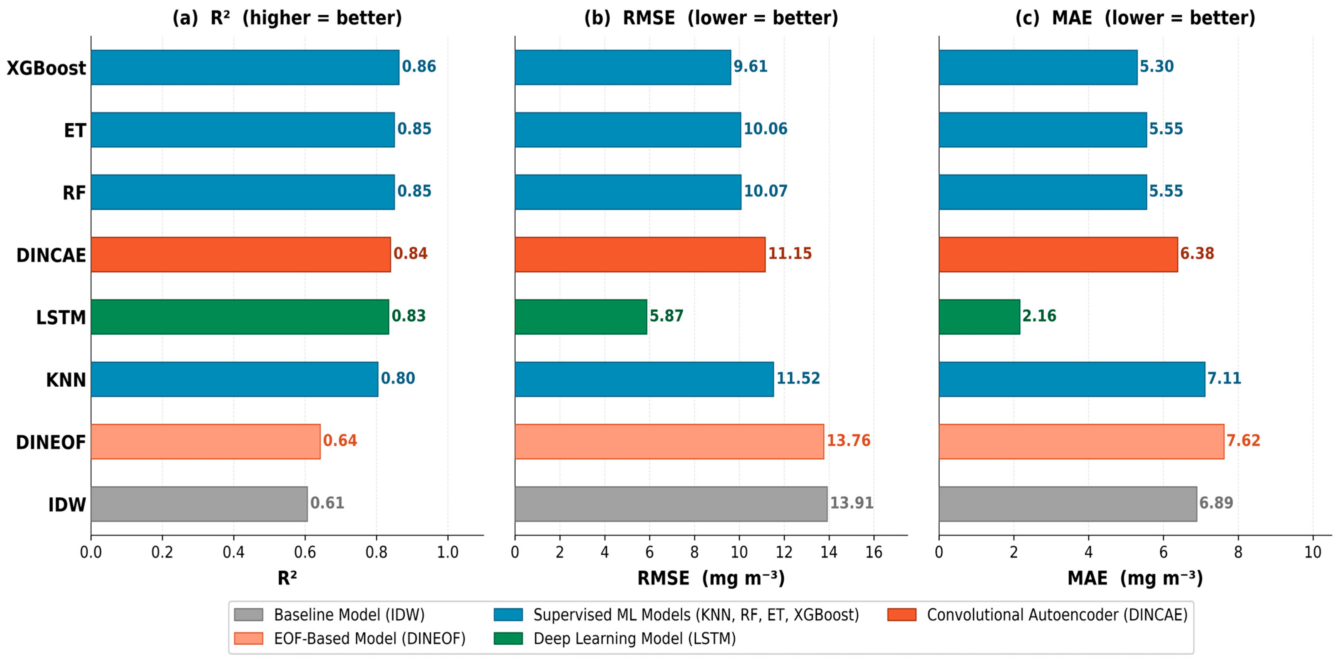
To quantify these differences, model performance was evaluated using RMSE, MAE, and R² on the temporally independent 2025 test dataset. XGBoost achieved the highest predictive accuracy, with R² = 0.86, RMSE = 9.61 mg m⁻³, and MAE = 5.30 mg m⁻³, indicating strong explanatory power and low prediction error. Extra Trees and Random Forest showed comparable performance, with Extra Trees yielding R² = 0.85, RMSE = 10.06 mg m⁻³, and MAE = 5.55 mg m⁻³, and Random Forest producing R² = 0.85, RMSE = 10.07 mg m⁻³, and MAE = 5.55 mg m⁻³. KNN demonstrated relatively lower performance, with R² = 0.80, RMSE = 11.52 mg m⁻³, and MAE = 7.11 mg m⁻³, reflecting higher prediction errors and reduced ability to capture complex variability. The LSTM model achieved the lowest prediction errors, with RMSE = 5.87 mg m⁻³, MAE = 2.16 mg m⁻³, and R² = 0.83, demonstrating a strong ability to capture temporal dynamics while maintaining competitive explanatory performance. The Temporal DINCAE model achieved competitive reconstruction performance, with R² = 0.84, RMSE = 11.15 mg m⁻³, and MAE = 6.38 mg m⁻³, demonstrating the capability of convolutional autoencoder-based reconstruction for capturing nonlinear spatial–temporal variability. The EOF-based DINEOF framework produced moderate reconstruction performance, with R² = 0.64, RMSE = 13.76 mg m⁻³, and MAE = 7.62 mg m⁻³, indicating its effectiveness in reconstructing dominant large-scale spatial–temporal structures despite high missing-data conditions. In contrast, the IDW baseline exhibited the weakest performance (R² = 0.61, RMSE = 13.91 mg m⁻³, MAE = 6.89 mg m⁻³), underscoring the limitations of purely distance-based interpolation in representing complex spatiotemporal variability.

These quantitative results are summarized in Figure 3, which compares model performance across RMSE, MAE, and R². While all models capture the primary variability in Chl-a concentrations, clear differences in predictive accuracy are evident. The IDW baseline exhibits the highest error values, reflecting its limited ability to represent complex spatiotemporal variability. The EOF-based DINEOF framework improves reconstruction capability relative to IDW by capturing dominant spatial–temporal patterns, although its performance remains lower than the data-driven reconstruction models. Ensemble-based approaches provide improved accuracy and stability, with XGBoost consistently achieving the best overall performance. Extra Trees and Random Forest also perform strongly, yielding comparable results. In contrast, the higher error values observed for KNN suggest sensitivity to local data distribution and reduced generalization capability. The LSTM model achieves the lowest RMSE and MAE values, underscoring its effectiveness in capturing temporal dynamics; however, its R² remains slightly lower than that of XGBoost, indicating a modest reduction in variance explanation. The Temporal DINCAE framework achieved competitive performance, with reconstruction accuracy higher than KNN, DINEOF, and IDW, while remaining slightly lower than the ensemble-based models.

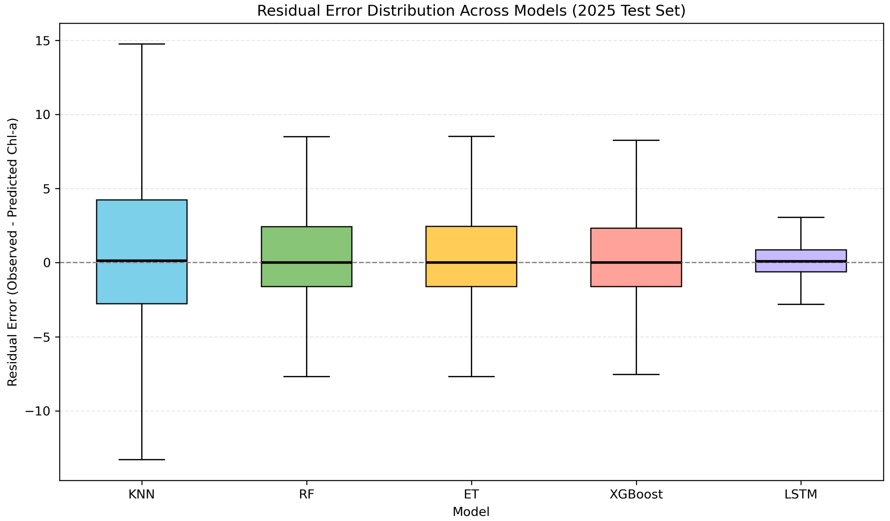
To further understand model behavior in detail, the distribution of residual prediction errors was examined. This analysis provides a clearer view of prediction consistency and systematic deviation across varying Chl-a conditions. As shown in Figure 4, the residuals for all models are centered close to zero, indicating that there is no strong systematic overestimation or underestimation in the predictions. However, a slight tendency toward underestimation is observed across all models, as indicated by the negative bias values. KNN shows a bias of −1.53, Random Forest −1.32, Extra Trees −1.32, and XGBoost −1.14, indicating that predictions are, on average, slightly lower than the observed concentrations. In contrast, the LSTM model exhibits a substantially lower bias of −0.26, suggesting improved calibration and reduced systematic error relative to the other approaches. Despite this, the bias remains small in magnitude, confirming that all models maintain stable and well-calibrated predictions.

Differences in residual spread provide further insight into model stability and consistency. XGBoost exhibits a narrower distribution of residuals, indicating more consistent performance across the dataset. Random Forest and Extra Trees show moderate dispersion, reflecting balanced behavior with reduced variance due to ensemble averaging. In contrast, KNN displays a wider spread of residuals, suggesting greater variability in prediction error and reduced stability, particularly under heterogeneous environmental conditions. The LSTM model exhibits the most compact residual distribution, indicating improved prediction consistency and reduced error variability, attributable to its ability to capture temporal dependencies.

5.2. Time Series and Spatial Distribution

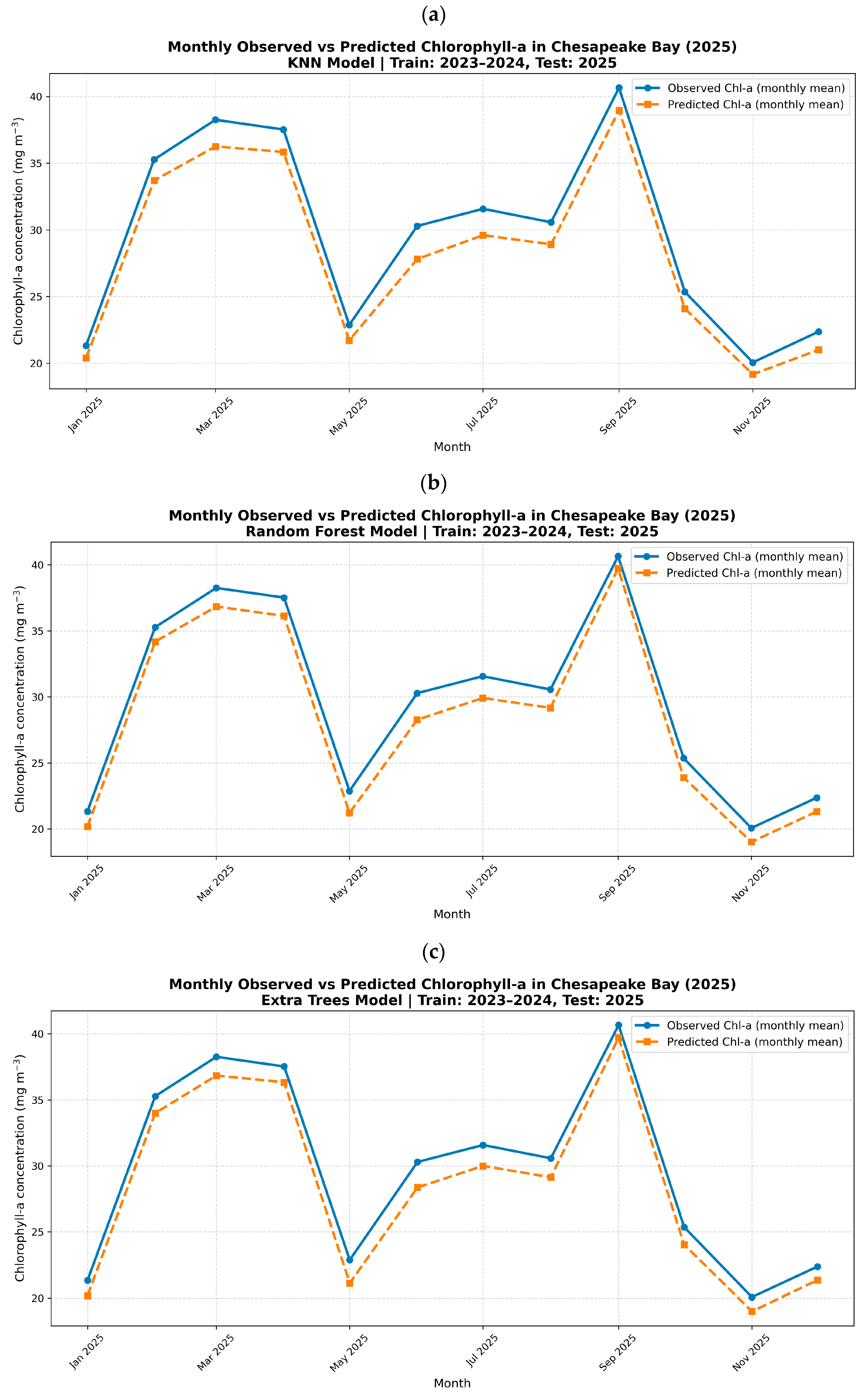
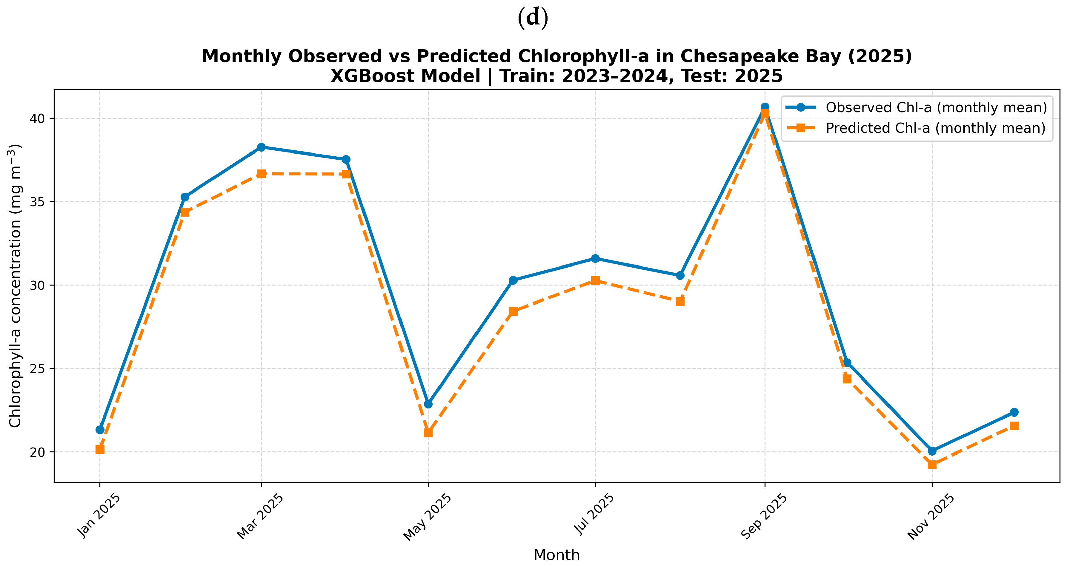
The time series behavior of Chl-a concentrations was analyzed using monthly averages for the 2025 test period. The monthly comparison (Figure 5) demonstrates that all models successfully reproduce the progression of Chl-a, including the rapid increase from winter baseline levels (~20 mg m⁻³) to a peak during late summer (~40 mg m⁻³), followed by a sharp decline toward the end of the year. Predicted monthly means closely track observed values across all models, indicating that the dominant bloom cycle relevant for HAB monitoring is preserved after gap reconstruction. Among the models, XGBoost and Extra Trees show the closest agreement with observed values across most months, with minimal deviations during both peak and transition periods. In contrast, KNN exhibits larger deviations, particularly during periods of rapid change, highlighting its limited capacity to capture broader temporal variability. Despite these differences, all models preserve the timing of key seasonal transitions, including the onset, peak, and decline phases of chlorophyll concentration. Overall, the results demonstrate that the gap-filling framework effectively preserves temporal dynamics while improving data continuity. The ability of the models to accurately reproduce seasonal variability indicates that the reconstructed datasets retain essential environmental signals necessary for reliable monitoring of chlorophyll dynamics and HAB-related processes in the Chesapeake Bay.

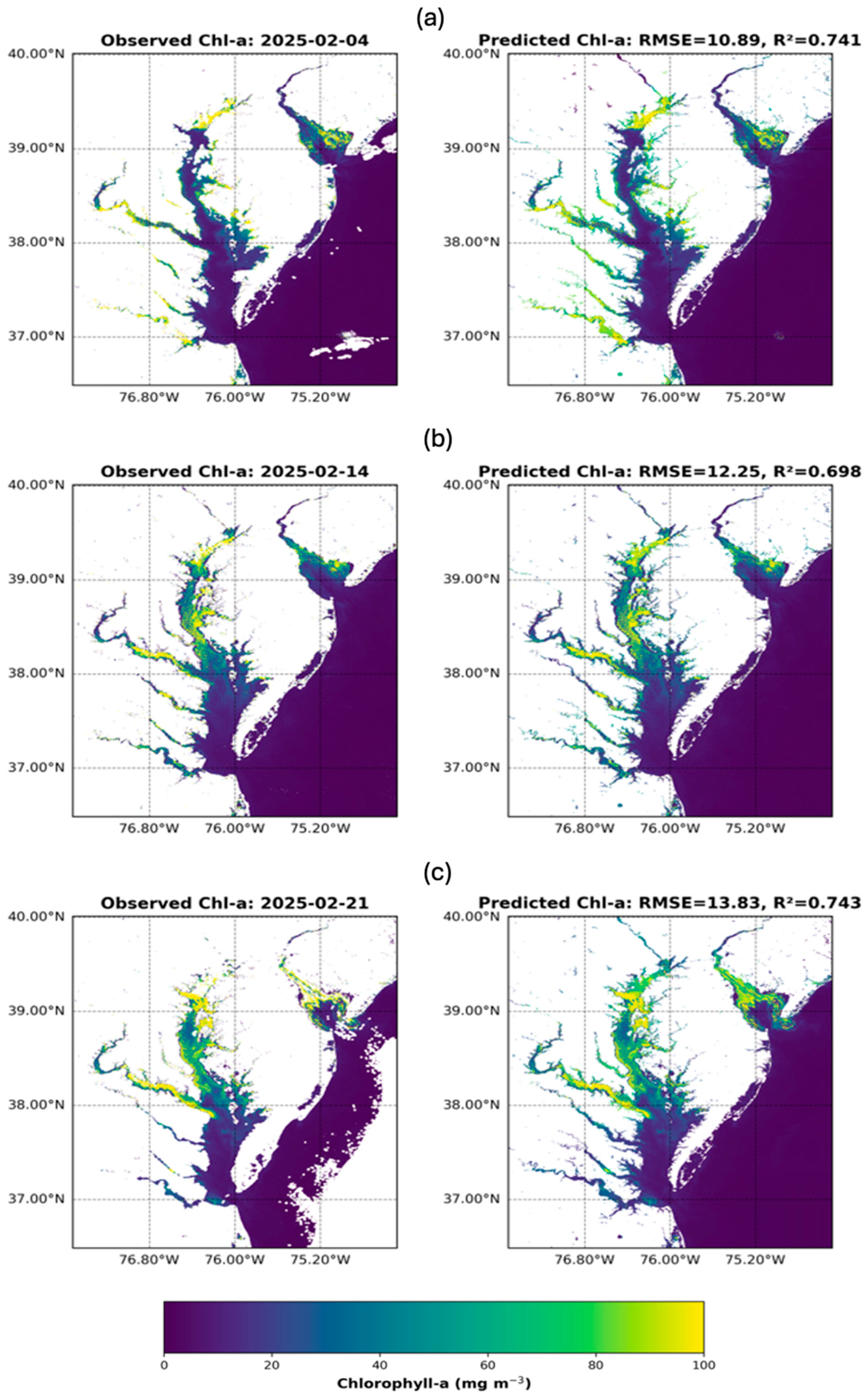
To evaluate spatial consistency, the reconstructed Chl-a distributions were examined for selected cloud-affected days using the XGBoost model. As shown in Figure 6, the observed Chl-a (left) and XGBoost-based reconstructed Chl-a (right) are presented for three representative dates: 4 February 2025, 14 February 2025, and 21 February 2025, with corresponding missing data rates of 11.97%, 6.73%, and 39.62%, respectively. The reconstructed maps demonstrate that the XGBoost model effectively fills missing regions while maintaining realistic spatial patterns of chlorophyll concentration. The distribution of high- and low-concentration areas remains consistent with observed conditions, indicating that important spatial features are well retained after reconstruction. Notably, even for the higher missing rate case (39.62%), the model is able to reconstruct spatial patterns with reasonable accuracy, indicating robustness under data-sparse conditions. A slight underestimation is observed in areas of high chlorophyll concentration, particularly in the upper and mid-Bay regions shown in Figure 6a,c, where peak values appear slightly reduced in the reconstructed maps compared to the observed data. This effect is more noticeable on 21 February 2025 (Figure 6c), which also corresponds to the highest missing data rate, and is likely due to ensemble averaging and the variance-stabilizing transformation applied during training. These results support the reliability of ensemble-based methods for operational HAB monitoring in cloud-affected coastal environments.

5.3. Evaluation Under Controlled Missing Data Conditions

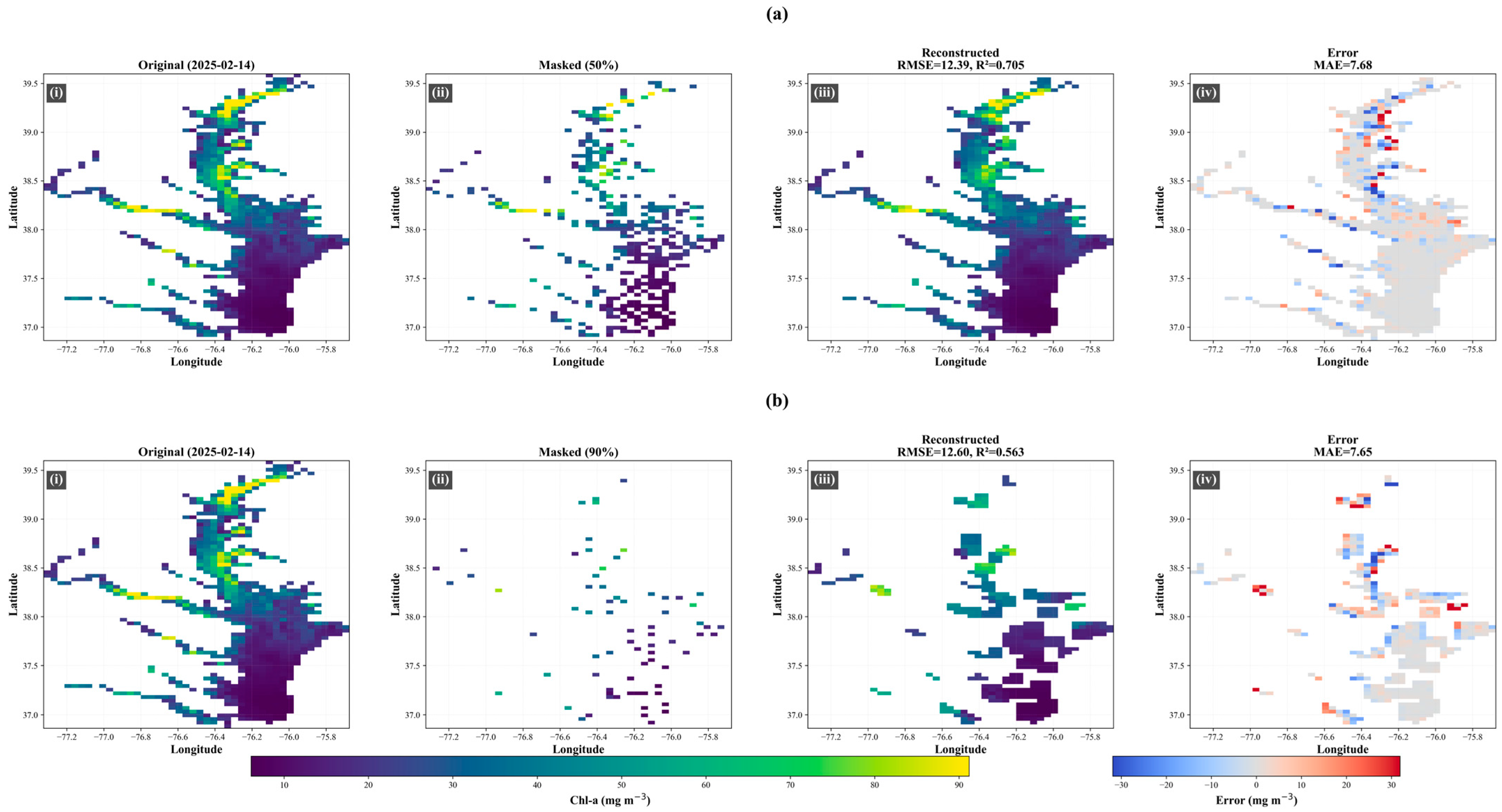
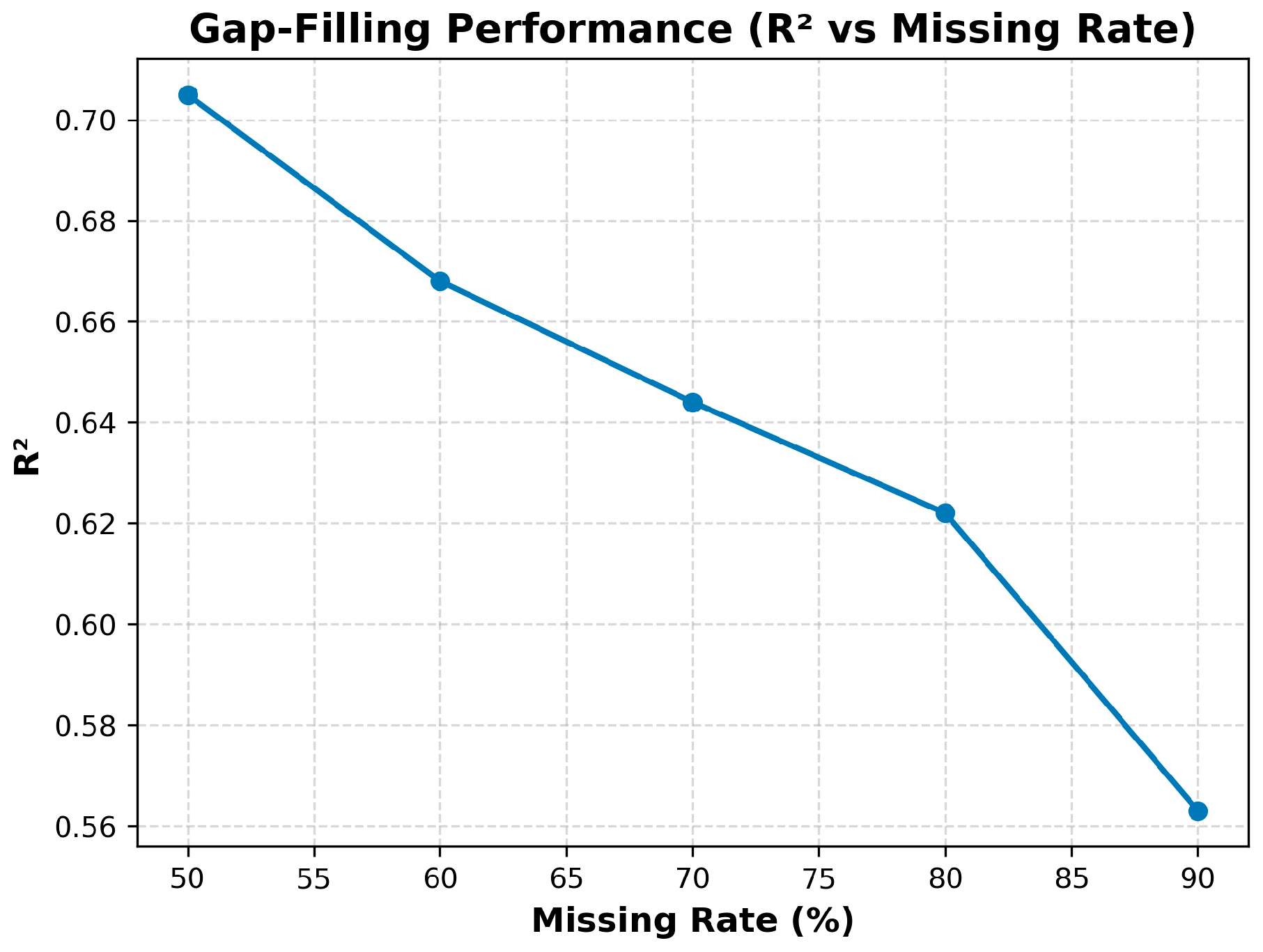
To evaluate whether model performance reflects realistic gap-filling conditions under cloud-induced data loss, a controlled masking experiment was conducted using the 2025 test dataset. A representative daily Chl-a scene (14 February 2025) was selected based on maximum spatial coverage of valid pixels. Artificial missingness was introduced by randomly masking originally valid pixels at levels of 50% to 90%, ensuring that the evaluation focuses on recoverable observations rather than pre-existing gaps. For each missingness level, spatial neighborhood features were recomputed after masking to prevent information leakage. The trained XGBoost model was then applied exclusively to the masked pixels, and performance metrics (RMSE, MAE, and R²) were computed only over these withheld locations.

Results indicate a systematic degradation in reconstruction performance with increasing missingness. R² decreases from approximately 0.705 at 50% missingness to 0.563 at 90%, while RMSE and MAE increase correspondingly. Spatial reconstructions (Figure 7) demonstrate that large-scale chlorophyll-a patterns are preserved even under high missing rates; however, errors increase in regions with strong spatial gradients and localized variability. This experiment provides a rigorous, application-oriented evaluation of the proposed framework. By simulating realistic cloud-induced data gaps, the analysis extends beyond conventional validation and demonstrates the robustness of the model under operational conditions. Based on the performance trends (Figure 8), the model maintains stable predictive skill up to approximately 70–80% missingness, beyond which reliability declines for fine-scale reconstruction, although large-scale spatial structure remains preserved.

5.4. Uncertainty Quantification

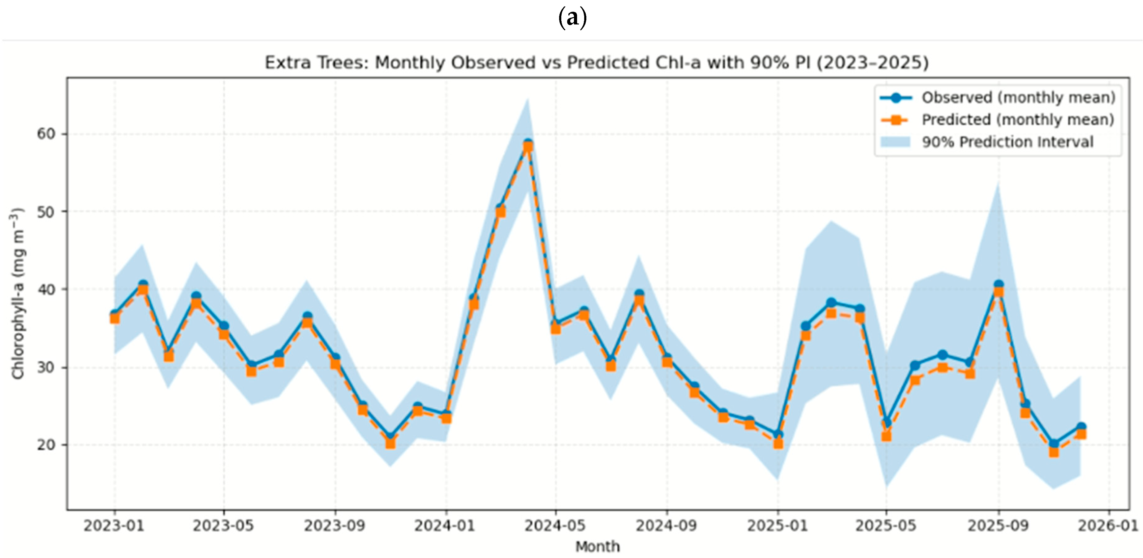
Uncertainty was quantified for both Extra Trees (ET) and XGBoost to evaluate the reliability of model predictions. For the ET model, prediction intervals were derived by leveraging variability among individual tree predictions rather than relying solely on the ensemble mean [63]. For each test sample, predictions from all trees were extracted in log-transformed space, and the ensemble mean together with the 5th and 95th percentiles was used to construct a 90% prediction interval (PI90). These bounds were then back-transformed to the original Chl-a concentration scale using the inverse log(1 + x) transformation. The resulting interval width (PI_upper − PI_lower) serves as a pixel-level measure of predictive uncertainty. The ET model achieved a PI90 coverage of approximately 0.843, with a mean interval width of 11.64 mg m⁻³ and a median width of 6.61 mg m⁻³, indicating relatively narrow intervals with moderate coverage. In contrast, uncertainty for the XGBoost model was estimated using a residual-based approach, where the 90th percentile of absolute training residuals was used to construct symmetric prediction intervals. This approach enables uncertainty estimation for boosting-based models that do not inherently provide per-tree variability. The XGBoost model achieved a PI90 coverage of approximately 0.905, closely matching the nominal 90% level and indicating well-calibrated uncertainty. 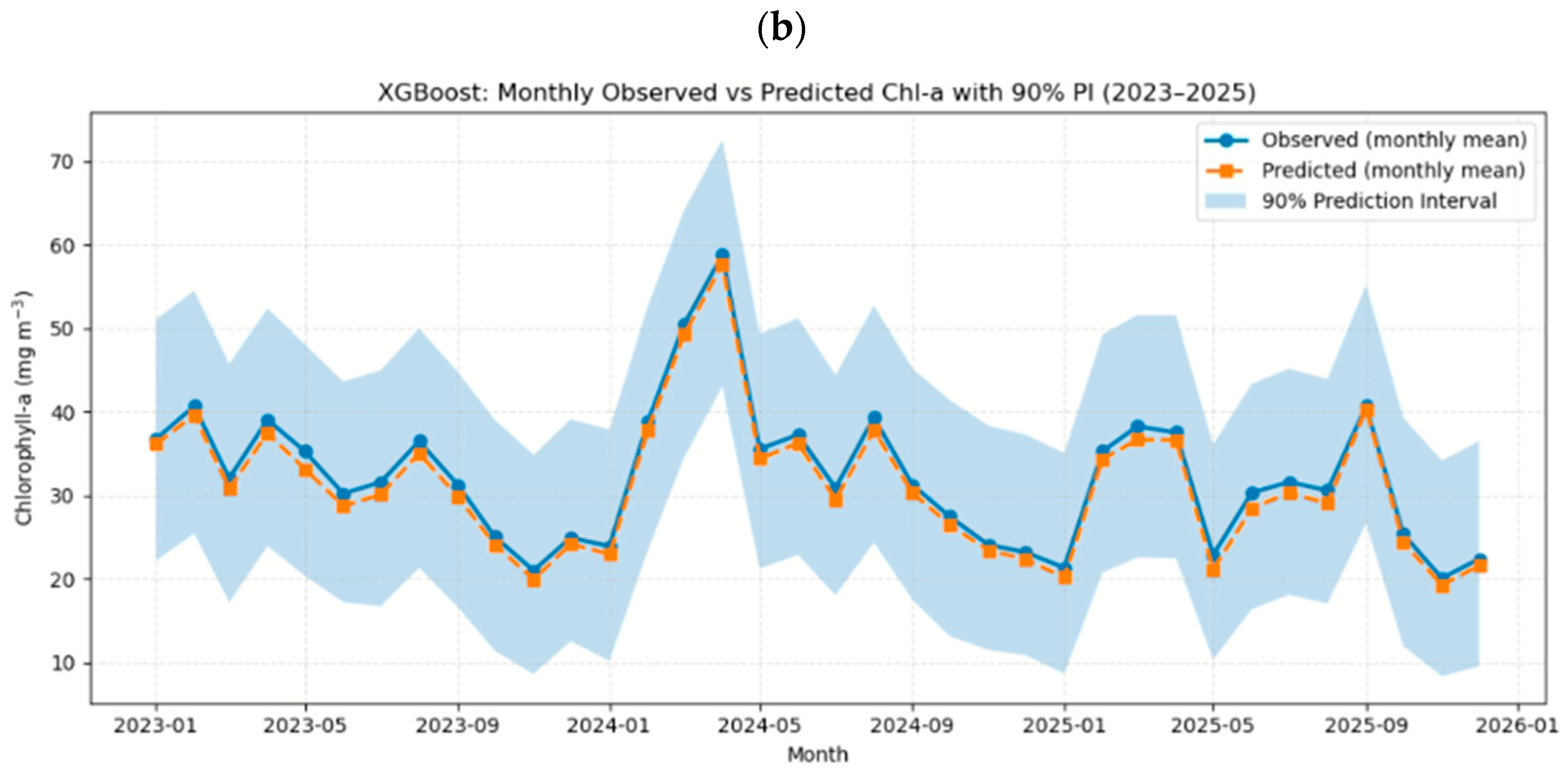However, the larger mean interval width (27.26 mg m⁻³) reflects a more conservative uncertainty estimate relative to ET. The comparison between the two models highlights an important trade-off between interval width and reliability. The ET model produces narrower intervals but underestimates uncertainty, as indicated by its lower coverage. In contrast, XGBoost provides wider but better-calibrated intervals, ensuring that a higher proportion of true observations fall within the predicted bounds. Monthly aggregation of uncertainty is illustrated in Figure 9. The blue solid line represents the monthly mean observed Chl-a for the held-out testing subset, while the orange dashed line shows the corresponding monthly mean predictions. The shaded region denotes the monthly mean 90% prediction interval. Temporal widening of the band indicates periods of elevated uncertainty, typically associated with rapid seasonal transitions. When observed values fall outside the shaded region, the model underestimates uncertainty during those intervals.

Overall, these results indicate that XGBoost provides more reliable and well-calibrated uncertainty estimates, whereas ET produces tighter but less conservative bounds.

6. Discussion

6.1. Interpretation of Model Behavior

The variation in model behavior is largely influenced by how each approach represents relationships within spatiotemporal environmental data. Methods that depend on local similarity, such as IDW and KNN, perform well under conditions of dense and uniformly distributed observations but degrade in performance as data become sparse or highly variable. This limitation is particularly pronounced in the Chesapeake Bay, especially near river-influenced regions and coastal boundaries, where chlorophyll concentrations exhibit rapid spatial changes and increased heterogeneity. Previous studies have shown that DINEOF is effective for reconstructing missing Chl-a observations by capturing dominant spatial–temporal variability patterns in satellite datasets [22]. In the present study, DINEOF provided stable large-scale reconstruction under high missing-data conditions, although its performance remained lower than the supervised machine-learning and convolutional autoencoder approaches in representing localized nonlinear variability within the Chesapeake Bay. In contrast, ensemble-based models are better suited to such conditions, as they integrate multiple decision rules to capture complex interactions among spatial, temporal, and neighborhood features. This enables greater adaptability to heterogeneous coastal water quality patterns. This pattern is consistent with prior studies in the Chesapeake Bay, where Extra Trees models applied to long-term satellite datasets reported R² values in the range of 0.475–0.581 [15]. By comparison, the Extra Trees model in this study achieved an R² of 0.850, indicating substantial performance improvement under the proposed spatiotemporal gap-filling framework. This improvement likely arises from the incorporation of spatiotemporal predictors and temporal lag features, which better represent local variability and seasonal dynamics. In contrast, approaches relying primarily on spectral reflectance inputs may be more sensitive to noise and less effective under high missing-data conditions.

The advantage of boosting-based learning lies in its ability to iteratively refine predictions by focusing on previously misrepresented patterns. This results in improved representation of localized variability, particularly in regions where chlorophyll concentrations change rapidly. Bagging-based methods, while effective in reducing variability through averaging, do not incorporate this stepwise correction process, which can limit their sensitivity to subtle or abrupt changes. As a result, different ensemble strategies lead to differences in how well small-scale features and transitions are represented. Similar findings have been reported in recent studies using XGBoost for Chl-a prediction [54], where R² values of up to 0.99 have been achieved for short-term (1-day) forecasting tasks. In the present study, XGBoost achieved the best performance among the evaluated models (R² = 0.86), demonstrating strong capability in reconstructing missing satellite observations. This performance is likely driven by its ability to iteratively learn from residual errors using structured spatiotemporal inputs. In contrast, forecasting-based studies typically assume continuous observations, whereas the present framework explicitly addresses the more challenging problem of reconstructing missing satellite data under incomplete observation conditions. Another important aspect is the balance between stability and sensitivity in model predictions. Techniques that emphasize stability tend to produce smoother outputs, which helps reduce noise but may also soften sharp gradients or extreme values. This behavior reflects a general trade-off in machine learning models applied to environmental data, where capturing fine-scale variability must be balanced against maintaining consistent and reliable predictions. In this context, the ability to preserve meaningful patterns while avoiding instability is more critical than reproducing every extreme value exactly. Similar patterns have been reported in deep-learning studies [64], where LSTM-based models achieved R² values of approximately 0.52 under independent testing conditions, reflecting challenges in generalization across varying environments. In the present study, the LSTM model achieved an R² of 0.834, indicating strong temporal learning capability and improved predictive performance. This improvement is likely attributable to the incorporation of continuous time-series information through lag-based inputs, which strengthens temporal representation and enhances prediction consistency. In contrast, prior studies often rely on models trained and evaluated at single monitoring locations, whereas the present study utilizes spatially distributed data across the Chesapeake Bay, enabling the model to capture both spatial heterogeneity and temporal variability within the study region. The Temporal DINCAE framework also demonstrated competitive reconstruction performance, although slight underestimation was observed under higher chlorophyll-a conditions.

Overall, these findings emphasize the importance of selecting models that align with both data characteristics and application requirements. In satellite-based monitoring, where observations are frequently incomplete and influenced by environmental variability, effective models must preserve coherent spatial–temporal patterns while adapting to dynamic conditions. Boosting-based approaches are therefore particularly well suited for reconstructing satellite-derived environmental variables characterized by nonlinear spatiotemporal complexity and high missing-data fractions.

6.2. Limitations

This study can be extended in several directions to enhance both its scientific rigor and operational applicability. Because the reconstruction relies solely on satellite-derived observations, errors associated with atmospheric correction and retrieval algorithms may propagate into the modeling process and influence prediction accuracy.

Although the current framework is evaluated within the Chesapeake Bay, its transferability to other coastal and estuarine systems should be systematically assessed. Applying the methodology across regions with differing hydrological regimes, optical properties, and nutrient dynamics would provide insight into model generalizability and robustness under diverse environmental conditions. Future work should also incorporate multi-sensor data integration, including Sentinel-2, MODIS, and VIIRS observations, to improve temporal density and cross-platform consistency [65]. Such integration may help reduce cloud-induced gaps and improve reconstruction stability across varying spatial resolutions.

In this study, validation using field observations is subject to several sources of uncertainty. Although satellite and in situ data were matched on the same day, chlorophyll-a concentrations in coastal waters can vary over short time scales, resulting in temporal mismatches between satellite overpass and field sampling [66]. Moreover, satellite observations represent spatial averages over grid cells, whereas in situ measurements are collected at discrete points, leading to scale mismatches that may reduce agreement. These effects are particularly pronounced in heterogeneous environments such as the Chesapeake Bay, where water properties exhibit rapid spatial variability. In addition, suspended sediments and colored dissolved organic matter can affect the optical signal, complicating the retrieval of chlorophyll-related information from satellite data. Consequently, both observed and reconstructed values may exhibit systematic bias and reduced correlation with field measurements. It is important to emphasize that the reconstruction framework is designed to enhance spatial and temporal continuity rather than optimize point-level accuracy. Accordingly, in situ comparisons should be interpreted as a consistency check rather than a direct evaluation of model performance at individual locations.

Finally, uncertainty quantification could be expanded through calibrated probabilistic frameworks, such as conformal prediction, quantile regression forests, or Bayesian ensemble methods. A more rigorous treatment of predictive uncertainty would enhance decision-support reliability and strengthen the operational deployment potential of the proposed reconstruction framework.

7. Conclusions

This study examined how different approaches, including baseline interpolation, machine learning, and deep learning, can be used to fill missing Chl-a values in satellite data to improve harmful algal bloom monitoring in the Chesapeake Bay. Cloud cover often creates gaps in satellite observations, which makes it difficult to track water quality continuously. To address this issue, a baseline interpolation method IDW, four machine learning models—K-Nearest Neighbors, Random Forest, Extra Trees, and XGBoost—and a deep learning model LSTM were tested using Sentinel-3 OLCI data for 2025. The results show that all models were able to reproduce the general seasonal pattern of chlorophyll levels. The IDW method provided a simple baseline but showed limited accuracy under complex spatial conditions. Among the machine learning models, XGBoost produced the most accurate results and showed the best ability to estimate missing values. Random Forest and Extra Trees also performed well and gave stable predictions across different conditions. In comparison, the KNN model showed slightly lower accuracy because it relies mainly on nearby data points. The LSTM model demonstrated strong capability in reducing prediction error by capturing temporal dependencies, highlighting the importance of incorporating time-based information in gap-filling tasks. The reconstructed results preserve both the seasonal variability and spatial distribution of chlorophyll across the Chesapeake Bay. Some peak bloom values were slightly underestimated, but the overall understanding between observed and predicted values remained strong. In addition, uncertainty quantification was performed using both Extra Trees and XGBoost. The results showed that XGBoost provided well-calibrated uncertainty estimates with coverage close to the expected level, while Extra Trees produced narrower intervals but tended to underestimate uncertainty. This comparison highlights the importance of selecting appropriate uncertainty methods for reliable model deployment. Overall, the results show that tree-based machine learning models and sequence based deep leaning model can provide reliable solutions for filling gaps in satellite water-quality data. By improving the completeness of chlorophyll datasets, this approach can support more consistent monitoring of harmful algal blooms. The framework developed in this study is simple, reproducible, and suitable for large satellite-scale environment applications. In the future, combining multiple satellite sources and field observations could further improve the accuracy of the reconstruction. This would make satellite-based monitoring more reliable for environmental studies and water-quality management.