Hyperspectral and Multispectral Image Fusion Based on Adaptive Wavelet Transform and Dual Spectral–Spatial Branch

Highlights

What are the main findings?

• A wavelet-deep learning hybrid fusion framework is proposed, which combines pixel-wise adaptive wavelet, transform with dual-branch spectral–spatial feature extraction, effectively preserving spectral fidelity and spatial details.
• By introducing an adaptive wavelet transform gating mechanism and cross-scale cross-domain bidirectional attention, dynamic optimization of wavelet basis functions and efficient collaboration between features are achieved, thereby significantly improving reconstruction performance.

What are the implications of the main findings?

• Experimental results show that the proposed method can effectively alleviate the information loss and fusion errors caused by resolution mismatch, providing a robust and well-generalizable paradigm for hyperspectral-multispectral fusion.
• Experimental results show that the proposed method exhibits strong application performance and provides effective support for downstream tasks such as semantic segmentation and precision agriculture.

Abstract

As the role of remote sensing continues to grow, the fusion technology of low-spatial-resolution hyperspectral images and high-spatial-resolution multispectral images has become increasingly critical. Traditional methods rely on fixed rules and exhibit poor robustness, whereas deep learning methods struggle to establish efficient interactions between local and global information due to the complexity of their underlying networks. Therefore, we propose a deep learning fusion module that combines pixel-wise adaptive wavelet transform with a spectral–spatial dual-branch extraction. Firstly, by utilizing the unique properties of the wavelet transform, it is possible to effectively preserve spectral information and extract spatial edge features, thereby achieving preliminary fusion by leveraging both low-frequency and high-frequency components. To compensate for the lack of nonlinear expression capability in the wavelet transform, a dual-branch parallel extraction of spectral and spatial features is subsequently performed in the deep learning module. The Multi-Scale Group Convolution module (MSGC) is utilized to extract spectral information, while the Spectral Compression and Spatially Guided Gating Module (SCSGM) is employed to extract spatial information, thereby enhancing the data’s adaptive capability. A bidirectional attention mechanism is interspersed within the module to capture complementary information across different scales, ultimately reconstructing a high-resolution hyperspectral image. Finally, the proposed fusion strategy demonstrates superior performance in practical image reconstruction, outperforming more than ten state-of-the-art fusion methods.

1. Introduction

In the field of remote sensing, numerous studies have shown that hyperspectral imagery [1] plays a crucial role in multiple domains, such as agriculture and geological exploration [2,3]. However, due to the limitations of hyperspectral imaging technology [4], hyperspectral images have relatively low spatial resolution. In contrast, multispectral images (MSI) usually possess higher spatial resolution but contain fewer spectral channels (e.g., RGB). Therefore, many studies have employed various technical approaches to fuse these two modalities, aiming to exploit their complementary advantages.

Modern hyperspectral satellites, such as PRISMA and HYPERION [1], have relatively low spatial resolution. Thus, directly applying their data to fields such as geological exploration [3], biomass inversion [2,5], and agricultural monitoring [6] often results in reduced or insignificant performance. In forest resource surveys and ecological monitoring, the accuracy of existing tree species distribution maps remains limited, and a single remote sensing data source is often insufficient to fully characterize the differences among forest types. Since large-scale field surveys are costly and slow to update, multi-source remote sensing data fusion and machine learning methods have been used to improve tree species identification and distribution mapping capabilities [7]. This limitation is particularly critical in mainstream tasks, such as object detection [8], change detection [9,10], and land-cover classification [11,12,13], where the rich spectral information in HSI is indispensable. Current research trends have shifted from purely improving imaging hardware toward deep learning–based fusion methods [10,14]. These methods integrate LR-HSI with HR-MSI to obtain high-resolution HR-HSI with both high spectral and spatial fidelity.

In traditional methods, multi-resolution analysis (MRA) techniques, such as the Laplacian pyramid [15], extract high-frequency spatial details from MSI and inject them into upsampled HSI to enhance spatial resolution. However, such high-frequency injection is typically based on simple addition or ratio transfer, which lacks spectral consistency and leads to spectral distortion. Statistical and matrix-based methods, such as principal component analysis [16], tensor decomposition [17,18], and nonnegative matrix factorization (NMF) [19,20], utilize the low-rank property of HSI to project MSI’s spatial information into the spectral domain for representation, reconstructing spectra via low-rank coefficients [21,22]. These linear mathematical models, however, struggle to establish complex nonlinear spectral relationships, require high computational costs, and depend heavily on training data. Wavelet transform–based methods [23,24,25] perform multi-scale analysis by replacing low-frequency and high-frequency components and conducting fusion in the frequency domain via inverse transformation. However, their performance depends heavily on the choice of wavelet basis [26], limiting their generalizability. Prior-knowledge-based fusion [27] maintains spectral or spatial consistency through constraints, offering good interpretability and overall performance but relying on idealized assumptions and manual parameter tuning. These iterative algorithms have high computational costs, weak generalization, and the risk of local minima.

Pan-sharpening-based methods [28,29,30] usually enhance spatial details by fusing panchromatic images with multispectral data, offering the advantages of simple implementation and effective spatial sharpening. However, these methods are prone to spectral distortion, physical inconsistency, and noise sensitivity, which limit their application in hyperspectral image fusion and further promote the development of deep learning-based fusion methods [31]. Meanwhile, in hyperspectral full-band sharpening tasks, maintaining consistent spectral quality across different bands remains an important challenge. Recent research [32] has improved spatial sharpening quality and spectral fidelity without relying on external training data by introducing zero-shot unsupervised training, a band-adaptive lightweight network, and a hysteresis-based loss tuning strategy, providing new insights for hyperspectral image fusion research.

In recent years, the rapid rise of convolutional neural networks (CNNs) [14] has made deep learning a key technology across various fields. CNNs [33] extract features such as textures and edges through local convolution kernels and multi-level architectures [34], effectively capturing spatial detail. Modern deep fusion networks [35] employ activation functions and multi-layer structures to learn complex nonlinear mappings between spectral and spatial domains. However, CNNs have difficulty effectively utilizing spatial positional information and modeling long-range dependencies, leading to a loss of global contextual information. On this basis, the Transformer [36] has emerged with its unique self-attention mechanism, which models associations between features at any position. It is particularly suitable for capturing long-range dependencies across spatial and spectral dimensions, thereby solving the spectral inconsistency and global structure misalignment caused by the limited receptive fields of CNNs [37]. However, Transformers still suffer from high computational complexity and dependence on large-scale training data.

This paper proposes a hybrid framework that integrates traditional methods with deep learning for hyperspectral and multispectral image fusion, aiming to efficiently model the nonlinear correspondence between spectral and spatial information and significantly improve reconstruction accuracy. Traditional wavelet-based methods typically use fixed basis functions and decomposition levels, making them inadequate for complex scenarios. To address this limitation, this study introduces an adaptive spectral decomposition approach based on learnable wavelet bases. Specifically, 1D wavelet transforms are utilized to extract spectral features, while 2D wavelet transforms capture spatial features. By reconstructing candidate wavelet bases and applying a Softmax-based gating mechanism, the model performs pixel-wise adaptive weighting, enabling each pixel to select the optimal wavelet basis automatically. A learnable “soft selection combine lightweight scaling” strategy is further employed to enhance flexibility in spectral decomposition while maintaining interpretability and stability. End-to-end optimization jointly trains wavelet selection and the fusion objective, yielding task-specific optimal solutions.

In the downstream fusion stage, a multi-scale grouped convolution module (MSGC) is introduced to overcome the limited receptive field of single convolutions. This module employs parallel grouped convolutions at different scales to capture multi-granular texture information under spatial constraints, achieving both detail enhancement and spectral fidelity. Grouped spectral modeling strengthens texture discrimination, reduces channel redundancy, and improves network trainability and generalization.

Moreover, the Transformer’s self-attention mechanism struggles to learn cross-modal relationships. To address this, a cross-attention mechanism is incorporated into the spatial and spectral branches to achieve complementary alignment between MSI and HSI. The bidirectional attention effectively eases gradient propagation and reduces feature redundancy, which are issues found in conventional residual structures. The framework strikes a balance between computational efficiency, interpretability, robustness, and high performance.

The main contributions of this paper are summarized as follows:

• We propose a parallel architecture that leverages a 1D wavelet transform for spectral dimension extraction and a 2D wavelet transform for spatial dimension extraction, respectively. A Softmax gating mechanism is designed to adaptively select wavelet basis functions for each pixel based on varying weight distributions, which enhances the frequency-domain modeling capability. This framework fully preserves the spectral and spatial information across different bands, leading to a significant improvement in both image quality and fusion accuracy.
• A multi-scale grouped convolution module (MSGC) is designed for spectral feature extraction. It expands the receptive field and strengthens inter-group interaction while reducing computational cost and parameter redundancy.
• A Bidirectional attention mechanism (BiDAttention) is introduced to enable long-range interaction with the original information. By integrating local and global features, it enhances fusion quality while maintaining image completeness and fidelity.
• A spatial feature extraction module (SCSGM) is developed, employing multiple gating systems to dynamically and adaptively select features during computation. This design strengthens spatial texture representation and highlights edge and structural information.

The remainder of this paper is organized as follows: Section 2 reviews related work on traditional and deep learning–based methods. Section 3 provides a detailed description of the proposed model, clarifying the theoretical basis and implementation steps of model construction. Section 4 presents the experimental results on four benchmark datasets, along with discussions and an ablation study analysis of each module. Finally, Section 5 concludes the paper.

2. Related Works

2.1. Traditional Methods

Traditional fusion methods mainly include approaches based on the concept of pan-sharpening [28,30], which aim to inject high-spatial-detail information from MSI into HSI while addressing the significant spectral discrepancies between the two modalities. Aly et al. [38] proposed a regularized model framework utilizing matrix factorization, where the image is decomposed into a basis matrix and a coefficient matrix. By constraining and partially replacing the coefficients, endmember and abundance matrices are extracted to reconstruct high-resolution hyperspectral images (HR-HSI). Yokoya et al. [5] introduced the Coupled Nonnegative Matrix Factorization (CNMF) method, which jointly decomposes the images into mixed pixels using coupled NMF. By leveraging the abundance matrix from LR-HSI and the endmember matrix from HR-MSI, an alternating unmixing strategy is applied to enhance spatial resolution while maintaining spectral fidelity. For tensor-based approaches, Xu et al. [39] proposed a coupled Tucker tensor decomposition framework that captures the inherent spectral–spatial structure during the fusion process. This method enhances fusion accuracy by sharing spectral–spatial factor matrices across modalities, albeit at the expense of significantly increased computational complexity.

Wavelet-based methods use predefined wavelet bases to extract frequency-domain components. Chakkarwar et al. [40] combined wavelet decomposition with nonlinear IHS transformation to mitigate spectral distortion. However, traditional wavelet transforms suffer from fixed basis functions and limited directional representation, leading to poor adaptability across diverse scene types.

Although traditional methods can yield satisfactory results under specific conditions, their performance heavily depends on manually designed prior information [41]. These methods typically incur high computational costs and exhibit limited generalization capabilities. When applied to complex and dynamic real-world surfaces, such simplified models fail to capture the intrinsic complexity of hyperspectral data, often resulting in spectral distortion or spatial artifacts in the fusion outputs.

2.2. Deep Learning Methods

Deep learning methods enable end-to-end learning of complex nonlinear relationships between HSI and MSI. The Transformer architecture, proposed by Vaswani et al. [42], adopts a self-attention mechanism to capture long-range pixel dependencies. Its flexible tokens can handle the receptive field between local and global regions, providing a powerful framework for integrating contextual information and improving the feature representation capability.

Shi et al. [43] proposed the Hierarchical Spatial–Spectral Transformer (HSST), which combines local and global contextual modeling. Through cross-attention and multi-scale feature extraction, HSST refines spatial details during upsampling, resulting in superior reconstruction accuracy. Zhao et al. [44] developed a spatial–spectral interactive CNN–Mamba fusion network that enables bidirectional guidance between MSI and HSI. The method enhances both spectral consistency and spatial clarity, achieving high-quality HR-HSI reconstruction through joint feature learning. Li et al. [45] introduced a Multi-scale Inception-Mixed Transformer (MIMFormer) that fuses hierarchical local–global features across spectral groups, allowing richer detail representation and more comprehensive spatial–spectral fusion. Wang et al. [46] proposed FSL-Unet, a full-scale U-Net–based architecture using a Spatial–Spectral Joint Perception Attention (SSJPA) mechanism. By integrating encoder–decoder skip connections, the network effectively filters redundant features and reconstructs fine-grained spatial structures with high precision. Li et al. [47] designed the FCSwinU network, combining a Spectral Fast Fourier Convolution (SFFC) module for efficient spectral feature extraction with a self-attention block for global feature fusion. This U-Net–based architecture successfully balances spatial fidelity and spectral precision, outperforming conventional CNN models. Dai et al. [48] proposed a multi-scale channel attention module with an iterative attention-based fusion strategy to better handle inconsistent semantics across scales, thereby achieving stable optimization and robust fusion. Zhang et al. [49] introduced the interpretable Spatial and Spectral Reconstruction Network (SSR-Net), which incorporates spatial and spectral edge losses to guide the reconstruction process, thereby significantly improving both fidelity and interpretability.

Ke Zheng et al. [50] proposed an Unsupervised Pretraining Fusion Framework (UPFW), where a low-resolution supervised pretraining phase learns degradation parameters, followed by unsupervised full-resolution fusion, improving adaptability and generalization. Liu et al. [51] developed UMAG-Net, an unsupervised multi-attention network that extracts multi-scale deep features and learns prior knowledge through iterative HSI–MSI reconstruction losses, resulting in stable fusion outcomes. Cao et al. [52] proposed an unsupervised Transformer-based network (UMSFT), which performs multi-level spatial–spectral feature fusion and incorporates spectral-domain cross-attention to model global spatial–spectral correlations within an unsupervised framework, thereby reducing fusion distortions. Jia et al. [53] proposed an unsupervised deep pretraining fusion framework that utilizes spectral–spatial collaborative constraints with adaptive inverse-mapping modules, thereby effectively enhancing joint feature extraction and fusion.

Deng et al. [54] introduced the Pyramid Shuffle and Reshuffle Transformer (PSRT), which integrates a window-based attention mechanism and a pyramid multi-scale design, significantly improving fusion accuracy and adaptability to varying resolutions. Wang et al. [55] introduced the Multi-level Cross Transformer (MCT-Net), which fuses cross-modal information through hierarchical interaction and aggregation modules to achieve deep, scale-consistent spectral–spatial fusion. Y. He et al. [56] proposed a his–MSI fusion method based on the Retrenchable Spatial–Spectral Transformer Network (RSST), which introduces the retrenchable attention mechanism into remote sensing image fusion and employs a gradient spatial–spectral recovery module to alleviate the limitations of token interaction and the loss of spatial–spectral edge information.

Cao et al. [57] proposed a cross-domain perception Transformer (CaFormer) within a deep unfolding framework, which models intrinsic HSI dependencies via unified cross-domain representation and spatial–spectral joint attention, further enhanced by frequency-domain perception and a two-stage prior transfer strategy. Ma et al. [58] introduced a reciprocal Transformer (DCTransformer) that employs bidirectional cross-modal multi-head cross-attention along with self-attention to facilitate information exchange and contextual modeling, thereby improving hyperspectral–multispectral fusion performance.

2.3. Wavelet Dictionary

Donoho [59] theoretically established the near-optimality of wavelet soft-thresholding shrinkage for signal denoising, providing a solid statistical foundation for sparse representation and multiscale decomposition. Daubechies wavelets [60], characterized by compact support and orthogonality, enable sparse signal representation and efficient reconstruction. Li et al. [61] further demonstrated the effectiveness of the wavelet framework in multispectral image fusion, showing its ability to enhance spatial details while suppressing spectral distortion, thus supporting spatial–spectral collaborative modeling in hyperspectral–multispectral fusion.

Symlets [60], as approximately symmetric extensions of Daubechies wavelets, improve symmetry while preserving compact support, thereby enhancing edge preservation and reducing oscillation artifacts. Zhang et al. [62] verified the advantages of symmetric wavelets in maintaining spatial structures, indicating their potential for edge-detail restoration in hyperspectral fusion.

Coiflets [63], featuring higher-order vanishing moments and strong energy compaction, are grounded in entropy-based optimal basis selection theory. Chang et al. [64] demonstrated that sparsity-driven transforms with strong spectral separation properties effectively preserve spectral consistency, highlighting the advantages of Coiflets in spectral feature representation.

In addition, biorthogonal wavelets (e.g., the 9/7 wavelet adopted in JPEG2000) possess linear-phase and symmetric reconstruction properties [65,66], and have been widely applied in high-fidelity image reconstruction and compression. Starck et al. [67] further emphasized their effectiveness in structural preservation and detail representation from a sparse and multiscale perspective.

Overall, different wavelet bases exhibit complementary properties in spatial structure preservation, spectral consistency maintenance, and energy compaction. These characteristics form a theoretically grounded and compact multiscale dictionary for adaptive hyperspectral–multispectral image fusion, enabling enhanced spatial detail reconstruction while mitigating spectral distortion.

3. Method

In this section, we describe the proposed AWD-Net. We begin with an overview of its workflow. Next, we give a detailed explanation of its core components.

3.1. Overall Framework

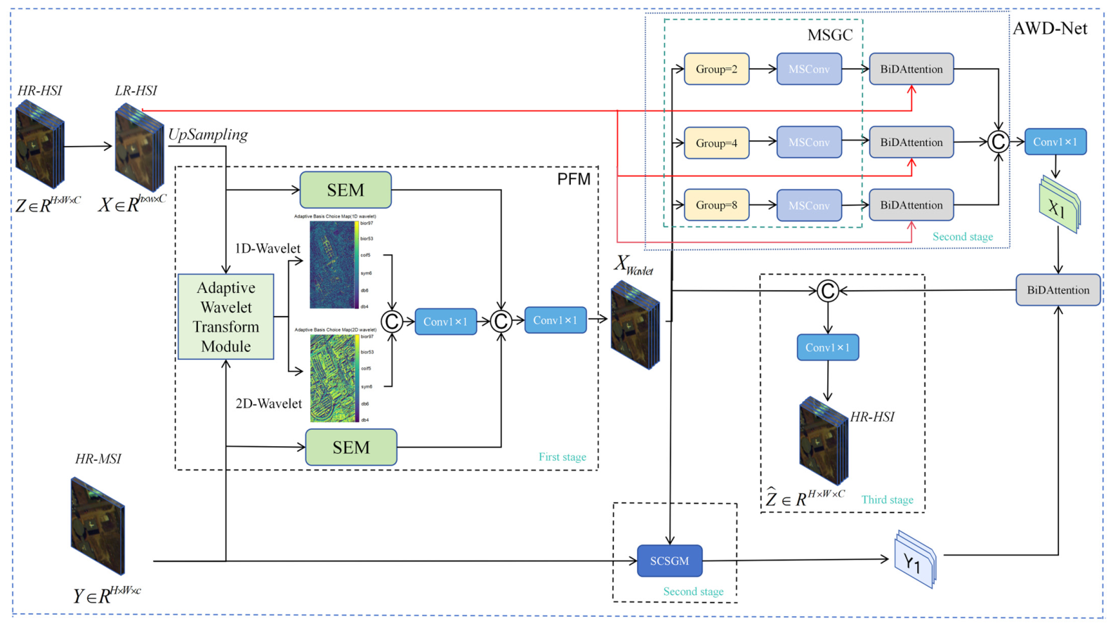
As illustrated in Figure 1, the proposed AWD-Net fusion framework comprises four core modules: Preliminary Fusion Model (PFM), the Bidirectional Attention Mechanism, the Spectral Feature Extraction module, and the Spatial Feature Extraction module. It is a deep fusion network framework that integrates the preliminary fusion of the wavelet transform in the front and dual-branch extraction for deep fusion.

In our AWD-Net model, the first stage comprises a preliminary fusion module that combines shallow feature extraction with parallel 1D and 2D wavelet transforms, enabling frequency domain extraction and spatial domain reconstruction.

In the second stage, a deep learning framework with dual spatial–spectral branches is constructed. For spectral feature extraction, convolutional layers combined with a cross-scale bidirectional attention mechanism are employed to capture long-range dependencies. For spatial feature extraction, a dual-input structure is adopted to perform spectral compression and form a spatial-guided gating mechanism, thereby enhancing the fine representation of detailed features.

In the third stage, the preliminarily fused features are concatenated along the channel dimension, followed by convolution to restore them to the original dimensionality, ultimately producing the final HR-HSI output.

A high-spatial-resolution hyperspectral image can be mathematically expressed as $Z\in {ℝ}^{\mathrm{B}\times \mathrm{C}\times \mathrm{H}\times \mathrm{W}}$. The input LR-HSI is $X\in {ℝ}^{\mathrm{B}\times \mathrm{C}\times \mathrm{h}\times \mathrm{w}}$ ($\mathrm{h}\ll \mathrm{H},\mathrm{w}\ll \mathrm{W}$) and HR-MSI is $Y\in {ℝ}^{\mathrm{B}\times \mathrm{c}\times \mathrm{H}\times \mathrm{W}}$ ($\mathrm{c}\ll \mathrm{C}$). Our ultimate objective is to obtain the super-resolved hyperspectral image by fusing X and Y via the proposed framework: $\widehat{Z}\in {ℝ}^{\mathrm{B}\times \mathrm{C}\times \mathrm{H}\times \mathrm{W}}$ (h and H denote the number of rows, w and W denote the number of columns, and c and C denote the number of spectral bands).

In this method, the LR-HSI is first upsampled using bilinear interpolation to obtain $X_{\mathrm{up}}\in {ℝ}^{\mathrm{B}\times \mathrm{C}\times \mathrm{H}\times \mathrm{W}}$ in order to align its dimensions with the HR-MSI for subsequent computations.

This process can be mathematically expressed as:

$$X_{\mathrm{up}}=\mathrm{Upsampling}(X).$$

(1)

where $\mathrm{Upsampling}(•)$ denotes the bilinear interpolation function.

Finally, to ensure fusion quality, we adopt the Mean Squared Error loss function as the training loss of the network.

$${\mathcal{L}}_{\mathrm{MSE}}={\displaystyle \frac{1}{\mathrm{BCHW}}}\left|\right|\widehat{Z}-G|{|}_F^2,G\in {ℝ}^{\mathrm{B}\times \mathrm{C}\times \mathrm{H}\times \mathrm{W}}.$$

(2)

where $G$ and $\widehat{Z}$ represent the ground truth and reconstructed images, respectively. The following sections will provide a detailed introduction to PFM, MSGC, SCSGM, and BiDAttention, respectively.

3.2. Preliminary Fusion Model (PFM)

3.2.1. Shallow Feature Extraction (SEM)

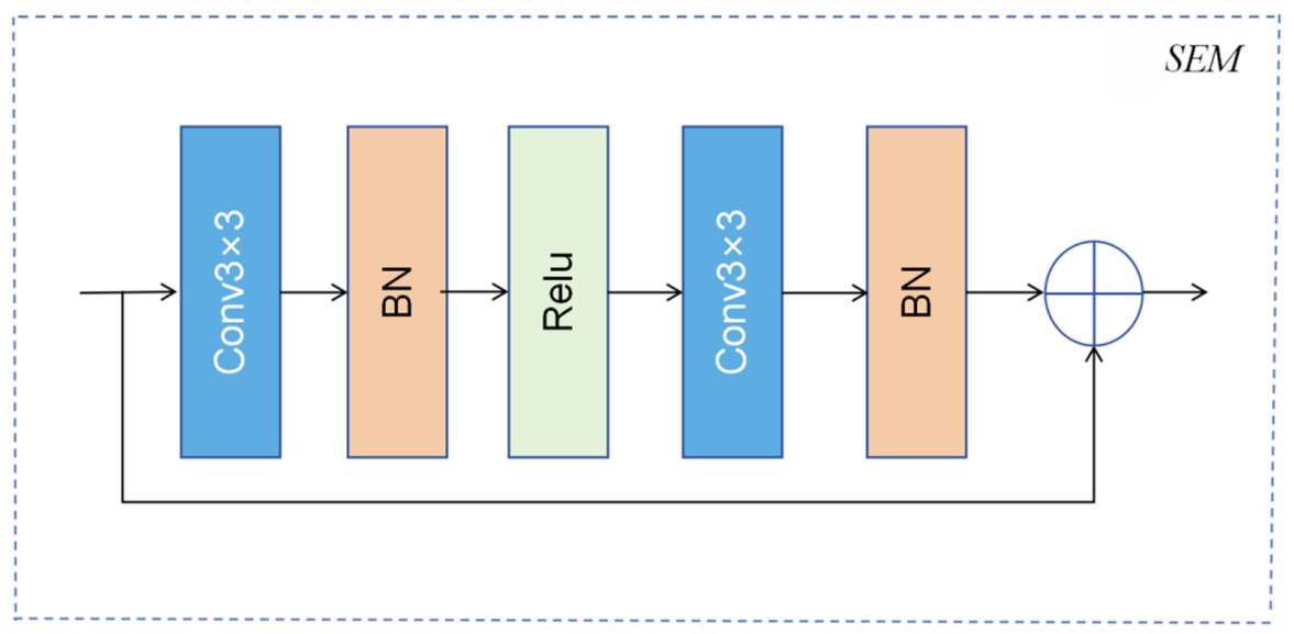
As shown in Figure 2, the SEM module primarily comprises convolutional layers, layer normalization, and activation functions, with a residual connection. A learnable scaling parameter $\alpha$ (initially set to 0.2) is introduced to prevent the residual term from being excessively amplified. During subsequent training, this parameter is updated through back-propagation, stabilizing gradient propagation and feature responses.

The formulation of the SEM can be expressed as:

$$X_{\mathrm{SEM}}=X+\mathsf{\alpha }\mathrm{B}{\mathrm{N}}_2({\mathrm{Conv}}_{3\times 3}(\mathsf{\sigma }(\mathrm{B}{\mathrm{N}}_1({\mathrm{Conv}}_{3\times 3}(X))))).$$

(3)

3.2.2. Adaptive Wavelet Transform Module (AWTM)

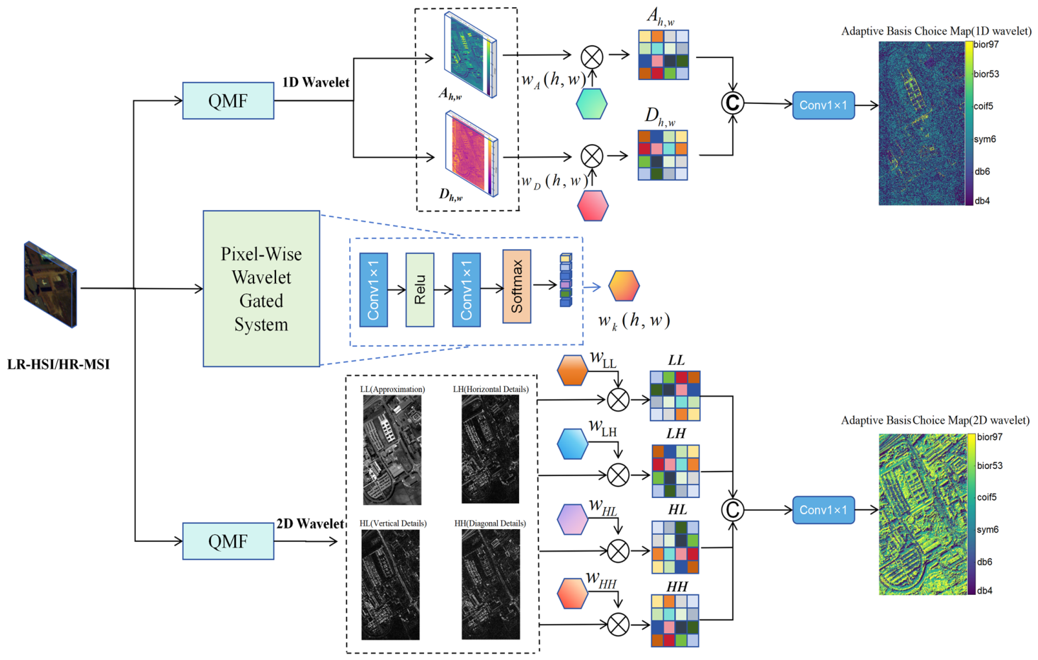
The overall workflow is shown in Figure 3. The 1D wavelet extraction in the spectral dimension and 2D wavelet extraction in the spatial dimension can be expressed by the following mathematical formulas:

$$X_{1\mathrm{D}}=\mathrm{Wavele}{\mathrm{t}}_{1\mathrm{D}}(X_{\mathrm{up}}).$$

(4)

$$X_{2\mathrm{D}}=\mathrm{Wavele}{\mathrm{t}}_{2\mathrm{D}}(Y).$$

(5)

• 1D wavelet

For the 1D wavelet transform, the spectral vector of each pixel in the HSI can be represented as:

$$x_{\mathrm{h},\mathrm{w}}={[{\mathrm{x}}_1,{\mathrm{x}}_2,\dots ,{\mathrm{x}}_{\mathrm{C}}]}^{\mathrm{T}}\in {ℝ}^{\mathrm{C}}.$$

(6)

where C denotes the number of spectral channels.

By performing a 1D wavelet Transform on the spectral vector $x_{\mathrm{h},\mathrm{w}}$, we use Quadrature Mirror Filters (QMFs) to generate two-component features for each pixel.

$$A_{\mathrm{h},\mathrm{w}}=x_{\mathrm{h},\mathrm{w}}\ast L{o}_{\mathrm{k}},$$

(7)

$$D_{\mathrm{h},\mathrm{w}}=x_{\mathrm{h},\mathrm{w}}\ast H{i}_{\mathrm{k}},$$

(8)

where $A_{\mathrm{h},\mathrm{w}}$ and $D_{\mathrm{h},\mathrm{w}}$ represent the low-frequency and high-frequency coefficients, respectively, and $L{o}_{\mathrm{k}},H{i}_{\mathrm{k}}$ denote the corresponding low-pass and high-pass filters. The low-frequency component effectively captures the smooth spectral shape, whereas the high-frequency component preserves sudden spectral variations and fine details, such as absorption peaks.

For these two filters, the sum of their squared magnitude responses at any frequency ω equals 1, leading to the following constraint: $|\mathrm{L}{\mathrm{o}}_{\mathrm{k}}(\mathsf{\omega }){|}^2+|\mathrm{H}{\mathrm{i}}_k(\mathsf{\omega }){|}^2=1$. In the QMF framework, the two filters also satisfy the quadrature mirror relationship, which can be written as

$$\mathrm{H}{\mathrm{i}}_{\mathrm{k}}\left[\mathrm{n}\right]={(-1)}^{\mathrm{n}}\cdot \mathrm{L}{\mathrm{o}}_{\mathrm{k}}[\mathrm{L}-1-\mathrm{n}]$$

(9)

where L denotes the filter length.

2.

2D wavelet

Through low-pass and high-pass filters, the image is decomposed into four subbands, namely LL, LH, HL, and HH. The mathematical expressions of these four subbands are as follows:

$$\mathrm{LL}(\mathrm{i},\mathrm{j})={\displaystyle \sum _{\mathrm{u}}{\displaystyle \sum _{\mathrm{v}}\mathrm{L}{\mathrm{o}}_{\mathrm{k}}\left(\mathrm{u}\right)\mathrm{L}{\mathrm{o}}_{\mathrm{k}}\left(\mathrm{v}\right)\mathrm{x}[\mathrm{i}-\mathrm{v},\mathrm{j}-\mathrm{u}]}},$$

(10)

$$\mathrm{LH}(\mathrm{i},\mathrm{j})={\displaystyle \sum _{\mathrm{u}}{\displaystyle \sum _{\mathrm{v}}\mathrm{L}{\mathrm{o}}_{\mathrm{k}}\left(\mathrm{u}\right)\mathrm{H}{\mathrm{i}}_{\mathrm{k}}\left(\mathrm{v}\right)\mathrm{x}[\mathrm{i}-\mathrm{v},\mathrm{j}-\mathrm{u}]}},$$

(11)

$$\mathrm{HL}(\mathrm{i},\mathrm{j})={\displaystyle \sum _{\mathrm{u}}{\displaystyle \sum _{\mathrm{v}}\mathrm{H}{\mathrm{i}}_{\mathrm{k}}\left(\mathrm{u}\right)\mathrm{L}{\mathrm{o}}_{\mathrm{k}}\left(\mathrm{v}\right)\mathrm{x}[\mathrm{i}-\mathrm{v},\mathrm{j}-\mathrm{u}]}},$$

(12)

$$\mathrm{HH}(\mathrm{i},\mathrm{j})={\displaystyle \sum _{\mathrm{u}}{\displaystyle \sum _{\mathrm{v}}\mathrm{H}{\mathrm{i}}_{\mathrm{k}}\left(\mathrm{u}\right)\mathrm{H}{\mathrm{i}}_{\mathrm{k}}\left(\mathrm{v}\right)\mathrm{x}[\mathrm{i}-\mathrm{v},\mathrm{j}-\mathrm{u}]}},$$

(13)

where $\mathrm{i}=1,2,\dots \mathrm{H};\mathrm{j}=1,2,\dots \mathrm{W},$ $\mathrm{L}{\mathrm{o}}_{\mathrm{k}}$ represents the low-pass filter, and $\mathrm{H}{\mathrm{i}}_{\mathrm{k}}$ represents the high-pass filter. Here, u and v represent the displacement offsets along the x-axis and y-axis, respectively.

3.

Implementation of the adaptive wavelet transform

We construct an array consisting of six candidate wavelet bases, denoted as $\mathrm{k}=\{\mathrm{db}4,\mathrm{db}6,\mathrm{sym}6,\mathrm{coif}5,\mathrm{bior}53,\mathrm{bior}97\}$ as shown in

Table 1. Theoretical complementarity of selected wavelet bases.

Wavelet Type	Support Property	Theoretical Advantage	Fusion Meaning
Daubechies	Compact support	High vanishing moments	Preserve spectral continuity
Symlets	Compact support	Low phase distortion	Improve edge consistency
Coiflets	Medium support	High energy concentration	Beneficial for preserving absorption peaks
Biorthogonal	Linear phase	Perfect reconstruction	Enhance local details

. Each of these wavelet basis functions exhibits distinct basis characteristics.

In the spectral domain, we construct a structure-constrained differentiable fusion framework based on a fixed set of analytic wavelet bases. Each wavelet basis independently produces decomposition components, and a pixel-wise softmax gating mechanism is employed for continuous weighted fusion, enabling adaptive modeling of diverse spectral patterns. While preserving the analytical properties and structural constraints of classical wavelets, the framework ensures numerical stability and supports end-to-end joint optimization.

$${\mathrm{w}}_{\mathrm{k}}(\mathrm{h},\mathrm{w})={\displaystyle \frac{\exp ({\mathrm{g}}_{\mathrm{k}}\left(\mathrm{x}\right(\mathrm{h},\mathrm{w}\left)\right))}{{\displaystyle \sum _{\mathrm{j}=1}^{\mathrm{K}}\exp ({\mathrm{g}}_{\mathrm{j}}\left(\mathrm{x}\right(\mathrm{h},\mathrm{w}\left)\right))}}},{\displaystyle \sum _{\mathrm{k}}^{\mathrm{K}}{\mathrm{w}}_{\mathrm{k}}(\mathrm{h},\mathrm{w})}=1.$$

(14)

Therefore, a convex combination of candidate 1D and 2D wavelet transform bases is constructed as follows:

$$1\mathrm{D}:\left\{\begin{array}{c}\mathrm{A}(\mathrm{h},\mathrm{w})={\displaystyle \sum _{\mathrm{k}=1}^{\mathrm{K}}{\mathrm{w}}_{\mathrm{A}}(\mathrm{h},\mathrm{w})\cdot {\mathrm{A}}_{\mathrm{k}}(\mathrm{h},\mathrm{w})}\\ \mathrm{D}(\mathrm{h},\mathrm{w})={\displaystyle \sum _{\mathrm{k}=1}^{\mathrm{K}}{\mathrm{w}}_{\mathrm{D}}(\mathrm{h},\mathrm{w})\cdot {\mathrm{D}}_{\mathrm{k}}(\mathrm{h},\mathrm{w})}\end{array}\right.$$

(15)

$$2\mathrm{D}:\left\{\begin{array}{c}\widetilde{\mathrm{LL}}(\mathrm{i},\mathrm{j})={\displaystyle \sum _{\mathrm{k}=1}^{\mathrm{K}}{\mathrm{w}}_{\mathrm{LL}}(\mathrm{h},\mathrm{w})\cdot \mathrm{LL}(\mathrm{i},\mathrm{j})}\\ \widetilde{\mathrm{LH}}(\mathrm{i},\mathrm{j})=\mathsf{\eta }{\displaystyle \sum _{\mathrm{k}=1}^{\mathrm{K}}{\mathrm{w}}_{\mathrm{LH}}(\mathrm{h},\mathrm{w})\cdot \mathrm{LH}(\mathrm{i},\mathrm{j})}\\ \widetilde{\mathrm{HL}}(\mathrm{i},\mathrm{j})=\mathsf{\eta }{\displaystyle \sum _{\mathrm{k}=1}^{\mathrm{K}}{\mathrm{w}}_{\mathrm{HL}}(\mathrm{h},\mathrm{w})\cdot \mathrm{HL}(\mathrm{i},\mathrm{j})}\\ \widetilde{\mathrm{HH}}(\mathrm{i},\mathrm{j})=\mathsf{\eta }{\displaystyle \sum _{\mathrm{k}=1}^{\mathrm{K}}{\mathrm{w}}_{\mathrm{HH}}(\mathrm{h},\mathrm{w})\cdot \mathrm{HH}(\mathrm{i},\mathrm{j})}\end{array}\right.$$

(16)

In addition, a trainable high-frequency scaling parameter $\mathsf{\eta }$ (initialized to 0.9) is introduced, which participates in the subsequent back-propagation and is automatically updated according to the gradients.

We use channel-wise concatenation to fuse HSI and MSI, preserving both spectral and spatial information. This approach maintains the integrity of each modality, enabling effective cross-modal learning in later modules. In contrast, element-wise addition or multiplication merges the modalities and can cause information loss and worse reconstruction.

Finally, concatenation and convolution are performed to restore the features to the same dimension.

$$X_{1\mathrm{D}}={\mathrm{Conv}}_{1\times 1}\left(\mathrm{Concat}\right(A,D\left)\right).$$

(17)

$$X_{2\mathrm{D}}={\mathrm{Conv}}_{1\times 1}\left(\mathrm{Concat}\right(\widetilde{LL},\widetilde{LH},\widetilde{HL},\widetilde{HH}\left)\right).$$

(18)

These features are concatenated to obtain the preliminary fusion result.

$${\mathrm{X}}_{\mathrm{mid}}={\mathrm{Conv}}_{1\times 1}\left(\right(\mathrm{Concat}(X_{1\mathrm{D}},X_{2\mathrm{D}}\left)\right),$$

(19)

$$X_{\mathrm{Wavelet}}={\mathrm{Conv}}_{1\times 1}\left(\mathrm{Concat}\right(X_{\mathrm{SEM}}^{\mathrm{x}},X_{\mathrm{SEM}}^{\mathrm{y}},X_{\mathrm{mid}}\left)\right).$$

(20)

This fusion strategy first separates spectral and spatial information in the frequency domain and then reconstructs it in the spatial domain, thereby maintaining spectral consistency while enhancing details and textures.

3.2.3. Multi-Scale Group Convolution Module (MSGC)

We take the output $X_{\mathrm{Wavelet}}$ from the adaptive wavelet transform as the input to this module. The process first performs grouping along the channel dimension and then applies multi-scale convolution to each group individually.

The input feature $X_{\mathrm{wavelet}}\in {ℝ}^{\mathrm{B}\times \mathrm{C}\times \mathrm{H}\times \mathrm{W}}$ is divided into $\mathrm{g}\in \{2,4,8\}$ groups, with each group containing $\mathrm{m}=\mathrm{C}/\mathrm{g}$ channels. A fixed channel permutation matrix $\mathrm{P}\in {\left\{0,1\right\}}^{\mathrm{C}\times \mathrm{C}}$ is applied to each group to select specific dimensions, which can be expressed as follows:

$$\tilde{\mathrm{X}}\triangleq \mathrm{PX}=[{\mathrm{X}}^{\left(1\right)};{\mathrm{X}}^{\left(2\right)};\dots ;{\mathrm{X}}^{\left(\mathrm{g}\right)}].$$

(21)

Then, for the g group, an intra-group multi-scale convolution operator is defined, where the convolution kernel sizes are 3, 5, and 7. Consequently, the global parallel aggregation can be expressed as:

$${\mathrm{M}}^{\left(\mathrm{k}\right)}\left({\mathrm{X}}^{\left(\mathrm{k}\right)}\right)\triangleq [{\mathrm{X}}^{\left(\mathrm{k}\right)}\ast {{\mathrm{K}}_3}^{\left(\mathrm{k}\right)},{\mathrm{X}}^{\left(\mathrm{k}\right)}\ast {{\mathrm{K}}_3}^{\left(\mathrm{k}\right)},{\mathrm{X}}^{\left(\mathrm{k}\right)}\ast {{\mathrm{K}}_7}^{\left(\mathrm{k}\right)}],$$

(22)

$$Z\triangleq [{\mathrm{M}}^{(1)}({\mathrm{X}}^{\left(1\right)});\dots ;{\mathrm{M}}^{\left(\mathrm{g}\right)}({\mathrm{X}}^{\left(\mathrm{g}\right)}\left)\right]\in {ℝ}^{\mathrm{B}\times 3\mathrm{C}\times \mathrm{H}\times \mathrm{W}}.$$

(23)

where [;] denotes the concatenation operation. Finally, a pixel-wise linear 1 × 1 convolution mapping W is applied to remap the features back to C channels, yielding the output $\widehat{X}\triangleq \mathrm{W}\ast Z,\widehat{X}\in {ℝ}^{\mathrm{B}\times \mathrm{C}\times \mathrm{H}\times \mathrm{W}}$.

3.2.4. Bidirectional Attention Mechanism (BiDAttention)

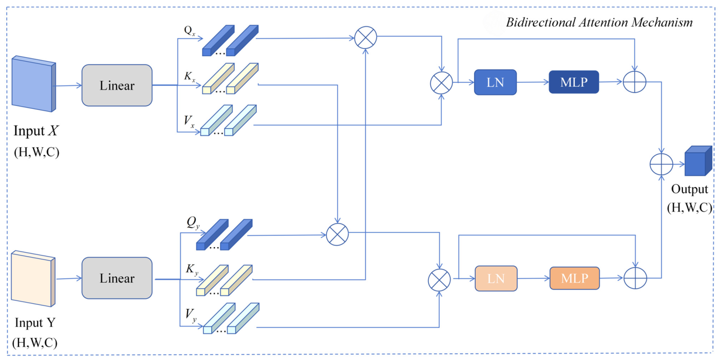
As shown in Figure 4, a window-based bidirectional cross-attention mechanism is employed to model the correlations between spectral components.

The dual-branch inputs are as follows:

$$X\in {ℝ}^{\mathrm{B}\times \mathrm{N}\times \mathrm{C}},\mathrm{N}={\mathrm{H}}_{\mathrm{x}}\times {\mathrm{W}}_{\mathrm{x}}.$$

(24)

$$Y\in {ℝ}^{\mathrm{B}\times \mathrm{M}\times \mathrm{C}},\mathrm{M}={\mathrm{H}}_{\mathrm{y}}\times {\mathrm{W}}_{\mathrm{y}}.$$

(25)

Here, B denotes the batch size, and ${\mathrm{H}}_{\mathrm{x}},{\mathrm{W}}_{\mathrm{x}}$ and ${\mathrm{H}}_{\mathrm{y}},{\mathrm{W}}_{\mathrm{y}}$ represent the numbers of windows along the height and width dimensions, respectively, forming nearly square regions. N and M denote the numbers of tokens in the X and Y branches.

In multi-head attention, the channel dimension satisfies $\mathrm{C}=\mathrm{h}\cdot \mathrm{d}$, where h is the number of heads and d is the dimension of each head, which is set to 8 in the experiments.

On the X branch:

$$Q_{\mathrm{X}}=X{W}_{\mathrm{Q}}\in {ℝ}^{\mathrm{B}\times \mathrm{N}\times \mathrm{d}},K_{\mathrm{Y}}=Y{W}_{\mathrm{K}}\in {ℝ}^{\mathrm{B}\times \mathrm{M}\times \mathrm{d}},V_{\mathrm{X}}=X{W}_{\mathrm{V}}\in {ℝ}^{\mathrm{B}\times \mathrm{M}\times \mathrm{d}}$$

(26)

$$Q_{\mathrm{Y}}=Y{W}_{\mathrm{Q}}\in {ℝ}^{\mathrm{B}\times \mathrm{M}\times \mathrm{d}},K_{\mathrm{X}}=X{W}_{\mathrm{K}}\in {ℝ}^{\mathrm{B}\times \mathrm{N}\times \mathrm{d}},V_{\mathrm{Y}}=Y{W}_{\mathrm{V}}\in {ℝ}^{\mathrm{B}\times \mathrm{N}\times \mathrm{d}}$$

(27)

On the Y branch:

Here, $W_{\mathrm{Q}}$, $W_{\mathrm{K}}$, and $W_{\mathrm{V}}$ are learnable projection matrices. For the two feature vectors X and Y, after processing through the fusion attention module and similarity computation, the representation can be expressed as:

$$\mathrm{Atten}(Q,K,V)=V\left(\mathrm{softmax}\right({\displaystyle \frac{Q{K}^{\mathrm{T}}}{\sqrt{\mathrm{d}}}}\left)\right).$$

(28)

$$\tilde{X}=\mathrm{MLP}\left(\mathrm{LN}\right({\mathrm{Atten}}_{\mathrm{x}}(Q_{\mathrm{X}},K_{\mathrm{Y}},V_{\mathrm{X}})+X\left)\right)+({\mathrm{Atten}}_{\mathrm{x}}(Q_{\mathrm{X}},K_{\mathrm{Y}},V_{\mathrm{X}})+X).$$

(29)

$$\tilde{Y}=\mathrm{MLP}\left(\mathrm{LN}\right({\mathrm{Atten}}_{\mathrm{y}}(Q_{\mathrm{Y}},K_{\mathrm{X}},V_{\mathrm{Y}})+Y\left)\right)+({\mathrm{Atten}}_{\mathrm{y}}(Q_{\mathrm{Y}},K_{\mathrm{X}},V_{\mathrm{Y}})+Y).$$

(30)

In the bidirectional attention mechanism proposed in this paper, the features of two modalities, namely HSI and MSI, are first mapped into a unified embedding space to generate the corresponding Q, K, and V tensors, respectively. The two modalities interact via a weighting mechanism based on Q-K similarity matching and adaptively aggregate the V features of their own modalities, so as to construct cross-modal contextual representations and model long-range dependencies. Unlike decoupled or sequential conditional modeling strategies [58], the proposed framework performs synchronous bidirectional updates within the same attention layer and forms a closed-loop information flow in the shared embedding space. The synchronous bidirectional update means that HSI and MSI act simultaneously as query ends and contextual ends for cross-modal interaction in the same attention layer. The HSI branch aggregates spatial information from MSI to update its own features, while the MSI branch aggregates spectral response information from HSI for self-feature updating. Different from the traditional unidirectional cross-attention that only takes one modality as the query to update a single branch, the proposed method avoids asymmetric information flow directions, enabling symmetric coupling and complementary enhancement of the two modalities under the same feature state. The closed-loop information flow in the shared embedding space indicates that after unified dimension mapping, HSI and MSI serve as mutual query and queried ends in the unified embedding space, forming bidirectional closed interactive paths. Through information transmission between closed-loop cross-modalities, bidirectional complementation of spatial details and spectral response information is realized, which further improves the alignment degree and fusion consistency of spectral and spatial features. This mechanism completes bidirectional updates in parallel within a single layer, reduces directional bias caused by serial modeling, and strengthens the symmetry and stability of cross-modal coupling.

To reduce computational complexity, a window partition strategy is introduced. However, the windows are not independently modeled. The partitioning operation modifies only the attention computation scheme rather than the underlying feature structure. Cross-window dependencies are preserved through (1) multi-scale feature extraction and cross-branch alignment within a unified spatial grid, allowing each local window to access global contextual information; (2) topology-preserving window partitioning that maintains global feature continuity; and (3) residual connections that progressively propagate cross-window information across network layers. Consequently, the proposed design achieves local computational efficiency while maintaining global inter-window dependency modeling capability.

$$\mathrm{BD}=\mathrm{Concat}(\mathrm{BiDAttentio}{\mathrm{n}}_{2,4,8}),\mathrm{BD}\in {ℝ}^{\mathrm{B}\times \mathrm{C}\times \mathrm{H}\times \mathrm{W}}.$$

(31)

The outputs from different groups after bidirectional attention are concatenated along the channel dimension:

A 1 × 1 convolution is then applied to restore the original channel dimension:

$$X_1={\mathrm{Conv}}_{1\times 1}\left(\mathrm{BD}\right),X_1\in {ℝ}^{\mathrm{B}\times \mathrm{C}\times \mathrm{H}\times \mathrm{W}}.$$

(32)

3.2.5. Spectral Compression and Spatial Guidance Mechanism

For the multispectral input, $Y\in {ℝ}^{\mathrm{B}\times \mathrm{c}\times \mathrm{H}\times \mathrm{W}}$ and the wavelet-fused feature tensor $X_{\mathrm{wavelet}}\in {ℝ}^{\mathrm{B}\times \mathrm{C}\times \mathrm{H}\times \mathrm{W}}$, as defined previously, are first fed into the spectral compression and guidance module.

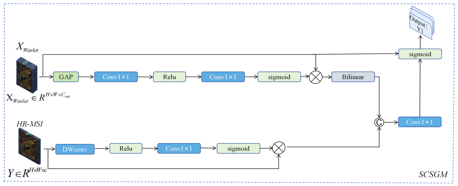
As shown in Figure 5, through global average pooling (GAP), the spatial responses of each spectral band are aggregated by averaging over the spatial dimensions, resulting in a compact global activation vector that captures channel-wise statistical information.

The formulation is given as follows:

$$X_{\mathrm{WG}}=\mathrm{GAP}(X_{\mathrm{wavelet}})={\displaystyle \frac{1}{\mathrm{HW}}}{\displaystyle \sum _{\mathrm{i}=1}^{\mathrm{H}}{\displaystyle \sum _{\mathrm{j}=1}^{\mathrm{W}}{X}_{\mathrm{wavelet}}^{(:,:,\mathrm{i},\mathrm{j})},X_{\mathrm{WG}}\in {ℝ}^{\mathrm{B}\times \mathrm{C}}}}.$$

(33)

Then, the output from the global feature extraction is passed through two 1 × 1 convolutional layers with two activation functions to generate the attention coefficients. The first convolution performs spectral compression, while the second restores the dimensionality and produces the attention coefficients. By incorporating residual connections, the module learns nonlinear mappings between different spectral bands.

The corresponding expression is given as follows:

$$A_{\mathrm{s}}=\mathsf{\sigma }(W_1\ast \delta (W_2\ast X_{\mathrm{WG}}\left)\right),W_1\in {ℝ}^{\mathrm{C}\times \mathrm{C}/\mathrm{r}\times 1\times 1},W_2\in {ℝ}^{\mathrm{C}/\mathrm{r}\times \mathrm{C}\times 1\times 1}.$$

(34)

where both ${\mathrm{W}}_1$ and ${\mathrm{W}}_2$ are convolutional layers and $\sigma (\cdot )$ denotes the Sigmoid activation function. Finally, bilinear upsampling is applied to restore the feature map to the same spatial size, yielding:

$$\widetilde{A_{\mathrm{s}}}=\mathrm{Upsampling}(A_{\mathrm{s}})$$

(35)

The following spatial guidance module mainly employs large-kernel depthwise convolutions. Through per-channel depthwise convolution and activation functions, the spatial weighting coefficients are obtained.

The specific formulation is as follows:

$$S_{\mathrm{m}}=\mathsf{\sigma }({\mathrm{Conv}}_{1\times 1}\left(\mathsf{\delta }\right(\mathrm{DWConv}(Y\left)\right)\left)\right).$$

(36)

Finally, through a joint gating mechanism, the channel attention map and the spatial guidance map are concatenated along the channel dimension.

The fused representation is then passed through a convolutional layer followed by an activation function to generate the final modulation coefficients.

$$Q=\mathrm{concat}(\widetilde{A_s},S_m),Q\in {ℝ}^{\mathrm{B}\times 2\mathrm{C}\times \mathrm{H}\times \mathrm{W}},$$

(37)

$$G=\mathsf{\sigma }(\mathrm{Con}{\mathrm{v}}_{1\times 1}(Q\left)\right),G\in {ℝ}^{\mathrm{B}\times \mathrm{C}\times \mathrm{H}\times \mathrm{W}}.$$

(38)

Finally, the output undergoes residual modulation. To avoid biased scaling caused by the Sigmoid activation, the attention map $G\in (0,1)$ is shifted by subtracting ${\displaystyle \frac{1}{2}}$, resulting in a zero-centered modulation range of (−0.5, 0.5). This allows both positive and negative feature adjustments, preventing excessive amplification and promoting balanced modulation.

The output is computed as:

$$Y_1=X_{\mathrm{wavlet}}\odot (1+\mathsf{\alpha }\cdot (\mathrm{G}-{\displaystyle \frac{1}{2}})),Y_1\in {ℝ}^{\mathrm{B}\times \mathrm{C}\times \mathrm{H}\times \mathrm{W}},\mathsf{\alpha }\in (0,1).$$

(39)

The scaling factor $\alpha$, initialized to 0.7, controls the modulation strength and preserves identity mapping when small, thereby ensuring stable feature propagation and improved convergence. Finally, the deeply extracted spectral feature $X_1$ and spatial feature $Y_1$ are fed into the BiDAttention module for another bidirectional attention operation. The output is residually fused with the intermediate wavelet features and restored to the original dimension via a convolutional layer, yielding the reconstructed HR-HSI.

The formulation is expressed as follows:

$$\widehat{Z}={\mathrm{Conv}}_{1\times 1}(\mathrm{Concat}(X_{\mathrm{Wavelet}},\mathrm{BiDAttention}(X_1,Y_1\left)\right]).$$

(40)

4. Experiments

To comprehensively evaluate the proposed framework, we conduct comparisons with twelve representative state-of-the-art fusion methods, including CNMF [5], CSU [13], SSE [20], MSDCNN [34], TFNet [35], ResTFNet [35], SFFCNN [14], RSST [56], SSR-NET [49], UMSFT [52], UPFW [50], and MCT-Net [55].

All experimental parameters are configured according to the original authors’ code or the recommendations provided in their papers. The traditional methods are tested using MATLAB R2014a on a system equipped with an Intel Core i9 processor and 32 GB RAM running Windows 11. The deep learning methods are implemented in Python 3.8 using PyTorch 1.8 and accelerated with an NVIDIA RTX 4060 Ti GPU. Data preprocessing and analysis are conducted using MATLAB R2014a, along with NumPy and Pandas libraries in Python.

The proposed network is implemented based on the PyTorch 2.8.0 framework and trained using the Adam optimizer with a learning rate of 1 × 10⁻⁴. During training, the mean squared error (MSE) loss is adopted to constrain the pixel-level differences between the reconstructed HSI and the reference HSI. Meanwhile, 128 × 128 spatial patches are randomly cropped from the training region as network inputs, with the batch size set to 4. The model is trained for 1000 epochs, and the checkpoint with the best validation PSNR is saved for final testing. To ensure the fairness and reliability of the evaluation, a central region with the same spatial size is selected as the test area and masked during training to avoid information leakage between the training and test samples.

4.1. Dataset Description

To verify the superiority of the proposed method, experiments were conducted on four publicly available datasets: Pavia University, Pavia Centre, Urban, and Washington DC Mall.

(1)

Pavia University:

The Pavia University dataset was also collected by the ROSIS sensor in 2003, with a spatial resolution of 1.3 m and an image size of 610 × 340 pixels. It initially contains 115 spectral bands; after discarding 12 noisy bands, 103 effective bands are used for further analysis.

(2)

Pavia Centre:

The Pavia Centre dataset was acquired in 2003 by the ROSIS sensor, covering the spectral range of 430–860 nm with a spatial resolution of 1096 × 715 pixels. The original data contain 115 spectral bands, of which 102 bands are retained after removing noisy and water absorption bands for subsequent processing.

(3)

Urban:

The Urban dataset was captured in 1995 by the HYDICE sensor over Copperas Cove, TX, USA. The dataset has a spatial size of 307 × 307 pixels and originally contains 210 spectral bands. After removing noisy and water absorption bands, 162 bands are retained for analysis.

(4)

Washington DC Mall (WDCM):

The WDCM dataset was collected in 1995 by the HYDICE sensor over the Washington DC Mall. It covers a wavelength range of 200–2400 nm and originally contains 210 spectral bands; after eliminating water vapor absorption bands, 191 bands are preserved. The spatial size of the image is 1280 × 307 pixels, with a spatial resolution of 2.5 m.

These datasets collectively cover diverse landscapes, including urban areas, vegetation, and natural ecosystems, providing a comprehensive evaluation of the proposed fusion framework’s robustness and adaptability.

4.2. Evaluation Metrics

To comprehensively evaluate the performance of the image fusion algorithm, multiple quantitative metrics are commonly used for comparison, including RMSE, PSNR, SAM, and ERGAS. These metrics are applied to verify the effectiveness of the proposed framework in the fusion task between LR-HSI and HR-MSI. The four metrics are described as follows:

(1)

Root Mean Squared Error (RMSE):

RMSE measures the error energy between the fused result and the ground truth (the square root of the mean squared error), directly reflecting the pixel-level intensity deviation.

$$\mathit{RMSE}=\sqrt{{\displaystyle \frac{1}{\mathit{HWC}}}{\displaystyle \sum _{c=1}^C{\displaystyle \sum _{i=1}^H{\displaystyle \sum _{j=1}^W{(R_k(i,j)-\widehat{R_k(i,j)})}^2}}}}.$$

(41)

Here, H, W, and C represent the height, width, and number of spectral bands of the image, respectively. A smaller value indicates better reconstruction quality.

(2)

Peak Signal-to-Noise Ratio (PSNR):

PSNR is one of the most widely used and objective image quality evaluation metrics. Essentially, it represents the capability of error suppression in terms of the signal-to-noise ratio.

$$\mathit{PSNR}=10{\mathit{log}}_{10}\left({\displaystyle \frac{L^2}{\frac{1}{\mathit{HW}}{\displaystyle \sum _{i,j=1}^{\mathit{HW}}{\left(R_k(i,j)-\widehat{R_k(i,j)}\right)}^2}}}\right)$$

(42)

Here, H and W denote the height and width of the image. A higher PSNR value indicates higher signal quality and better detail recovery.

(3)

Spectral Angle Mapper (SAM):

SAM measures the spectral angle between two spectral vectors, quantifying the similarity between spectral curves. It effectively evaluates spectral differences between remote sensing images.

$${\mathit{MSA}}_i={\displaystyle \frac{1}{\mathit{HW}}}{\displaystyle \sum _{i,j=1}^{\mathit{HW}}\mathit{arccos}\frac{<R_k(i,j),\widehat{R_k(i,j)}>}{\left|\right|R_i(i,j)|{|}_2\cdot \left|\right|\widehat{R_i}(i,j)|{|}_2}}$$

(43)

(4)

Error Relative Global Dimensionless Synthesis (ERGAS):

ERGAS essentially represents the normalized root mean square spectral error, which is used to quantify the relative variation of spectral errors across different bands and serves as a commonly used metric in multi-modal image fusion.

A lower ERGAS value indicates better fusion performance. Conversely, higher values mean poorer quality.

$$\mathit{ERGAS}=100\times {\displaystyle \frac{h}{l}}\sqrt{{\displaystyle \frac{1}{C}}{\displaystyle \sum _{c=1}^C{\left(\frac{\mathit{RMSE}(B_c)}{\overline{M_c}}\right)}^2}}$$

(44)

Here, h represents the resolution of HR-MSI, l denotes the resolution of LR-HSI, C is the number of spectral bands, $B_c$ is the radiance of HR-MSI, and $\overline{{\mathrm{M}}_{\mathrm{c}}}$ is the mean radiance of HR-MSI.

4.3. Experimental Implementation Details

In the spatial degradation process, a spatial degradation observation model combining Gaussian blurring and spatial downsampling is adopted to generate the LR-HSI. Specifically, the Gaussian filter is used to approximate the optical blurring effect caused by the sensor point spread function (PSF), while spatial downsampling is employed to simulate the spatial resolution loss resulting from the limited sampling capability of the sensor. This “blurring–downsampling” degradation model explicitly characterizes the optical blur and sampling degradation processes in practical imaging systems and has been widely used in hyperspectral–multispectral image fusion studies [68,69]. Following the experimental setting of Wei et al. [68], each spectral band of the reference HR-HSI is first convolved with a Gaussian low-pass filter with a kernel size of 5 and a standard deviation of $\mathsf{\sigma }=2$, and is then downsampled in both the horizontal and vertical directions with a scale factor of s = 4 to obtain the corresponding LR-HSI.

For spectral degradation, we adopt the official spectral response function (SRF) of the Sentinel-2 multispectral instrument (MSI) released by the European Space Agency (ESA) to perform spectral weighted integration on the reference high-resolution hyperspectral image (HR-HSI), thereby generating the high-resolution multispectral image (HR-MSI). This strategy introduces the band response characteristics of a real multispectral sensor, making the simulated spectral degradation process consistent with the physical imaging mechanism of the MSI sensor [69,70]. Specifically, the official Sentinel-2 SRF [71] document provides spectral response curves for 13 MSI bands. For each MSI band, its SRF is first resampled to the central wavelength positions of the hyperspectral bands. Then, the hyperspectral bands overlapping with the response range of the corresponding MSI band are weighted and integrated, and the response weights are normalized so that their sum equals 1. In this way, the spectral sensitivity characteristics of each MSI band can be preserved. As shown in

Table 2. Dataset spectral ranges and Sentinel-2 MSI band selection for spectral degradation simulation.

Dataset	Spectral Range	Sentinel-2 Bands Used	Number of MSI Bands
Pavia	430–860 nm	B1–B8	8
PaviaU	430–860 nm	B1–B8	8
Urban	400–2400 nm	B1–B8, B8a, B9, B11, B12	12
Washington	400–2400 nm	B1–B8, B8a, B9, B11, B12	12

, since different hyperspectral datasets have different valid wavelength ranges, only the Sentinel-2 bands overlapping with the wavelength range of each dataset are selected for simulation. Specifically, the Pavia and PaviaU datasets use B1–B8, resulting in eight simulated multispectral bands, while the Urban and Washington datasets use B1–B8, B8a, B11, and B12, resulting in twelve simulated multispectral bands.

The spectral degradation process can be formulated as:

$$M_b(x,y)={\displaystyle \frac{{\displaystyle {\sum }_{i\in {\Omega }_b}{R}_b\left({\mathsf{\lambda }}_i\right)H(x,y,{\mathsf{\lambda }}_i)}}{{\displaystyle {\sum }_{i\in {\Omega }_b}{R}_b\left({\mathsf{\lambda }}_i\right)}}}$$

(45)

where ${\mathrm{M}}_{\mathrm{b}}(\mathrm{x},\mathrm{y})$ denotes the simulated value of the b-th MSI band at spatial position (x, y), $\mathrm{H}(\mathrm{x},\mathrm{y},{\mathsf{\lambda }}_i)$ denotes the HR-HSI value at wavelength ${\mathsf{\lambda }}_i$, ${\mathrm{R}}_{\mathrm{b}}\left({\mathsf{\lambda }}_{\mathrm{i}}\right)$ represents the spectral response value of the b-th Sentinel-2 MSI band at ${\mathsf{\lambda }}_i$, and ${\Omega }_b$ denotes the set of hyperspectral bands overlapping with the response range of the b-th MSI band.

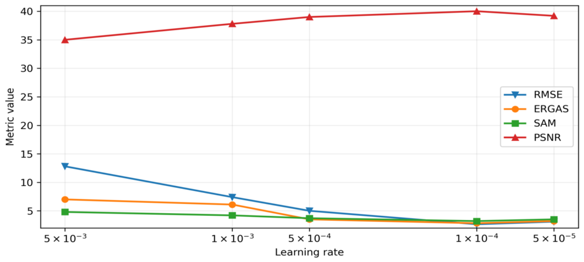
In Figure 6, we evaluated the fusion performance under different learning rates on the Pavia Center dataset and ultimately determined to adopt a learning rate of 0.0001 based on the experimental data.

4.4. Comparison with Existing Popular Methods

We compare our proposed method with twelve mainstream hyperspectral image fusion algorithms across multiple datasets.

These methods include CNMF [5], CSU [13], SSE [20], MSDCNN [34], TFNet [35], ResTFNet [35], SFFCNN [14], RSST [56], SSR-NET [49], UMSFT [52], UPFW [50], and MCT-Net [55].

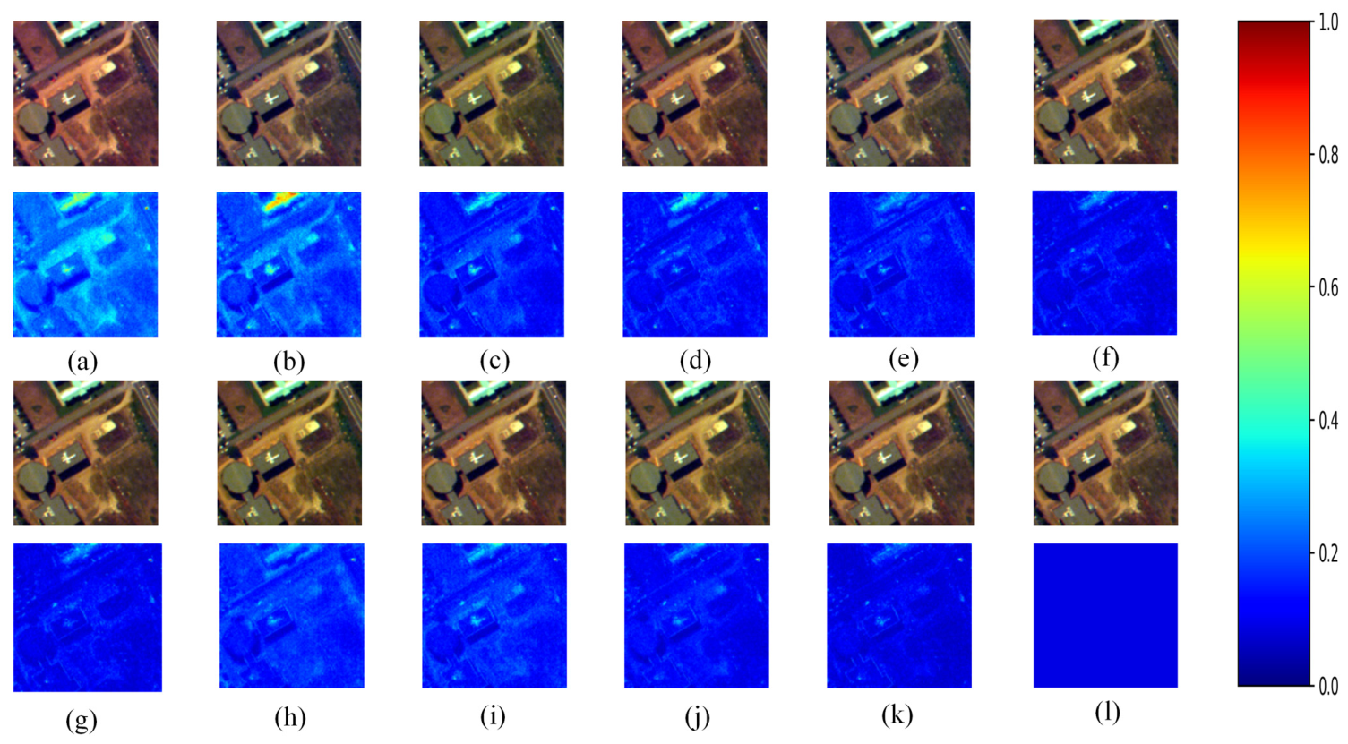
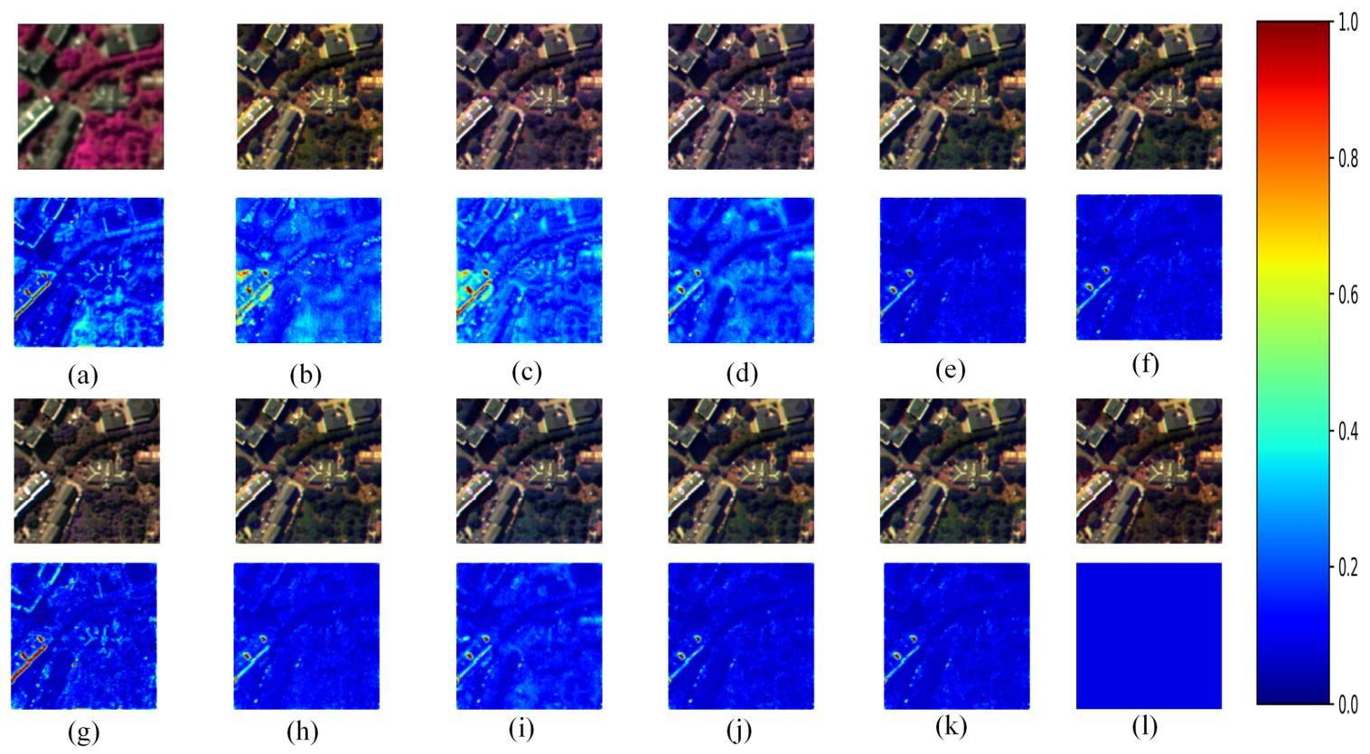
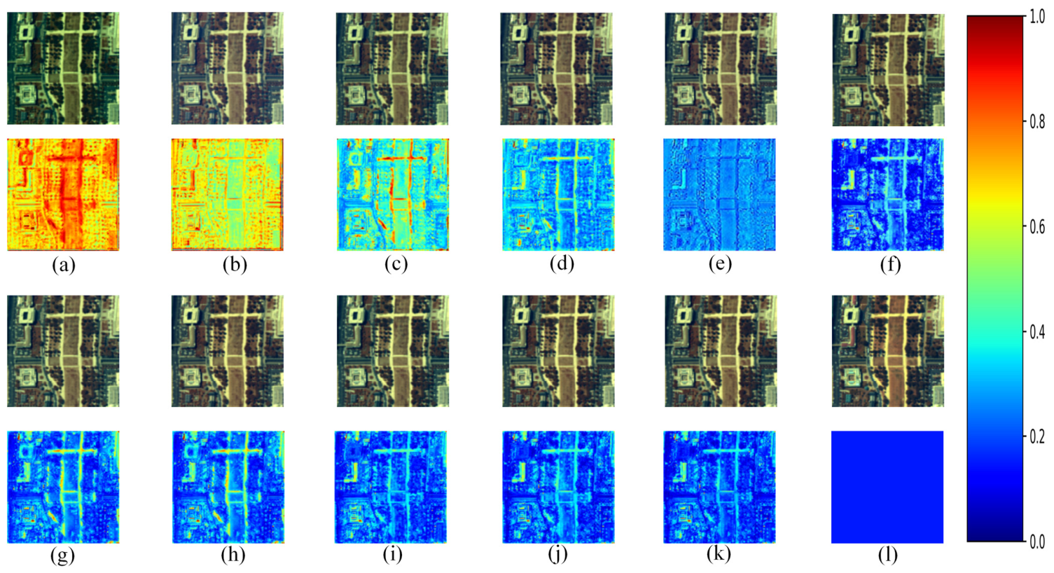
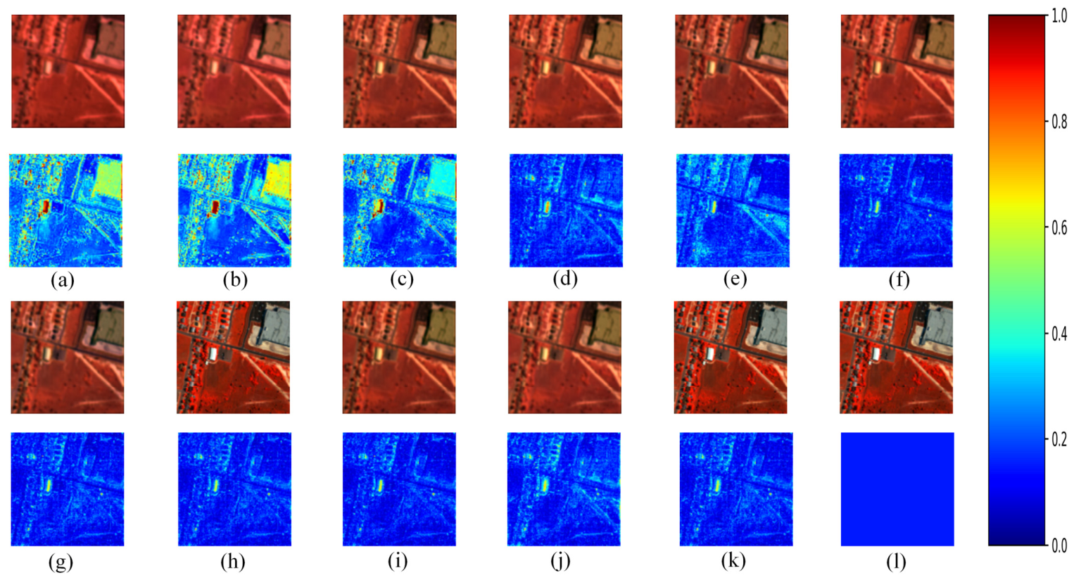
For visualization, pseudo-RGB images are generated by selecting three representative spectral bands. To ensure fair comparison, a shared linear stretching strategy is adopted within each dataset, where the stretching parameters are computed from the ground truth (GT) using percentile normalization and consistently applied to all methods. Considering that different datasets exhibit distinct dynamic ranges, the color scales are independently normalized per dataset rather than using a global scale. For residual visualization, the mean absolute error across spectral bands is normalized into [0, 1] using a hybrid scheme that combines percentile clipping and GT-based scaling, resulting in relatively scaled and visually stable error maps.

To comprehensively evaluate the robustness of the proposed method, all methods are compared under two spatial downsampling scales (4× and 8×). The quantitative results are reported under both degradation scales, while the visual results are presented under the 4× downsampling setting.

(1)

Results on the Pavia University Dataset

As shown in

Table 3. Comparison results on the Pavia University dataset under 4× and 8× downsampling settings. The best and second-best results under 4× are highlighted in red and blue, respectively, while those under 8× are marked in bold and underlined, respectively.

Method	Ratio	RMSE	PSNR	ERGAS	SAM
CNMF [5]	4×	5.7876	32.3376	3.2392	2.9969
	8×	6.2612	31.4217	4.0123	3.8641
CSU [13]	4×	2.8756	38.5978	2.9939	2.8227
	8×	3.0152	37.6817	3.0112	2.9001
SSE [20]	4×	2.4140	40.6732	2.6333	2.5614
	8×	2.5121	40.4318	2.8416	2.6124
MSDCNN [34]	4×	2.4313	40.7122	2.6358	2.6326
	8×	2.4891	40.6486	2.6051	2.6211
TFNet [35]	4×	2.2317	40.9234	2.1211	2.2891
	8×	2.2471	40.9115	2.1305	2.2954
ResTFNet [35]	4×	2.1578	41.7567	1.4968	2.1117
	8×	2.1541	41.7496	1.5000	2.1247
SSFCNN [14]	4×	1.9513	42.1234	1.3457	2.1781
	8×	1.9674	42.2153	1.3758	2.1741
RSST [56]	4×	1.5793	43.8466	1.2711	1.9099
	8×	1.5413	43.9423	1.2415	1.8673
SSR-NET [49]	4×	1.6447	43.4938	1.2646	2.0019
	8×	1.6443	43.5007	1.2481	1.9989
UMSFT [52]	4×	1.6779	43.0089	1.2699	2.2301
	8×	1.6841	43.0014	1.2745	2.2316
UPFW [50]	4×	1.9335	42.8697	2.1349	2.7101
	8×	1.9329	42.8864	2.1299	2.6546
MCT-NET [55]	4×	1.5455	43.9284	1.2527	1.8624
	8×	1.5511	43.9064	1.2484	1.8705
AWD-Net (Ours)	4×	1.3974	44.8662	1.1016	1.6989
	8×	1.3989	44.8009	1.1947	1.7345

, which presents the evaluation metrics for the Pavia University dataset, it is evident that our fusion method achieves significant improvements compared to both the traditional CNMF method and the deep learning-based RSST method.

Figure 7 presents the pseudo-color processed difference images of various methods, and it can be clearly observed that darker blue shades indicate better fusion performance. Our method adopts a synchronous bidirectional coupling update of cross-modal features. Compared with MCT-NET, which relies on traditional unidirectional and cascaded information transmission, it achieves simultaneous updates. A visual inspection clearly demonstrates that our network framework achieves optimal fusion results.

Since the PaviaU dataset contains a wide variety of urban land-cover types, the spectral responses among different classes vary significantly, and complex mixed pixels exist in local regions. RSST shows strong residual responses when recovering transition areas between roads and buildings, while the proposed method better preserves fine-grained details along boundaries such as rooftops and road edges.

It can be observed that RSST exhibits strong robustness under a higher degradation scale and still maintains competitive fusion performance under the 8× downsampling setting. In comparison, our proposed method shows a slight performance decrease under 8× downsampling compared with the 4× setting, but it still achieves the better results on the main evaluation metrics. This indicates that the proposed framework maintains good stability and adaptability even under more severe spatial degradation conditions.

(2)

Results on the Pavia Centre Dataset

Visual comparison clearly demonstrates that our fusion framework achieves superior performance. As shown by the quantitative metrics in

Table 4. Comparison results on the Pavia Centre dataset under 4× and 8× downsampling settings. The best and second-best results under 4× are highlighted in red and blue, respectively, while those under 8× are marked in bold and underlined, respectively.

Method	Ratio	RMSE	PSNR	ERGAS	SAM
CNMF [5]	4×	11.9656	24.7872	10.7628	4.1572
	8×	13.5614	22.4816	11.6849	5.0217
CSU [13]	4×	5.1234	35.4278	5.9126	5.6245
	8×	6.1548	34.0749	6.4769	6.0492
SSE [20]	4×	4.0115	37.3271	4.3480	4.6781
	8×	4.1259	37.1594	4.4574	4.7564
MSDCNN [34]	4×	4.2341	34.9687	4.2999	5.3973
	8×	4.2864	34.8744	4.3094	5.4561
TFNet [35]	4×	4.1678	36.6389	4.5343	4.6827
	8×	4.1744	36.5996	4.5684	4.6994
ResTFNet [35]	4×	3.8845	37.4512	4.1591	4.4459
	8×	3.9023	37.4308	4.1620	4.4867
SSFCNN [14]	4×	4.8011	34.4192	5.6190	5.6893
	8×	4.7999	34.4203	5.6075	5.6412
RSST [56]	4×	2.9641	39.1121	3.1249	3.7045
	8×	2.9645	39.1241	3.1154	3.6347
SSR-NET [49]	4×	3.9158	37.8190	3.6961	3.5642
	8×	3.8541	38.0454	3.5841	3.4648
UMSFT [52]	4×	3.8864	38.8973	3.4684	3.7807
	8×	3.8854	38.8985	3.4671	3.7745
UPFW [50]	4×	3.8989	37.9871	3.8815	3.8475
	8×	3.7456	38.1873	3.6814	3.7846
MCT-NET [55]	4×	2.8225	39.4783	3.0519	3.5574
	8×	2.7365	39.5472	2.9844	3.3479
AWD-Net (Ours)	4×	2.6447	40.0194	2.8271	3.1997
	8×	2.6510	39.8947	2.9434	3.2546

, our method consistently outperforms all competing approaches across all four evaluation indicators. Specifically, compared to the second-best method MCT-NET, it achieves a 10.06% reduction in the SAM metric. These results fully validate that the pixel-wise adaptive wavelet extraction architecture, when combined with subsequent deep feature extraction modules, effectively establishes long-range information dependencies while preserving excellent spectral fidelity and spatial resolution.

As shown in the visualization results of Figure 8, the reconstruction errors of different methods are mainly concentrated in transition regions, such as building boundaries and road intersections. The traditional CNMF method struggles to accurately recover boundary details and tends to produce blurring and spectral distortion around edge regions. In contrast, deep learning-based methods, such as MCT-Net and the proposed method, exhibit lower errors around building contours and road edges, indicating that they can achieve a better balance between spatial detail preservation and spectral consistency.

(3)

Results on the Urban Dataset

The experimental results on the Urban dataset are presented in

Table 5. Comparison results on the Urban dataset under 4× and 8× downsampling settings. The best and second-best results under 4× are highlighted in red and blue, respectively, while those under 8× are marked in bold and underlined, respectively.

Method	Ratio	RMSE	PSNR	ERGAS	SAM
CNMF [5]	4×	3.9781	35.4867	1.9789	2.8869
	8×	4.3541	34.1571	2.2418	3.0014
CSU [13]	4×	2.8675	36.9924	1.4844	2.5727
	8×	3.0145	35.9994	1.9946	2.6871
SSE [20]	4×	2.8152	37.1365	1.4477	2.3955
	8×	3.0018	36.0049	1.9007	2.5047
MSDCNN [34]	4×	3.0377	36.0006	1.9013	2.5191
	8×	3.0541	35.9987	1.9954	2.6945
TFNet [35]	4×	3.0104	36.5234	1.8461	2.6254
	8×	3.0015	36.4924	1.8649	2.6007
ResTFNet [35]	4×	2.7861	36.5649	1.7807	2.6535
	8×	2.8454	36.3534	1.8741	2.6662
SSFCNN [14]	4×	5.7188	29.8335	3.0896	5.6141
	8×	5.6954	30.1248	2.9429	4.9542
RSST [56]	4×	2.5861	37.9815	1.3569	2.3416
	8×	2.5841	37.9844	3.3512	2.3048
SSR-NET [49]	4×	2.2330	38.5655	1.2133	2.2124
	8×	2.2274	38.6541	1.2004	2.1989
UMSFT [52]	4×	2.4551	38.1152	1.2542	2.2211
	8×	2.5234	38.0046	1.3514	2.3058
UPFW [50]	4×	2.5184	37.9987	1.3145	2.3011
	8×	2.5164	37.9999	1.3104	2.2994
MCT-NET [55]	4×	2.4763	37.7574	1.3348	2.2271
	8×	2.4786	37.7492	1.3350	2.2341
AWD-Net (Ours)	4×	1.9983	40.0021	1.0298	1.8864
	8×	1.9945	40.0947	1.0177	1.8465

and Figure 9. Through comparative analysis, it is evident that our fusion strategy achieves a significant 3.73% improvement in PSNR and a 14.74% reduction in the SAM metric compared to the suboptimal fusion approach. In contrast to SSR-NET, which adopts spatial–spectral concatenated recovery combined with edge loss constraints and thus has limited representation capability, the proposed method employs a deep cross-interaction dynamic information flow that enables bidirectional synchronous coupling.

The Urban dataset contains more complex urban spatial structures, where SSR-Net shows relatively clear advantages. This is mainly because its spatial–spectral residual network explicitly constrains the image fusion process by jointly using spatial edge loss and spectral edge loss, thereby enhancing local structural representation while preserving the overall spectral trend. In addition, the bidirectional attention mechanism and grouped convolution adopted in the proposed method can capture fine-grained band differences at different spectral scales, enabling it to achieve superior performance in such complex urban scenes.

(4)

Results on the Washington DC Mall Dataset

The Washington DC Mall dataset contains a large number of spectral bands and has high spatial resolution. However, our method still achieves significant improvements in both the spectral and spatial dimensions. The effect is clearly visible in Figure 10.

As shown in

Table 6. Comparison results on the Washington DC Mall dataset under 4× and 8× downsampling settings. The best and second-best results under 4× are highlighted in red and blue, respectively, while those under 8× are marked in bold and underlined, respectively.

Method	Ratio	RMSE	PSNR	ERGAS	SAM
CNMF [5]	4×	30.1541	16.7894	13.2909	21.4689
	8×	31.0246	16.1468	14.0458	22.3547
CSU [13]	4×	2.3683	44.5656	0.3952	0.3941
	8×	2.6484	43.7484	0.5417	0.4573
SSE [20]	4×	2.3152	44.8589	0.3447	0.4274
	8×	2.4782	43.5746	0.4456	0.4575
MSDCNN [34]	4×	2.7182	40.0435	0.3687	0.6939
	8×	2.7214	40.1054	0.3811	0.6843
TFNet [35]	4×	2.8094	39.7566	0.4001	0.7464
	8×	2.8001	39.7843	0.3993	0.7541
ResTFNet [35]	4×	2.6438	41.6816	0.3153	0.6861
	8×	2.6541	41.6984	0.3101	0.6783
SSFCNN [14]	4×	16.6101	22.7311	3.1689	6.6787
	8×	15.2484	24.2548	2.9584	5.3215
RSST [56]	4×	1.3684	43.9461	1.5618	0.4976
	8×	1.3666	43.9561	1.5240	0.4894
SSR-NET [49]	4×	2.1911	40.0087	0.3315	0.6891
	8×	2.0156	40.9456	0.2874	0.5783
UMSFT [52]	4×	1.5124	43.4552	0.5631	0.5113
	8×	1.5014	43.5416	0.5348	0.5000
UPFW [50]	4×	1.9882	42.7077	1.4809	2.3648
	8×	1.9456	42.9453	1.4652	2.2415
MCT-NET [55]	4×	1.2683	44.8781	0.1812	0.4123
	8×	1.2771	44.7538	0.1943	0.4359
AWD-Net (Ours)	4×	1.0074	45.6985	0.1622	0.3291
	8×	1.0159	45.6643	0.1735	0.3948

, compared with the advanced MCT-Net model, our method achieves a 1.83% improvement in PSNR and reduces RMSE by approximately 20.57%. These results indicate that AWD-Net is particularly effective in modeling high-dimensional spectral correlations while preserving fine-grained spatial details. This can be attributed to its unified cross-modal interaction design, which facilitates efficient information exchange and joint optimization across spatial and spectral domains, even under complex data distributions.

The proposed method maintains a low overall error in large homogeneous regions, while also showing good structural preservation in areas where fusion errors tend to concentrate, such as water boundaries and transition regions between vegetation and artificial objects. Compared with other methods, our proposed method exhibits a smoother error distribution in complex boundary regions. This indicates that it can not only recover the global spectral trend but also effectively constrain local spatial details, thereby achieving more stable fusion performance in large-scale complex scenes.

4.5. Ablation Study

To evaluate the impact of each module in the AWD-Net framework on the fusion performance, we conducted ablation experiments on the individual components of AWD-Net.

4.5.1. Ablation on the Adaptive Wavelet Transform

This module dynamically selects the most appropriate subband responses in the wavelet domain, enabling adaptive feature extraction for various regions, including textures, edges, and smooth areas. Within the overall framework, this module is embedded before the spatial–spectral dual-branch structure, allowing the input low-resolution hyperspectral (LR-HSI) and high-resolution multispectral (HR-MSI) data to obtain frequency-domain enhanced features at the early fusion stage.

To verify the effectiveness of this module, we conducted a systematic ablation study: keeping all other parts of the network identical, we compared different training strategies for the adaptive wavelet transform module. Specifically, the input LR-MSI has a size of 128 × 128, and the LR-HSI has a size of 32 × 32. We compared one-iteration and three-iteration training strategies and analyzed how weight sharing between iterative blocks affects performance.

When weights are shared across iterations, the model has fewer parameters and is computationally more efficient. When weights are not shared, each iteration can learn independent feature representations, thereby enhancing the model’s multi-stage fitting capability.

To assess these training strategies, experiments were conducted on the Pavia University dataset, recording four evaluation metrics (RMSE, PSNR, ERGAS, and SAM).

As shown in

Table 7. Ablation experimental results of the adaptive wavelet transform on the Pavia University Dataset. The best and second-best results are highlighted in red and blue.

Method	RMSE	PSNR	ERGAS	SAM
AWTM (1 iteration, shared weights)	1.3974	44.8662	1.1016	1.6989
AWTM (3 iterations, shared weights)	1.6530	44.0641	1.1798	1.6743
AWTM (1 iteration, unshared weights)	1.3974	44.8662	1.1016	1.6989
AWTM (3 iterations, unshared weights)	1.3412	44.9974	1.0787	1.6658

, the proposed pixel-wise adaptive wavelet transform model (AWTM) achieves excellent performance across all four evaluation metrics. In the iterative architecture, the SR-HSI obtained from the first round of adaptive wavelet reconstruction is regarded as the updated hyperspectral prior. After re-encoding through shallow convolution, it serves as the input for the next iteration, undergoing adaptive wavelet decomposition and gated fusion again with the same MSI image. This enables the model to reselect optimal wavelet bases based on the current error distribution. Residual information is generated through inverse transformation, thereby progressively correcting spectral distortion and complementing spatial details. This cyclic process of “previous output → adaptive wavelet decomposition → weighted reconstruction → residual update” endows the model with capabilities analogous to iterative optimization.

The comparison results between weight sharing and non-sharing indicate that assigning independent parameters to each iteration can significantly enhance the model’s stage-wise representation capacity, allowing different iterations to focus on repairing features at varying scales. This approach ultimately improves the Peak Signal-to-Noise Ratio (PSNR) by approximately 0.131 dB, while also achieving significant reductions in both Root Mean Square Error (RMSE) and Relative Global Error in Synthesis (ERGAS). Conversely, increasing the number of iterations in the weight-sharing configuration did not yield performance gains, indicating that repeated application of the same operator leads to representational redundancy and gradient coupling, thereby hindering the model’s ability to learn new details.

Considering both performance and model complexity, we ultimately adopted the single-iteration, non-shared weight wavelet transform module as the standard configuration, achieving strong generalization capability while maintaining a low parameter count.

To further verify the necessity of the adaptive wavelet selection mechanism, we conducted an additional comparison between six fixed wavelet bases and the proposed adaptive wavelet transform module. In this experiment, the subsequent spatial–spectral dual-branch structure was removed, so that the analysis focuses only on the contribution of the adaptive wavelet transform module, while the remaining network structure and training settings were kept consistent. As shown in

Table 8. Ablation study on the necessity of adaptive wavelet selection on the Pavia Centre dataset. The best and second-best results are highlighted in red and blue.

Method	RMSE	PSNR	ERGAS	SAM
Fixed-db4	3.3240	37.6975	3.8093	3.5495
Fixed-db6	3.5056	37.2353	3.9952	3.8931
Fixed-sym6	3.4568	37.3572	3.9438	3.8125
Fixed-coif5	3.5438	37.1413	4.0447	3.8475
Fixed-bior53	3.5493	37.1277	4.0187	3.9182
Fixed-Bior97	3.5080	37.2294	3.9894	3.8110
Only-AWTM	2.9164	38.6529	3.4216	3.4741

, changing only the wavelet basis leads to noticeable performance variations. Among the fixed wavelet bases, db4 achieves the best performance. In contrast, the RMSE values of coif5 and bior53 increase to 3.5438 and 3.5493, respectively, while their PSNR values decrease to 37.1413 and 37.1277. These results indicate that the choice of wavelet basis directly affects the model’s ability to recover spatial details and preserve spectral information, and that a single fixed wavelet basis is easily limited by its inherent decomposition characteristics. Compared with db4, our AWTM achieves the best performance among the fixed wavelet bases, and our method outperforms it on all four evaluation metrics. Specifically, RMSE is reduced by approximately 12.26%, and ERGAS is reduced by approximately 10.18%. This demonstrates that the advantage of the proposed method does not simply come from relying on a specific wavelet basis, but from dynamically adjusting the contributions of different wavelet bases through the gating mechanism. In this way, the model can better exploit the complementary representation abilities of multiple wavelet bases for edge details, texture structures, and smooth regions, confirming the necessity of the adaptive wavelet selection mechanism.

To further analyze the spatial–spectral representation differences among different wavelet bases, it can be observed that db4 and db6, although both belonging to the Daubechies wavelet family, show clear performance differences. db4 achieves the best performance among the fixed wavelet bases, whereas db6 increases the RMSE to 3.5056 and decreases the PSNR to 37.2353. This result suggests that, for the Pavia Centre dataset, increasing the wavelet order does not necessarily lead to better fusion performance. The Pavia dataset contains complex land-cover regions, requiring both the recovery of high-frequency spatial details and the preservation of spectral continuity in smooth regions. Compared with db6, db4 has a relatively shorter support range and is more sensitive to local discontinuities and fine structural variations, making it more suitable for preserving edge contours and local textures in urban scenes. In contrast, although the wider support range of db6 may be beneficial for smooth representation, it may reduce sensitivity to fine edges and local textures. Similarly, the different results of sym6, coif5, and the bior wavelets indicate that different wavelet bases have different adaptability to various land-cover regions in the Pavia Centre dataset. Therefore, relying on a single fixed wavelet basis makes it difficult to simultaneously preserve structural details and spectral consistency in complex urban hyperspectral images.

4.5.2. Ablation on the MSGC

To validate the effectiveness of multi-scale grouped convolution and the bidirectional attention mechanism, in the experiments, we used the upsampled LR-HSI and the original MSI as input branches, retaining one round of non-shared adaptive wavelet modules and spatial extraction modules. Under the same training conditions, the impact of different grouping and scale configurations on the experimental results was compared.

As shown in

Table 9. Ablation results of the GSGC of Group on the Pavia University Dataset. The best and second-best results are highlighted in red and blue.

Method	RMSE	PSNR	ERGAS	SAM
Group: 1, 3, 9	1.5641	43.8465	1.2611	1.8741
Group: 2, 4, 8	1.3974	44.8662	1.1016	1.6989
Group: 4, 8	1.6495	43.4562	1.2712	1.9684
Group: 2	1.7546	43.1456	1.3150	2.0012

, in the grouping experiments, the configurations were set as three groups: 1, 3, 9; 2, 4, 8; two groups: 4, 8; and one group: 2. The scale configurations were maintained as 3 × 3, 5 × 5, and 7 × 7, as in the paper. This experiment aimed to verify whether different grouping strategies would affect the experimental results.

Based on the above data, it can be observed that the grouping strategy of 2, 4, and 8 adopted in this study achieves better accuracy. Hyperspectral images exhibit strong local continuity along the spectral dimension, where adjacent bands are highly correlated, while the degree of information redundancy and spectral variation differs across different band ranges. Therefore, a single grouping scale is insufficient to simultaneously capture the global spectral trend and local spectral differences. According to the experimental results, single-group or few-group settings show relatively limited performance, whereas group = 4 and group = 8 outperform group = 2, indicating that medium- and fine-grained grouping strategies are more effective in enhancing local spectral feature representation. Furthermore, the combination of group = 2, 4, and 8 achieves the best performance, suggesting that coarse-, medium-, and fine-grained spectral partitioning are complementary. Specifically, coarse-grained grouping helps preserve the overall spectral structure, medium-grained grouping captures spectral variations within a moderate range, and fine-grained grouping is more suitable for modeling local band differences. By combining these three grouping scales, the model can obtain both global spectral context and local spectral details, thereby improving fusion performance. In contrast, the performance of group = 1, 3, and 9 is inferior to that of group = 2, 4, and 8, indicating that the grouping strategy is not effective when arbitrarily selected. The grouping scales of 2, 4, and 8 follow a binary hierarchical partitioning manner, forming a stable coarse-to-fine spectral modeling process. In comparison, irregular group settings, such as 1, 3, and 9, may lead to imbalanced band numbers and weakened spectral correlations within each subgroup, thereby reducing the ability to preserve the continuity of adjacent spectral bands.

4.5.3. Ablation on the Bidirectional Cross-Attention

Therefore, while keeping the grouping unchanged, we aim to verify whether the bidirectional attention mechanism truly achieves cross-scale attention correlation. In the ablation experiment, all bidirectional attention modules are replaced with the self-attention mechanism from Transformer. Additionally, with the self-attention mechanism adopted, bidirectional attention interaction between ${\mathbf{X}}_{\mathbf{1}}$ and ${\mathbf{Y}}_{\mathbf{1}}$ is not performed at the final stage; instead, they are concatenated along the channel dimension and then convolved back to the original dimensions. The final experimental results are shown in

Table 10. Ablation results of the Attention mechanism on the Pavia University Dataset. The best and second-best results are highlighted in red and blue.

Method	RMSE	PSNR	ERGAS	SAM
Self-Attention	1.8736	42.9412	2.1123	2.2264
Bidirectional Cross-Attention	1.3974	44.8662	1.1016	1.6989
Ca Attention	1.7561	43.1254	1.3789	2.0126
Dual cross-attention transformer	1.7546	43.8592	1.2964	1.9236

.

It can be observed that after switching to the self-attention mechanism, all evaluation metrics underperform compared to the bidirectional attention. The PSNR metric decreased by 2.24%, while the SAM metric surged by 13.63%. This indicates that the bidirectional cross-scale attention mechanism can effectively capture the spatial and spectral relationships between the original hyperspectral data and the fused data. To a large extent, it compensates for the detail loss and other feature deficiencies caused by convolution, thereby achieving efficient performance.

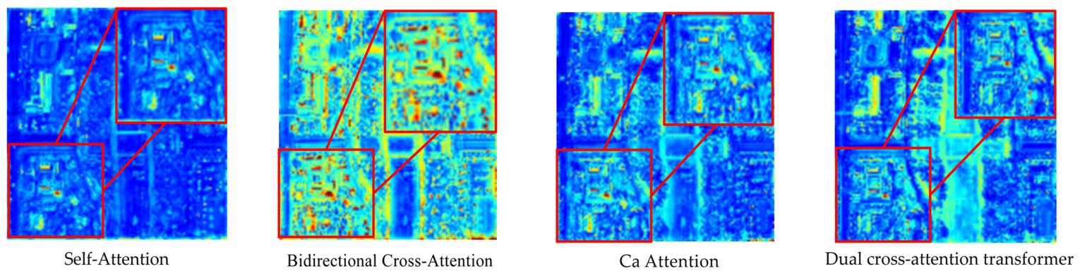
In addition, this study compares the proposed method with the state-of-the-art Dual Cross-Attention Transformer [58] and Ca Attention [57]. To ensure a fair comparison, the analysis focuses primarily on differences at the attention-mechanism level rather than on overall network architecture design. Specifically, under the same backbone structure, only the attention modules are replaced, enabling a more direct evaluation of the modeling capabilities of different cross-modal interaction strategies.

As shown in Figure 11, this paper visualizes the attention mechanism on the highly challenging Washington DC Mall dataset. In the attention heatmap, warmer colors indicate stronger responses of the attention mechanism. It is worth noting that although a similar color scheme is used as in the fused pseudo-color visualization results mentioned above, their physical meanings are exactly opposite.

The experimental results demonstrate that the proposed bidirectional attention mechanism achieves clear performance advantages. One reason is that the Dual Cross-Attention Transformer can essentially be regarded as a combination of two unidirectional cross-attention modules, where each direction is modeled separately. Although this design enables bidirectional information flow, the interaction process remains relatively decoupled. Ca Attention, in contrast, mainly enhances single-feature representations through intra-domain recalibration in the spatial and spectral domains. It emphasizes internal dependency modeling but does not explicitly construct cross-modal correspondences between hyperspectral and multispectral data.

However, the key to hyperspectral–multispectral fusion lies in cross-modal joint modeling and complementary information alignment, rather than merely intra-domain feature enhancement. In comparison, the proposed method performs bidirectional cross-attention within the same layer, enabling synchronous updating and coupled interaction between the two modalities. This design strengthens symmetric constraints and complementary modeling capability, making it more suitable for fusion tasks involving strong complementarity between hyperspectral and multispectral images.

4.5.4. Ablation on the SCSGM

Finally, to further validate the impact of deep learning modules in the network on fusion performance, we extracted and independently tested the model with only the Spectral Compression and Spatial Guidance Module. This module uses depthwise separable convolutions and a feature attention mechanism. It precisely captures the interactive relationships between spatial textures and spectral information.

As shown in

Table 11. Ablation results of the SCSGM of Group on the Pavia University Dataset. The best results are highlighted in red.

Method	RMSE	PSNR	ERGAS	SAM
Without SCSGM	1.6064	43.7542	1.3429	1.9587
With SCSGM	1.3974	44.8662	1.1016	1.6989

, the SCSGM effectively learns spectral feature differences between spatial regions and achieves strong guidance among spatial features. The PSNR increased by 1.1120 dB, and the SAM decreased by 0.2598 dB. These results confirm that this module makes a significant contribution to noise suppression and spectral consistency.

In summary, the multi-level ablation studies clearly demonstrate the role and necessity of each sub-module in the overall architecture. Specifically, the pixel-level adaptive wavelet selection module is responsible for frequency domain enhancement and noise suppression, the multi-scale grouped convolution module enables fine-grained spectral feature extraction, and the spatial–spectral guidance module provides structural constraints and cross-dimensional feature reconstruction. The organic integration of these three components significantly enhances the comprehensive performance of hyperspectral and multispectral image fusion, providing a robust technical foundation for high-fidelity reconstruction of complex remote sensing imagery.

4.5.5. Time Efficiency Analysis of the Model

As shown in

Table 12. FLOPs and parameters of the proposed AWD-Net and other deep learning models on the Pavia University dataset.

Method	Params (M)	FLOPs (G)	PSNR	SAM
MSDCNN	2.10	34.47	40.7122	2.6326
TFNet	2.53	10.37	40.9234	2.2891
ResTFNet	2.40	9.72	41.7567	2.1117
SSFCNN	0.66	10.76	42.1234	2.1781
RSST	2.91	47.34	43.8466	1.9099
SSR-Net	1.64	33.45	43.4938	2.2319
MCT-Net	11.23	43.50	43.9284	1.8624
AWD-Net (ours)	1.82	32.01	44.8662	1.6989

, AWD-Net contains only 1.82 M parameters, which is significantly lower than MCT-Net with 11.23 M parameters, and also lower than MSDCNN, TFNet, ResTFNet, and RSST. This indicates that the proposed model maintains a relatively compact parameter scale. In terms of computational complexity, AWD-Net requires 32.01 G FLOPs, which is lower than MSDCNN, SSR-Net, RSST, and MCT-Net, but higher than SSFCNN, TFNet, and ResTFNet. This is mainly because AWD-Net introduces the adaptive wavelet transform, grouped multi-scale convolution, and spatial–spectral feature interaction modules, which bring additional computational cost. Although AWD-Net does not achieve the lowest FLOPs, it obtains the highest PSNR and the lowest SAM, demonstrating that it can effectively improve spatial detail recovery and spectral consistency preservation with a relatively small number of parameters, achieving a favorable balance between model complexity and fusion performance.

5. Conclusions

This paper proposes AWD-Net, a fusion framework for integrating LR-HSI and HR-MSI. In the adaptive wavelet transform module, shallow feature extraction is first performed to capture target textures and structural details, followed by a gating mechanism for adaptive wavelet selection. In addition, parallel one-dimensional wavelet transform and two-dimensional wavelet transform are adopted for preliminary fusion, where the former is used to extract spectral-dimensional information and the latter is used to capture spatial-dimensional features. In the subsequent fusion stage, a cross-scale cross-attention strategy and a spectral compression with spatial gated guidance module are introduced to enable cross-modal information interaction between high-resolution and multi-resolution images. This study aims to exploit the complementary advantages of traditional fusion techniques and deep learning, thereby developing a more effective fusion strategy.

Although the proposed method achieves favorable fusion performance on the experimental datasets, there remains room for further improvement. First, the current framework contains multiple feature extraction and cross-modal interaction modules. Although these modules jointly improve the reconstruction capability of hyperspectral images, they also introduce a certain computational cost. Specifically, for the adaptive wavelet transform module, future work may explore reducing the number of candidate wavelet bases or introducing a sparse gating strategy, so that the network assigns higher weights only to important wavelet branches, thereby reducing the computational cost caused by redundant frequency-domain decomposition. For the spectral grouping module, a dynamic grouping mechanism can be further investigated, in which the grouping scale is adaptively selected according to the spectral correlation of the input features, rather than using multiple fixed grouping branches, so as to reduce unnecessary convolution operations. For the attention module, window-based sparse attention, low-rank attention can be incorporated to reduce the computational cost of bidirectional cross-modal interaction.

The experiments in this paper are mainly conducted on simulated datasets, where LR-HSI is generated using a predefined spatial degradation model. Although this setting is a commonly used quantitative evaluation protocol in hyperspectral–multispectral image fusion tasks, it still cannot fully reflect the complex degradation factors in real imaging systems, such as sensor noise, atmospheric disturbance, and registration errors between HSI and MSI. Therefore, future work will further validate the proposed model on real HSI-MSI data pairs and explore self-supervised or unsupervised learning strategies to reduce the dependence on ideal reference images. In addition, domain adaptation methods will be considered to improve the generalization ability of the model under real degradation conditions, thereby promoting the deployment of the proposed framework in practical remote sensing applications.

References

1. Middleton, E.M.; Ungar, S.G.; Mandl, D.J.; Ong, L.; Frye, S.W.; Campbell, P.E. The Earth observing one (EO-1) satellite mission: Over a decade in space. IEEE J. Sel. Top. Appl. Earth Obs. Remote Sens. 2013, 6, 243–256. [Google Scholar] [CrossRef] [Scilit]
2. Peng, Y.; Wang, L.; Zhao, L.; Liu, Z.; Lin, C.; Hu, Y.; Liu, L. Estimation of soil nutrient content using hyperspectral data. Agriculture 2021, 11, 1129. [Google Scholar] [CrossRef] [Scilit]
3. Benediktsson, J.; Palmason, J.; Sveinsson, J. Classification of hyperspectral data from urban areas based on extended morphological profiles. IEEE Trans. Geosci. Remote Sens. 2005, 43, 480–491. [Google Scholar] [CrossRef] [Scilit]
4. Hu, X.; Liao, Q.; Huang, A.; Chen, X.; Ding, R.; He, L.; Liu, Y. High SNR eSWIR image sensor applied in advanced hyperspectral imager aboard China’s GaoFen-5 satellite and ZY-1 satellite. IEEE Sens. J. 2024, 24, 25550–25557. [Google Scholar] [CrossRef] [Scilit]
5. Yokoya, N.; Yairi, T.; Iwasaki, A. Coupled non-negative matrix factorization (CNMF) for hyperspectral and multispectral data fusion: Application to pasture classification. In Proceedings of the 2011 IEEE International Geoscience and Remote Sensing Symposium (IGARSS), Vancouver, BC, Canada, 24–29 July 2011; pp. 1779–1782. [Google Scholar]
6. Dian, R.; Li, S.; Sun, B.; Guo, A. Recent advances and new guidelines on hyperspectral and multispectral image fusion. Inf. Fusion 2021, 69, 40–51. [Google Scholar] [CrossRef] [Scilit]
7. Saim, A.A.; Aly, M. Enhancing tree species mapping in Arkansas’ forests through machine learning and satellite data fusion: A Google Earth Engine-based approach. J. Geovisualization Spat. Anal. 2025, 9, 20. [Google Scholar] [CrossRef] [Scilit]
8. Sara, D.; Mandava, A.K.; Kumar, A.; Duela, S.; Jude, A. Hyperspectral and multispectral image fusion techniques for high resolution applications: A review. Earth Sci. Informat. 2021, 14, 1685–1705. [Google Scholar] [CrossRef] [Scilit]
9. Cai, Y.; Lin, J.; Wang, H.; Yuan, X.; Ding, H.; Zhang, Y.; Timofte, R.; Van Gool, L. Degradation-aware unfolding half-shuffle transformer for spectral compressive imaging. In Advances in Neural Information Processing Systems; Curran Associates, Inc.: New York, NY, USA, 2022; pp. 37749–37761. [Google Scholar]
10. Zhang, J.; Liu, J.; Yang, J.; Wu, Z. Crossed dual-branch U-Net for hyperspectral image super-resolution. IEEE J. Sel. Top. Appl. Earth Obs. Remote Sens. 2024, 17, 2296–2307. [Google Scholar] [CrossRef] [Scilit]
11. Zhao, W.; Li, S.; Li, A.; Zhang, B.; Chen, J. Deep fusion of hyperspectral images and multi-source remote sensing data for classification with convolutional neural network. Nat. Remote Sens. Bull. 2021, 25, 1489–1502. [Google Scholar] [CrossRef] [Scilit]
12. Li, N.; Jiang, S.; Xue, J.; Ye, S.; Jia, S. Texture-aware self-attention model for hyperspectral tree species classification. IEEE Trans. Geosci. Remote Sens. 2024, 62, 5502215. [Google Scholar] [CrossRef] [Scilit]
13. Lanaras, C.; Baltsavias, E.; Schindler, K. Hyperspectral super-resolution by coupled spectral unmixing. In Proceedings of the 2015 IEEE International Conference on Computer Vision (ICCV), Santiago, Chile, 7–13 December 2015; pp. 3586–3594. [Google Scholar]
14. Han, X.-H.; Shi, B.; Zheng, Y. SSF-CNN: Spatial and spectral fusion with CNN for hyperspectral image super-resolution. In Proceedings of the 2018 25th IEEE International Conference on Image Processing (ICIP), Athens, Greece, 7–10 October 2018; pp. 2506–2510. [Google Scholar]
15. Burt, P.J.; Adelson, E.H. The Laplacian pyramid as a compact image code. IEEE Trans. Commun. 1983, 31, 532–540. [Google Scholar] [CrossRef] [Scilit]
16. Kwarteng, P.; Chavez, A. Extracting spectral contrast in Landsat thematic mapper image data using selective principal component analysis. Photogramm. Eng. Remote Sens. 1989, 55, 339–348. [Google Scholar]
17. Wang, M.; Hong, D.; Han, Z.; Li, J.; Yao, J.; Gao, L.; Zhang, B.; Chanussot, J. Tensor decompositions for hyperspectral data processing in remote sensing: A comprehensive review. IEEE Geosci. Remote Sens. Mag. 2023, 11, 26–72. [Google Scholar] [CrossRef] [Scilit]
18. Wang, K.; Wang, Y.; Zhao, X.-L.; Chan, J.C.-W.; Xu, Z.; Meng, D. Hyperspectral and multispectral image fusion via nonlocal low-rank tensor decomposition and spectral unmixing. IEEE Trans. Geosci. Remote Sens. 2020, 58, 7654–7671. [Google Scholar] [CrossRef] [Scilit]
19. Huang, B.; Song, H.; Cui, H.; Peng, J.; Xu, Z. Spatial and spectral image fusion using sparse matrix factorization. IEEE Trans. Geosci. Remote Sens. 2014, 52, 1693–1704. [Google Scholar] [CrossRef] [Scilit]
20. Wei, Q.; Dobigeon, N.; Tourneret, J.-Y. Fast fusion of multiband images based on solving a Sylvester equation. IEEE Trans. Image Process. 2015, 24, 4109–4121. [Google Scholar] [CrossRef] [Scilit]
21. Peng, J.; Sun, W.; Li, H.-C.; Li, W.; Meng, X.; Ge, C.; Du, Q. Low-rank and sparse representation for hyperspectral image processing: A review. IEEE Geosci. Remote Sens. Mag. 2021, 10, 10–43. [Google Scholar] [CrossRef] [Scilit]
22. Zhang, K.; Wang, M.; Yang, S.; Jiao, L. Spatial-spectral-graph-regularized low-rank tensor decomposition for multispectral and hyperspectral image fusion. IEEE J. Sel. Top. Appl. Earth Obs. Remote Sens. 2018, 11, 1030–1040. [Google Scholar] [CrossRef] [Scilit]
23. Gomez, R.B.; Jazaeri, A.; Kafatos, M. Wavelet-based hyperspectral and multispectral image fusion. In Geo-Spatial Image and Data Exploitation II; SPIE: Bellingham, WA, USA, 2001; Volume 4383, pp. 36–42. [Google Scholar]
24. Palsson, F.; Sveinsson, J.; Ulfarsson, M.; Benediktsson, J. Model-based fusion of multi- and hyperspectral images using PCA and wavelets. IEEE Trans. Geosci. Remote Sens. 2015, 53, 2652–2663. [Google Scholar] [CrossRef] [Scilit]
25. Shensa, M.J. The discrete wavelet transform: Wedding the ‘à trous’ and Mallat algorithms. IEEE Trans. Signal Process. 1992, 40, 2464–2482. [Google Scholar] [CrossRef] [Scilit]
26. Karami, A.; Yazdi, M.; Mercier, G. Compression of hyperspectral images using discrete wavelet transform and Tucker decomposition. IEEE J. Sel. Top. Appl. Earth Obs. Remote Sens. 2012, 5, 444–450. [Google Scholar] [CrossRef] [Scilit]
27. Dong, W.; Fu, F.; Shi, G.; Cao, X.; Wu, J.; Li, G.; Li, X. Hyperspectral image super-resolution via non-negative structured sparse representation. IEEE Trans. Image Process. 2016, 25, 2337–2352. [Google Scholar] [CrossRef] [Scilit] [PubMed]
28. Vivone, G.; Alparone, L.; Chanussot, J.; Dalla Mura, M.; Garzelli, A.; Licciardi, G.A.; Restaino, R.; Wald, L. A critical comparison among pansharpening algorithms. IEEE Trans. Geosci. Remote Sens. 2015, 53, 2565–2586. [Google Scholar] [CrossRef] [Scilit]
29. Laben, C.A.; Brower, B.V. Process for Enhancing the Spatial Resolution of Multispectral Imagery Using Pan-Sharpening. U.S. Patent 6,011,875, 4 January 2000. [Google Scholar]
30. Vicinanza, M.R.; Restaino, R.; Vivone, G.; Mura, M.D.; Chanussot, J. A pansharpening method based on the sparse representation of injected details. IEEE Geosci. Remote Sens. Lett. 2015, 12, 180–184. [Google Scholar] [CrossRef] [Scilit]
31. Shafiq, M.; Gu, Z. Deep residual learning for image recognition: A survey. Appl. Sci. 2022, 12, 8972. [Google Scholar] [CrossRef] [Scilit]
32. Guarino, G.; Ciotola, M.; Vivone, G.; Poggi, G.; Scarpa, G. Zero-shot hyperspectral pansharpening using hysteresis-based tuning for spectral quality control. IEEE Trans. Geosci. Remote Sens. 2025, 63, 5541219. [Google Scholar] [CrossRef] [Scilit]
33. Liu, Y.; Chen, X.; Ward, R.K.; Wang, Z.J. Image fusion with convolutional neural networks. IEEE Trans. Instrum. Meas. 2020, 69, 3532–3545. [Google Scholar]
34. Yuan, Q.; Wei, Y.; Meng, X.; Shen, H.; Zhang, L. A multiscale and multidepth convolutional neural network for remote sensing imagery pan-sharpening. IEEE J. Sel. Top. Appl. Earth Obs. Remote Sens. 2018, 11, 978–989. [Google Scholar] [CrossRef] [Scilit]
35. Liu, X.; Liu, Q.; Wang, Y. Remote sensing image fusion based on two-stream fusion network. Inf. Fusion 2020, 55, 1–15. [Google Scholar] [CrossRef] [Scilit]
36. Dosovitskiy, A.; Beyer, L.; Kolesnikov, A.; Weissenborn, D.; Zhai, X.; Unterthiner, T.; Dehghani, M.; Minderer, M.; Heigold, G.; Gelly, S.; et al. An image is worth 16 × 16 words: Transformers for image recognition at scale. arXiv 2021, arXiv:2010.11929. [Google Scholar]
37. Li, S.; Tian, Y.; Wang, C.; Wu, H.; Zheng, S. Hyperspectral image super-resolution network based on cross-scale nonlocal attention. IEEE Trans. Geosci. Remote Sens. 2023, 61, 5509615. [Google Scholar] [CrossRef] [Scilit]
38. Aly, H.A.; Sharma, G. A regularized model-based optimization framework for pan-sharpening. IEEE Trans. Image Process. 2014, 23, 2596–2608. [Google Scholar] [CrossRef] [Scilit]
39. Xu, Y.; Wu, Z.; Chanussot, J.; Wei, Z. Hyperspectral computational imaging via collaborative Tucker3 tensor decomposition. IEEE Trans. Circuits Syst. Video Technol. 2021, 31, 333–346. [Google Scholar] [CrossRef] [Scilit]
40. Chakkarwar, M.P.; Deorankar, A.V.; Chakkarwar, V.A. Additive wavelet-based image fusion using improved nonlinear IHS transformation. Int. J. Comput. Appl. 2015, 975, 21–25. [Google Scholar]
41. Nascimento, J.M.P.; Bioucas-Dias, J.M. Hyperspectral unmixing based on mixtures of Dirichlet components. IEEE Trans. Geosci. Remote Sens. 2012, 50, 863–878. [Google Scholar] [CrossRef] [Scilit]
42. Vaswani, A.; Shazeer, N.; Parmar, N.; Uszkoreit, J.; Jones, L.; Gomez, A.N.; Kaiser, L.; Polosukhin, I. Attention is all you need. In Proceedings of the Advances in Neural Information Processing Systems (NeurIPS), Long Beach, CA, USA, 4–9 December 2017; pp. 5998–6008. [Google Scholar]
43. Zhu, T.; Liu, Q.; Zhang, L. Hierarchical spectral-spatial transformer for hyperspectral and multispectral image fusion. Remote Sens. 2024, 16, 4127. [Google Scholar] [CrossRef] [Scilit]
44. Zhao, G.; Wu, H.; Luo, D.; Ou, X.; Zhang, Y. Spatial-spectral interaction super-resolution CNN-Mamba network for fusion of satellite hyperspectral and multispectral image. IEEE J. Sel. Top. Appl. Earth Obs. Remote Sens. 2024, 17, 18489–18501. [Google Scholar] [CrossRef] [Scilit]
45. Li, R.; Zhang, L.; Wang, Z.; Li, X. MIMFormer: Multiscale inception mixer transformer for hyperspectral and multispectral image fusion. IEEE J. Sel. Top. Appl. Earth Obs. Remote Sens. 2024, 17, 15122–15135. [Google Scholar] [CrossRef] [Scilit]
46. Wang, X.; Wang, X.; Zhao, K.; Zhao, X.; Song, C. FSL-Unet: Full-scale linked Unet with spatial–spectral joint perceptual attention for hyperspectral and multispectral image fusion. IEEE Trans. Geosci. Remote Sens. 2024, 60, 5512114. [Google Scholar] [CrossRef] [Scilit]
47. Li, R.; Zhang, L.; Wang, Z.; Li, X. FCSwinU: Fourier convolutions and Swin Transformer UNet for hyperspectral and multispectral image fusion. Sensors 2024, 24, 7023. [Google Scholar] [CrossRef] [Scilit]
48. Dai, Y.; Gieseke, F.; Oehmcke, S.; Wu, Y.; Barnard, K. Attentional feature fusion. In Proceedings of the IEEE/CVF Winter Conference on Applications of Computer Vision (WACV), Virtual, 5–9 January 2021; pp. 3559–3568. [Google Scholar]
49. Zhang, X.; Huang, W.; Wang, Q.; Li, X. SSR-NET: Spatial–Spectral Reconstruction Network for Hyperspectral and Multispectral Image Fusion. IEEE Trans. Geosci. Remote Sens. 2021, 59, 5953–5965. [Google Scholar] [CrossRef] [Scilit]
50. Zheng, K.; Chen, A.; Yu, H.; Li, J.; Zhang, B. Unsupervised pretraining framework guided hyperspectral and multispectral image fusion. IEEE Geosci. Remote Sens. Lett. 2025, 22, 5500605. [Google Scholar] [CrossRef] [Scilit]
51. Liu, S.; Miao, S.; Su, J.; Li, B.; Hu, W.; Zhang, Y.-D. UMAG-Net: A new unsupervised multiattention-guided network for hyperspectral and multispectral image fusion. IEEE J. Sel. Top. Appl. Earth Obs. Remote Sens. 2021, 14, 7373–7385. [Google Scholar] [CrossRef] [Scilit]
52. Cao, X.; Lian, Y.; Li, J.; Wang, K.; Ma, C. Unsupervised multi-level spatio-spectral fusion transformer for hyperspectral image super-resolution. Opt. Laser Technol. 2024, 176, 111032. [Google Scholar] [CrossRef] [Scilit]
53. Jia, J.; Yu, H.; Wang, C.; Zheng, K.; Li, J.; Hu, J. Spectral–spatial collaborative pretraining framework with multiconstraint cooperation for hyperspectral–multispectral image fusion. IEEE J. Sel. Top. Appl. Earth Obs. Remote Sens. 2025, 18, 11610–11622. [Google Scholar] [CrossRef] [Scilit]
54. Deng, S.-Q.; Deng, L.-J.; Wu, X.; Ran, R.; Hong, D.; Vivone, G. PSRT: Pyramid shuffle-and-reshuffle transformer for multispectral and hyperspectral image fusion. IEEE Trans. Geosci. Remote Sens. 2023, 61, 5503314. [Google Scholar] [CrossRef] [Scilit]
55. Wang, X.; Wang, X.; Song, R.; Zhao, X.; Zhao, K. MCT-Net: Multi-hierarchical cross transformer for hyperspectral and multispectral image fusion. Knowl.-Based Syst. 2023, 264, 110362. [Google Scholar] [CrossRef] [Scilit]
56. He, Y.; Li, H.; Zhang, M.; Liu, S.; Zhu, C.; Xin, B.; Wang, J.; Wu, Q. Hyperspectral and multispectral remote sensing image fusion based on a retractable spatial–spectral transformer network. Remote Sens. 2025, 17, 1973. [Google Scholar] [CrossRef] [Scilit]
57. Cao, X.; Wang, X.; Dun, X.; Lian, Y.; Chen, X.; Hao, X. Cross-domain-aware deep unfolding transformer for hyperspectral image super-resolution. Pattern Recognit. 2026, 172, 112374. [Google Scholar] [CrossRef] [Scilit]
58. Ma, Q.; Jiang, J.; Liu, X.; Ma, J. Reciprocal transformer for hyperspectral and multispectral image fusion. Inf. Fusion 2024, 104, 102148. [Google Scholar] [CrossRef] [Scilit]
59. Donoho, D.L. De-noising by soft-thresholding. IEEE Trans. Inf. Theory 1995, 41, 613–627. [Google Scholar] [CrossRef] [Scilit]
60. Daubechies, I. Ten Lectures on Wavelets; SIAM: Philadelphia, PA, USA, 1992. [Google Scholar]
61. Li, S.; Kwok, J.T.; Wang, Y. Using the discrete wavelet frame transform to merge Landsat TM and SPOT panchromatic images. Inf. Fusion 2002, 3, 17–23. [Google Scholar] [CrossRef] [Scilit]
62. Zhang, Y.; Chen, L.; Zhang, Y. Image fusion based on symmetric wavelet transform. Signal Process. 2011, 91, 1056–1067. [Google Scholar]
63. Coifman, R.R.; Wickerhauser, M.V. Entropy-based algorithms for best basis selection. IEEE Trans. Inf. Theory 1992, 38, 713–718. [Google Scholar] [CrossRef] [Scilit]
64. Chang, Y.; Fang, H.; Yan, L.; Liu, H. Hyperspectral image denoising via spectral–spatial adaptive sparse representation. IEEE Trans. Geosci. Remote Sens. 2016, 54, 5846–5861. [Google Scholar]
65. Antonini, M.; Barlaud, M.; Mathieu, P.; Daubechies, I. Image coding using wavelet transform. IEEE Trans. Image Process. 1992, 1, 205–220. [Google Scholar] [CrossRef] [Scilit]
66. Skodras, A.; Christopoulos, C.; Ebrahimi, T. The JPEG 2000 still image compression standard. IEEE Signal Process. Mag. 2001, 18, 36–58. [Google Scholar] [CrossRef] [Scilit]
67. Starck, J.-L.; Murtagh, F.; Fadili, J.M. Sparse Image and Signal Processing: Wavelets, Curvelets, Morphological Diversity; Cambridge University Press: Cambridge, UK, 2010. [Google Scholar]
68. Wei, Q.; Bioucas-Dias, J.; Dobigeon, N.; Tourneret, J.-Y. Hyperspectral and multispectral image fusion based on a sparse representation. IEEE Trans. Geosci. Remote Sens. 2015, 53, 3658–3668. [Google Scholar] [CrossRef] [Scilit]
69. Lin, H.; Ma, F.; Yu, J. Hyperspectral and multispectral image fusion via model-based optimization. Inf. Fusion 2024, 113, 102803. [Google Scholar]
70. European Space Agency (ESA). Sentinel-2 MSI Technical Guide. ESA Copernicus Programme Documentation. 2023. Available online: https://documentation.dataspace.copernicus.eu/Data/SentinelMissions/Sentinel2.html (accessed on 23 April 2026).
71. European Space Agency (ESA). Sentinel-2 Spectral Response Functions (S2-SRF). Copernicus Sentinel-2 Mission. 2023. Available online: https://sentinels.copernicus.eu (accessed on 23 April 2026).
Figure 1. Overview of AWD-Net.
Remotesensing 18 01726 g001
Figure 2. Composition of the SEM Module.
Remotesensing 18 01726 g002
Figure 3. Overview of the Adaptive Wavelet Transform Module.
Remotesensing 18 01726 g003
Figure 4. Bidirectional attention mechanism.
Remotesensing 18 01726 g004
Figure 5. Spectral Compression and Spatial Guidance Gating Module (SCSGM).
Remotesensing 18 01726 g005
Figure 6. Different learning rates on the Pavia Centre.
Remotesensing 18 01726 g006
Figure 7. Fusion results of different methods on the Pavia University dataset. The first row shows the pseudo-R-G-B result images after fusion; the second row shows the difference images after pseudo-color processing. (a) CNMF (b) CSU (c) MSDCNN (d) TFNet. (e) SSFCNN. (f) RSST (g) SSR-NET (h) UMSFT (i) UPFW (j) MCT-NET (k) AWD-Net (l) GT.
Remotesensing 18 01726 g007
Figure 8. Fusion results of different methods on the Pavia Centre dataset. The first row shows the pseudo-R-G-B result images after fusion; the second row shows the difference images after pseudo-colour processing. (a) CNMF (b) CSU (c) MSDCNN (d) TFNet. (e) SSFCNN. (f) RSST (g) SSR-NET (h) UMSFT (i) UPFW (j) MCT-NET (k) AWD-Net (l) GT.
Remotesensing 18 01726 g008
Figure 9. Fusion results of different methods on the Urban dataset. The first row shows the pseudo-R-G-B result images after fusion; the second row shows the difference images after pseudo-color processing. (a) CNMF (b) CSU (c) MSDCNN (d) TFNet. (e) SSFCNN. (f) RSST (g) SSR-NET (h) UMSFT (i) UPFW (j) MCT-NET (k) AWD-Net (l) GT.
Remotesensing 18 01726 g009
Figure 10. Fusion results of different methods on the Washington DC Mall dataset. The first row shows the pseudo-R-G-B result images after fusion the second row shows the difference images after pseudo-color processing. (a) CNMF (b) CSU (c) MSDCNN (d) TFNet. (e) SSFCNN. (f) RSST (g) SSR-NET (h) UMSFT (i) UPFW (j) MCT-NET (k) AWD-Net (l) GT.
Remotesensing 18 01726 g010
Figure 11. Ablation results of the Attention mechanism on the Washington DC Mall dataset. The red boxes indicate the enlarged regions for visual comparison.
Remotesensing 18 01726 g011