Article

Machine Learning Approaches for Terrestrial Water Storage Assessment in Coastal Lowland Aquifer System Using GRACE/GRACE-FO Satellite Data (2003–2023)

1
Department of Geology & Geological Engineering, University of Mississippi, Oxford, MS 38677, USA
2
Mississippi Mineral Resources Institute, University of Mississippi, Oxford, MS 38677, USA
3
Department of Civil Engineering, University of Mississippi, Oxford, MS 38677, USA
*
Author to whom correspondence should be addressed.
Remote Sens. 2026, 18(11), 1680; https://doi.org/10.3390/rs18111680
Submission received: 31 March 2026 / Revised: 13 May 2026 / Accepted: 18 May 2026 / Published: 22 May 2026

Highlights

What are the main findings?
  • Developed a high-resolution (~800 m) GRACE/GRACE-FO-based terrestrial water storage (TWS) dataset for the Coastal Lowland Aquifer System (CLAS) using machine learning downscaling.
  • Artificial Neural Network (ANN) outperformed Random Forest (RF) and Deep Neural Network (DNN) in capturing spatiotemporal TWS variability (2003–2023).
What are the implications of the main findings?
  • Enables fine-scale monitoring of TWS dynamics in data-scarce coastal aquifer systems.
  • Supports improved water resource management and climate adaptation planning across CLAS regions.

Abstract

The Gravity Recovery and Climate Experiment (GRACE) mascon data relies on minor gravitational field variations to map terrestrial water storage anomaly (TWSA). However, the coarse spatial resolution of three degrees by three degrees restricts their application for evaluating small-scale changes in water storage. To address this challenge, in this study, GRACE and GRACE Follow-On (GRACE-FO) data from 2003 to 2023 were downscaled to 800-m resolution across the Coastal Lowland Aquifer System (CLAS) in Texas, Louisiana, Mississippi, Alabama, and Florida. This downscaling used machine learning (ML) models, including Random Forest (RF), Artificial Neural Network (ANN), and Deep Neural Network (DNN). These models incorporated variables such as anomalies in total precipitation (APT), mean temperature (ATM), normalized difference vegetation index (ANDVI), evapotranspiration (AET) from 2003 to 2023, Shuttle Radar Topography Mission DEM, slope angle, soil type, and lithology to generate monthly 800-m TWSA maps. The ANN model showed strong predictive performance (R2 = 0.869–0.989 with low RMSE), although the DNN achieved slightly better statistical accuracy and spatial evaluation metrics; however, ANN was selected for its more realistic and spatially consistent outputs regionally. Building on this improved spatial resolution, analysis of the downscaled TWSA data from 2003 to 2023 identified an overall declining trend in water storage. Trend analysis using linear regression shows that the western CLAS—particularly the Gulf Coast aquifer in Texas and western Louisiana—experiences the strongest depletion, with rates of −0.30 and −0.17 cm/year in Zones 1 and 2, respectively, with Zone 1 being statistically significant. In contrast, the eastern CLAS shows relatively stable conditions, with weak, non-significant increases (+0.05 to +0.18 cm/year), likely reflecting natural variability rather than sustained long-term gain. Therefore, ML-based downscaling of GRACE data enables high-resolution TWS assessment and provides a framework for future extraction of groundwater storage anomalies (GWSA), supporting improved groundwater management.

1. Introduction

The Coastal Lowland Aquifer System (CLAS) in the United States spans Texas, Louisiana, Mississippi, Alabama, and western Florida. It is one of the most productive groundwater resources in the Gulf Coastal Plain. The system includes several major and surficial aquifers. These aquifers provide essential water for municipal, agricultural, and industrial use [1,2]. The shallow depth and strong hydraulic connectivity to surface water and wetlands increase the system’s vulnerability to climatic variability, land use changes, and anthropogenic-sourced contamination and withdrawals.
Terrestrial water storage anomaly (TWSA) data provides a useful method for assessing variability in groundwater and surface water. TWSA is derived from the GRACE and GRACE-FO satellite missions, quantifying total changes in water stored in soil moisture, surface water, snow, and groundwater [3,4]. In the Gulf Coast, where precipitation patterns are influenced by tropical storms, hurricanes, and El Niño–Southern Oscillation (ENSO) events, TWSA offers an integrated metric for evaluating hydrological responses to both natural and anthropogenic factors [5,6].
The long-term viability of Coastal Lowland aquifers is compromised by droughts, excessive groundwater extraction, and saltwater intrusion [7]. Data from the GRACE indicate significant groundwater depletion during severe droughts, such as the 2011 drought in the Southern United States, and substantial recovery during periods of high rainfall [8,9,10]. However, the coarse spatial resolution of GRACE, approximately 330 km, limits its applicability for local water management [11]. This limitation highlights the need for downscaled, high-resolution TWSA datasets to facilitate aquifer-scale analysis [12].
Researchers have enhanced the spatial resolution of GRACE and GRACE-FO data by applying downscaling techniques that incorporate additional high-resolution information [13,14]. Two primary approaches for downscaling satellite imagery are dynamic and statistical methods. Dynamic downscaling uses physically based models to simulate how large-scale satellite data might behave at finer scales. This approach requires high-resolution input data, substantial computational resources, and long processing times, which can limit accessibility. In contrast, statistical downscaling involves the development of empirical relationships between coarse satellite data and fine-scale variables. Rather than simulating physical processes, statistical methods generate high-resolution outputs by analyzing patterns and correlations in the data [14,15].
Vishwakarma et al. [15] implemented a statistical downscaling approach that assimilated 0.5° × 0.5° water storage fields from the WaterGAP Hydrology Model (WGHM). Precipitation (P) fields from three models (CPC, DELAWARE, and GLDAS NOAH025 M 2.1), evapotranspiration (ET) (GLDAS, SeB), and runoff from two models (GLDAS and MERRA) were combined with GRACE data to estimate Total Water Storage Change (TWSC) at a 0.5° × 0.5° grid. The method identified common spatiotemporal modes using Partial Least Squares Regression (PLR), which were then used to reconstruct GRACE-observed mass change at the spatial resolution of WGHM. The RMSE of the processing error was consistently smaller than the GRACE error, typically ranging from 20 to 30 mm. In contrast, recent advances in ML have significantly improved the performance of downscaling coarse-resolution satellite images, including GRACE and GRACE-FO. The most frequently used ML methods for this purpose are RF, ANN, and DNN. A 2021 study evaluated convolutional neural network (CNN) architectures, including Super-Resolution CNN (SRCNN), Very Deep Super-Resolution (VDSR), and Residual Channel Attention Networks (RCAN) for the super-resolution downscaling of GRACE data. This approach yielded enhanced outputs at approximately 10 km scales, utilizing satellite and auxiliary hydrological datasets. The study also compared the performance of CNN-based methods with an empirical linear regression-based downscaling method. Performance was assessed using RMSE between the reconstructed and original GRACE total water storage (TWS). The RMSE values for SRCNN, VDSR, RCAN, and the linear regression-based method were 22.3, 14.4, 18.4, and 71.6 mm, respectively [16]. Ghaffari et al. [13] applied Random Forest Model (RFM) approaches to downscale the GRACE mascon image of April 2020 for the Mississippi Delta from a 1° spatial resolution to 5-km, using P, temperature (T), soil type, aquifer thickness, digital elevation model (DEM), ET, NDVI, and land cover as model inputs. The R2 value of the downscaled TWSA map by RFM was 0.88. The groundwater storage map of the Mississippi Delta, derived from the Yazoo Mississippi Delta Joint Water Management District’s (YMD) groundwater level data, confirmed the water depletion trend observed in the downscaled TWSA map. Similarly, a 2023 Journal of Hydrology study [17] demonstrated the effectiveness of RF-based downscaling of GRACE data to 1 km resolution for sub-basin analysis, using predictors such as P, T, ET, and NDVI. This method performed well for small-scale flood assessments. Yin et al. [18] applied a Long Short-Term Memory (LSTM) neural network model to downscale GRACE signals from a 300 km scale to a sub-basin scale in the Texas-Gulf Basin, incorporating P, ET, NDVI, soil type, and DEM data as predictors. More recent studies, including [19], extended RF-based approaches to generate 1-km resolution TWSA estimates in Morocco. These studies integrated multi-sensor predictors, including precipitation, ET, NDVI, and soil properties, achieving a Nash–Sutcliffe Efficiency (NSE) of 0.80, a low RMSE of 0.82 cm, a mean absolute error (MAE) of 0.57 cm, and an R2 of 0.80 between original and downscaled data. Another 2025 study introduced DownGAN, a generative adversarial network that utilizes static and dynamic variables, including time-lagged effects, to produce high-resolution, hydrologically consistent TWSA. DownGAN outperformed previous downscaling methods and was able to downscale the TWSA of the Yangtze River Basin (YRB) and Nile River Basin (NRB) from 1° to 0.5° and 0.25°, respectively [20].
Our study employed three advanced downscaling methods—RF, ANN, and DNN—to downscale TWSA derived from GRACE/GRACE-FO data to a spatial resolution of 800 m within the study area. The resulting TWSA product is the first 800-m downscaling product for this area, enabling a more detailed assessment of changes in terrestrial water storage. To clarify, unlike previous studies that used monthly or yearly averages of key parameters for downscaling GRACE/GRACE-FO imagery, this research focused on monthly ATM, APT, ANDVI, and AET, known to significantly influence TWS dynamics. Additionally, parameters such as the Digital Elevation Model (DEM), slope angle derived from the DEM, dominant soil type, and lithology were also included. The transition to model evaluation was handled by assessing model outputs using error metrics, visual assessment, and validation procedures to determine the most effective approach. Furthermore, a quantitative comparison between the downscaled outputs and the original GRACE data was performed to assess the consistency and reliability of the downscaling approach. Finally, a TWS stress map for the period from 2003 to 2023 was generated to delineate areas of significant TWS depletion and regions exhibiting increases during the study period. This approach offers a robust framework for high-resolution assessment of terrestrial water storage and supports improved regional water management.

2. Materials and Methods

2.1. Study Area

The study area encompasses the coastal regions of Texas, Louisiana, Mississippi, Alabama, and part of Florida (Figure 1), covering approximately 277,534 square kilometers. As described in [21], the land cover includes water, crops, snow or ice, trees, built-up areas, clouds, flooded vegetation, bare ground, and rangeland, with trees representing the predominant land cover (Figure 1). This region is a gently sloping coastal plain within a humid temperate climate and is underlain by thick clastic sediments deposited in a gulfward progradational sequence [22]. Geographically, the area extends from the Rio Grande River, which forms the border between Mexico and Texas in the west, to the western edge of Florida’s panhandle in the east. Land surface elevation in this CLAS varies considerably, generally decreasing from approximately 279 m above sea level near the inland boundary in southwestern Texas to sea level along the coast (Figure 1). In addition to the Mississippi River serving the region, several major rivers drain different sections of the study area [23].
Martin et al. [23] describe the climate of the study region as having extended periods of heat and humidity during the summers and brief, milder winters. Specifically, the coldest average monthly temperatures are recorded in January, while July typically registers the highest. In addition to these seasonal patterns, a general upward trend in mean temperatures is observed as one moves from the northern areas to the southern regions. However, the proximity to the Gulf of Mexico and the presence of lakes, streams, and marshes moderate the temperature extremes along the coast. Turning to precipitation, average annual amounts vary widely, ranging from less than 61 cm in southern Texas to more than 162 cm in southern Mississippi and nearby areas of Louisiana and Alabama [1]. It is worth noting that the region does not experience distinct wet or dry seasons; however, October is typically the month with the least rainfall. Finally, during the period from November to April, the region’s rainfall exceeds the potential for ET [23].
The aquifer system is composed primarily of interlayered sands and clays deposited during the Oligocene epoch and subsequent periods [24]. As a result, sediment thickness increases and slopes toward the coast, ranging from several tens of feet at the northern boundary to approximately 14,000 feet near the southern Louisiana coast [25,26]. This variation in thickness and depth, in turn, corresponds to differences in water quality. Shallow aquifer zones contain fresh water, while deeper and offshore zones are characterized by highly mineralized water [22].
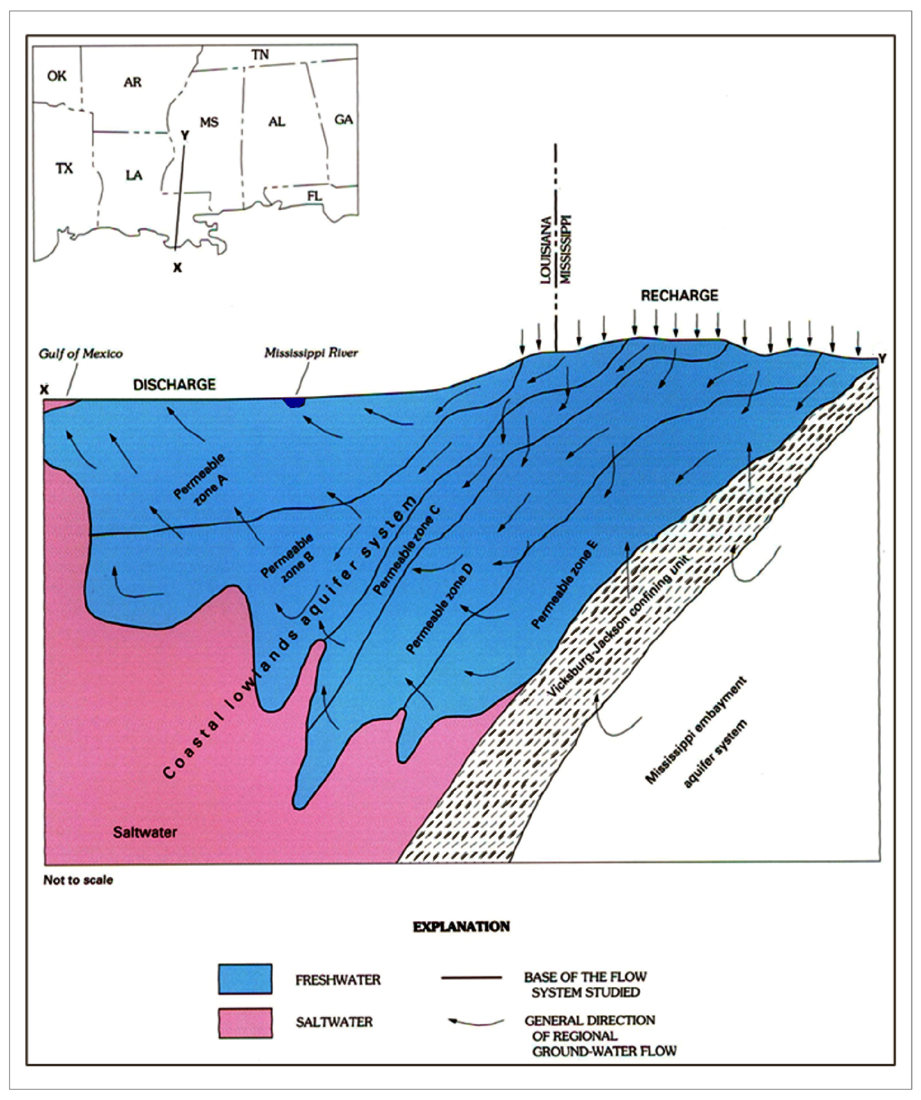
According to [24], the CLAS is divided into five permeable zones and two confining units to evaluate flow distribution. The lack of regionally continuous confining layers complicates the distinction between individual aquifers [25]. The system is underlain by the Jackson and Vicksburg Groups, which together form the Vicksburg–Jackson confining unit as shown in Figure 2 [23]. These geological groups comprise substantial deposits of clay, silt, and limestone formed during the most recent major marine transgression, spanning the late Eocene to Oligocene epochs. The upper portions of these groups contain extensive sand layers that serve as aquifers and are part of the CLAS. Recharge primarily results from precipitation infiltrating elevated areas and the landward margin of the system. Following recharge, groundwater moves downgradient toward coastal regions and laterally toward the Mississippi River. Groundwater ultimately discharges to streams, wetlands, and, in the southernmost areas, the Gulf of Mexico [25].
Extensive agricultural and industrial development in the area has supported rapid population growth and increased demand for both groundwater and surface water resources [27]. Consequently, groundwater extraction for municipal, industrial, agricultural, and domestic purposes is widespread across the study area [23]. Intensive withdrawals from the aquifer system in certain locations have caused saltwater intrusion and land subsidence [28]. Groundwater level declines of approximately 61 m due to increased pumping, which is more than tenfold between 1930 and 1970 [28].

2.2. Datasets

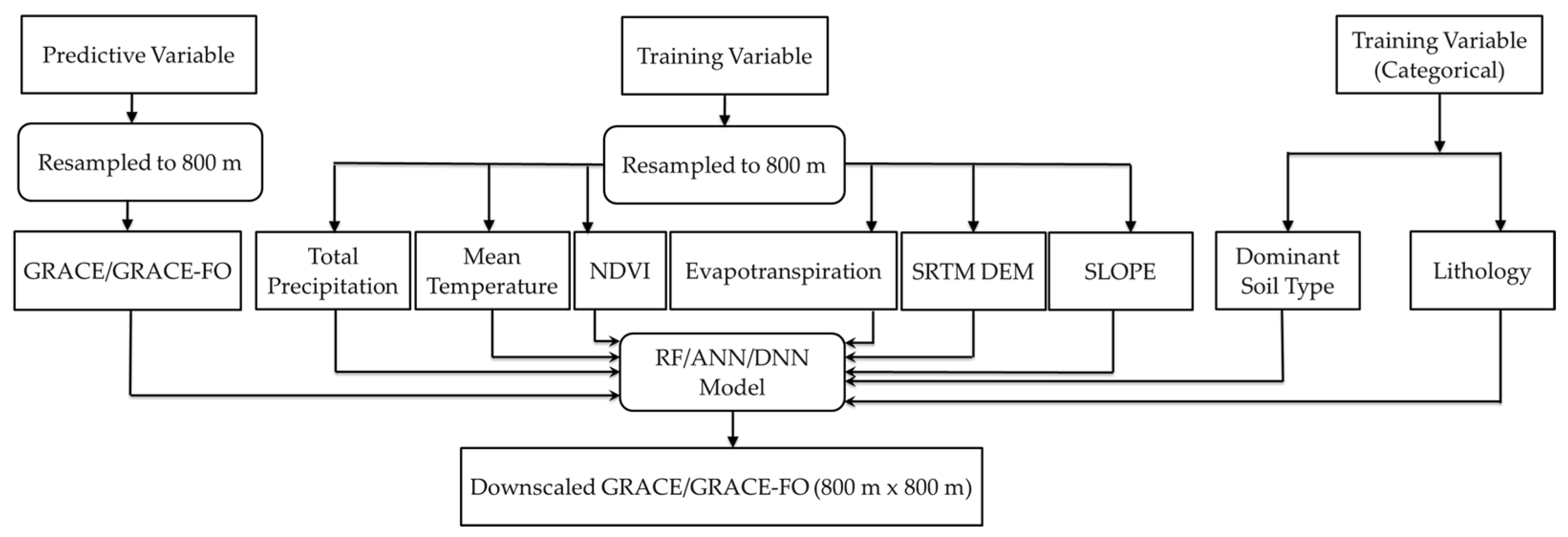
We drew on eight unique data layers as inputs, weaving in the 2003–2023 monthly GRACE/GRACE-FO layer at its native resolution for the RFM, ANN, and DNN models. Table 1 presents the data types along with their corresponding spatial resolutions. Below, you will find a brief overview of each layer. We carefully aligned all datasets with each month of the 2003–2023 GRACE/GRACE-FO record. Figure 3 illustrates the downscaling approach.

2.2.1. GRACE/GRACE-FO

This study used Level 3 processed RL06v04 version products of GRACE images from 2003 to 2016, as well as RL06.1v04 version products of GRACE-FO images from 2019 to 2023. GRACE data from 2017 and GRACE-FO data from 2018 were excluded due to reduced quality during the GRACE mission’s end and the initialization phase of GRACE-FO. According to [29], the monthly land mass grids represent water mass anomalies ex-pressed as equivalent water thickness, which was derived from specified timespan’s GRACE and GRACE-FO time-variable gravity observations data relative to the specific time-mean reference period. Water density (1000 kg/m3) was used to convert equivalent water height. The liquid water equivalent thickness (LWE) represents the TWS anomalies from soil moisture, snow, surface water (rivers, lakes, reservoirs), as well as groundwater. A glacial isostatic adjustment (GIA) correction has been applied. Standard corrections for geocenter (degree-1), C20 (degree-20), and C30 (degree-30) are also incorporated in this version. Post-processing filters have been employed to mitigate correlated errors. Version 04 (v04) of terrestrial water storage data incorporates enhanced and consistent C20 and Geocenter corrections. Additionally, an ellipsoidal correction has been integrated to accommodate Earth’s non-spherical shape when translating gravity anomalies into surface mass change. This RL06.1 represents an updated release compared to the previous RL06, with the only distinction being the utilization of Level-1B accelerometer transplant data for the GF2 (GRACE-FO 2) satellite in RL06.1, which employs the ACH data product. The data grids are available in ASCII, netCDF, and GeoTIFF formats. GRACE products in ASCII format for RL06 and beyond version have taken on the YAML encoding header, which is in full agreement with the PODAAC metadata best practices [30]. In this study, GRACE mascon data are provided on a 1° (~111 km) grid; however, the effective spatial resolution of the signal is coarser, approximately ~300–330 km [29]. The TWSA is expressed in LWE or equivalent water height (EWH). The unit of the LWE is the meter. Time mean (1 January 2005 to 31 December 2010) LWE value was removed from the monthly LWE of GRACE and GRACE-FO to produce the monthly TWSA [29].
A sensitivity analysis was conducted to evaluate the potential impact of the 2017–2018 GRACE/GRACE-FO data gap on long-term trend estimation. The trend slope of TWSA for 2003–2023 was calculated under two scenarios: (i) excluding the data gap from the original dataset, and (ii) filling the missing period using linear interpolation between the final GRACE observation and the initial GRACE-FO observation. The analysis demonstrates that the estimated trend slope remains constant (−0.07 cm/year) in both scenarios, with a difference of 0.00%. This finding suggests that omitting the data gap has a negligible effect on long-term trend estimation.

2.2.2. Temperature and Precipitation

Monthly total precipitation and mean temperature data for the study area from 2003 to 2023 were obtained from the Parameter-elevation Regressions on Independent Slopes Model (PRISM) dataset [31]. PRISM provides daily and monthly climate data at approximately 800-m spatial resolution for the United States. Precipitation is reported in millimeters and temperature in °C.

2.2.3. NDVI

The NDVI is a remote sensing metric that quantifies vegetation density and health within a defined region. NDVI is derived by comparing reflectance values of near-infrared (NIR) and red (RED) wavelengths captured in satellite imagery:
N D V I = N I R R E D N I R + R E D
NDVI data for the study area from 2003 to 2023 were obtained from NASA’s Moderate Resolution Imaging Spectroradiometer (MODIS). This dataset enables quantitative assessment of vegetation health and growth dynamics over time. The Terra MODIS (MOD13A1) version 6.1 NDVI product provides 500-m spatial resolution and 16-day temporal resolution [32].

2.2.4. ET

ET data for the study area, covering the period from 2003 to 2023, were sourced from the NASA Earthdata Forum. The MODIS on the Terra satellite provides the MOD16A2 version 6.1 ET product, which offers 500-m spatial resolution and eight-day temporal resolution [33].

2.2.5. DEM and Slope

Elevation data with a 30-m resolution was obtained from the Shuttle Radar Topography Mission (SRTM) Digital Elevation Model (DEM) [34] available through the EarthExplorer data portal “https://earthexplorer.usgs.gov/ (accessed on 4 May 2023)”. Slope values were calculated for each pixel of the SRTM DEM.

2.2.6. Soil Type

Digital soil type data were obtained from the Food and Agriculture Organization/United Nations Educational, Scientific, and Cultural Organization (FAO/UNESCO) soil map version 3.6, completed in 2003. The digitized map was corrected for database and line errors [35]. The study area is characterized by fourteen dominant soil units, including Ferric Acrisols (Af), Gleyic Acrisols (Ag), Orthic Acrisols (Ao), Cambisols (B), Gleysols (G), Phaeozems (H), Kastanozems (K), Luvisols (L), Histosols (O), Gleyic Podzols (Pg), Regosols (R), Chromic Vertisols (Vc), Pellic Vertisols (Vp), and Planosols (W).

2.2.7. Lithology

Lithological data for the study area were obtained from the Esri dataset [36], which has a spatial resolution of 250 m. It has ten classes. The classes are Unconsolidated sediment (Us), Siliciclastic Sedimentary Rock (Ss), Mixed Sedimentary Rock (Ms), Carbonate Sedimentary Rock (Cs), Evaporite (E), Intermediate Volcanics (Iv), Basic Volcanics (Bv), Acid Plutonics (Ap), Basic Plutonics (Bp), and Metamorphic Rocks (M).

2.2.8. Ground-Based Measurement

Groundwater represents a major component of TWS. This study compares the trends of downscaled 800-m TWSA with groundwater level anomaly (GWLA) trends. The comparison is based on analyzing the similarity and differences between TWSA and GWLA trends using groundwater level (GWL) data collected from 2003 to 2023 at multiple monitoring sites. Data sources include the Texas Water Development Board (TWDB), the United States Geological Survey (USGS), the Mississippi Department of Environmental Quality (MSDEQ), the Geological Survey of Alabama (GSAL), and the Florida Department of Environmental Protection (FLDEP). The United States Geological Survey also provided access to daily groundwater level data through the National Groundwater Monitoring Network (NGWMN) portal [37].

2.3. Data Preprocessing

2.3.1. Process Source Data

After downloading the source data from the respective sources, all datasets were converted into Tagged Image File Format (TIFF). TIFF can store various data types, including integer and floating-point values, and can also hold multi-band imagery [38]. After that, all study datasets were projected into the UTM Zone 16N NAD 1983 (EPSG: 26916) coordinate system [39]. For the dynamic variables, the NDVI and ET data provided eight-day and sixteen-day composites from 2003 to 2023. Different spatial analysis tools of ArcGIS Pro 3.6.0 (Esri, Redlands, CA, USA) were used to aggregate the data and generate the monthly mean of NDVI and ET from 2003 to 2023.
The GRACE/GRACE-FO satellite data provides the anomaly of the TWS for each month. The time mean (1 January 2005 to 31 December 2010) LWE value was removed from the monthly LWE of GRACE/GRACE-FO to produce the monthly TWSA. The anomalies of training variables, including precipitation, temperature, NDVI, and ET, were also prepared. These were related to the changes in TWSA for each month from 2003 to 2023. For example, each month’s APT of 2023 was prepared by deducting the time mean total precipitation from each month’s total precipitation in 2023. The time mean total precipitation was calculated as the mean of the monthly totals from 1 January 2005 to 31 December 2010. Similarly, ATM, ANDVI, and AET were prepared for each month from 2003 to 2023.
Each raster layer was clipped to the study area border. Subsequently, the layers were resampled to match the approximately 800-m resolution of the PRISM data. The Nearest Neighbor resampling method was applied to GRACE/GRACE-FO, NDVI, and ET data from 2003 to 2023, as well as to the digital elevation model (DEM), slope angle, and lithology layers. In the absence of direct 800-m TWS observations, GRACE pixel values are used as the statistical learning target, consistent with prior studies in the field. It is important to note that this approach represents statistical downscaling rather than true physical downscaling, as the coarse-resolution GRACE signal is disaggregated to finer scales. To mitigate the risk of spatial overfitting, train/test splitting was performed via random pixel sampling, and the downscaled output was cross-validated against independent groundwater level observations. After converting the soil type polygon layer into TIFF file type, the majority resampling method was used.

2.3.2. Prepare Model Inputs

A fishnet [40] was created to span the study area and align with the 800-m dimensions of the dependent training variables. Prior to this, point databases were prepared, with each row representing the pixel value of all variables for each month within a single year. The spatial join tool was used to extract values from each point in the input database layer, which were then integrated into the Fishnet vector. This process associated data from each point with the corresponding cell in the Fishnet vector, resulting in a new vector layer containing values from each input layer within the study area. These values were prepared for subsequent model input. In total, 19 fishnets were produced. Each row of every Fishnet recorded the monthly APT, monthly ATM, monthly ANDVI, monthly AET, digital elevation model (DEM) value, slope value, dominant soil type, and lithology for a single year. For instance, each row of the 2006 Fishnet included the monthly APT, ATM, ANDVI, and AET for 2006, as well as DEM value, slope value, land cover, dominant soil type, and lithology. Appendix A presents the first ten rows of the 2006 Fishnet. To ensure consistency, any cell containing no data was removed from each Fishnet. Each Fishnet was subsequently uploaded to Google cloud for use in the RF, ANN, and DNN models on the Google Colab platform.

2.4. Models

Three models—RF, ANN, and DNN—were developed to downscale the TWSA from GRACE/GRACE-FO satellite imagery to a spatial resolution of into 800 m. All the models were developed with a total of nine datasets. All the models were implemented and executed using Google Colab platform. Google Colab with Python 3.12.13 and Jupyter Notebook 6.5.7 is a free cloud-based platform developed by Google that allows users to write and execute Python code in a Jupyter Notebook environment through a web browser. It supports real-time collaboration, seamless integration with Google Drive, and provides access to computational resources such as graphics processing units (GPUs) and Tensor Processing Units (TPUs), making it especially suitable for ML, data analysis, and geospatial research [41]. All experiments were conducted using Google Colab Pro with GPU-enabled environments. Due to the dynamic nature of Colab sessions, the exact hardware configuration (e.g., GPU/TPU type and RAM) may vary between runs. Colab no-setup interface and built-in support for popular Python libraries like TensorFlow, NumPy, and Pandas have made it widely adopted in both academic and applied research contexts.
The RF model was built using the scikit-learn 1.6.1 [42] Python ML library. Scikit-learn is a widely used ML library that provides a broad set of algorithms for classification, regression, and clustering. It is designed to integrate seamlessly with core Python scientific libraries such as Matplotlib 3.10.0, Seaborn 0.13.2, and GeoPandas 1.1.3. For geospatial data analysis, the GeoPandas library was employed, which extends the functionality of pandas to enable the handling of geometric objects like points, lines, and polygons [43]. To visualize model outputs and spatial patterns, Matplotlib and Seaborn were used for creating both static and statistical plots. In addition, other geospatial libraries like Shapely 2.1.2, Fiona 1.10.1, and Pyproj 3.7.1 were used to support the implementation of the RF model. Shapely was used for geometric operations on vector data [44], Fiona for reading and writing spatial vector data formats such as shapefiles, and Pyproj for performing coordinate system transformations and geospatial projections [45].
ANN and DNN models were developed using the Keras 3.13.2 Python ML library [46]. Keras is a high-level deep learning Application Programming Interface (API) written in Python, designed to be user-friendly, modular, and extensible, making it well-suited for building and training neural network models. It is among the most widely adopted frameworks for developing neural network-based learning systems. In addition to Keras, several other Python libraries like Scikit-learn, GeoPandas, Matplotlib, Seaborn, Shapely, Fiona, and Pyproj were used to support the implementation and execution of the ANN and DNN models, particularly for data preprocessing, geospatial analysis, and visualization tasks.
For each model, the input dataset was randomly split into 80% training and 20% testing subsets using Scikit-learn’s train_test_split with a fixed random state (random_state = 42), a common procedure to assess generalization performance on unseen data [47]. Predictor variables were preprocessed prior to model training. Categorical variables (lithology and soil) were transformed using one-hot encoding, while continuous variables were standardized using StandardScaler [48] to ensure consistent scaling and reduce numerical instability during training. Model performance was evaluated using the coefficient of determination (R2) and root mean square error (RMSE).
Hyperparameter selection for all models was performed through iterative testing by evaluating model performance across different configurations. Model performance was evaluated using an independent test dataset, and cross-validation was not applied in the present study.

2.4.1. Random Forest

RF is an ensemble technique rooted in decision trees, characterized by its non-parametric nature. It employs randomization during the process of selecting features at each node and can be used for both classification and regression tasks [13,49,50,51]. According to Breiman et al. [52] clarifies that RFM blends the collective outcomes of all decision trees within each forest with the randomly selected vectors for the predictor variables. The RF model was implemented in Python using the RandomForestRegressor function from the Scikit-learn library. In this study, the model was trained using 100 decision trees (n_estimators = 100) with a maximum depth of 15 (max_depth = 15) and a fixed random seed (random_state = 42) to ensure reproducibility.
The RF model uses bootstrapping with replacement to generate multiple subsets of the training data and constructs individual regression trees based on the Classification and Regression Trees (CART) algorithm [51]. RF applies bootstrapping with replacement to create multiple subsets of the original training data. At each node, a random subset of predictor variables is selected, which helps reduce overfitting and improves model generalization.
The ultimate prediction output can be derived by taking the average of predictions produced by each individual regression tree [53]:
f = 1 N i = 1 N f i x ,
where N is the number of trees and fi(x) is the prediction of the i-th tree [51].
Feature importance was extracted from the trained model to assess the relative contribution of predictor variables to TWSA estimation.

2.4.2. Artificial Neural Network

An ANN model consists of interconnected layers of artificial neurons (nodes), which process data inputs and learn patterns through training. ANN models are made up of numerous interconnected nodes (or neurons) [54]. Each node applies an output function, known as the activation function, which determines the output of that node. The connection between any two nodes carries a weight, often referred to simply as the “weight”, which represents the strength or influence of the signal traveling through it and serves as the memory of the ANN [55]. The network’s output depends on the connections between nodes, the values of these weights, and the choice of activation function.
In this study, we have developed a feed-forward back-propagation ANNs approach to downscale GRACE data. We determined the right number of hidden layers by evaluating the R2 values, a measure that helps us see how well the model fits the data. For this study, two hidden layers with 64 and 32 nodes were selected to compute the ANN model. The Rectified Linear Unit (ReLU) activation function was applied in the hidden layers, while a linear activation function was used in the output layer for continuous prediction.
The model was compiled using the Adam optimizer (with default learning rate) and mean squared error (MSE) as the loss function, with mean absolute error (MAE) included as an additional evaluation metric. The ANN model was trained for 100 epochs with a batch size of 32 and a validation split of 0.2.
Prior to training, categorical variables were converted using one-hot encoding and continuous variables were standardized. Model performance was evaluated using R2 and RMSE on the independent test dataset. Feature importance was estimated using permutation importance with an MLPRegressor model configured with a similar hidden-layer structure.

2.4.3. Deep Neural Network

Deep Neural Networks (DNNs) are an advanced type of ANN characterized by the presence of multiple hidden layers between the input and output layers. These models are designed to automatically learn hierarchical features from the input data [56]. In this study, ANN and DNN models were constructed using the Keras Sequential API [46]. The DNN architecture consisted of five hidden layers comprising 128, 64, 64, 32, and 16 neurons, respectively. All hidden layers used the ReLU activation function, while the output layer used a linear activation function for regression.
The model was compiled using the Adam optimizer (default learning rate) and mean squared error (MSE) loss, with mean absolute error (MAE) as an additional metric. Training was performed for 100 epochs with a batch size of 32 and a validation split of 0.2.
Similar to the ANN model, predictor variables were preprocessed using one-hot encoding and standardization prior to training. Model performance was evaluated using R2 and RMSE on the test dataset. The R2 score measures the proportion of variance in the dependent variable that is predictable from the input features, indicating how well the model fits the observed data [57]. Permutation-based feature importance was estimated using an MLPRegressor surrogate model with an equivalent architecture.
The DNN architecture was selected through iterative testing by evaluating model performance (R2 and RMSE), rather than through formal hyperparameter optimization.

3. Results

After the successful completion of the RF, ANN, and DNN models, each model provided the 800-m monthly downscaled TWSA from 2003 to 2023 using data from the GRACE/GRACE-FO satellites. Within the three models, the DNN model took the longest time to execute. On the other hand, the RF model took a shorter time compared to the other two models. After the successful completion of each month’s downscaling by RF, ANN, and DNN models, the error metrics of the model’s output are calculated. Table 2 presents the error metrics of the RF, ANN, and DNN models.
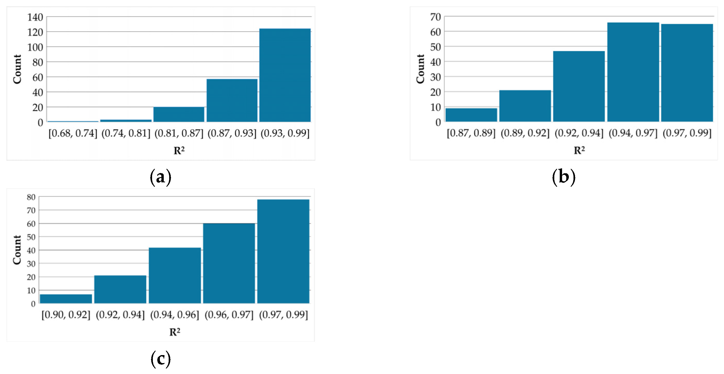
From Table 2, the DNN model outperformed the other two models. The R2 value of the monthly downscaled TWSA by DNN ranges from 0.901 to 0.992. In comparison, the R2 value for RF ranges from 0.689 to 0.993. The ANN model also performed strongly, with R2 values between 0.869 and 0.989. To illustrate the distribution of R2 values, Figure 4 presents histograms for the downscaled monthly TWSA using RF, ANN, and DNN. In Figure 4, the RF histogram shows that, with few exceptions, most downscaled products have an R2 value between 0.81 and 0.99. By contrast, the histograms for ANN and DNN demonstrate their strong performance in downscaling TWSA from 2003 to 2023 using GRACE/GRACE-FO data. The RF model shows a distribution concentrated at higher R2 values (0.93–0.99), with a noticeable tail toward lower values. The minimum R2 (0.689) occurred in April 2007. This reduction in performance appears to be tied to specific-month variability in the predictor–response relationship, not a regular seasonal pattern. During this time, the link between the input variables and TWSA likely strays from the main patterns captured in the training data. As a result, nonlinearity increases and model generalization drops. This behavior matches the known characteristics of Random Forest models, which perform poorly when the predictor–response relationship falls outside the range of the training dataset [52]. In contrast, ANN and DNN models show more stable performance over time. Their R2 distributions are narrower and more concentrated. Additionally, the low RMSE for all three models indicates a good fit and reliable predictions (Table 2). The achieved RMSE values (~0.002–0.019 m, i.e., 2–19 mm) are comparable to or lower than the typical uncertainty range of GRACE observations (on the order of a few centimeters, ∼20–30 mm) [58], suggesting that the downscaling approach does not introduce substantial additional error beyond the inherent satellite uncertainty.
To further support model comparison, spatial evaluation metrics were computed, including spatial Pearson correlation and Structural Similarity Index (SSIM) for all monthly outputs. The summary statistics of these metrics are presented in Table 3.
The results indicate that all models exhibit strong spatial agreement with the original GRACE data (r > 0.95; SSIM > 0.90). Among the models, the DNN shows slightly higher mean spatial correlation and SSIM values, while the ANN also demonstrates consistently strong spatial performance across the study period.
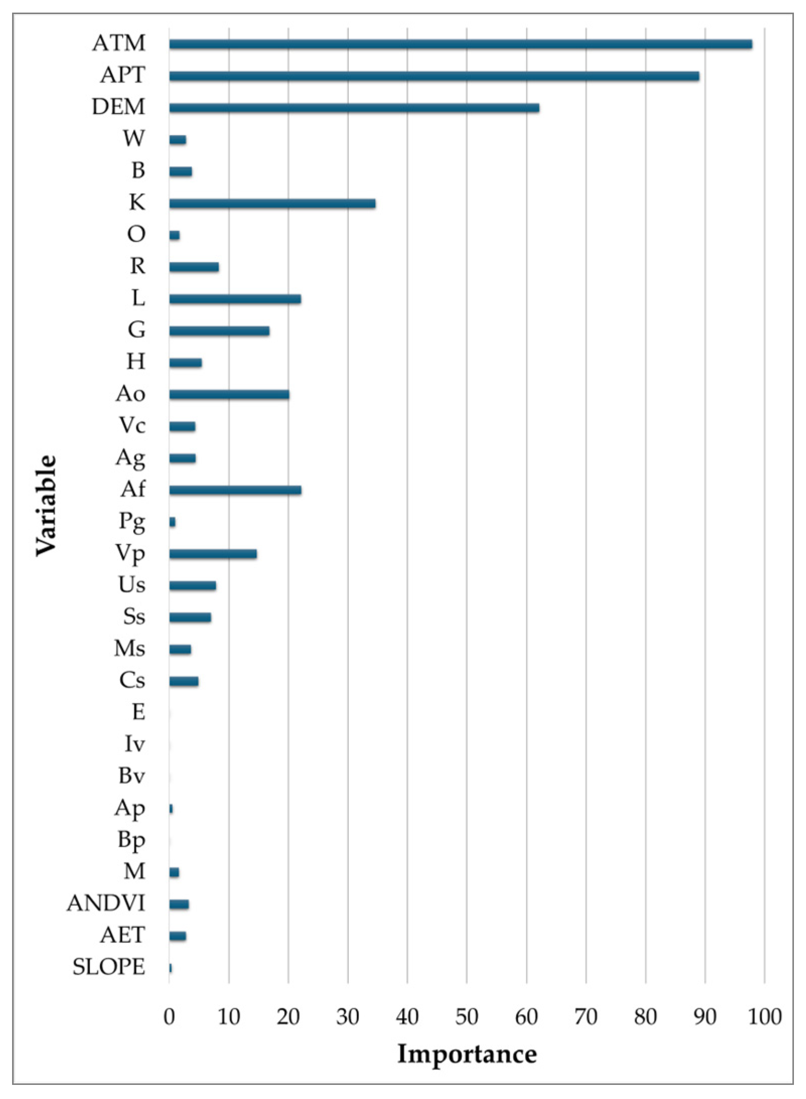
Each model generated a ranking table of variable importance after completing the downscaling of GRACE/GRACE-FO data for each month. RF, ANN, and DNN models produced consistent rankings of variable importance in monthly downscaled TWSA outputs. All three models identified ATM, APT, DEM, and soil as the most important variables for downscaling TWSA to 800 m. In contrast, slope was consistently the least important variable. Figure 5 summarizes the variable importance ranking by the ANN model.
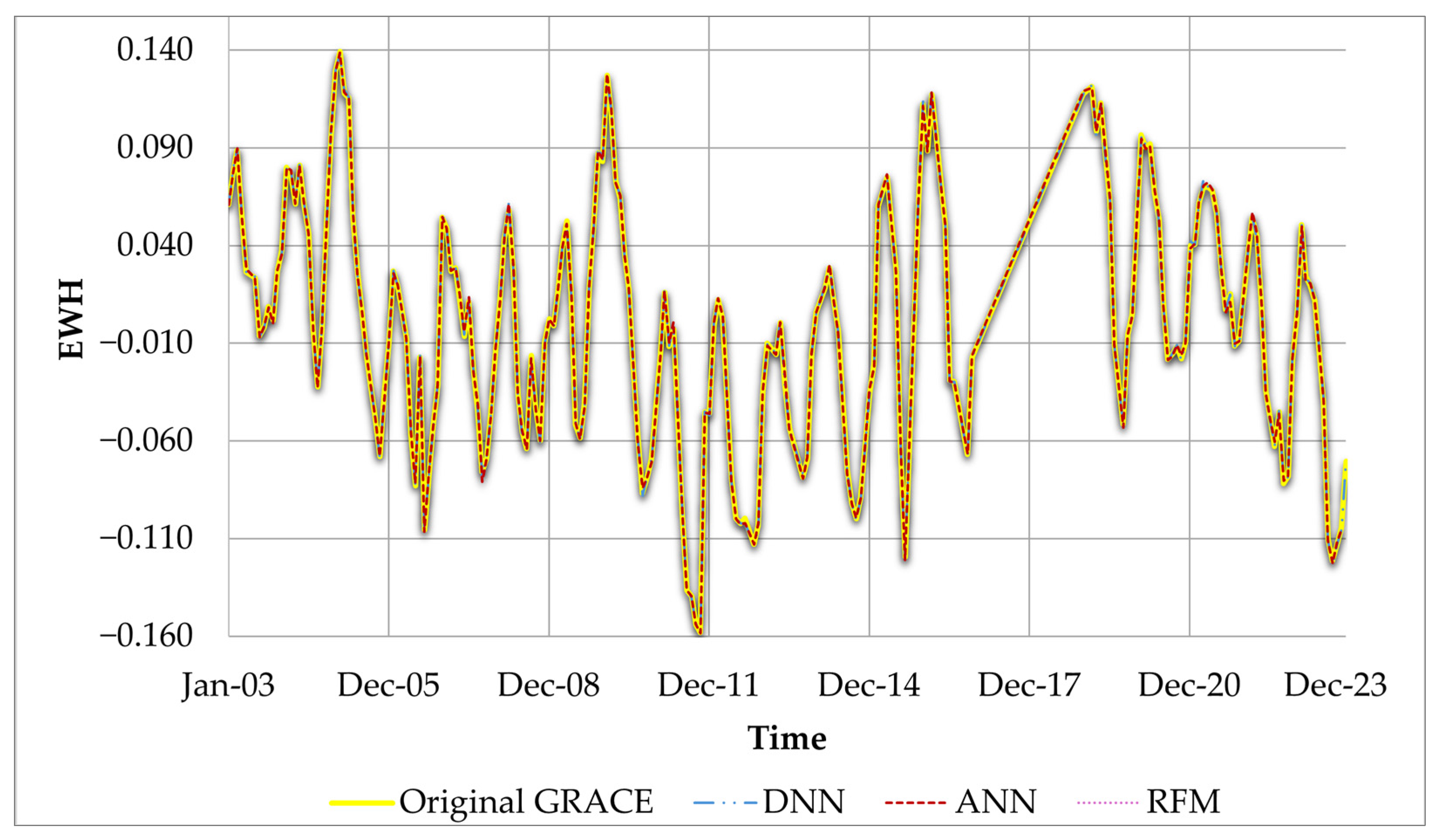
Model validation is a critical step for comparing outputs with established datasets. However, comparing the downscaled GRACE/GRACE-FO dataset is challenging, as no directly comparable observed dataset exists. Therefore, the most suitable approach was to analyze EWH variations in the generated timeseries for the study area. This method enables evaluation of mass change regionally [15,59]. For each model, a timeseries value for each timestep was calculated by averaging the values of all grid cells. Figure 6 shows the time series for the ML models and original GRACE data. At certain time steps, the model outputs deviated minimally from the original GRACE dataset. Overall, no distinct patterns emerged in the model outputs; all models consistently reflected the trend of the GRACE dataset.
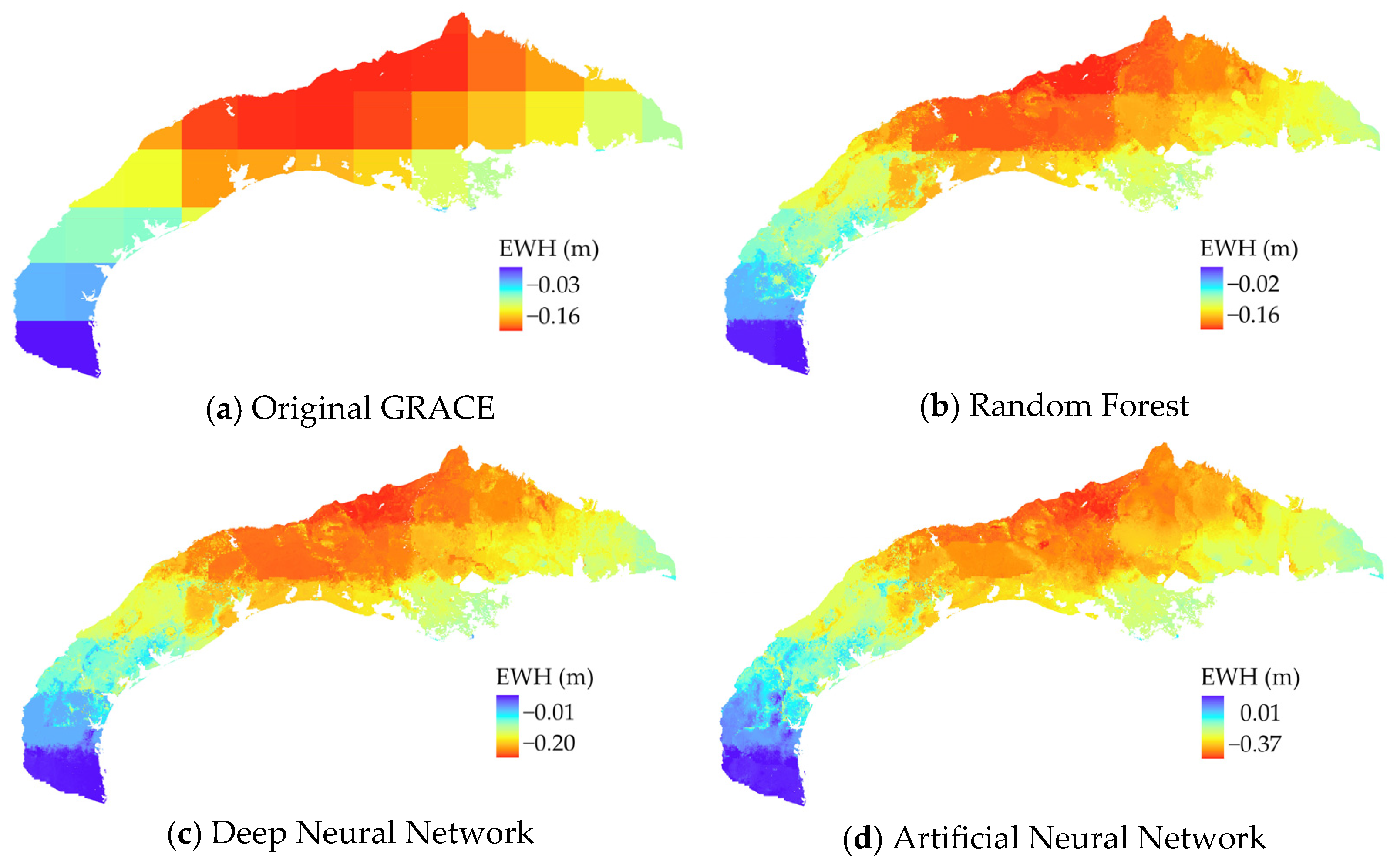
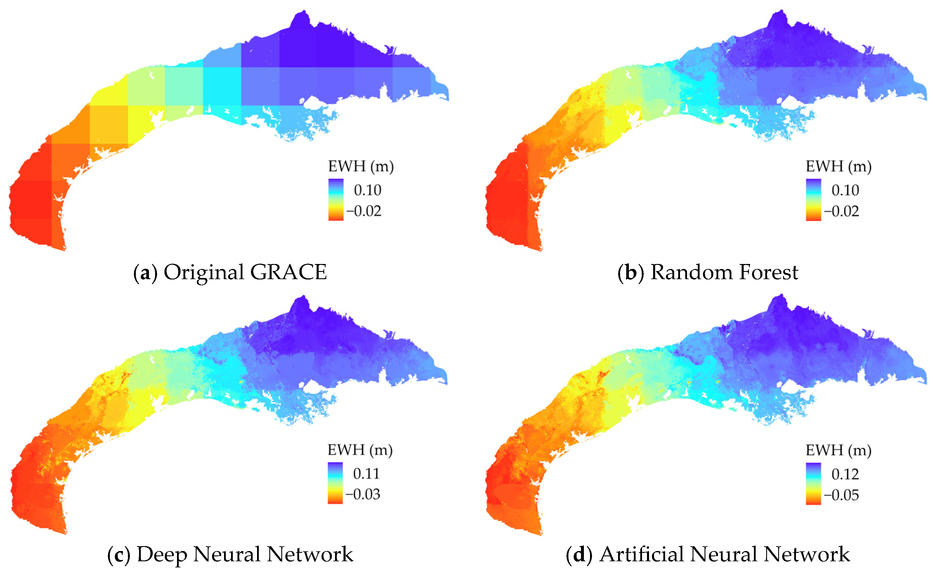
The model metrics and time series metrics of all three models suggest a statistically sound model. Although the DNN model achieved slightly better statistical performance (higher R2 and lower RMSE) compared to the ANN, this improvement was marginal and did not translate into better spatial representation. Visual inspection of the model output remains an important criterion in determining which model most effectively assesses the TWS of the study area. Specifically, visual inspection indicates that the ANN performed well, showing a reasonably consistent spatial distribution. Although the output values of the ANN model were higher, the overall trends aligned well with those of the original dataset. In contrast, most outputs from RF and DNN exhibited a very inconsistent spatial distribution. While the overall output values of RF and DNN were close to those of the original dataset, these models appeared to be very sensitive to the input training variables. In particular, RF and DNN outputs tend to retain characteristics of the coarse-resolution GRACE signal, suggesting limited representation of sub-grid variability. These observations are consistent across the majority of monthly datasets, indicating that the improved spatial coherence of the ANN model is not limited to isolated cases. Although Table 3 shows that the DNN model achieves slightly higher spatial correlation and SSIM values, these global metrics do not fully capture localized spatial inconsistencies and sensitivity to input variables observed in the RF and DNN outputs. To illustrate these findings, Figure 7 and Figure 8 present a comparison of the visual outputs of the ML models with the original GRACE data at two different times: September 2015 and February 2023. In both cases, it is evident that the ANN performed well and was visually more realistic than the RF and DNN models.
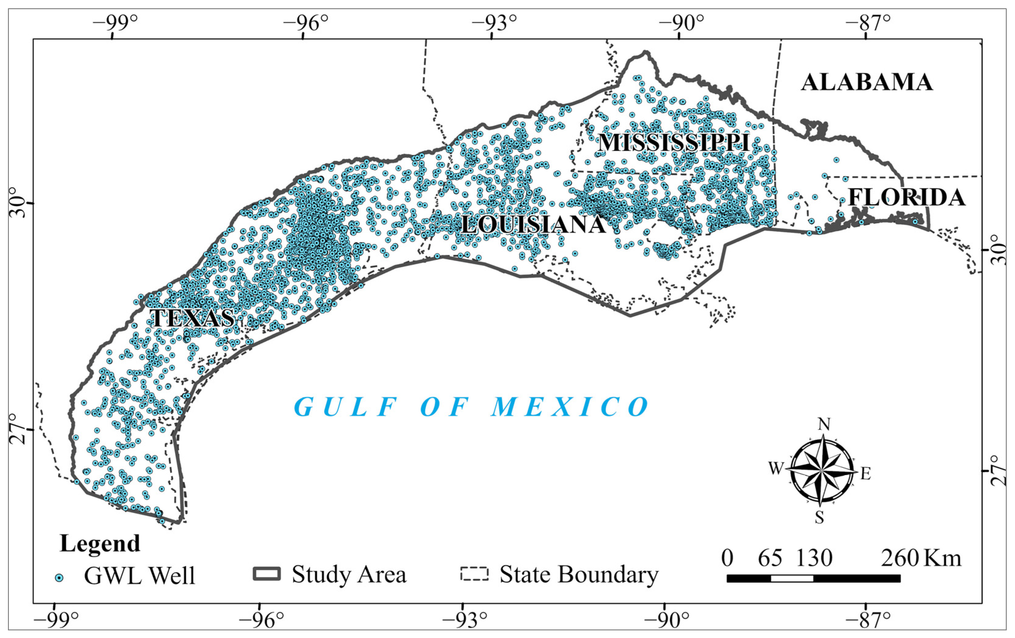
To validate the model output, another attempt was made to compare the temporal trends of downscaled 800-m TWSA with groundwater level anomaly (GWLA) trends. Groundwater is a primary contributor to TWS. Any change in GWL within specific timesteps should be reflected in the area’s TWSA. Downscaled TWSA by ANN from 2003 to 2023 was employed for this analysis. Correspondingly, the GWLA surface was generated using daily GWL data from multiple organizations. A total of 4242 GWL monitoring wells were used for this purpose. The well observations were first aggregated to annual mean groundwater levels to ensure temporal consistency with the downscaled TWSA dataset. Each year, a GWL surface was generated from available data from these wells. Figure 9 shows the distribution of GWL monitoring wells across the study area. It should be noted that Figure 9 represents the cumulative distribution of wells over the entire study period (2003–2023), and not all wells were available in every year. Groundwater level surface maps from 2003 to 2023 were generated using annual mean groundwater levels derived from daily observations. The spatial Inverse Distance Weighted (IDW) tool in ArcGIS Pro interpolated groundwater surfaces from 2003 to 2023 using the data. Similarly, a baseline groundwater surface map for the period 2005–2010 was generated, using mean groundwater levels calculated from daily observations between 1 January 2005 and 31 December 2010. Subsequently, GWLA maps from 2003 to 2023 were created by subtracting the 2005–2010 groundwater surface from those of 2003–2023.
It is important to note that the downscaled TWSA represents integrated terrestrial water storage (including groundwater, soil moisture, and surface water), whereas GWLA reflects only groundwater level variations rather than groundwater storage. Therefore, direct quantitative comparison between the two datasets is limited. Furthermore, due to the absence of physically observed high-resolution time series TWS data, direct validation at fine spatial scales is not feasible; therefore, a trend-based comparison with GWLA was adopted as an alternative evaluation approach.
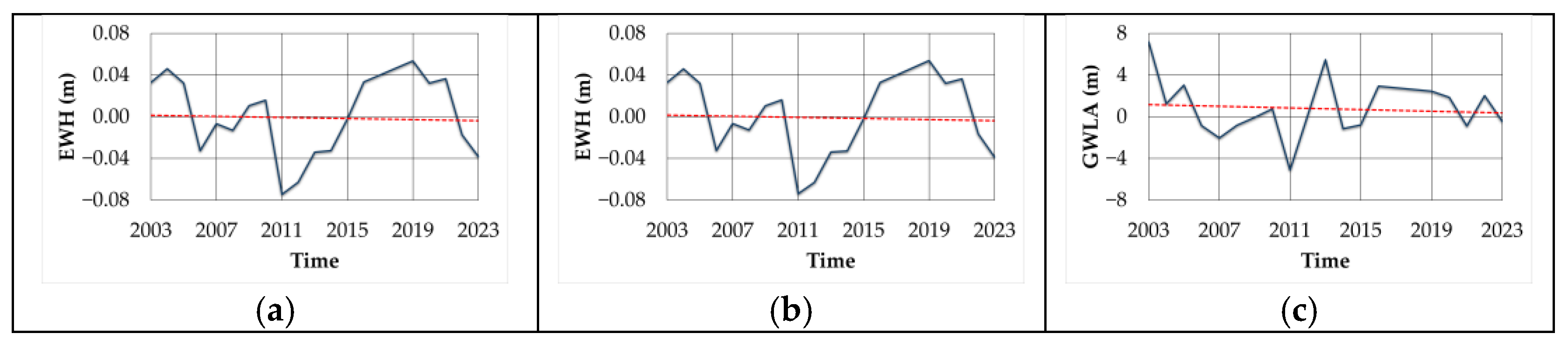
The validation was performed by comparing the temporal trends of spatially averaged GWLA and downscaled TWSA time series. To compare TWSA and GWLA trends, yearly mean ANN-based downscaled TWSA was plotted from 2003 to 2023, alongside GWLA values for the same period. In addition, the yearly mean original GRACE TWSA was plotted alongside the ANN-based downscaled TWSA to enable direct comparison of temporal trends between the datasets. Both graphical presentations show a decreasing trend (Figure 10), indicating consistency in temporal behavior between the datasets and supporting the reliability of the downscaled results. However, this agreement reflects similarity in long-term trends rather than a direct correspondence in magnitude and should therefore be interpreted as a qualitative validation rather than a strict quantitative comparison.

4. Discussion

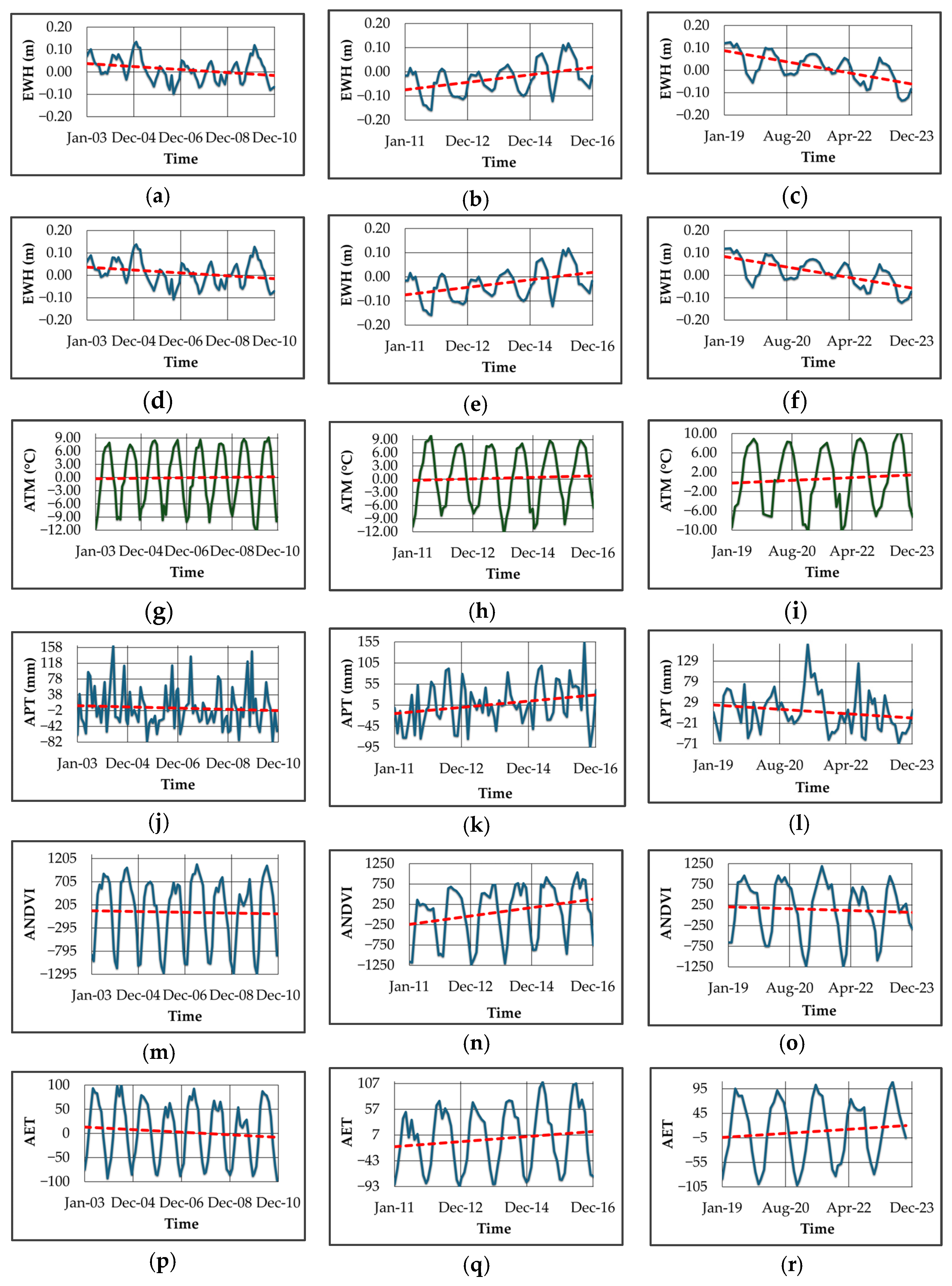
This study used two categories of variables, dynamic and static, to downscale GRACE/GRACE-FO satellite data to a spatial resolution of 800 m. Dynamic variables, including precipitation, temperature, ET, and NDVI, exhibit temporal variability and are measured at multiple time intervals. These variables capture temporal fluctuations and are critical for analyzing time-dependent processes [60]. In contrast, static variables such as elevation, slope, soil type, and lithology remain constant over time but may vary spatially. Sensitivity analysis was conducted to assess the impact of dynamic variables on the TWSA derived from GRACE/GRACE-FO data within the study area. Monthly mean TWSA values predicted by the ANN model were plotted for the period 2003–2023. Corresponding monthly mean values for the dynamic variables, specifically ATM, APT, AET, and ANDVI, were also plotted for the same period. In addition, the original GRACE equivalent water height (EWH) was included to enable direct comparison between GRACE-derived and ANN-based downscaled TWSA. The comparison indicates that the ANN-based downscaled TWSA follows the temporal behavior of the original GRACE EWH, confirming consistency between the datasets. For comparative analysis, all graphical profiles were discretized into three intervals: 2003–2010, 2011–2016, and 2016–2019, to facilitate trend comparison between dynamic variables and downscaled TWSA data (Figure 11).
In Figure 11, during the 2003–2010 time period, variables such as ATM exhibited an increasing trend. Meanwhile, the APT and ANDVI exhibited a decreasing trend. In addition, the AET showed a decreasing trend. This might be because reduced rainfall leads to declines in both soil moisture and groundwater recharge. As a result, with less water available, ET decreases, especially transpiration from stressed vegetation [9]. Consequently, in these timesteps, TWS decreased compared to the time mean (2005-JAN-01 to 2010-DEC-31) TWS value. Likewise, from 2019–2023, TWSA also showed a decreasing trend, while variables such as the APT and ANDVI exhibited a downward trend. Conversely, the ATM and AET exhibited an increasing trend. This suggests that it will create an impact in decreasing the TWS within these times. In contrast, TWSA increased from 2011–2016 timesteps. Normally, ET is a process that results in water loss. However, in these timesteps, ET showed an increasing trend. Notably, despite the increase in ET, stable temperature, increase in precipitation, and higher NDVI, the TWS of the study area increased within the timesteps from 2011 to 2016. The analysis demonstrates that dynamic variables, including ATM, APT, ANDVI, and AET are sensitive to changes in TWS within the study area. This relationship is evident in the variable importance rankings presented in Figure 5.
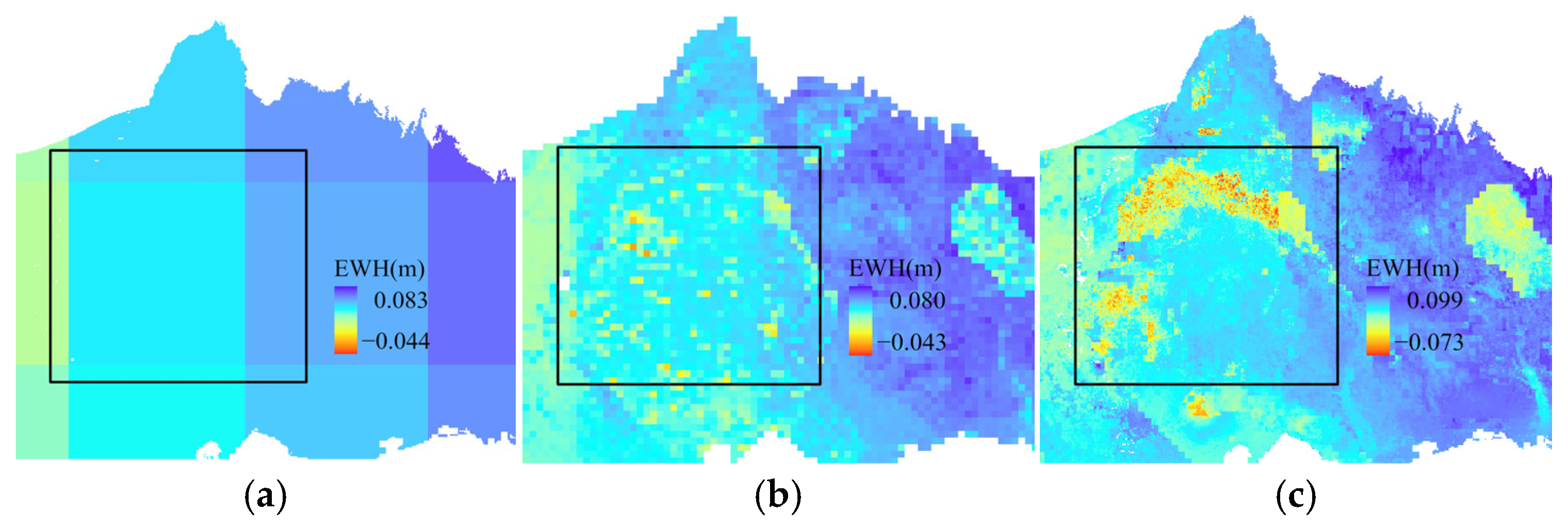
High-resolution TWSA data is becoming increasingly important in hydrology, water resources, and climate studies. In this study, ML approaches were employed to downscale the TWSA of GRACE/GRACE-FO satellite data to a resolution of 800 m. High-resolution TWSA provides the spatial detail necessary for groundwater regulations, agricultural planning, and sustainable water policy [4]. Figure 12 shows the comparison of the spatial details of downscaled 800-m TWSA data with original GRACE-FO data and downscaled 4 km TWSA data. The 4 km data was generated using the RF model [61]. From Figure 12, it is clear that downscaled 800-m TWSA can depict more details of TWSA distribution within the study area. This higher resolution helps identify localized hotspots of water depletion and recharge in the terrestrial environment. These localized patterns are consistent with the spatial variability of key environmental predictors (e.g., precipitation, temperature, evapotranspiration, and vegetation indices) and align with the temporal behavior of both the original GRACE data and GWLA trends, indicating that they represent physically meaningful hydrological features rather than artefacts introduced by the ANN model. Such detail enables more targeted mitigation strategies.
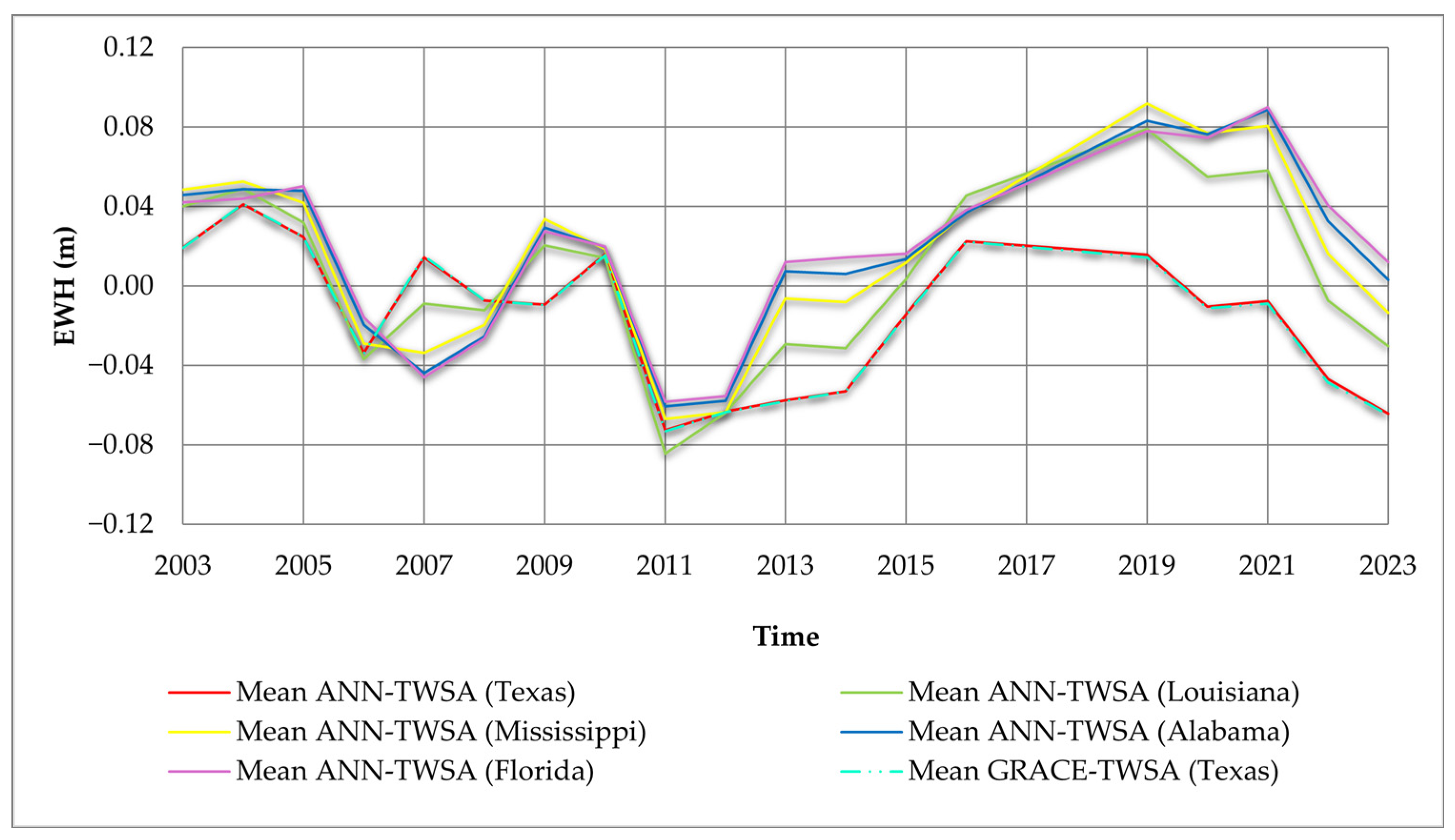
The CLAS comprises the coastal aquifers of Texas, Louisiana, Mississippi, Alabama, and Florida. An analysis was performed using the 800-m downscaled GRACE/GRACE-FO satellite data by ANN models to assess which portion of the aquifer system had greater water depletion compared to others within the time period 2003–2023. To perform this task, the downscaled TWSA data from 2003 to 2023 were subset using the state boundaries of Texas, Louisiana, Mississippi, Alabama, and Florida. Subsequently, a graphical representation of the yearly mean TWSA for Texas, Louisiana, Mississippi, Alabama, and Florida was generated (Figure 13). Figure 13 indicates that from 2003 to 2023, Texas experienced greater TWS depletion compared to the other states during most years. Additional comparison with the original GRACE TWSA (e.g., Texas region) shows that the temporal profiles are nearly identical, indicating that the downscaling preserves the original signal while enabling enhanced spatial interpretation.
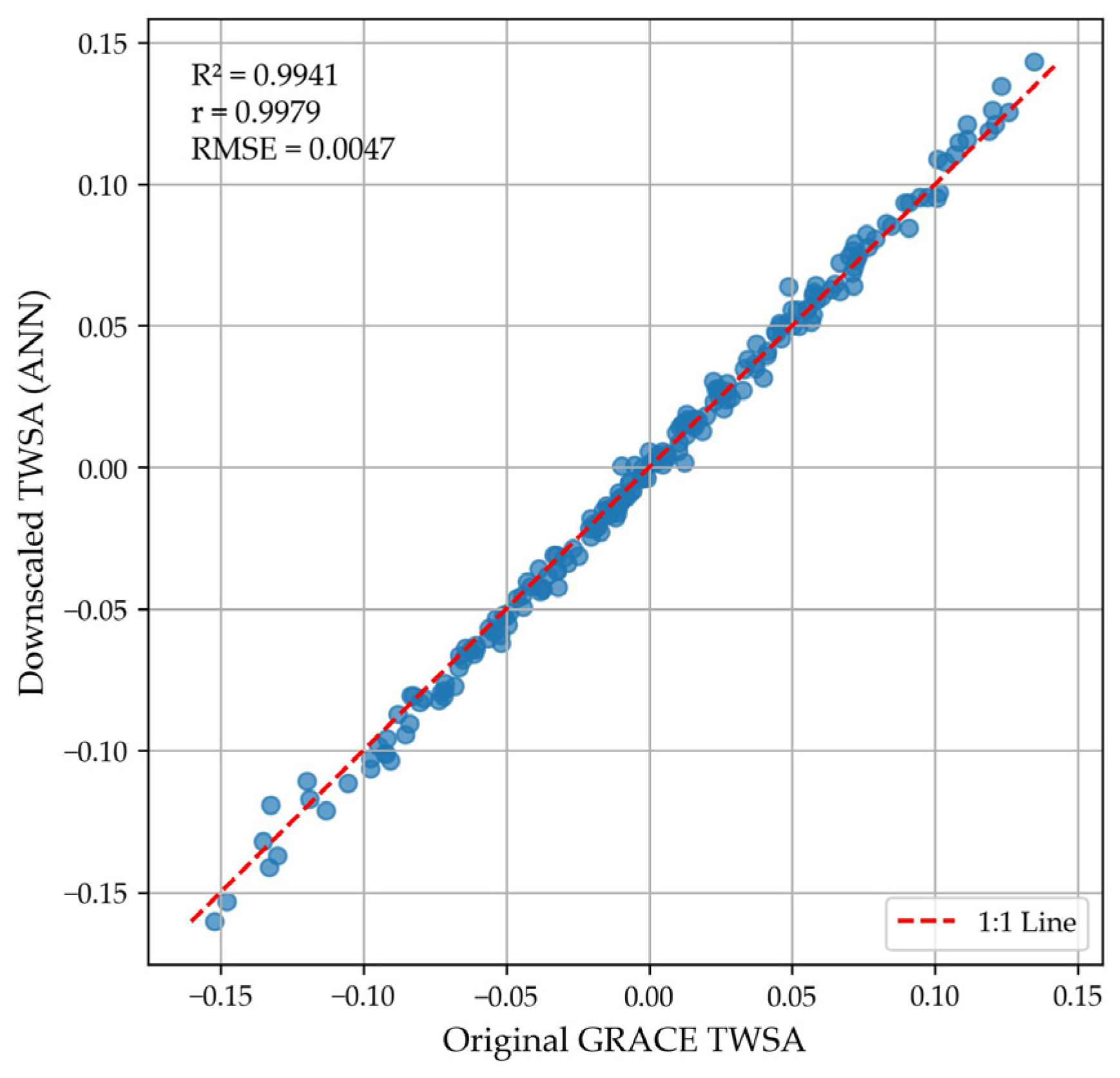
A comprehensive comparison between the original GRACE TWSA and the ANN-downscaled TWSA, aggregated to GRACE’s native resolution, was conducted using quantitative metrics and visual analysis. The datasets show strong agreement (R2 = 0.9941, r = 0.9979), low error (RMSE = 0.0047), and negligible bias (−0.0008). The scatter plot (Figure 14) further supports this, with points closely aligning along the 1:1 reference line, indicating minimal deviation. These results demonstrate that the downscaled TWSA preserves the magnitude and temporal variability of the original GRACE signal while enhancing spatial resolution for regional analysis.
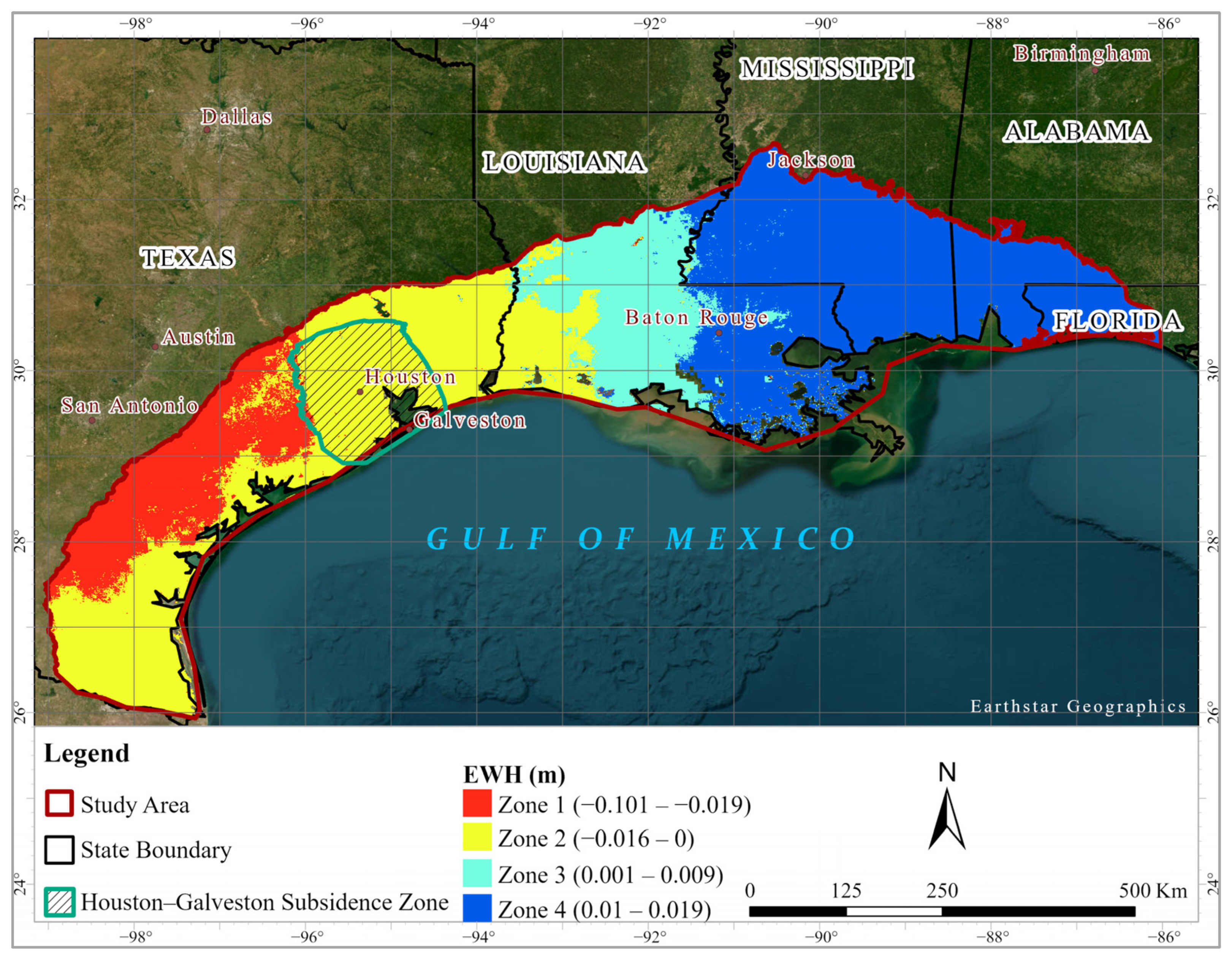
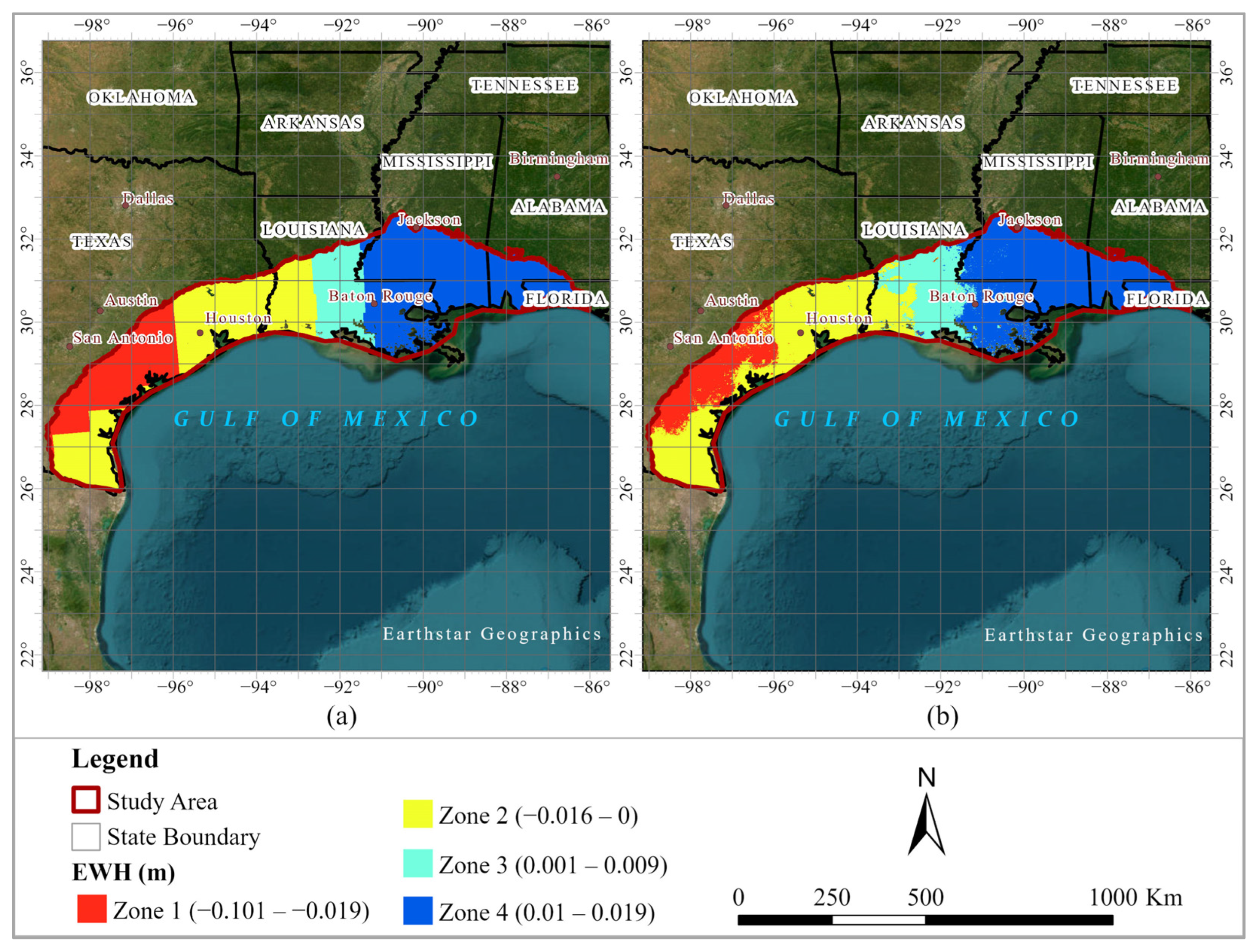
Finally, a TWS stress map for the period 2003–2023 was developed for the study area (Figure 15). The map was created using the mean TWSA values from monthly downscaled TWSA (800 m × 800 m) outputs generated by the ANN model (Figure 15b). This approach gives a clear picture of how TWS has changed over time. A corresponding map (Figure 15a) derived from the original GRACE data exhibits coarse, blocky spatial patterns due to its native grid resolution, limiting the representation of continuous spatial variability. In contrast, the ANN-based downscaled product produces a smoother and more spatially continuous surface, allowing clearer delineation of sub-regional patterns. Using these values, the map helps identify areas with deficits or higher storage than in the baseline period. It also highlights zones with distinct temporal trends. The spatial distribution of mean TWSA varies noticeably across the study area. Zones 1 and 2 show negative anomalies (−2.00 cm and −1.15 cm, respectively). These values indicate persistent deficit conditions relative to the baseline. The affected zones are mainly in the Gulf Coast aquifer region of Texas and western Louisiana within the Coastal Lowland Aquifer System (CLAS). This pattern matches previous findings, including U.S. Geological Survey reports on water storage declines in the area [28]. According to Table 4, trend analysis also supports these findings. Zone 1 shows a statistically significant decreasing trend of −0.30 ± 0.25 cm/year, corresponding to an estimated annual volumetric loss of about 1.07 × 10⁸ m3/year. Zone 2 shows a declining trend of −0.17 ± 0.24 cm/year, with an estimated annual loss of approximately 1.50 × 10⁸ m3/year. However, the wider uncertainty range in Zone 2 means this trend is less statistically robust than in Zone 1. In contrast, Zones 3 and 4 display positive mean TWSA values (+0.33 cm and +1.41 cm, respectively). This result shows higher water storage than the baseline. These regions include eastern Louisiana, Mississippi, Alabama, and parts of Florida. Zone 3 displays a slight increasing trend of +0.05 ± 0.20 cm/year, which results in a modest volumetric gain of about 1.82 × 10⁷ m3/year. Zone 4 shows a higher positive trend of +0.18 ± 0.34 cm/year, with an estimated gain of about 1.71 × 10⁸ m3/year. However, in both zones, the confidence intervals (CI) include zero. This result indicates that the apparent increases are not statistically significant and may reflect natural variability rather than a consistent long-term gain in TWS. Overall, the results reveal clear spatial differences in TWS dynamics across the study area. The western regions (Zones 1 and 2) are experiencing significant depletion. The eastern regions (Zones 3 and 4) show relatively stable or weakly increasing conditions, but with little statistical support. By combining spatial patterns, trend analysis, uncertainty assessment, and volumetric estimates, this study provides a comprehensive, physically meaningful understanding of TWS changes across the CLAS.
The more pronounced decline in TWSA in the western part of CLAS, especially across Texas and western Louisiana, can be explained by a combination of climatic and human-driven factors [4,62]. Across the Gulf Coast, precipitation generally decreases from east to west, which limits groundwater recharge in Texas compared to the wetter eastern regions [31,63]. At the same time, higher temperatures in the western areas increase evapotranspiration, further reducing the amount of water that can infiltrate and replenish groundwater [4,64]. This interpretation is supported by the sensitivity analysis of dynamic variables, which shows that precipitation, temperature, and evapotranspiration exhibit temporal trends consistent with the observed TWSA variations across different sub-periods. In addition to these natural controls, extensive groundwater extraction for agriculture, industry, and municipal use has significantly contributed to water storage depletion in the western CLAS, often exceeding natural recharge rates in these regions [62,65,66]. Although direct groundwater withdrawal data were not available in this study, the observed spatial patterns are consistent with previously reported regions of intensive groundwater use. Prolonged pumping has also led to land subsidence and reduced aquifer storage capacity in parts of the Texas Gulf Coast, which can intensify the observed decline in TWS [67]. In contrast, the eastern CLAS receives higher rainfall and benefits from periodic recharge associated with tropical systems, which helps maintain relatively stable water storage conditions. Although slight increases in TWSA are observed in these regions, the associated trends are not statistically significant, suggesting that these variations likely reflect natural variability rather than a consistent long-term increase in water storage [68]. Overall, the spatial pattern in TWSA reflects the combined effects of reduced recharge, higher evaporative losses, and greater groundwater demand in the western portion of the system.
To further demonstrate the added scientific value of the 800-m downscaled product, a targeted spatial analysis was conducted within a known land-subsidence hotspot, the Houston–Galveston region, using an area of interest (AOI) derived from a USGS subsidence district shapefile [69]. Figure 16 shows the TWS stress zones with the overlay of the Houston-Galveston AOI. Monthly 800 m ANN-based and 4 km RF-based TWSA datasets were clipped to this AOI, and the coefficient of variation (CV) was computed to assess spatial variability. Due to TWSA’s anomaly-based nature, months with near-zero mean values were excluded to ensure numerical stability. The results indicate that the 800-m dataset exhibits higher spatial variability (mean CV = 0.387) than the 4 km dataset (mean CV = 0.326), reflecting its greater ability to capture fine-scale heterogeneity in terrestrial water storage. Importantly, this demonstrates that the 800-m product provides spatial information that cannot be resolved at the native GRACE resolution, particularly in identifying localized groundwater stress and subsidence-prone regions.
This study employs a statistical downscaling approach that does not explicitly account for the physical processes governing terrestrial water storage. Consequently, the downscaled outputs may retain certain limitations inherent to the coarse-resolution GRACE data, including scale-related artifacts and the smoothing of spatial patterns. In contrast, physically based methods, such as those utilizing hydrological data assimilation (e.g., WGHM) or advanced generative models (e.g., DownGAN), are capable of more accurately representing underlying physical processes. These approaches, however, generally require additional data, more assumptions, and increased computational resources. The statistical downscaling method applied in this study offers a more straightforward and computationally efficient alternative, while still demonstrating strong agreement with GRACE observations and independent groundwater-based validation.
In addition, the 2017–2018 GRACE/GRACE-FO data gap represents another potential source of uncertainty in the analysis. This gap may coincide with significant hydrological events, such as Hurricane Harvey (2017), which caused extreme rainfall and flooding in parts of the study area [70]. As a result, short-term anomalies in terrestrial water storage during this period may not be fully captured in the GRACE time series. However, the sensitivity analysis indicates that omitting this period has a limited effect on long-term trend estimates. Therefore, while short-term variability may be underrepresented, the overall interpretation of long-term TWSA trends remains robust.

5. Conclusions

Assessment of TWS in aquifers is crucial for effective water management, as GWS constitutes a substantial portion of TWS. Accurate assessment of groundwater-related storage dynamics using GRACE/GRACE-FO-derived TWSA data relies on precise downscaling of GRACE/GRACE-FO data. This study employed ML techniques to downscale monthly GRACE/GRACE-FO TWS data from 2003 to 2023, reducing the spatial resolution from three degrees (approximately ~300–330 km) to about 800 m across the study area. Eight parameters served as input features for downscaling each monthly GRACE/GRACE-FO data point. The ML models were implemented using the Google Colab platform. Among the models tested, the ANN was identified as the most suitable model due to its superior spatial consistency and physical realism, while the DNN model achieved slightly better statistical performance in terms of R2 and RMSE. Sensitivity analysis of dynamic variables, including monthly APT, ATM, ANDVI, and AET, was conducted using the downscaled TWSA. The analysis demonstrated that all dynamic variables were sufficiently sensitive to detect changes in TWS within the study area. The yearly mean downscaled TWSA from GRACE/GRACE-FO between 2003 and 2023 showed a decreasing trend, which was also reflected in the yearly mean GWLA for the same period. Yearly mean GWLA was derived from GWL data provided by various organizations. Further analysis identified that the Gulf Coast aquifer in Texas experienced greater TWS depletion than other states during most years. A TWS stress map for the period 2003–2023 was developed using downscaled TWSA data (800 m × 800 m) derived from the ANN model. The mean TWSA was used to characterize spatial patterns of deficit and surplus relative to the baseline period, while temporal trends were quantified by applying linear regression to yearly mean TWSA values, allowing the estimation of depletion or gain rates across the study area. The analysis reveals a pronounced west-to-east gradient in TWS dynamics across the CLAS. The western region, particularly western Louisiana and the Gulf Coast aquifer of Texas, is undergoing significant and sustained depletion, with Zone 1 showing a statistically robust decline of −0.30 cm/year and Zone 2 exhibiting continued, though less certain, decreases. This pattern reflects the combined effects of reduced recharge, elevated evapotranspiration, and intensive groundwater extraction. In contrast, the eastern CLAS shows relatively stable conditions, with only weak, statistically non-significant increases in water storage, suggesting that the observed gains are likely driven by natural variability rather than long-term recovery. These findings underscore the growing imbalance in regional water availability and highlight the urgent need for sustainable water management strategies in the western CLAS, where depletion trends are most pronounced. This methodology can be applied in future studies to extract the GWSA of the study area using downscaled TWSA data from GRACE/GRACE-FO, thereby facilitating the identification of potential groundwater stress zones and possible saline intrusion zones.

Author Contributions

Conceptualization, L.D.Y. and M.N.J.; funding acquisition, L.D.Y. and H.Y.; supervision, L.D.Y.; project administration, L.D.Y.; methodology, L.D.Y. and M.N.J.; writing—original draft preparation, M.N.J.; visualization, M.N.J.; writing—review and editing, L.D.Y., M.N.J., Z.G. and H.Y.; resources, M.N.J., L.D.Y., Z.G. and H.Y. All authors have read and agreed to the published version of the manuscript.

Funding

This work was funded, in part by a research grant awarded by the National Science Foundation (Award no: OIA 2019561) and by the U.S. Geological Survey under Grant/Cooperative Agreement No. G23AP00683.

Data Availability Statement

The datasets used in this study are publicly available. The GRACE-FO Level-3 monthly land water-equivalent-thickness surface mass anomaly data (Release 6.1, Version 04) were obtained from the NASA Jet Propulsion Laboratory Physical Oceanography Distributed Active Archive Center (PO.DAAC) and are available at: https://podaac.jpl.nasa.gov/dataset/TELLUS_GRFO_L3_JPL_RL06.1_LND_v04 (accessed on 8 October 2023). Mean temperature and total precipitation data were obtained from the PRISM Climate Group and are available at https://prism.oregonstate.edu (accessed on 18 May 2025). Vegetation indices (MOD13A1 MODIS/Terra Vegetation Indices 16-Day L3 Global 500 m SIN Grid V006) were obtained from NASA Earthdata and are available at https://www.earthdata.nasa.gov/data/catalog/lpcloud-mod13a1-006 (accessed on 8 August 2025). Evapotranspiration data (MOD16A2 MODIS/Terra Net Evapotranspiration 8-Day L4 Global 500 m SIN Grid V006) were obtained from the USGS Land Processes Distributed Active Archive Center and are available at https://lpdaac.usgs.gov/products/mod16a2v006/ (accessed on 3 May 2023). All remaining datasets are publicly accessible as cited in the reference list.

Conflicts of Interest

The authors declare no conflicts of interest.

Abbreviations

AETEvapotranspiration Anomaly
ANNArtificial Neural Network
ANVNDVI Anomaly
APIApplication Programming Interface
APTTotal Precipitation Anomaly
ATMMean Temperature Anomaly
CARTClassification and Regression Trees
CLASCoastal Lowland Aquifer System
DELAWAREET model
DEMDigital Elevation Model
DNNDeep Neural Network
EWHEquivalent Water Height
FAOFood and Agriculture Organization
FLDEPFlorida Department of Environmental Protection
FOFollow-On
GPUsGraphics Processing Units
GRACEGravity Recovery and Climate Experiment
GSALGeological Survey of Alabama
GWLGroundwater Level
GWLAGroundwater Level Anomaly
LSTMLong Short-Term Memory
LWELiquid Water Equivalent Thickness
MASCONMass Concentration Pixel
MODISModerate Resolution Imaging Spectroradiometer
MSDEQMississippi Department of Environmental Quality
NDVINormalized Difference Vegetation Index
NGWMNNational Groundwater Monitoring Network
NSENash–Sutcliffe efficiency
PLRPartial Least-Squares Regression
PRISMParameter-elevation Regressions on Independent Slopes Model
RFRandom Forest
RFMRandom Forest Model
RMSERoot-Mean Square Error
R2Correlation Coefficient Squared
SRTMShuttle Radar Topography Mission
TPUsTensor Processing Units
TWDBTexas Water Development Board (TWDB)
TWSTerrestrial Water Storage
TWSATerrestrial Water Storage Anomaly
TWSCTerrestrial Water Storage Change
UNESCOUnited Nations Educational, Scientific and Cultural Organization
USGSUnited States Geological Survey
VIVariables of Importance
WGHMWaterGAP hydrology model

Appendix A

Table A1. An example of the first 10 rows of the input table of 2006 Fishnet.
FIDAPT_JANATM_JANANDVI_JANAET_JANDEMLithologySlopeSoil TypeTWSA
0−49.8145−5.35306−562.319−5.16081111.721013−0.015229
1−49.8903−5.40151−29.9097−5.065611113.181813−0.015229
2−49.9616−5.39151−828.035−6.34413514.582313−0.015229
3−50.0108−5.4079−527.854−6.53099513.109633−0.015229
4−50.079−5.29639−374.528−5.68991511.391763−0.015229
5−50.192−5.325−921.09−5.45094512.56953−0.015229
6−50.3187−5.32667−324.681−5.91831511.012753−0.015229
7−50.4612−5.34986−1433.32−5.50669611.067523−0.015229
8−50.6395−5.3511−1666.69−5.79108612.13433−0.015229
9−50.7981−5.35375−817.59−5.72559611.509533−0.015229

References

  1. Grubb, H.F. Summary of Hydrology of the Regional Aquifer Systems, Gulf Coastal Plain, South-Central United States; Professional Paper; US Government Printing Office: Washington, DC, USA, 1998.
  2. Konikow, L.F. Groundwater Depletion in the United States (1900–2008); Scientific Investigations Report; U.S. Geological Survey: Reston, VA, USA, 2013; p. 75.
  3. Tapley, B.D.; Bettadpur, S.; Ries, J.C.; Thompson, P.F.; Watkins, M.M. GRACE Measurements of Mass Variability in the Earth System. Science 2004, 305, 503–505. [Google Scholar] [CrossRef]
  4. Rodell, M.; Famiglietti, J.S.; Wiese, D.N.; Reager, J.T.; Beaudoing, H.K.; Landerer, F.W.; Lo, M.-H. Emerging Trends in Global Freshwater Availability. Nature 2018, 557, 651–659. [Google Scholar] [CrossRef]
  5. Long, D.; Longuevergne, L.; Scanlon, B.R. Uncertainty in Evapotranspiration from Land Surface Modeling, Remote Sensing, and GRACE Satellites. Water Resour. Res. 2014, 50, 1131–1151. [Google Scholar] [CrossRef]
  6. Castle, S.L.; Thomas, B.F.; Reager, J.T.; Rodell, M.; Swenson, S.C.; Famiglietti, J.S. Groundwater Depletion during Drought Threatens Future Water Security of the Colorado River Basin. Geophys. Res. Lett. 2014, 41, 5904–5911. [Google Scholar] [CrossRef]
  7. Taylor, R.G.; Scanlon, B.; Döll, P.; Rodell, M.; Van Beek, R.; Wada, Y.; Longuevergne, L.; Leblanc, M.; Famiglietti, J.S.; Edmunds, M.; et al. Ground Water and Climate Change. Nat. Clim. Change 2013, 3, 322–329. [Google Scholar] [CrossRef]
  8. Long, D.; Scanlon, B.R.; Longuevergne, L.; Sun, A.Y.; Fernando, D.N.; Save, H. GRACE Satellite Monitoring of Large Depletion in Water Storage in Response to the 2011 Drought in Texas. Geophys. Res. Lett. 2013, 40, 3395–3401. [Google Scholar] [CrossRef]
  9. Rodell, M.; Velicogna, I.; Famiglietti, J.S. Satellite-Based Estimates of Groundwater Depletion in India. Nature 2009, 460, 999–1002. [Google Scholar] [CrossRef]
  10. Famiglietti, J.S.; Lo, M.; Ho, S.L.; Bethune, J.; Anderson, K.J.; Syed, T.H.; Swenson, S.C.; De Linage, C.R.; Rodell, M. Satellites Measure Recent Rates of Groundwater Depletion in California’s Central Valley. Geophys. Res. Lett. 2011, 38, L03403. [Google Scholar] [CrossRef]
  11. Tapley, B.D.; Watkins, M.M.; Flechtner, F.; Reigber, C.; Bettadpur, S.; Rodell, M.; Sasgen, I.; Famiglietti, J.S.; Landerer, F.W.; Chambers, D.P.; et al. Contributions of GRACE to Understanding Climate Change. Nat. Clim. Change 2019, 9, 358–369. [Google Scholar] [CrossRef]
  12. Scanlon, B.R.; Fakhreddine, S.; Rateb, A.; De Graaf, I.; Famiglietti, J.; Gleeson, T.; Grafton, R.Q.; Jobbagy, E.; Kebede, S.; Kolusu, S.R.; et al. Global Water Resources and the Role of Groundwater in a Resilient Water Future. Nat. Rev. Earth Environ. 2023, 4, 87–101. [Google Scholar] [CrossRef]
  13. Ghaffari, Z.; Easson, G.; Yarbrough, L.D.; Awawdeh, A.R.; Jahan, M.N.; Ellepola, A. Using Downscaled GRACE Mascon Data to Assess Total Water Storage in Mississippi Alluvial Plain Aquifer. Sensors 2023, 23, 6428. [Google Scholar] [CrossRef]
  14. Miro, M.; Famiglietti, J. Downscaling GRACE Remote Sensing Datasets to High-Resolution Groundwater Storage Change Maps of California’s Central Valley. Remote Sens. 2018, 10, 143. [Google Scholar] [CrossRef]
  15. Vishwakarma, B.D.; Zhang, J.; Sneeuw, N. Downscaling GRACE Total Water Storage Change Using Partial Least Squares Regression. Sci. Data 2021, 8, 95. [Google Scholar] [CrossRef]
  16. He, H.; Yang, K.; Wang, S.; Petrosians, H.A.; Liu, M.; Li, J.; Marcato Junior, J.; Gonçalves, W.N.; Wang, L.; Li, J. Deep Learning Approaches to Spatial Downscaling of GRACE Terrestrial Water Storage Products Using EALCO Model Over Canada. Can. J. Remote Sens. 2021, 47, 657–675. [Google Scholar] [CrossRef]
  17. Khorrami, B.; Pirasteh, S.; Ali, S.; Sahin, O.G.; Vaheddoost, B. Statistical Downscaling of GRACE TWSA Estimates to a 1-Km Spatial Resolution for a Local-Scale Surveillance of Flooding Potential. J. Hydrol. 2023, 624, 129929. [Google Scholar] [CrossRef]
  18. Yin, G.; Park, J.; Yoshimura, K. Spatial Downscaling of GRACE Terrestrial Water Storage Anomalies for Drought and Flood Potential Assessment. J. Hydrol. 2025, 658, 133144. [Google Scholar] [CrossRef]
  19. Hamou-Ali, Y.; Karmouda, N.; Mohsine, I.; Bouramtane, T.; Kacimi, I.; Tweed, S.; Tahiri, M.; Kassou, N.; El Bilali, A.; Chafki, O.; et al. Downscaling GRACE Total Water Storage Data Using Random Forest: A Three-Round Validation Approach under Drought Conditions. Front. Water 2025, 7, 1545821. [Google Scholar] [CrossRef]
  20. Wang, J.; Shen, Y.; Awange, J.; Tabatabaeiasl, M.; Song, Y.; Liu, C. A Novel Generative Adversarial Network and Downscaling Scheme for GRACE/GRACE-FO Products: Exemplified by the Yangtze and Nile River Basins. Sci. Total Environ. 2025, 969, 178874. [Google Scholar] [CrossRef]
  21. Karra, K.; Kontgis, C.; Statman-Weil, Z.; Mazzariello, J.C.; Mathis, M.; Brumby, S.P. Global Land Use/Land Cover with Sentinel 2 and Deep Learning. Available online: https://ieeexplore.ieee.org/document/9553499/ (accessed on 5 May 2023).
  22. Williamson, A.K.; Grubb, H.F.; Weiss, J.S. Ground-Water Flow in the Gulf Coast Aquifer Systems, South Central United States—A Preliminary Analysis; Water-Resources Investigations Report; U.S. Geological Survey: Reston, VA, USA, 1990.
  23. Martin, A.; Whiteman, C.D. Hydrology of the Coastal Lowlands Aquifer System in Parts of Alabama, 1 Florida, Louisiana, and Mississippi; Professional Paper; U.S. Geological Survey: Reston, VA, USA, 1999.
  24. Weiss, J.S. Geohydrologic Units of the Coastal Lowlands Aquifer System, South-Central United States; Professional Paper; U.S. Geological Survey: Reston, VA, USA, 1992.
  25. Renken, R.A. Ground Water Atlas of the United States Arkansas, Louisiana, Mississippi HA 730-F; Professional Paper; U.S. Geological Survey: Reston, VA, USA, 1998.
  26. Ryder, P.D. Ground Water Atlas of the United States Oklahoma, Texas HA 730-E; Professional Paper; U.S. Geological Survey: Reston, VA, USA, 1996.
  27. Williamson, A.K.; Grubb, H.F. Ground-Water Flow in the Gulf Coast Aquifer Systems, South-Central United States; Professional Paper; U.S. Geological Survey: Reston, VA, USA, 2001.
  28. Casarez, I.R. Aquifer Extents in the Coastal Lowlands Aquifer System Regional Groundwater Availability Study Area in Texas, Louisiana, Mississippi, Alabama, and Florida; U.S. Geological Survey: Reston, VA, USA, 2020.
  29. NASA/JPL. JPL TELLUS GRACE-FO Level-3 Monthly Land Water-Equivalent-Thickness Surface Mass Anomaly Release 6.1 Version 04; Physical Oceanography Distributed Active Archive Center: Pasadena, CA, USA, 2023.
  30. Landerer, F.W.; Swenson, S.C. Accuracy of Scaled GRACE Terrestrial Water Storage Estimates. Water Resour. Res. 2012, 48, W04531. [Google Scholar] [CrossRef]
  31. PRISM Climate Group, Oregon State University. Available online: https://prism.oregonstate.edu (accessed on 18 May 2025).
  32. Didan, K. MOD13A1 MODIS/Terra Vegetation Indices 16-Day L3 Global 500m SIN Grid V006; NASA Land Processes Distributed Active Archive Center: Sioux Falls, SD, USA, 2015.
  33. Running, S.; Mu, Q.; Zhao, M. MOD16A2 MODIS/Terra Net Evapotranspiration 8-Day L4 Global 500m SIN Grid V006. Available online: https://lpdaac.usgs.gov/products/mod16a2v006/ (accessed on 3 May 2023).
  34. Farr, T.G.; Rosen, P.A.; Caro, E.; Crippen, R.; Duren, R.; Hensley, S.; Kobrick, M.; Paller, M.; Rodriguez, E.; Roth, L.; et al. The Shuttle Radar Topography Mission. Rev. Geophys. 2007, 45, RG2004. [Google Scholar] [CrossRef]
  35. FAO/UNESCO. Soil Map of the World. Available online: https://data.apps.fao.org/?lang=en (accessed on 5 May 2023).
  36. World Lithology. Available online: https://www.arcgis.com/home/item.html?id=53c82af69cae4c1f99902c0e0d456bf8 (accessed on 6 May 2023).
  37. National Ground-Water Monitoring Network. Available online: https://cida.usgs.gov/ngwmn/index.jsp (accessed on 10 May 2023).
  38. Adobe Systems Incorporated. TIFF Revision 6.0 Specification; Adobe Systems Incorporated: San Jose, CA, USA, 1992. [Google Scholar]
  39. International Association of Oil & Gas Producers. EPSG:26916; International Association of Oil & Gas Producers: London, UK, 2007. [Google Scholar]
  40. Musiaka, Ł.; Nalej, M. Application of GIS Tools in the Measurement Analysis of Urban Spatial Layouts Using the Square Grid Method. ISPRS Int. J. Geo-Inf. 2021, 10, 558. [Google Scholar] [CrossRef]
  41. Bisong, E. Building Machine Learning and Deep Learning Models on Google Cloud Platform: A Comprehensive Guide for Beginners; Apress: Berkeley, CA, USA, 2019. [Google Scholar]
  42. Pedregosa, F.; Varoquaux, G.; Gramfort, A.; Michel, V.; Thirion, B.; Grisel, O.; Blondel, M.; Müller, A.; Nothman, J.; Louppe, G.; et al. Scikit-Learn: Machine Learning in Python. arXiv 2011, arXiv:1201.0490. [Google Scholar] [CrossRef]
  43. Jordahl, K.; Bossche, J.V.D.; Fleischmann, M.; Wasserman, J.; McBride, J.; Gerard, J.; Tratner, J.; Perry, M.; Badaracco, A.G.; Farmer, C.; et al. Geopandas/Geopandas, version 0.8.1; Zenodo: Geneva, Switzerland, 2020.
  44. Gillies, S.; van der Wel, C.; Van den Bossche, J.; Taves, M.W.; Arnott, J.; Ward, B.C. Shapely, version 2.1.2; Zenodo: Geneva, Switzerland, 2025.
  45. D. Snow, A.; Whitaker, J.; Cochran, M.; Miara, I.; Van den Bossche, J.; Mayo, C.; Lucas, G.; Cochrane, P.; de Kloe, J.; Karney, C.; et al. Pyproj4/Pyproj, version 3.7.1; Zenodo: Geneva, Switzerland, 2025.
  46. Chollet, F. Keras. GitHub. 2015. Available online: https://github.com/fchollet/keras (accessed on 11 June 2025).
  47. Stojiljković, M. Split Your Dataset with Scikit-Learn’s Train_Test_Split(). Available online: https://realpython.com (accessed on 16 May 2025).
  48. StandardScaler. Available online: https://scikit-learn.org (accessed on 16 May 2025).
  49. Chen, L.; He, Q.; Liu, K.; Li, J.; Jing, C. Downscaling of GRACE-Derived Groundwater Storage Based on the Random Forest Model. Remote Sens. 2019, 11, 2979. [Google Scholar] [CrossRef]
  50. Im, J.; Park, S.; Rhee, J.; Baik, J.; Choi, M. Downscaling of AMSR-E Soil Moisture with MODIS Products Using Machine Learning Approaches. Environ. Earth Sci. 2016, 75, 1120. [Google Scholar] [CrossRef]
  51. Jing, W.; Yang, Y.; Yue, X.; Zhao, X. A Comparison of Different Regression Algorithms for Downscaling Monthly Satellite-Based Precipitation over North China. Remote Sens. 2016, 8, 835. [Google Scholar] [CrossRef]
  52. Breiman, L. Random Forests. Mach. Learn. 2001, 45, 5–32. [Google Scholar] [CrossRef]
  53. Random Forest Algorithm. Available online: https://www.simplilearn.com/tutorials/machine-learning-tutorial/random-forest-algorithm (accessed on 2 June 2023).
  54. Wu, Y.; Feng, J. Development and Application of Artificial Neural Network. Wirel. Pers. Commun. 2018, 102, 1645–1656. [Google Scholar] [CrossRef]
  55. Bulsari, A. Some Analytical Solutions to the General Approximation Problem for Feedforward Neural Networks. Neural Netw. 1993, 6, 991–996. [Google Scholar] [CrossRef]
  56. Bengio, Y.; Courville, A.; Vincent, P. Representation Learning: A Review and New Perspectives. IEEE Trans. Pattern Anal. Mach. Intell. 2013, 35, 1798–1828. [Google Scholar] [CrossRef]
  57. Rainio, O.; Teuho, J.; Klén, R. Evaluation Metrics and Statistical Tests for Machine Learning. Sci. Rep. 2024, 14, 6086. [Google Scholar] [CrossRef]
  58. Wahr, J.; Swenson, S.; Velicogna, I. Accuracy of GRACE Mass Estimates. Geophys. Res. Lett. 2006, 33, L06401. [Google Scholar] [CrossRef]
  59. Pulla, S.T.; Yasarer, H.; Yarbrough, L.D. GRACE Downscaler: A Framework to Develop and Evaluate Downscaling Models for GRACE. Remote Sens. 2023, 15, 2247. [Google Scholar] [CrossRef]
  60. Hyndman, R.J.; Athanasopoulos, G. Forecasting: Principles and Practice, 3rd ed.; Otexts, Online Open-Access Textbooks: Melbourne, Australia, 2021. [Google Scholar]
  61. Jahan, M.N.; Easson, G.L.; Yarbrough, L.D.; Ghaffari, Z. Using Downscaled GRACE-FO Data, 2022 to Assess Total Water Storage in Coastal Lowland Aquifers of Louisiana, Mississippi, and Alabama. Geol. Soc. Am. Abstr. 2023, 55, 393542. [Google Scholar]
  62. Scanlon, B.R.; Faunt, C.C.; Longuevergne, L.; Reedy, R.C.; Alley, W.M.; McGuire, V.L.; McMahon, P.B. Groundwater Depletion and Sustainability of Irrigation in the US High Plains and Central Valley. Proc. Natl. Acad. Sci. USA 2012, 109, 9320–9325. [Google Scholar] [CrossRef]
  63. Konikow, L.F. Long-Term Groundwater Depletion in the United States. Groundwater 2015, 53, 2–9. [Google Scholar] [CrossRef]
  64. Sheffield, J.; Wood, E.F. Projected Changes in Drought Occurrence under Future Global Warming from Multi-Model, Multi-Scenario, IPCC AR4 Simulations. Clim. Dyn. 2008, 31, 79–105. [Google Scholar] [CrossRef]
  65. Konikow, L.F.; Kendy, E. Groundwater Depletion: A Global Problem. Hydrogeol. J. 2005, 13, 317–320. [Google Scholar] [CrossRef]
  66. Perrone, D.; Jasechko, S. Deeper Well Drilling an Unsustainable Stopgap to Groundwater Depletion. Nat. Sustain. 2019, 2, 773–782. [Google Scholar] [CrossRef]
  67. Gabrysch, R.K. Ground-Water Withdrawals and Land-Surface Subsidence in the Houston-Galveston Region, Texas, 1906–1980; Open-File Report; U.S. Geological Survey: Austin, TX, USA, 1982.
  68. Khouakhi, A.; Villarini, G.; Vecchi, G.A. Contribution of Tropical Cyclones to Rainfall at the Global Scale. J. Clim. 2017, 30, 359–372. [Google Scholar] [CrossRef]
  69. U.S. Geological Survey (USGS). Gulf Coast Aquifer Subsidence Map Viewer; U.S. Geological Survey: Reston, VA, USA, 2018.
  70. Risser, M.D.; Wehner, M.F. Attributable Human-Induced Changes in the Likelihood and Magnitude of the Observed Extreme Precipitation during Hurricane Harvey. Geophys. Res. Lett. 2017, 44, 12457–12464. [Google Scholar] [CrossRef]
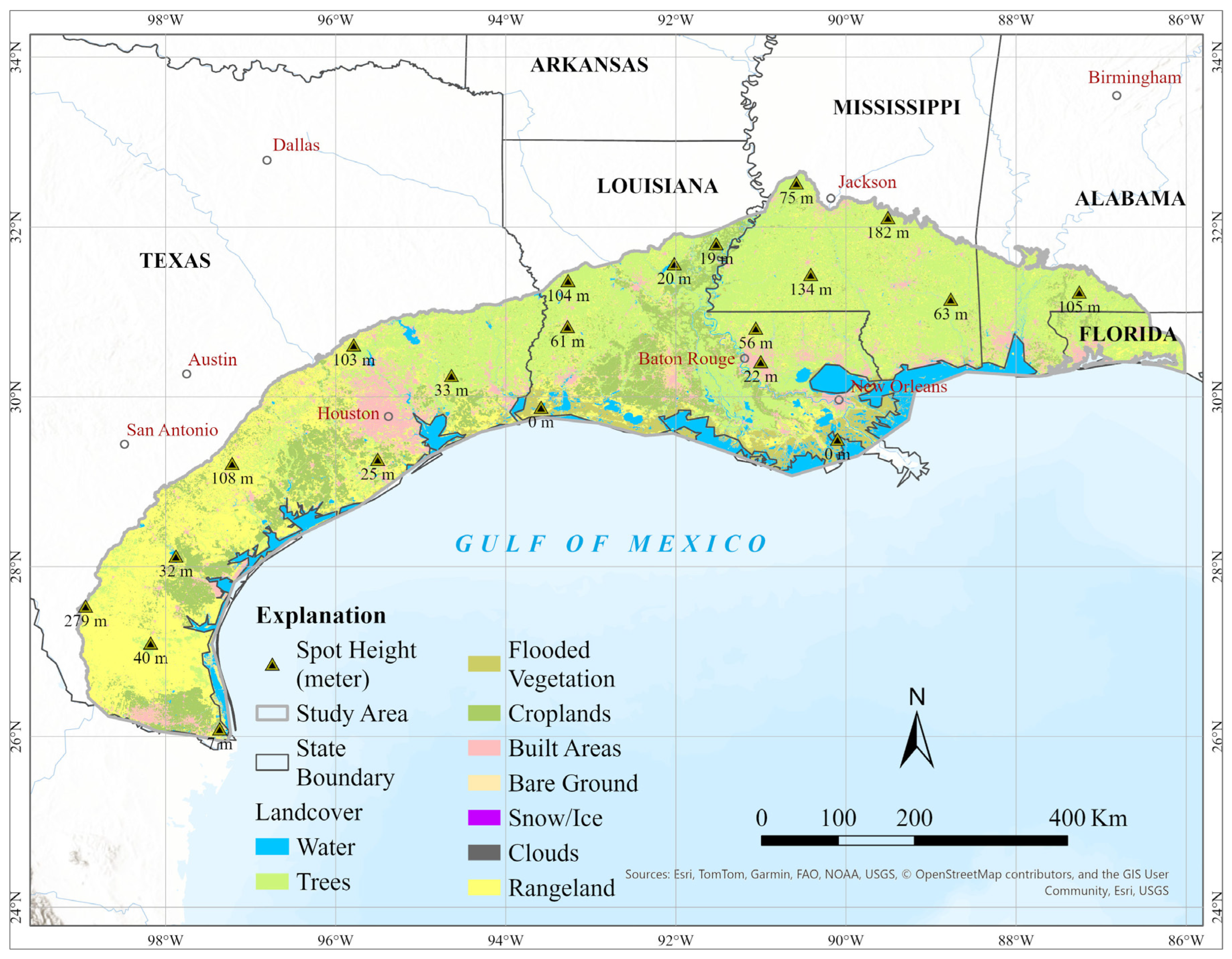
Figure 1. Location map of the study area (land cover data source: [21]).
Remotesensing 18 01680 g001
Figure 2. Generalized geohydrologic section showing zonation of the CLAS and regional groundwater flow direction [23].
Remotesensing 18 01680 g002
Figure 3. Process flow of the research.
Remotesensing 18 01680 g003
Figure 4. Histogram of R2 value of the downscaled monthly GRACE/GRACE-FO by (a) RF; (b) ANN; (c) DNN Model.
Remotesensing 18 01680 g004
Figure 5. Summary of rank of importance of the variables by ANN model.
Remotesensing 18 01680 g005
Figure 6. Monthly mean EWH: GRACE vs. downscaled ML models.
Remotesensing 18 01680 g006
Figure 7. Visual comparison of original GRACE data and model outputs for September 2015.
Remotesensing 18 01680 g007
Figure 8. Visual comparison of original GRACE data and model outputs for February 2023.
Remotesensing 18 01680 g008
Figure 9. Groundwater level monitoring wells of the study area.
Remotesensing 18 01680 g009
Figure 10. Spatial distribution of yearly mean. (a) Original GRACE TWSA, (b) ANN-based downscaled TWSA, and (c) GWLA distribution (2003–2023) of the study area. The red dashed line represents the temporal trend during the study period.
Remotesensing 18 01680 g010
Figure 11. Monthly mean (a) original GRACE TWSA (2003–2010); (b) original GRACE TWSA (2011–2016); (c) original GRACE TWSA (2019–2023); (d) downscaled TWSA (2003–2010); (e) downscaled TWSA (2011–2016); (f) downscaled TWSA (2019–2023); (g) ATM (2003–2010); (h) ATM (2011–2016); (i) ATM (2019–2023); (j) APT (2003–2010); (k) APT (2011–2016); (l) APT (2019–2023); (m) ANDVI (2003–2010); (n) ANDVI (2011–2016); (o) ANDVI (2019–2023); (p) AET (2003–2010); (q) AET (2011–2016); (r) AET (2019–2023) distribution of the study area. The red dashed line represents the temporal trend during the study period.
Remotesensing 18 01680 g011
Figure 12. Comparison of spatial resolution of (a) original GRACE-FO; (b) downscaled GRACE-FO (4 km × 4 km) from a previous study [61]; (c) downscaled GRACE-FO (800 m × 800 m) from January 2022 of the study area. The black box highlights the area used to compare how the spatial detail of TWS distribution changes with different spatial resolutions.
Remotesensing 18 01680 g012
Figure 13. Annual mean downscaled TWSA (2003–2023) for the Gulf Coast states.
Remotesensing 18 01680 g013
Figure 14. Scatter plot comparison of GRACE vs. downscaled TWSA (ANN).
Remotesensing 18 01680 g014
Figure 15. Comparison of TWS stress maps (2003–2023): (a) original GRACE TWSA and (b) ANN-based downscaled TWSA.
Remotesensing 18 01680 g015
Figure 16. TWS stress zones with Houston–Galveston subsidence AOI overlay.
Remotesensing 18 01680 g016
Table 1. Variables and their spatial resolutions.
VariablesSourceSpatial Resolution
GRACE/GRACE-FOJPL~111 km (Represent the ~300–330 km)
Mean TemperaturePRISM800 m
Total PrecipitationPRISM800 m
NDVIMODIS500 m
ETMODIS500 m
DEMSRTM30 m
Slope (Generated from DEM)SRTM30 m
Soil TypeFAO/UNESCOVector data
LithologyEsri250 m
Ground-based measurementUSGS/TWDB/MSDEQ/GSAL/FLDEPGroundwater table point data
Table 2. Error metrics of the model.
ModelR2RMSE
RF0.689–0.9930.002–0.027
ANN0.869–0.9890.002–0.019
DNN0.901–0.9920.001–0.016
Table 3. Spatial evaluation metrics of the models.
ModelMean Spatial Pearson rSD Spatial Pearson rMean SSIMSD SSIM
RF0.95380.03470.90480.0663
ANN0.96550.02040.91420.0803
DNN0.97600.01480.92000.0549
Table 4. Different zones of the TWS stress map (2003–2023) of the study area.
ZoneMean TWSA
(cm)
Condition
(Baseline)
Rate (cm/Year)95% CI of Rate
(± cm/Year)
Volume Change (Approx.)
(107 m3/Year)
Remark
Zone 1−2.00Deficit−0.30 ±0.25−10.70Depletion
Zone 2−1.15Deficit−0.17 ±0.24−15.00Depletion
Zone 3+0.33Above baseline+0.05 ±0.20+1.82Gain (not
significant)
Zone 4+1.41Above baseline+0.18 ±0.34+17.10Gain (not
significant)
Disclaimer/Publisher’s Note: The statements, opinions and data contained in all publications are solely those of the individual author(s) and contributor(s) and not of MDPI and/or the editor(s). MDPI and/or the editor(s) disclaim responsibility for any injury to people or property resulting from any ideas, methods, instructions or products referred to in the content.