A Spatial-Temporal Attention-Based U-Net for Crop Mapping from Time-Series Sentinel-2 Imagery: A Case in Sanjiang Plain

Highlights

What are the main findings?

• The proposed STA-UNet model achieves 93.61% overall accuracy and 0.925 F1-score for rice, maize, and soybean classification on the Sanjiang Plain using time-series Sentinel-2 imagery, outperforming state-of-the-art methods.
• STA-UNet achieves strong spatial transfer in the balanced left-subregion benchmark (OA of 85.02–87.53%), remains competitive in the rice-dominated right-subregion stress test, and demonstrates stable temporal generalization with limited inter-annual performance degradation.

What are the implications of the main findings?

• STA-UNet provides a robust and transferable framework for accurate crop mapping in cloud-prone, phenologically complex agricultural regions, supporting large-scale food security monitoring.
• The integration of spatial attention, temporal encoding, and adaptive feature fusion offers an effective strategy to overcome cloud interference and spatial heterogeneity challenges common in satellite-based crop classification.

Abstract

Food security is a growing global concern, and accurate crop mapping in major grain-producing regions like China’s Sanjiang Plain—which contributes approximately 7% of national grain output—is essential for agricultural resource management. However, crop classification in this area is hindered by frequent cloud cover, complex phenological rhythms, and spatial heterogeneity. To address these challenges, this study proposes Spatial-Temporal Attention U-Net (STA-UNet), a crop classification model based on time-series Sentinel-2 imagery, incorporating four key modules: Convolutional Block Attention for enhanced sensitivity to parcel boundaries, Temporal Attention Encoder for adaptive capture of temporal dependencies under cloud interference, Dynamic Upsampling for improved boundary recovery of small parcels, and Adaptive Feature Fusion for bridging semantic gaps between heterogeneous features. Extensive experiments on rice, maize, and soybean classification demonstrate that STA-UNet achieves an overall accuracy of 93.61% and an F1-score of 0.925, outperforming state-of-the-art methods. In spatial generalization tests, STA-UNet maintains overall accuracy above 85.02% in the left-subregion transfer setting and achieves the best three-year average OA of 81.34% in the rice-dominated right-subregion stress test, while temporal generalization tests confirm limited inter-annual performance degradation. These results indicate that STA-UNet provides a robust and effective framework for crop mapping in cloud-prone, phenologically complex agricultural regions.

1. Introduction

The global challenges to food security are escalating due to sustained population growth, an increase in the frequency of extreme climate events, a reduction in arable land, and rising geopolitical tensions. The 2030 Agenda for Sustainable Development explicitly outlines objectives aimed at eradicating hunger, achieving food security, enhancing nutrition, and promoting sustainable agricultural practices. Concurrently, the World Food Security Summit report titled “How to Feed the World in 2050” anticipates that global food production must increase by approximately 70% by the year 2050 to cater to the needs of an estimated population of 9.1 billion people. In light of these circumstances, harnessing remote sensing technology for precision agricultural management is essential for enhancing productivity while operating within resource constraints [1]. Therefore, timely and precise information regarding large-scale crop distribution is vital for assessing food security and optimizing the allocation of agricultural resources; this forms a fundamental basis for national food security strategies [2].

Traditional field-survey-based crop mapping provides reliable reference data; however, it is hindered by high costs, limited timeliness, and restricted spatial coverage. These constraints render it inadequate for operational large-area monitoring [3,4]. With the rapid advancements in Earth observation technologies, large-scale crop identification and mapping utilizing multi-temporal remote sensing imagery have emerged as a predominant approach [5,6,7,8]. Multi-temporal datasets capture spectral dynamics throughout the entire phenological cycle, thereby yielding rich spatial-temporal information essential for accurate crop classification [9,10]. Nevertheless, classification efforts continue to face challenges due to temporal data gaps (e.g., those caused by cloud cover), significant phenological variability, and ambiguous parcel boundaries [11].

To address these challenges, a range of crop classification approaches has been developed, encompassing traditional techniques, machine learning approaches, and deep learning algorithms. Early pixel-based traditional classifiers, such as the maximum likelihood classifier, are characterized by their computational efficiency; however, they exhibit high sensitivity to noise and show limited accuracy. These methods perform poorly in complex agricultural landscapes and struggle to account for spatial-temporal variability. Following this, advancements in machine learning have led to the widespread adoption of classifiers like support vector machines and random forests [12,13]. By constructing nonlinear decision boundaries, these methodologies enhance the classification accuracy; however, they lack the capacity for automatic feature learning. As a result, they fail to fully exploit the temporal characteristics inherent in multi-temporal remote sensing data [14,15].

Over the past decade, the widespread utilization of deep learning techniques in remote sensing has opened new pathways for crop classification [16,17,18,19,20]. Convolutional neural networks (CNNs) excel at automatic feature extraction and spatial pattern recognition, effectively learning spectral-spatial representations and demonstrating significant advantages in fine-scale crop-type mapping [21,22,23,24,25]. However, these networks primarily focus on spatial and spectral dimensions and have a limited capability to model long-term temporal dependencies. Additionally, they lack mechanisms for multi-scale feature fusion, leading to noticeable performance degradation when addressing complex field boundaries [26,27,28]. Graph neural networks (GNNs) can adeptly model spatial adjacency relationships and topological structures among farmland parcels [29,30]. Nonetheless, they depend on predefined graph structures and neighborhoods. When applied to expansive continuous agricultural regions, GNNs incur high computational complexity and encounter challenges in balancing pixel-level fine-grained classification with region-level semantic understanding [31,32,33,34]. Attention mechanisms offer the advantage of adaptively focusing on critical temporal information and salient spatial regions, thereby enhancing sensitivity to pivotal phenological stages [35,36,37,38]. However, when employed independently, these mechanisms fall short of providing an effective spatial reconstruction method for boundary detail recovery. Moreover, their substantial computational overhead limits efficiency in large-scale applications [39,40,41].

Owing to the encoder–decoder design and skip connections, U-Net architectures have demonstrated exceptional performance in the semantic segmentation of remote sensing imagery [42,43,44]. To address the limitations associated with conventional deep learning methods in harnessing temporal information and preserving boundary details, researchers have integrated U-Net with time-series processing strategies, proposing three primary avenues for enhancement: the 3D convolutional approach based on U-Net architecture integrates temporal dimensions into its encoder–decoder structure, preserving detailed sequential characteristics through skip connections while effectively capturing temporal, spatial, and spectral features [45,46,47]; the hybrid U-Net with recurrent neural networks incorporates LSTM or GRU modules within the encoder to process temporal dependencies, leveraging U-Net’s skip connection mechanism to mitigate gradient vanishing issues [48,49,50]; by integrating temporal and spatial attention mechanisms into conventional U-Net architecture, an end-to-end spatiotemporal feature extraction framework is established, achieving optimal balance between classification accuracy and computational efficiency [51,52,53].

Recent crop-mapping studies have increasingly emphasized the transferability of models across regions and years using satellite-based time-series data. Because ground-truth crop labels are often unavailable—or prohibitively costly to acquire—in target regions or seasons, transfer-learning approaches aim to leverage labeled source-domain data and adapt learned spectral-temporal representations to new domains. Early transfer-learning efforts trained classifiers using high-confidence samples from the Cropland Data Layer (CDL) and harmonized Landsat–Sentinel NDVI time series. These studies demonstrate that crop phenological trajectories encode transferable information across geographic regions, although robust cross-region transfer typically requires sufficiently long growing-season observations [54]. Subsequent inter-annual transfer studies further show that classifiers trained on one year can be successfully transferred to unseen target years—even in the absence of contemporaneous crop reference labels—provided that multi-temporal Sentinel-2 observations deliver stable phenological and spectral signatures [55]. More recent deep learning approaches have advanced cross-domain crop mapping through temporal alignment, fine-tuning, and domain-adaptation strategies: TimeMatch explicitly estimates unsupervised phenological time shifts to enable cross-region adaptation from satellite image time series [56]; Transformer-based transfer learning adapts Sentinel-2 time-series representations across distinct agricultural regions [57]; and temporal encoding coupled with augmentation techniques allows deep models trained on single-year reference data to generalize effectively across extended multi-year Landsat–Sentinel time series [58]. In addition, a novel Contrastive Self-Training Network (CSTN) synergistically integrates self-training with contrastive domain adaptation to improve cross-regional crop mapping from satellite imagery time series [59]. Nevertheless, these studies also reveal that domain shift—arising from regional differences in crop calendars, inter-annual climate variability, irregular clear-sky observation availability, and scarcity of labeled target-domain samples—remains a critical bottleneck. Consequently, for pixel-level crop mapping in cloud-prone agricultural regions, transferability must be jointly optimized with robust temporal feature extraction and accurate parcel-boundary reconstruction.

Despite notable advancements, three critical challenges continue to hinder crop classification using time-series remote sensing: cloud cover phenomena lead to discontinuities and data gaps in time-series remote sensing data, which significantly impair the model’s ability to accurately capture crop phenological characteristics and degrade its overall performance; prevailing deep learning methodologies typically necessitate intricate data preprocessing procedures and specialized technical expertise, resulting in high deployment barriers for practical agricultural applications and consequently limiting their widespread adoption; research on cropland classification under specific geographic and climatic conditions—such as complex terrain and rapidly changing phenological traits—remains relatively insufficient.

In response to the aforementioned key challenges, this study introduces Spatial-Temporal Attention U-Net (STA-UNet), a deep learning architecture based on the U-Net framework that incorporates dual spatial-temporal attention. This approach alleviates information loss during upsampling and facilitates Adaptive Feature Fusion. By leveraging multi-temporal remote sensing imagery, the network combines a Convolutional Block Attention (CBA) module, a Temporal Attention Encoder (TAE) module, a Dynamic Upsampling (DU) module, and an Adaptive Feature Fusion (AFF) module to enable precise crop classification in complex environments. Notably, STA-UNet effectively suppresses temporal noise induced by cloud cover without relying on cloud-detection preprocessing while accurately capturing rapid phenological dynamics associated with high-latitude regions of the Sanjiang Plain alongside intricate spatial patterns of farmland parcels.

The main contributions of this article are as follows:

• By utilizing long-time series data from Sentinel-2, a crop classification dataset covering the Sanjiang Plain is constructed. This dataset incorporates multi-temporal observations under complex weather conditions, thereby providing a robust data foundation for research in crop mapping.
• To address regional characteristics such as frequent cloud cover, pronounced phenological heterogeneity, and complex field patterns, an STA-UNet is proposed that achieves high-accuracy crop classification without cloud-detection preprocessing.
• A series of comprehensive comparative and ablation experiments has been meticulously designed to validate the advantages of STA-UNet over existing mainstream models with respect to classification accuracy.
• Spatial and temporal generalization experiments are conducted to evaluate cross-region and cross-year applicability, thereby providing reliable methodological support for large-scale crop mapping in the Sanjiang Plain.

The remainder of this paper is organized as follows: Section 2 provides a detailed overview of the study area and dataset. Section 3 elaborates on the network architecture of STA-UNet and elucidates the operational principles of its constituent modules. The experimental settings and evaluation metrics are described in Section 4. Section 5 reports the results of comparative and ablation experiments as well as spatial and temporal generalization experiments. Section 6 discusses the findings, and Section 7 concludes the paper.

2. Study Area and Dataset

2.1. Study Area

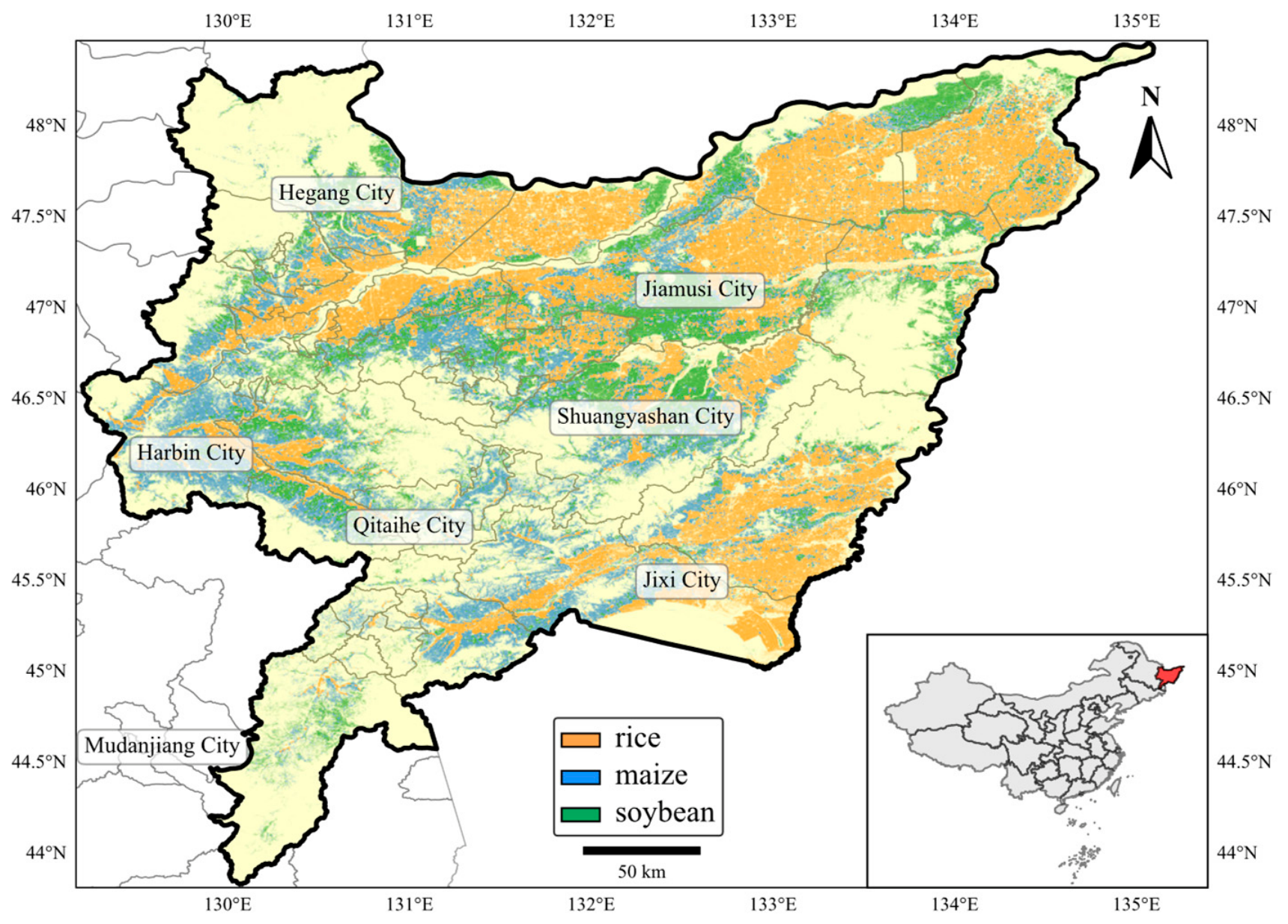
The Sanjiang Plain, located in Heilongjiang Province of Northeast China, has been selected as the study area, as depicted in Figure 1. This region occupies the northeastern Heilongjiang (43.48–48.23°N, 129.1–135.0°E) and spans approximately 54,000 km², making it one of China’s major grain-producing areas. The mean annual temperature of the region ranges from 2.5 °C to 4.0 °C, with annual precipitation averaging between 500 mm and 600 mm; notably, around 80% of this precipitation occurs between June and September. Such climatic conditions support a typical single-cropping system characterized by a short growing season and rapid phenological progression. The latitude span of approximately 5° leads to significant variation in solar radiation across the Plain, causing pronounced north–south differences in crop phenological rhythms—a factor that complicates remote sensing monitoring efforts. The dominant crops cultivated within the region include rice, maize, and soybean: rice is primarily grown in low-lying areas with abundant water resources; maize thrives mainly on well-drained plains and gentle hills; and soybean is widely distributed throughout various landscapes across the region.

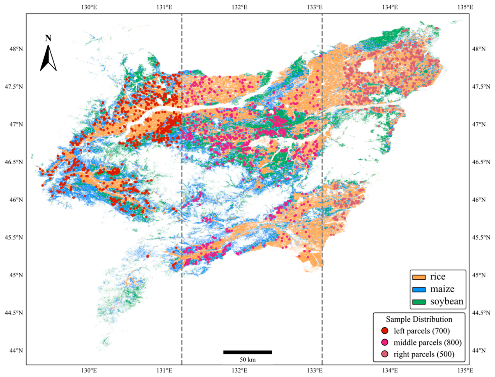
To systematically evaluate spatial generalization, the study area is longitudinally partitioned into three subregions: left, middle, and right. This division is informed by variations in topography, hydrological networks, and agricultural management practices, as illustrated in Figure 2. The left subregion is characterized by relatively elevated terrain and a higher proportion of maize cultivation; the middle subregion, located at the core of Sanjiang Plain, exhibits optimal agricultural conditions with a balanced distribution of all three crops; conversely, the right subregion lies adjacent to the Ussuri River and benefits from abundant water resources along with a predominance of rice production. For model training, validation, and testing purposes, 800 parcels are selected from the middle subregion based on criteria of data quality, typicality, and representativeness. Meanwhile, 700 parcels from the left subregion are utilized to assess spatial generalization, and 500 parcels from the right subregion are further included as an additional rice-dominated stress-test set.

2.2. Dataset

2.2.1. Crop Labels

The remote sensing monitoring dataset of primary crop planting distributions in the Sanjiang Plain from 2020 to 2022 serves as the source for crop labels. This classification dataset is developed utilizing time-series imagery from Sentinel-2 satellites, alongside field surveys of representative land-cover types within the Sanjiang Plain. Key spectral bands associated with major crops and their typical surrounding elements are selected, after which a random forest classifier is employed to delineate the planting distributions of the three principal crops—rice, maize, and soybean—for the years 2020 through 2022. Validated against the field-survey data, the overall accuracies achieved for 2020, 2021, and 2022 are recorded at 95.18%, 95.0%, and 94.5%, respectively; Kappa coefficients are calculated at values of 0.924, 0.925, and 0.919 for these years, respectively, indicating a high degree of reliability. These labels form the foundation for subsequent dataset construction as well as model training and testing.

2.2.2. Satellite Data

The primary data source for this study is the Sentinel-2 multispectral imagery provided by the European Space Agency (ESA). The Sentinel-2 satellite is equipped with the Multispectral Instrument (MSI), which captures spectral information of the Earth’s surface at multiple spatial resolutions of 10 m, 20 m, and 60 m [60]. The Sentinel-2 constellation comprises two platforms, namely 2A and 2B, orbiting at an altitude of 786 km. With a combined revisit time of 5 days and a swath width of approximately 290 km, it is particularly well-suited for monitoring large-scale agricultural areas. In order to fulfill crop classification demands and ensure data quality, ten specific bands from Sentinel-2 have been selected. These encompass three visible bands at a resolution of 10 m—namely B2 (blue), B3 (green), and B4 (red)—as well as one near-infrared band (B8). Additionally, the selected bands include red-edge bands captured at a resolution of 20 m (B5, B6, B7), along with a narrow near-infrared band (B8A) and two shortwave infrared bands (B11 and B12). Collectively, these bands effectively capture spectral signatures throughout the vegetation growth cycle; in particular, the red-edge bands exhibit heightened sensitivity to vegetation status and yield critical insights into phenological dynamics. This study utilizes Level-2A (L2A) surface reflectance products derived from Sentinel-2 data that have undergone atmospheric correction.

Satellite data acquisition encompasses the calendar years 2020, 2021, and 2022. Due to its high-latitude location, the Sanjiang Plain is frequently subjected to cloud cover, which limits the availability of valid observations. An initial screening process employed a threshold of 60% cloud cover. For each parcel analyzed, the annual number of Sentinel-2 acquisitions varies from 9 to 94, with an average of approximately 66 images per year. The imagery is sourced via the Copernicus Open Access Hub (https://www.copernicus.eu/en/access-data, accessed on 20 May 2026).

2.2.3. Data Preprocessing

The data preprocessing pipeline consists of four primary steps:

• Sample selection: Crop labels are initially obtained for the Sanjiang Plain. The label map is divided into parcels measuring 128 × 128 pixels, with those exhibiting a non-cropland proportion below 25% being retained to ensure that cropland signals predominantly prevail. This procedure yields over 20,000 parcels per year.
• Image acquisition and preprocessing: Sentinel-2 images with scene-level cloud cover of less than 60% are obtained for the study area. The original SAFE packages are transformed into GeoTIFF format. For the bands at a resolution of 20 m (B5, B6, B7, B8A, B11, and B12), bilinear interpolation is employed to resample these bands to a unified resolution of 10 m across all bands.
• Time-series construction: In instances where multiple Sentinel-2 images overlap a specific parcel on the same date, one image is selected based on a weighted combination of valid pixel ratio, data variance, and brightness distribution for inclusion in that parcel’s time series. To address inconsistencies in sequence lengths among parcels while preserving all available annual observations, a year-specific fixed-length temporal window is adopted. After selecting one image for each parcel on each acquisition date, the maximum sequence lengths are 87, 99, and 95 observations for 2020, 2021, and 2022, respectively; these values are therefore used as the temporal window lengths for the corresponding years. Parcels with fewer observations are zero-padded to the annual window length, and a binary padding mask is used to ensure that padded time steps do not contribute to temporal feature aggregation. The same windowing and masking strategy is applied during training, validation, testing, and generalization experiments. This design considers two factors: first, real-world applications seldom guarantee perfectly preprocessed inputs; therefore, it is critical to assess the network’s ability to adapt to raw data, particularly regarding whether spatial-temporal attention can effectively learn significant temporal features without dependence on cloud preprocessing; second, under multi-temporal conditions, the network is anticipated to identify stable spectral-temporal patterns that mitigate sensitivity towards the quality of individual acquisition events.
• Temporal coverage checking: To verify that the selected reference samples are supported by full-growing-season observations, the acquisition dates recorded in the metadata file of each patch are examined. Three phenological windows are considered according to the single-cropping calendar of the Sanjiang Plain: planting/green-up (May–June), peak growth (July–August), and senescence/harvest (September–October). For the middle- and left-subregion sets, all selected patches in 2020 and 2021 contain observations in all three windows, while the corresponding coverage rates in 2022 are 98.1% and 99.3% for the middle and left sets, respectively. For the right-subregion set, the coverage rates are 100%, 100%, and 95.6% for 2020, 2021, and 2022, respectively. This check confirms that the samples used for training and evaluation are associated with multi-temporal observations spanning the major crop growth stages.
• Dataset and generalization splits: Based on the distributions of parcels across the three subregions, the left subregion contains approximately 6000 parcels; the middle one consists of around 10,000 valid parcels; and the right subregion has about 5000 parcels. All candidate parcels are first subjected to the same non-cropland filtering and temporal-coverage checking procedures; no additional manual visual screening is used to select only cleaner or easier samples. From these candidate pools, stratified random sampling is implemented to select 800 parcels from the middle subregion for the standard dataset and 700 parcels from the left subregion for the main spatial generalization test. The purpose of this sampling is to construct controlled and comparable benchmark subsets with similar class balance and sufficient temporal coverage. To further evaluate model robustness under realistic class imbalance, 500 parcels from the right subregion are also selected as an additional spatial generalization set. Crop-type distributions by year and subregions are summarized in

  Table 1. Pixel-level class ratios of the selected left-, middle-, and right-subregion sample sets (%).

  Year	Subregion	Background	Rice	Maize	Soybean
  2020	Left	18.23	30.33	30.61	20.83
  	Middle	14.59	32.71	28.86	23.84
  	Right	14.76	79.22	1.53	4.50
  2021	Left	17.83	30.14	31.34	20.69
  	Middle	17.44	30.90	29.89	21.77
  	Right	15.15	70.18	7.73	6.95
  2022	Left	18.08	27.91	29.16	24.85
  	Middle	16.48	30.41	29.94	23.17
  	Right	13.70	68.75	11.59	5.96

  .

2.3. Training/Testing Datasets

To comprehensively evaluate the applicability and stability of the model, three distinct evaluation schemes are designed: a standard test, a spatial generalization test, and a temporal generalization test.

• Standard Test: The dataset consists of 800 parcels sourced from the middle subregion and is randomly divided into training (70%; 560 parcels), validation (15%; 120 parcels), and test (15%; 120 parcels) sets. This random sampling method ensures that no set is influenced by extraneous factors. The training set is utilized for parameter optimization, the validation set is employed for hyperparameter tuning and overfitting prevention, while the test set serves to assess the performance on unseen data.
• Spatial Generalization Test: Two spatial generalization sets are constructed to evaluate model transfer across regional differences. The first set consists of 700 selected parcels from the left subregion and is used as the main cross-region benchmark because it retains relatively balanced crop distributions comparable to the middle-subregion standard dataset. The second set consists of 500 selected parcels from the right subregion and is used as an additional imbalanced stress test because it is dominated by rice and contains substantially fewer maize and soybean pixels. Together, these two settings evaluate the model’s ability to handle both spatial heterogeneity and realistic class imbalance.
• Temporal Generalization Test: A cross-year evaluation strategy is implemented to examine the generalization across different years. Six combinations are evaluated: models trained on the dataset from 2020 are tested against the data from 2021 and 2022; models trained on the dataset from 2021 are evaluated with respect to the data from 2020 and 2022; and models trained on the dataset from 2022 are tested using the information from both 2020 and 2021. This comprehensive approach assesses the model’s robustness to inter-annual climate fluctuations, phenological variations, and changes in agricultural management practices.

3. Methodology

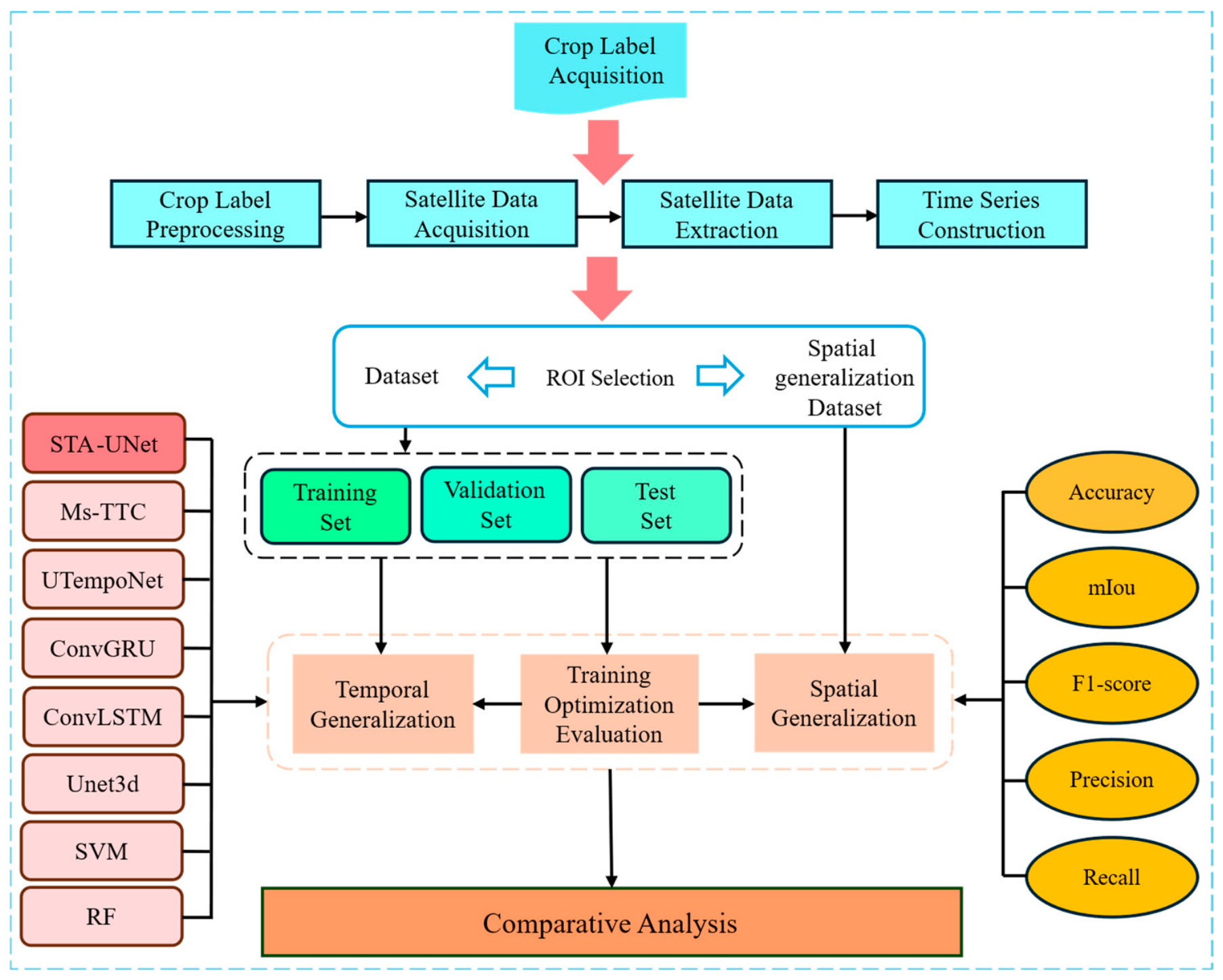
The proposed STA-UNet aims to tackle three primary challenges that affect classification accuracy in the Sanjiang Plain: temporal discontinuities caused by cloud cover, regional phenological variations resulting from spatial heterogeneity, and the meticulous representation of intricate field structures. The overall workflow is illustrated in Figure 3: initially, data preprocessing is conducted to construct both the main dataset and the spatial generalization set; subsequently, standard tests as well as spatial and temporal generalization tests are conducted, comparing STA-UNet against seven state-of-the-art (SOTA) methods (Ms-TTC [61], UTempoNet [49], ConvGRU [48], ConvLSTM [50], Unet3d [62], support vector machine (SVM) [63], and random forest (RF) [64]); finally, a comprehensive analysis and summary of the experimental results are provided.

3.1. Model Overview

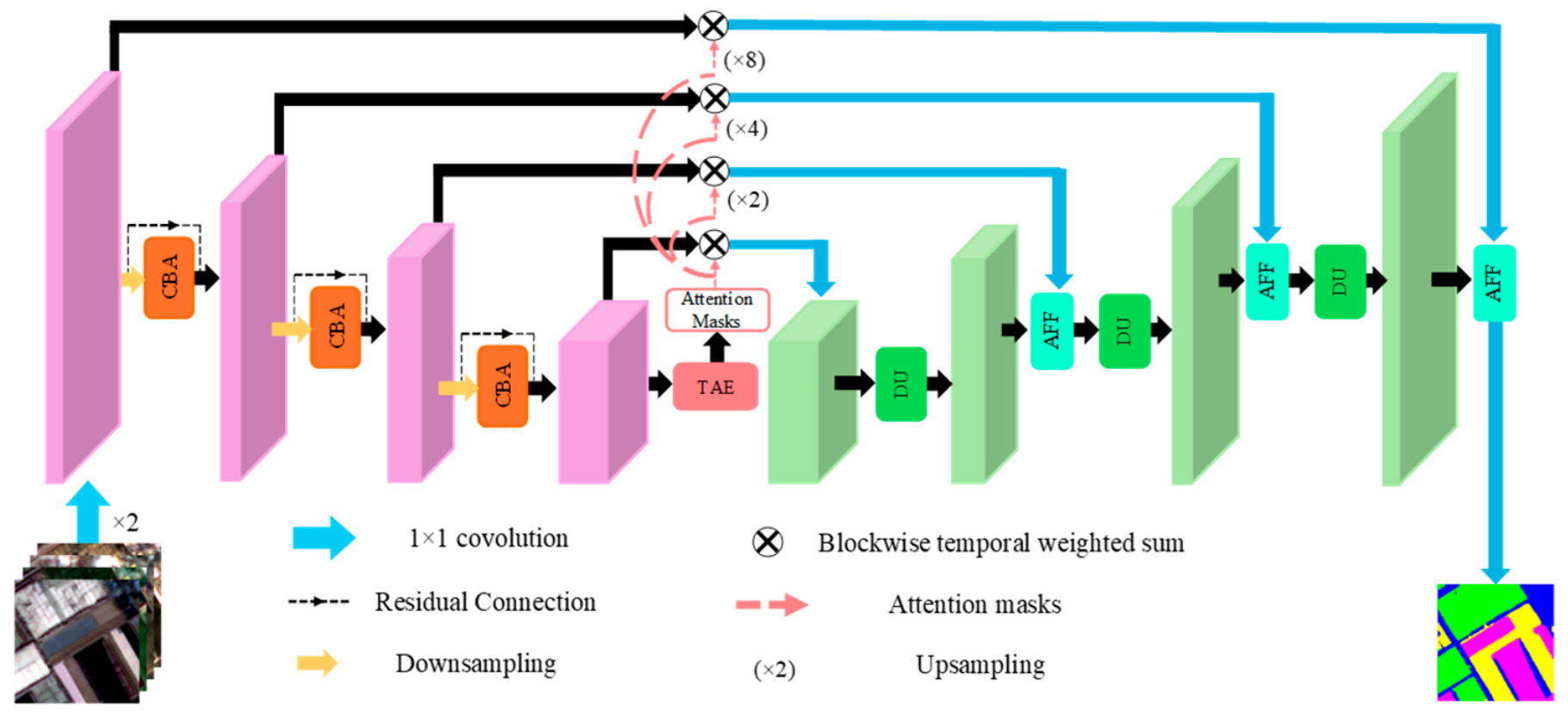
STA-UNet is designed as a phenology-guided and boundary-aware spatial-temporal U-Net for crop mapping from irregular Sentinel-2 time series, as depicted in Figure 4. Its methodological design follows a coordinated encoder–temporal–decoder pathway. First, channel-spatial attention is embedded in the encoder to enhance crop-related spectral-spatial responses and suppress redundant background or mixed-boundary features before temporal aggregation. Second, a Temporal Attention Encoder assigns adaptive weights to multi-date observations and uses padding masks to reduce the influence of missing or cloud-contaminated acquisitions, enabling the model to focus on discriminative phenological stages of rice, maize, and soybean. Third, the learned temporal attention weights are propagated to multi-scale skip features, allowing temporal cues extracted at deep layers to guide high-resolution spatial reconstruction. Finally, Dynamic Upsampling and Adaptive Feature Fusion are coupled in the decoder so that learned sampling offsets recover fine parcel boundaries while similarity-guided fusion reduces semantic inconsistency between encoder and decoder features.

The network utilizes multi-temporal Sentinel-2 images as its input. Initially, it performs two convolutional layers for shallow feature extraction, followed by a series of downsampling operations. At the lowest resolution level, temporal attention mechanisms are implemented. Subsequently, progressive upsampling is conducted to recover spatial details; during this phase, features from skip connections are fused with those being upsampled. Finally, a classifier yields both a per-pixel land-cover probability map and the final classification map.

3.2. Key Components

3.2.1. Convolutional Block Attention (CBA) Module

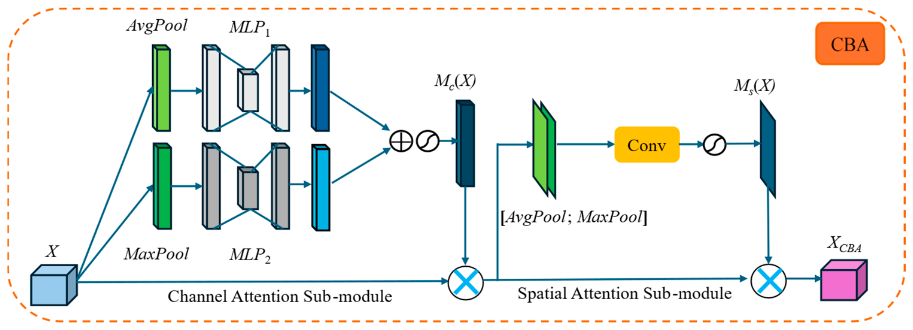
The CBA module is used as an encoder-side spatial-spectral refinement unit after each strided downsampling block, as depicted in Figure 5. For multi-temporal Sentinel-2 inputs, the convolutional encoder extracts features from each observation, and CBA further recalibrates these features before temporal aggregation. Given the downsampled feature map at a specific scale, CBA first estimates channel-wise importance to emphasize crop-related spectral responses, and then estimates spatial importance to highlight parcel interiors and boundary-sensitive regions. The refined response is added back to the downsampled feature through a residual connection, so the encoder preserves the original convolutional representation while enhancing discriminative spatial-spectral cues.

For channel recalibration, the downsampled feature map X is compressed along the spatial dimensions using global average pooling and global max pooling. The two descriptors summarize complementary spectral-spatial responses of the current observation and are passed through multilayer projections. Their outputs are added and activated by a sigmoid function to produce the channel attention map M_c(X), as expressed in (1):

$$M_c(X)=\sigma (ML{P}_1(AvgPool(X))+ML{P}_2(MaxPool(X)))$$

(1)

where X denotes the downsampled time-series feature map, σ represents the sigmoid function, and MLP₁(·) and MLP₂(·) refer to distinct multilayer perceptrons.

After channel recalibration, spatial attention is computed from the channel-refined feature. Specifically, average pooling and max pooling are applied along the channel dimension and concatenated to form a two-channel spatial descriptor. A 7 × 7 convolution followed by a sigmoid function then generates the spatial attention map M_s(X), as expressed in (2):

$$M_s(X)=\sigma (Con{v}_{7\times 7}([AvgPool(X\odot M_c(X));MaxPool(X\odot M_c(X))]))$$

(2)

where Conv_7×7 is the 7 × 7 convolution, $\odot$ denotes the element-wise multiplication with channel broadcasting.

The CBA-refined feature is obtained by sequentially applying channel and spatial attention to X. In the encoder block, this refined feature is further combined with the original downsampled feature through residual addition, producing the output feature X_CBA for subsequent temporal encoding:

$$X_{CBA}=X+\left(X\odot M_c(X)\odot M_s(X)\right)$$

(3)

3.2.2. Temporal Attention Encoder (TAE) Module

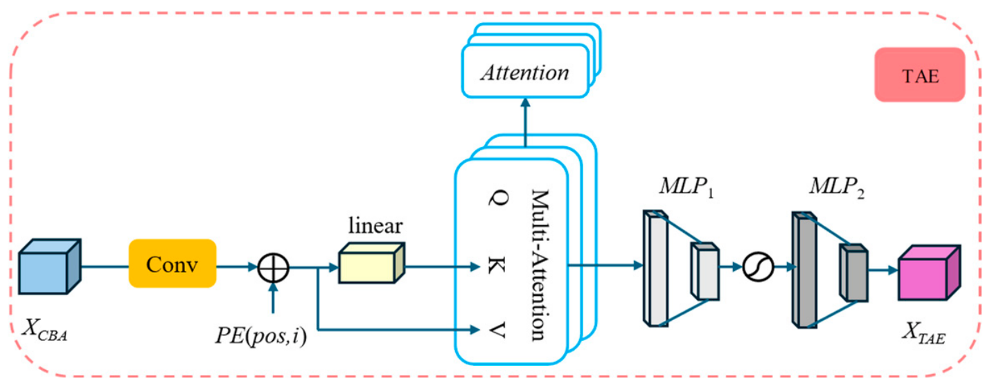
The TAE module performs phenology-aware temporal encoding on the CBA-refined multi-temporal features, as shown in Figure 6. After the encoder has enhanced spatial-spectral responses at each observation date, TAE aggregates the temporal dimension by learning date-specific attention weights for each spatial location. This design allows STA-UNet to convert irregular Sentinel-2 observations into a compact feature representation while retaining the key phenological cues required for distinguishing rice, maize, and soybean.

The processing pipeline is as follows: initially, X_CBA is subjected to pointwise convolution and Group Normalization to yield X_d; subsequently, sinusoidal positional encoding is incorporated to obtain the position-embedded time-series feature map X_pos. The calculation for this encoding can be expressed by the formula:

$$X_{pos}=X_d+PE(pos,i)$$

(4)

$$PE(pos,i)=\left\{\begin{array}{ll}\sin \left({\displaystyle \frac{pos}{{1000}^{2k/d_m}}}\right),\hfill & if i=2k\hfill \\ \cos \left({\displaystyle \frac{pos}{{1000}^{2k/d_m}}}\right),\hfill & if i=2k+1\hfill \end{array}\right.$$

(5)

where PE(pos, i) denotes the positional encoding function, pos represents the temporal index, i signifies the channel index, and d_m indicates the feature dimension. k is a natural number and satisfies $0\le k<d_m/2$.

Temporal attention is computed using a multi-head attention mechanism with learnable query vectors. For each attention head, the query Q (Query) is learned as a temporal pattern prototype, the key K (Key) is generated from X_pos through a linear projection, and the value V (Value) is obtained by splitting the projected temporal feature into head-specific channel groups. The scaled dot-product between Q and K produces an attention weight over the observation dates for each pixel. When padded observations exist, the padding mask is applied before the softmax operation so that padded dates do not participate in temporal aggregation. The attention-weighted value features from all heads are then concatenated:

$$Attention=\mathrm{softmax}\left({\displaystyle \frac{Q_h{K}_h^T}{\sqrt{d_k}}}\right)$$

(6)

$$X_{attn}=Attention\cdot X_{pos}$$

(7)

where h denotes the number of heads, d_k is the queries and keys of dimension, and · is the element-wise multiplication.

The concatenated multi-head features are further processed by a multilayer perceptron and normalization layer to generate the temporally aggregated feature map X_TAE:

$$X_{TAE}=ML{P}_2\cdot ReLU(ML{P}_1\cdot X_{attn})$$

(8)

where ReLU(·) denotes the nonlinear activation function.

The learned temporal attention maps are further used to aggregate the multi-scale skip features from the encoder. For a skip feature sequence at a given encoder scale, the attention maps are resized to the corresponding spatial resolution by bilinear interpolation. In the grouped attention mode, the feature channels are divided according to the attention heads, and each channel group is weighted by the corresponding temporal attention map. The weighted features are summed along the temporal dimension and concatenated across heads to obtain the aggregated skip feature X_skip, as shown in (9). The same padding mask is applied during this process to exclude padded observations from the skip aggregation.

$$X_{skip}=Con{v}_{1\times 1}\left(Concat{\left[{\displaystyle \sum _{t=1}^{T}Attention}\odot X_{up}\right]}_{n=1}^h\right)$$

(9)

Through this two-stage use of temporal attention, TAE provides both a deep temporally aggregated representation and multi-scale attention-guided skip features. The deep representation summarizes crop phenological dynamics at the semantic level, while the skip aggregation transfers date-specific temporal cues back to higher-resolution decoder stages. As a result, the decoder receives spatial details that have already been temporally filtered, which improves the stability of feature reconstruction under missing, irregular, or less informative observations.

3.2.3. Dynamic Upsampling (DU) Module

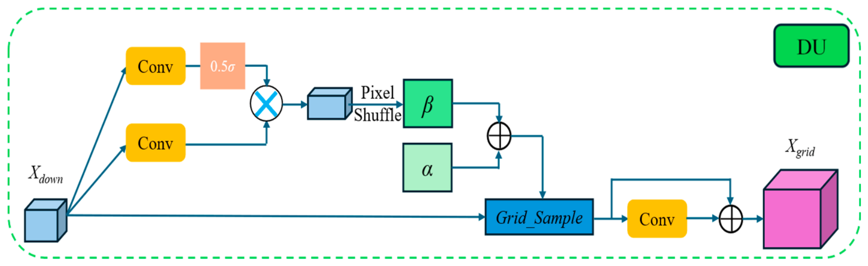
The DU module is used in each decoder stage to reconstruct high-resolution feature maps from low-resolution semantic features, as illustrated in Figure 7. In crop mapping, parcel boundaries and narrow background intervals can be weakened after repeated downsampling, making the decoder sensitive to the sampling positions used during feature recovery. DU addresses this issue by predicting content-dependent sampling offsets from the decoder feature itself. The module learns where each upsampled position should sample from the low-resolution feature space and then performs grid-based resampling to obtain boundary-aware decoder features.

Concretely, given the low-resolution decoder feature X_down, a 1 × 1 offset convolution predicts the sampling displacement for each upsampling group. In parallel, a scope convolution followed by a sigmoid function estimates a modulation factor that controls the range of the learned displacement. The predicted offset is multiplied by the scope factor and scaled by 0.5, and then added to the initialized regular sampling grid α to obtain the final sampling coordinate offset Δ. This process can be formulated as follows:

$$\Delta =PS(Con{v}_{offset}\left(X_{down}\right)\cdot \sigma \left(Con{v}_{scope}\left(X_{down}\right)\right)\cdot 0.5)+\alpha$$

(10)

where PS(·) denotes the pixel shuffle operation used to rearrange group-wise offsets to the upsampled resolution, Conv_offset(·) refers to the offset convolution, and Conv_scope(·) indicates the range-scaling convolution.

The process begins with grid sampling on X_down using bilinear interpolation in conjunction with Δ. This is followed by a post-processing convolution and the incorporation of a residual connection, resulting in the generation of the upsampled feature map X_grid.

3.2.4. Adaptive Feature Fusion (AFF) Module

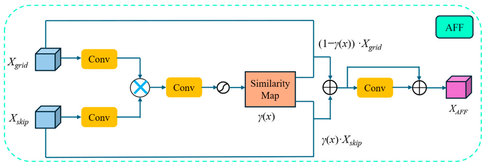
The AFF module is used after each DU operation to fuse the upsampled decoder feature with the temporally aggregated skip feature, as depicted in Figure 8. At this stage, the decoder feature contains high-level temporal semantics recovered from the bottleneck, whereas the skip feature preserves higher-resolution spatial details that have been filtered by TAE attention. AFF estimates their local correspondence and uses it to control how much skip information should be injected into the decoder representation.

Given the upsampled decoder feature X_grid and the aggregated skip feature X_skip, AFF first aligns their channel dimensions through pointwise projections. The two projected features are then compared at each spatial location to produce a similarity map, which serves as a soft gate for feature fusion. A larger similarity response indicates that the skip feature is more consistent with the current decoder representation and can therefore contribute more strongly to spatial detail recovery.

In detail, X_grid and X_skip are initially processed by pointwise convolutions to obtain intermediate feature maps X_G and X_S, respectively. These two maps are subsequently combined using element-wise multiplication with channel broadcasting, followed by convolution and application of a sigmoid function to generate a similarity map γ(x), upon which adaptive fusion occurs. Finally, a pointwise convolution coupled with a residual connection yields the AFF module output feature map X_AFF.

4. Experiments

4.1. Experimental Settings

STA-UNet is configured with encoder widths of [64, 64, 64, 128], decoder widths of [32, 64, 64, 128], and an output convolution layer of [32, 4], corresponding to background, rice, maize, and soybean. In the TAE module, the number of attention heads (h) is set to 16, the feature dimension (d_m) is 256, and the query/key dimension (d_k) is 4. The skip-connection aggregation uses a grouped head-wise weighting scheme. During downsampling, the convolution kernel size, stride, and padding are set to 4, 2, and 1, respectively. Group Normalization is adopted in the encoder to stabilize training under the small batch size used for time-series imagery.

STA-UNet’s performance is compared against five deep learning models (Ms-TTC, UTempoNet, ConvGRU, ConvLSTM, and Unet3d) and two classical machine learning baselines (SVM and RF).

Table 2. Parameter counts of different models.

Method	Number of Parameters
Ms-TTC	1,170,850
UTempoNet	1,180,416
ConvGRU	930,424
ConvLSTM	985,604
Unet3d	1,546,868
SVM	N/A
RF	N/A
STA-UNet	649,650

presents the parameter counts of different models. To ensure a fair comparison, all competing models use the same Sentinel-2 input data, including the same 10 spectral bands resampled to 10 m resolution, 128 × 128 image patches, crop-label maps, and training, validation, and test splits.

All deep learning models are trained for multi-class pixel-wise crop classification using cross-entropy loss, the Adam optimizer, an initial learning rate of 0.001, a weight decay of 5 × 10⁻⁴, a batch size of 4, and 80 epochs. Hyperparameters are selected based only on the validation set, and the test set is not used during model selection. Each experiment is repeated three times, and the reported values are the averages. Sentinel-2 reflectance values are normalized using pre-computed year-specific channel-wise means and standard deviations stored with each annual dataset. For each spectral band, the mean and standard deviation are computed from Sentinel-2 patches by aggregating over temporal observations and spatial pixels. The corresponding annual normalization statistics are applied consistently to all models and evaluation subsets from the same year. No additional data augmentation or early stopping is used.

For SVM and RF, the same preprocessed Sentinel-2 observations and crop-label maps are used. Each valid pixel is represented by concatenating all available temporal-band values and five per-band temporal statistics: mean, standard deviation, maximum, minimum, and median. To ensure feature consistency across years and evaluation settings, feature vectors are padded or truncated to match the training dimensionality when necessary. The SVM baseline uses a radial-basis-function kernel, with the regularization parameter C set to 1.0; pixel sampling is set to 1% of valid pixels with an upper limit of 100,000 training samples to control computational cost. The RF baseline uses 100 trees, unrestricted tree depth, a minimum split size of 2, a minimum leaf size of 1, and parallel training with all available CPU cores. Hyperparameters for the classical baselines are selected using the validation set only, without test-set information.

4.2. Metrics of Performance Evaluations

Multiple metrics—including overall accuracy (OA), mean intersection over union (mIoU), F1-score, precision, and recall—are adopted to comprehensively assess model performance. These metrics, derived from the confusion matrix, collectively reflect both per-class and overall classification efficacy. Specifically, OA quantifies the proportion of correctly classified instances; mIoU, a fundamental metric in semantic segmentation, calculates the average intersection-over-union between predicted and ground-truth regions across classes; the F1-score represents the harmonic mean of precision and recall, thus offering a balanced evaluation of classification effectiveness; precision measures the ratio of true positive predictions to all predicted positives (Precision = TP/(TP + FP)); and recall assesses the ratio of true positives that are accurately identified (Recall = TP/(TP + FN)). Higher values are indicative of superior performance.

$$\mathrm{OA}={\displaystyle \frac{TP+TN}{TP+TN+FP+FN}}$$

(11)

$$\mathrm{mIoU}={\displaystyle \frac{1}{C}}{\displaystyle \sum _{i=1}^C\frac{T{P}_i}{T{P}_i+F{P}_i+F{N}_i}}$$

(12)

$$\mathrm{F}1\text{-}\mathrm{score}=2{\displaystyle \frac{Precision\cdot Recall}{Precision+Recall}}$$

(13)

where TP, TN, FP, and FN denote the quantities of true positives, true negatives, false positives, and false negatives, respectively, and C denotes the total number of classes.

5. Results and Analyses

5.1. Model Performance Comparison

The classification performances of STA-UNet and the comparative models on the Sanjiang Plain crop datasets from 2020 to 2022 are summarized in

Table 3. Comparison of the performance of various models on the dataset from 2020 to 2022 (%).

Year	Method	OA	mIoU	F1-Score	Precision	Recall
2020	Ms-TTC	93.11	84.90	91.54	91.55	91.54
	UTempoNet	93.91	86.40	92.47	92.75	92.23
	ConvGRU	93.84	86.18	92.32	92.56	92.11
	ConvLSTM	94.23	87.09	92.89	93.04	92.76
	Unet3d	94.23	86.91	92.78	93.43	92.26
	SVM	92.94	86.81	91.31	91.65	91.03
	RF	92.58	86.19	90.90	91.28	90.58
	STA-UNet	94.80	88.30	93.62	93.56	93.64
2021	Ms-TTC	92.48	84.49	91.43	91.63	91.26
	UTempoNet	92.86	85.32	91.96	92.01	91.90
	ConvGRU	93.64	86.76	92.80	92.89	92.73
	ConvLSTM	93.69	86.92	92.90	92.87	92.94
	Unet3d	94.04	86.77	92.68	92.59	92.79
	SVM	89.72	81.36	89.66	89.72	89.72
	RF	91.13	83.71	91.08	91.07	91.13
	STA-UNet	94.12	87.73	93.38	93.39	93.40
2022	Ms-TTC	89.43	78.85	87.78	88.05	87.58
	UTempoNet	91.23	82.17	89.94	90.05	89.86
	ConvGRU	90.59	80.86	89.10	89.53	88.79
	ConvLSTM	91.00	81.71	89.63	89.66	89.62
	Unet3d	91.25	82.24	89.99	89.94	90.03
	SVM	88.57	79.49	87.09	87.31	86.92
	RF	89.22	80.54	87.58	88.03	87.43
	STA-UNet	91.91	83.37	90.69	90.75	90.63

The optimal results are displayed in bold, while the second-optimal results are underlined.

. The findings indicate that STA-UNet demonstrates superior performance across all evaluated years. In the 2020 dataset, STA-UNet achieves an OA of 94.80%, surpassing the nearest rivals, ConvLSTM and Unet3d, by a margin of 0.57%. It attains an mIoU of 88.30%, exceeding that of ConvLSTM (87.09%) by 1.21%; furthermore, STA-UNet’s F1-score reaches 0.9362, which is higher than ConvLSTM’s score of 0.9289 by 0.0073. In both the 2021 and 2022 datasets, STA-UNet’s OA outperforms that of the second-best model by margins of 0.08% and 0.66%, respectively, demonstrating strong inter-annual stability. In addition, these results illustrate that deep learning models substantially outperform traditional machine learning methods in crop classification. When compared to the traditional approaches, STA-UNet improves the three-year average OA by 2.64% and the mIoU by 2.98%.

5.2. Confusion Matrix Analysis

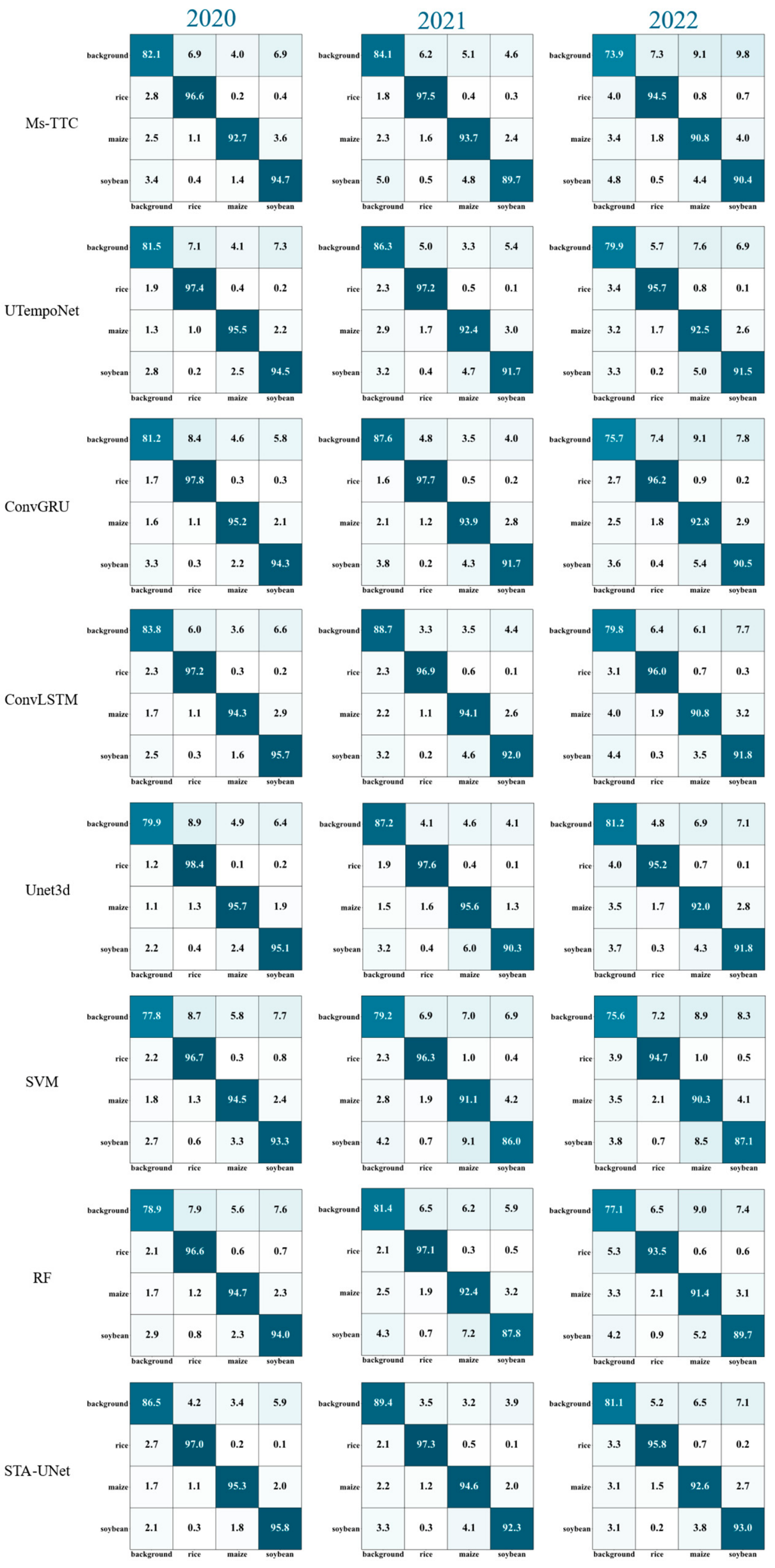
To further elucidate class-wise behavior, Figure 9 presents the confusion matrices for all models assessed on the 2020–2022 datasets. STA-UNet attains the highest accuracies across all years of analyses. Rice demonstrates superior separability, with per-class accuracies ranging from 95.8% to 97.3%; maize maintains accuracies between 92.6% and 95.3%; soybean reaches a range of 92.3% to 95.8%; and the background class is identified with accuracies from 81.1% to 89.4%. Overall, deep learning models outperform traditional machine learning methods. Both ConvLSTM and ConvGRU achieve performance levels comparable to those of STA-UNet yet remain slightly inferior in terms of OA. While Unet3d exhibits strong performance for rice (with accuracies ranging from 95.2% to 98.4%), it requires substantially more parameters and is less computationally efficient than its counterparts.

The specialized spatial-temporal networks Ms-TTC and UTempoNet yield mid-range results: Ms-TTC demonstrates relative stability for rice (with accuracies spanning from 94.5% to 97.5%) but shows pronounced fluctuations for soybean (from 89.7% to 94.7%), and UTempoNet experiences a significant decline in classification OA for soybean in the last two years, indicating potential sensitivity to inter-annual variations affecting this crop. Traditional SVM and RF display significant inter-annual volatility for soybean, with OA rates declining from over 93% in 2020 to ranges of 86.0–89.7% during the years 2021–2022. This trend indicates a reduced adaptability to inter-annual climatic variability. The analysis of confusion matrices further highlights class-specific peculiarities: rice exhibits the highest recognition ease due to its distinctive spectral characteristics; maize and soybean experience mutual misclassification at approximately 2.0%; conversely, background recognition proves most challenging across all models examined. While all methodologies experienced declines in performance in 2022, STA-UNet exhibits the least degradation. This robustness can be attributed to its spatial-temporal attention mechanism, which provides substantial evidence of its capability in learning deep spatial-temporal features effectively.

5.3. Analysis of Crop-Type Mapping

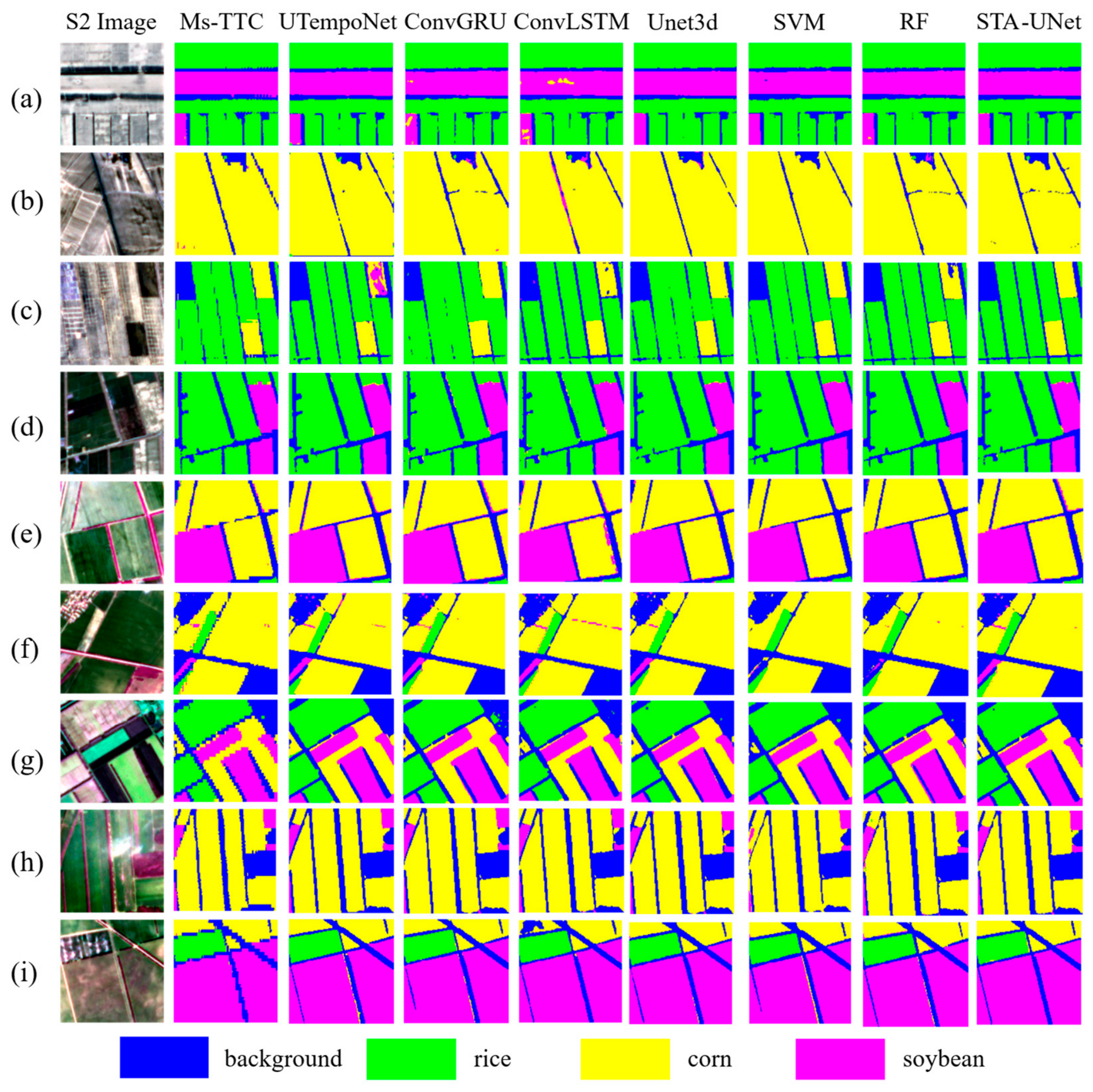
Figure 10 illustrates the classification results obtained from STA-UNet and seven comparative methods across nine representative parcels (Figure 10a–i) using imagery from multiple years. In Figure 10a, STA-UNet demonstrates superior performance, while Ms-TTC and UTempoNet show comparable results, albeit with slightly inferior boundary delineation. ConvGRU exhibits commendable boundary delineation yet experiences misclassification between maize and soybean; meanwhile, ConvLSTM encounters both diminished boundary delineation capabilities and more significant misclassifications compared to ConvGRU. In Figure 10b, the performance disparities become more pronounced. Several models—including Ms-TTC, UTempoNet, ConvLSTM, Unet3d, and SVM—exhibit notable deficiencies in boundary delineation as evidenced by the omission of critical boundary lines. Conversely, STA-UNet demonstrates only negligible confusion between background and maize classification. Figure 10c reveals that STA-UNet, Unet3d, and SVM present no apparent issues; however, Ms-TTC shows blurred boundaries, whilst UTempoNet suffers from substantial misclassification affecting large areas of maize-soybean differentiation. Additionally, ConvGRU is characterized by a marked decline in its boundary delineation efficacy. Figure 10d captures a relatively straightforward scene where most models perform on par with one another; only Unet3d displays minor issues related to boundary definition while ConvGRU incurs several misclassifications. In Figure 10e, ConvLSTM displays significant confusion between the corn and soybean classes, while traditional methods such as SVM and RF perform relatively better in this context. Furthermore, Ms-TTC displays inadequate boundary continuity. Figure 10f further substantiates the superiority of STA-UNet; although minor misclassifications are present, they remain negligible in impact. In contrast, other models exhibit varying levels of maize-soybean confusion; for instance, SVM and RF reveal severe discrepancies in certain areas characterized by background-soybean misclassification. Figure 10g depicts a complex scene that includes rice cultivation. In this scenario, UTempoNet performs comparably to STA-UNet, whereas Ms-TTC presents jagged boundaries and ConvGRU suffers from multi-class misclassification problems. The limitations of traditional methods become more pronounced in Figure 10h: both SVM and RF demonstrate marked misclassification issues, with RF even resulting in fragmented boundary lines. Additionally, Ms-TTC shows a lack of boundary sharpness. Finally, Figure 10i highlights various shortcomings across the different models examined herein. For instance, SVM incorrectly classifies some background boundaries as maize, UTempoNet encounters issues with broken boundaries and background-maize confusion, while Ms-TTC is notable for its jagged boundaries. Overall, with respect to boundary delineation, STA-UNet demonstrates superior performance across the majority of scenes. While Ms-TTC and UTempoNet approach the performance levels of STA-UNet in simpler scenarios, they exhibit shortcomings in complex environments. Regarding misclassification control, STA-UNet effectively confines errors within acceptable limits. In contrast, ConvGRU and ConvLSTM experience considerable misclassification in particular scenes, while SVM and RF are more susceptible to pronounced errors. In terms of scene adaptability, STA-UNet maintains consistent performance from simple to intricate farmland landscapes. This highlights the efficacy of its spatial-temporal attention mechanism in effectively capturing crop phenological dynamics and suppressing interference.

5.4. Ablation Experiment

To evaluate the effectiveness of key components and their contributions to overall network performance, a series of fine-grained ablation experiments is conducted. Building upon a base model, six configurations are systematically assessed: (1) Baseline: a simplified reference model that utilizes temporal average pooling instead of TAE, eliminates the CBA module, employs transposed-convolution upsampling in lieu of the DU module, and substitutes the AFF module with channel-wise concatenation followed by convolution; (2) Model-1 (CBA ablation): the CBA module is omitted from STA-UNet; (3) Model-2 (TAE ablation): the TAE module is replaced with temporal average pooling; (4) Model-3 (DU ablation): the DU module is substituted with transposed-convolution upsampling; (5) Model-4 (AFF ablation): the AFF module is exchanged for channel-wise concatenation followed by convolution; and (6) Full model: the complete STA-UNet.

Table 4. Ablation study results of the essential components of STA-UNet (%).

Year	Method	OA	mIoU	F1-Score	Precision	Recall
2020	Baseline	91.29	81.69	89.59	89.79	89.46
	Model-1	92.69	84.49	91.38	91.37	91.39
	Model-2	94.12	86.91	92.79	92.85	92.72
	Model-3	94.77	88.16	93.52	93.20	93.42
	Model-4	94.56	87.84	93.35	93.50	93.21
	STA-UNet	94.80	88.30	93.62	93.56	93.64
2021	Baseline	91.67	83.10	90.62	90.90	90.42
	Model-1	93.68	86.92	92.91	92.92	92.99
	Model-2	93.74	86.98	92.94	92.95	92.93
	Model-3	93.36	86.21	92.49	92.87	92.19
	Model-4	92.86	85.45	92.05	91.93	92.18
	STA-UNet	94.12	87.73	93.38	93.39	93.40
2022	Baseline	91.15	82.16	89.97	89.91	90.04
	Model-1	91.88	83.31	90.65	90.76	90.56
	Model-2	91.21	83.15	90.66	90.80	90.57
	Model-3	91.75	83.09	90.51	90.56	90.47
	Model-4	91.76	83.10	90.52	90.63	90.43
	STA-UNet	91.91	83.37	90.69	90.81	90.63

The optimal results are displayed in bold, while the second-optimal results are underlined.

reports the ablation results on the 2020, 2021, and 2022 datasets. The ablation results show that all four modules contribute to the final performance, but their relative importance varies across years. To avoid over-interpreting the comparison with the baseline, we further examine the performance drop from the full STA-UNet to each ablated model. In 2020, removing CBA caused the largest decrease in OA, mIoU, and F1-score, with drops of 2.11%, 3.81%, and 2.24%, respectively. From the perspective of network structure, this result suggests that CBA plays a key role at the entrance of the encoder by refining spatial–spectral responses before temporal aggregation. Once CBA is removed, noisy or weak parcel-related features are passed directly into the subsequent temporal encoder, which limits the quality of temporal feature modeling and leads to a larger performance drop. In contrast, the removal of TAE leads to moderate decreases in 2020. This suggests that TAE contributes mainly by reweighting and encoding discriminative temporal observations, but its effectiveness also depends on the quality of the spatial-spectral features provided by the encoder; therefore, when CBA is retained, part of the discriminative information can still be preserved.

The 2021 and 2022 results reveal different performance bottlenecks. In 2021, removing AFF produced the largest decline, with OA, mIoU, and F1-score decreasing by 1.26%, 2.28%, and 1.33%, respectively, followed by DU. From the architectural perspective, this indicates that when temporal cues are relatively stable, the main bottleneck shifts from temporal representation to feature reconstruction and cross-level information integration. AFF is located at the feature fusion stage and adaptively combines decoder features with attention-enhanced skip features; removing it weakens the interaction between low-level spatial details and high-level semantic-temporal features, which is particularly harmful for small and irregular parcels. The influence of DU and AFF further shows that the decoder is not only responsible for resolution recovery, but also for reorganizing spatial details after temporal encoding. DU improves boundary-adaptive upsampling, while AFF controls the fusion between decoder features and temporally enhanced skip features; therefore, removing either module can weaken the structural consistency of the final segmentation map. In 2022, removing TAE causes the largest OA decrease, while removing DU or AFF still produces consistent drops. This can be explained by the position of TAE in the network: it acts as the main temporal modeling unit before decoder reconstruction, so its removal directly weakens the network’s ability to distinguish reliable and unreliable phenological observations under stronger inter-annual variation and phenological inconsistency. Overall, these results show that the four modules contribute at different structural positions of STA-UNet.

5.5. Analysis of Generalization Ability

To comprehensively assess the practical applicability of the models, the ability to generalize is of paramount importance. Therefore, two complementary tests—spatial generalization and temporal generalization—are designed to evaluate STA-UNet and the comparison methods across different scenarios effectively.

The results for left-subregion spatial generalization (

Table 5. Comparison of various models in left-subregion spatial generalization tests in different years (%).

Year	Method	OA	mIoU	F1-Score	Precision	Recall
2020	Ms-TTC	82.42	69.05	81.21	81.02	81.54
	UTempoNet	76.07	59.07	72.41	78.04	73.08
	ConvGRU	81.11	66.79	79.49	79.79	79.80
	ConvLSTM	82.58	69.05	81.19	81.39	81.05
	Unet3d	77.67	62.65	76.34	78.68	75.54
	SVM	57.12	39.97	48.62	54.26	54.37
	RF	56.15	39.04	49.44	61.48	55.28
	STA-UNet	86.32	74.57	85.08	85.66	84.70
2021	Ms-TTC	82.86	69.45	81.51	83.27	82.35
	UTempoNet	85.76	74.08	84.89	84.88	85.28
	ConvGRU	76.74	61.96	75.89	80.85	77.07
	ConvLSTM	84.41	71.75	83.20	83.94	83.89
	Unet3d	83.52	69.65	81.41	83.85	81.96
	SVM	53.41	36.43	47.84	59.32	50.75
	RF	45.41	29.37	42.18	63.61	47.78
	STA-UNet	87.53	76.95	86.79	86.56	87.13
2022	Ms-TTC	83.79	69.97	81.97	83.34	81.40
	UTempoNet	80.52	64.54	77.59	82.25	77.56
	ConvGRU	72.85	54.48	69.85	75.43	70.57
	ConvLSTM	78.51	62.22	76.40	80.34	75.21
	Unet3d	79.74	63.72	77.19	80.58	76.87
	SVM	42.97	27.36	35.64	56.47	40.68
	RF	43.22	27.57	41.28	56.51	43.22
	STA-UNet	85.02	72.17	83.51	84.51	83.39

The optimal results are displayed in bold, while the second-optimal results are underlined.

) illuminate three key findings: (1) STA-UNet demonstrates superior spatial generalization performance across all years, achieving an average OA of 86.29% over three years, which reflects a 7.32% decline compared to the standard test average of 93.61%. This performance significantly exceeds that of other deep learning methods: Ms-TTC shows a drop of 8.65%, ConvLSTM has a reduction of 11.14%, UTempoNet exhibits an 11.88% decrease, Unet3d decreases by 12.86%, and ConvGRU presents a drop of 15.79%. (2) Traditional methods such as SVM and RF experience catastrophic declines in performance, with three-year average OAs diminishing by 39.25% and 42.71%, respectively—substantially inferior when compared to deep learning approaches. (3) Almost all models demonstrate enhanced spatial generalization in the year 2021 relative to the years 2020 and 2022, likely attributable to more uniform crop planting patterns within the study area during that year, subsequently minimizing the effects associated with shifts in spatial distribution.

The additional right-subregion spatial generalization results in

Table 6. Comparison of various models in the right-subregion spatial generalization test in different years (%).

Year	Method	OA	mIoU	F1-Score	Precision	Recall
2020	Ms-TTC	81.22	41.78	54.22	58.39	51.82
	UTempoNet	81.92	43.56	56.18	61.41	52.82
	ConvGRU	81.24	40.75	53.39	59.25	50.27
	ConvLSTM	80.60	41.35	54.12	58.81	51.32
	Unet3d	81.94	41.34	54.01	56.25	52.23
	SVM	73.98	58.70	41.41	47.91	40.85
	RF	75.09	60.12	41.34	44.78	40.95
	STA-UNet	82.25	44.18	56.85	63.18	53.47
2021	Ms-TTC	82.85	62.74	75.45	77.25	73.85
	UTempoNet	83.01	61.65	74.47	76.82	73.38
	ConvGRU	81.25	60.65	73.87	74.87	73.06
	ConvLSTM	82.05	61.32	74.36	74.77	73.97
	Unet3d	82.62	61.02	74.89	76.33	73.60
	SVM	77.55	59.84	62.84	66.16	62.98
	RF	68.65	52.26	57.05	64.58	55.92
	STA-UNet	82.93	61.67	74.62	75.01	74.32
2022	Ms-TTC	77.15	54.76	68.95	68.73	69.86
	UTempoNet	73.17	52.93	67.26	67.42	68.73
	ConvGRU	77.89	52.49	66.78	66.20	67.94
	ConvLSTM	78.80	54.26	68.31	70.17	66.73
	Unet3d	74.58	49.48	64.47	61.33	69.10
	SVM	60.25	43.11	38.76	44.76	45.96
	RF	52.75	35.82	39.18	42.06	44.51
	STA-UNet	78.84	55.23	69.31	69.67	69.14

The optimal results are displayed in bold, while the second-optimal results are underlined.

indicate that STA-UNet achieves the highest three-year average OA, mIoU, and F1-score, while exhibiting a performance profile that differs substantially from that observed in the left-subregion benchmark. Compared with Table 5, the reduction in OA is relatively moderate, whereas the declines in mIoU and F1-score are considerably larger. This pattern can be attributed to the class composition reported in Table 1, where rice accounts for 68.75–79.22% of labeled pixels in the right subregion, while maize and soybean remain minority classes, with maize representing only 1.53% in 2020. Consequently, OA is primarily driven by correctly classified rice pixels and remains close to 80% for most deep learning models, whereas mIoU and F1-score more sensitively reflect the degradation in class-wise overlap and balanced recognition. The 2020 results illustrate this effect most clearly: although deep learning models obtain comparable OA values, their mIoU and F1-score are restricted to 40.75–44.18% and 53.39–56.85%, respectively. These findings demonstrate that the right-subregion experiment complements the left-subregion evaluation by revealing model behavior under severe class imbalance, where class-wise metrics are necessary for interpreting spatial generalization beyond OA. Under this challenging setting, the relative advantage of STA-UNet suggests that its spatial-temporal attention and feature fusion design helps retain more transferable crop representations. By emphasizing discriminative phenological stages and boundary-sensitive spatial features, STA-UNet better alleviates the performance degradation associated with minority-class underrepresentation and regional distribution shift.

The temporal generalization tests (

Table 7. Performance evaluation of various models in temporal generalization tests (%).

Training Year	Testing Year	Method	OA	mIoU	F1-Score	Precision	Recall
2020	2021	Ms-TTC	84.79	72.60	83.73	84.36	84.62
		UTempoNet	78.31	63.67	77.02	77.67	77.02
		ConvGRU	87.24	75.95	86.02	86.33	85.77
		ConvLSTM	82.73	69.90	81.89	82.29	83.14
		Unet3d	84.64	71.87	83.08	83.44	83.39
		SVM	67.13	50.52	61.03	68.09	64.86
		RF	46.09	29.95	43.91	71.62	48.86
		STA-UNet	90.16	80.84	89.24	89.27	89.47
	2022	Ms-TTC	77.02	62.23	76.22	77.00	77.57
		UTempoNet	78.31	63.67	77.02	77.67	77.02
		ConvGRU	76.99	61.75	75.73	76.36	75.42
		ConvLSTM	77.32	62.65	76.56	77.32	78.10
		Unet3d	78.70	64.10	77.72	78.23	78.95
		SVM	55.70	38.60	55.95	63.30	58.42
		RF	71.87	56.10	71.00	72.61	72.28
		STA-UNet	80.19	66.36	79.14	80.26	79.20
2021	2020	Ms-TTC	74.82	59.06	73.00	73.98	75.21
		UTempoNet	81.84	67.94	80.40	80.12	80.94
		ConvGRU	75.92	60.59	74.69	76.79	76.98
		ConvLSTM	72.45	56.94	71.74	75.58	75.59
		Unet3d	82.51	68.70	80.83	80.72	82.38
		SVM	34.86	21.11	34.41	52.49	39.73
		RF	67.01	50.38	65.34	66.38	66.69
		STA-UNet	84.76	65.32	77.55	82.00	77.32
	2022	Ms-TTC	71.44	56.27	71.23	77.09	73.47
		UTempoNet	70.46	54.48	68.99	75.59	72.30
		ConvGRU	66.65	49.04	65.20	71.80	68.52
		ConvLSTM	74.49	59.40	73.90	77.97	75.91
		Unet3d	75.23	59.54	74.33	78.05	75.85
		SVM	21.82	12.24	16.43	61.01	29.87
		RF	53.62	36.63	53.13	62.50	56.11
		STA-UNet	76.10	61.11	75.67	77.26	77.74
2022	2020	Ms-TTC	83.16	69.38	81.31	81.06	82.01
		UTempoNet	78.04	61.83	74.73	74.98	76.52
		ConvGRU	76.26	59.28	72.61	73.24	74.43
		ConvLSTM	68.52	51.91	67.07	70.06	68.95
		Unet3d	77.90	61.52	74.93	74.95	75.61
		SVM	62.25	45.19	55.31	63.26	58.54
		RF	64.09	47.16	60.08	66.91	63.70
		STA-UNet	84.53	71.51	82.90	82.67	83.33
	2021	Ms-TTC	87.04	75.14	85.54	87.60	84.56
		UTempoNet	88.50	77.75	87.29	88.57	86.60
		ConvGRU	86.07	73.50	84.49	87.30	83.31
		ConvLSTM	86.28	73.83	84.62	86.63	83.71
		Unet3d	87.70	75.90	85.98	88.25	84.93
		SVM	48.82	32.30	45.66	57.31	48.10
		RF	40.34	25.26	36.98	67.23	44.00
		STA-UNet	88.86	78.68	87.95	88.74	87.58

The optimal results are displayed in bold, while the second-optimal results are underlined.

) demonstrate that STA-UNet consistently achieves the best or near-best performance across cross-year scenarios, with distinct inter-annual differences observed. When trained on the 2020 dataset and tested on the 2021 dataset, STA-UNet attains an OA of 90.16%, significantly surpassing other deep learning approaches such as Ms-TTC (84.79%) and ConvGRU (87.24%), as well as traditional methods like SVM (67.13%) and RF (46.09%). Furthermore, when trained on data from 2020 and evaluated using the 2022 dataset, STA-UNet maintains a commendable OA of 80.19%, indicating strong long-term temporal generalization capabilities.

However, the cross-year results also indicate that temporal transfer remains sensitive to stronger inter-annual shifts. The most evident degradation occurs when the model is trained on 2021 and tested on 2022, where STA-UNet obtains an OA of 76.10%. Compared with its standard 2021 test OA of 94.12%, this corresponds to an 18.02 percentage-point decrease. A more direct explanation is the reduced temporal coverage and lower target-year separability of the 2022 data. Specifically, the maximum temporal length decreases from 99 observations in 2021 to 95 in 2022, and the full phenological-window coverage of the middle-subregion set decreases from 100% in 2021 to 98.1% in 2022. The 2022 target year is also consistently more difficult in the reported results: in the standard test, STA-UNet’s OA decreases from 94.12% in 2021 to 91.91% in 2022, and all compared baselines show OA drops of 1.15–3.05 percentage points; in the left-subregion test, STA-UNet also decreases from 87.53% to 85.02%. Therefore, the 2021-to-2022 transfer degradation is better interpreted as a source-target mismatch between the more complete 2021 temporal observations and the reduced temporal coverage and lower separability of the 2022 target data.

Synthesizing the spatial and temporal findings, STA-UNet demonstrates strong environmental adaptability under both balanced and imbalanced transfer settings. In the left-subregion test, STA-UNet maintains high cross-region OA with an average OA of 86.29%. In the right-subregion stress test, the average OA remains competitive at 81.34%, but the much lower mIoU and F1-score values show that rice-dominated class imbalance makes minority-class recognition the main limitation. Together with the temporal generalization results, these experiments provide reliable technical support for sustained large-scale crop mapping in the Sanjiang Plain while also clarifying the remaining difficulty of mapping minority crops in rice-dominated regions.

6. Discussion

The main implication of these results is that crop mapping from irregular Sentinel-2 time series should be evaluated not only by overall accuracy, but also by how well a model handles temporal gaps, parcel boundaries, and regional distribution shifts. The consistent gains of STA-UNet in the standard tests suggest that jointly modeling spatial-spectral responses and temporal attention is useful when cloud cover and phenological variation make individual observations unreliable. However, the generalization results also reveal an important caveat: in the rice-dominated right subregion, OA remains relatively high while mIoU and F1-score decrease markedly, showing that class imbalance can hide weak recognition of minority crops if only aggregate OA is considered. Similarly, the cross-year tests indicate that inter-annual changes in crop distribution and phenology still produce notable domain shifts. Therefore, although the proposed architecture improves robustness under complex remote sensing conditions, its practical deployment should rely on class-wise metrics and additional validation in imbalanced or phenologically shifted regions; future work should further strengthen minority-crop recognition, boundary-specific evaluation, and multisource feature integration.

7. Conclusions

This study proposes STA-UNet, a phenology-guided and boundary-aware spatial-temporal U-Net for crop mapping from irregular Sentinel-2 time series in the Sanjiang Plain. The model is designed to mitigate accuracy degradation caused by cloud-induced temporal discontinuities, regional phenological variation, and the loss of fine parcel boundaries during spatial reconstruction. Its core technical advantages can be summarized as follows: the CBA module enhances crop-related spectral-spatial responses; the TAE module adaptively captures key phenological information while reducing the influence of missing or cloud-contaminated observations; the DU and AFF modules improve boundary-aware upsampling and adaptive feature fusion. Experimental results from multi-year classification, ablation studies, spatial generalization tests on both left and right subregions, and temporal generalization tests demonstrate that STA-UNet consistently achieves competitive performance compared with existing deep learning and traditional methods. These results indicate that STA-UNet provides an effective and transferable framework for large-scale crop mapping in cloud-prone and phenologically complex agricultural regions. Future work will focus on improving minority-crop recognition under imbalanced regional distributions and extending the model to broader agricultural areas and multisource time-series observations.

References

1. Weiss, M.; Jacob, F.; Duveiller, G. Remote sensing for agricultural applications: A meta-review. Remote Sens. Environ. 2020, 236, 111402. [Google Scholar] [CrossRef]
2. Liu, L.; Xiao, X.; Qin, Y.; Wang, J.; Xu, X.; Hu, Y.; Qiao, Z. Mapping cropping intensity in China using time series Landsat and Sentinel-2 images and Google Earth Engine. Remote Sens. Environ. 2020, 239, 111624. [Google Scholar] [CrossRef]
3. Gallego, F.J.; Kussul, N.; Skakun, S.; Kravchenko, O.; Shelestov, A.; Kussul, O. Efficiency assessment of using satellite data for crop area estimation in Ukraine. Int. J. Appl. Earth Obs. Geoinf. 2014, 29, 22–30. [Google Scholar] [CrossRef]
4. Carfagna, E.; Gallego, F.J. Using remote sensing for agricultural statistics. Int. Stat. Rev. 2006, 73, 389–404. [Google Scholar] [CrossRef]
5. Fan, L.; Xia, L.; Yang, J.; Sun, X.; Wu, S.; Qiu, B.; Chen, J.; Wu, W.; Yang, P. A temporal-spatial deep learning network for winter wheat mapping using time-series Sentinel-2 imagery. ISPRS-J. Photogramm. Remote Sens. 2024, 214, 48–64. [Google Scholar] [CrossRef]
6. Vuolo, F.; Neuwirth, M.; Immitzer, M.; Atzberger, C.; Ng, W.T. How much does multi-temporal Sentinel-2 data improve crop type classification? Int. J. Appl. Earth Obs. Geoinf. 2018, 72, 122–130. [Google Scholar] [CrossRef]
7. Belgiu, M.; Csillik, O. Sentinel-2 cropland mapping using pixel-based and object-based time-weighted dynamic time warping analysis. Remote Sens. Environ. 2018, 204, 509–523. [Google Scholar] [CrossRef]
8. Zhong, L.; Hu, L.; Zhou, H. Deep learning based multi-temporal crop classification. Remote Sens. Environ. 2019, 221, 430–443. [Google Scholar] [CrossRef]
9. Kussul, N.; Lavreniuk, M.; Skakun, S.; Shelestov, A. Deep Learning Classification of Land Cover and Crop Types Using Remote Sensing Data. IEEE Geosci. Remote Sens. Lett. 2017, 14, 778–782. [Google Scholar] [CrossRef]
10. Wardlow, B.D.; Egbert, S.L. Large-area crop mapping using time-series MODIS 250 m NDVI data: An assessment for the U.S. Central Great Plains. Remote Sens. Environ. 2008, 112, 1096–1116. [Google Scholar] [CrossRef]
11. Gella, G.W.; Bijker, W.; Belgiu, M. Mapping crop types in complex farming areas using SAR imagery with dynamic time warping. ISPRS-J. Photogramm. Remote Sens. 2021, 175, 171–183. [Google Scholar] [CrossRef]
12. Maulik, U.; Chakraborty, D. Learning with transductive SVM for semisupervised pixel classification of remote sensing imagery. ISPRS-J. Photogramm. Remote Sens. 2013, 77, 66–78. [Google Scholar] [CrossRef]
13. Rodriguez-Galiano, V.F.; Ghimire, B.; Rogan, J.; Chica-Olmo, M.; Rigol-Sanchez, J.P. An assessment of the effectiveness of a random forest classifier for land-cover classification. ISPRS-J. Photogramm. Remote Sens. 2012, 67, 93–104. [Google Scholar] [CrossRef]
14. Rußwurm, M.; Körner, M. Self-attention for raw optical Satellite Time Series Classification. ISPRS-J. Photogramm. Remote Sens. 2020, 169, 421–435. [Google Scholar] [CrossRef]
15. Mobarakeh, Z.M.; Pourmanafi, S.; Ahmadi, M. Employing sentinel-2 time-series and noisy data quality control enhance crop classification in arid environments: A comparison of machine learning and deep learning methods. Int. J. Appl. Earth Obs. Geoinf. 2025, 142, 104678. [Google Scholar] [CrossRef]
16. Meng, S.; Wang, X.; Hu, X.; Luo, C.; Zhong, Y. Deep learning-based crop mapping in the cloudy season using one-shot hyperspectral satellite imagery. Comput. Electron. Agric. 2021, 186, 106188. [Google Scholar] [CrossRef]
17. Adrian, J.; Sagan, V.; Maimaitijiang, M. Sentinel SAR-optical fusion for crop type mapping using deep learning and Google Earth Engine. ISPRS-J. Photogramm. Remote Sens. 2021, 175, 215–235. [Google Scholar] [CrossRef]
18. Su, T.; Zhang, S. Object-based crop classification in Hetao irrigation zone by using deep learning and region merging optimization. Comput. Electron. Agric. 2023, 214, 108284. [Google Scholar] [CrossRef]
19. Wang, Y.; Feng, L.; Zhang, Z.; Tian, F. An unsupervised domain adaptation deep learning method for spatial and temporal transferable crop type mapping using Sentinel-2 imagery. ISPRS-J. Photogramm. Remote Sens. 2023, 199, 102–117. [Google Scholar] [CrossRef]
20. Xia, L.; Zhao, F.; Chen, J.; Yu, L.; Lu, M.; Yu, Q.; Liang, S.; Fan, L.; Sun, X.; Wu, S.; et al. A full resolution deep learning network for paddy rice mapping using Landsat data. ISPRS-J. Photogramm. Remote Sens. 2022, 194, 91–107. [Google Scholar] [CrossRef]
21. Cai, Z.; Wei, H.; Hu, Q.; Zhou, W.; Zhang, X.; Jin, W.; Wang, L.; Yu, S.; Wang, Z.; Xu, B.; et al. Learning spectral-spatial representations from VHR images for fine-scale crop type mapping: A case study of rice-crayfish field extraction in South China. ISPRS-J. Photogramm. Remote Sens. 2023, 199, 28–39. [Google Scholar] [CrossRef]
22. Mohammadi, S.; Belgiu, M.; Stein, A. Improvement in crop mapping from satellite image time series by effectively supervising deep neural networks. ISPRS-J. Photogramm. Remote Sens. 2023, 198, 272–283. [Google Scholar] [CrossRef]
23. Pelletier, C.; Webb, G.I.; Petitjean, F. Temporal convolutional neural network for the classification of satellite image time series. Remote Sens. 2019, 11, 523. [Google Scholar] [CrossRef]
24. Zhang, C.; Sargent, I.; Pan, X.; Li, H.; Gardiner, A.; Hare, J.; Atkinson, P.M. A hybrid MLP-CNN classifier for very fine resolution remotely sensed image classification. ISPRS-J. Photogramm. Remote Sens. 2018, 140, 133–144. [Google Scholar] [CrossRef]
25. Gao, M.; Lu, T.; Wang, L. Crop mapping based on Sentinel-2 images using semantic segmentation model of attention mechanism. Sensors 2023, 23, 7008. [Google Scholar] [CrossRef]
26. Interdonato, R.; Ienco, D.; Gaetano, R.; Ose, K. DuPLO: A DUal view Point deep Learning architecture for time series classification. ISPRS-J. Photogramm. Remote Sens. 2019, 149, 91–104. [Google Scholar] [CrossRef]
27. Huang, X.; Wang, H.; Li, X. A multi-scale semantic feature fusion method for remote sensing crop classification. Comput. Electron. Agric. 2024, 224, 109185. [Google Scholar] [CrossRef]
28. Yang, H.; Yu, H.; Zheng, K.; Hu, J.; Tao, T.; Zhang, Q. Hyperspectral image classification based on interactive Transformer and CNN with multilevel feature fusion network. IEEE Geosci. Remote Sens. Lett. 2023, 20, 1–5. [Google Scholar] [CrossRef]
29. Gui, B.; Sam, L.; Bhardwaj, A.; Gómez, D.S.; Peñaloza, F.G.; Buchroithner, M.F.; Green, D.R. SAGRNet: A novel object-based graph convolutional neural network for diverse vegetation cover classification in remotely-sensed imagery. ISPRS-J. Photogramm. Remote Sens. 2025, 227, 99–124. [Google Scholar] [CrossRef]
30. Yang, T.; Xiao, S.; Qu, J. D3GNN: Double dual dynamic graph neural network for multisource remote sensing data classification. Int. J. Appl. Earth Obs. Geoinf. 2025, 139, 104496. [Google Scholar] [CrossRef]
31. Hong, D.; Gao, L.; Yao, J.; Zhang, B.; Plaza, A.; Chanussot, J. Graph convolutional networks for hyperspectral image classification. IEEE Trans. Geosci. Remote Sens. 2021, 59, 5966–5978. [Google Scholar] [CrossRef]
32. Zhang, C.; Wang, J.; Yao, K. Global random graph convolution network for hyperspectral image classification. Remote Sens. 2021, 13, 2285. [Google Scholar] [CrossRef]
33. Wan, S.; Pan, S.; Zhong, P.; Chang, X.; Yang, J.; Gong, C. Dual interactive graph convolutional networks for hyperspectral image classification. IEEE Trans. Geosci. Remote Sens. 2021, 60, 5510214. [Google Scholar] [CrossRef]
34. Wu, G.; Al-qaness, M.A.; Al-Alimi, D.; Dahou, A.; Abd Elaziz, M.; Ewees, A.A. Hyperspectral image classification using graph convolutional network: A comprehensive review. Expert Syst. Appl. 2024, 257, 125106. [Google Scholar] [CrossRef]
35. Bağcı, R.Ş.; Acar, E.; Türk, Ö. Identification of cotton and corn plant areas by employing deep transformer encoder approach and different time series satellite images: A case study in Diyarbakir, Turkey. Comput. Electron. Agric. 2023, 209, 107838. [Google Scholar] [CrossRef]
36. Chen, C.; Zhang, C.; Zhao, L.; Yang, C.; Yao, X.; Fu, B. Soybean cultivation and crop rotation monitoring based on multi-source remote sensing data and Bi-LSTM enhanced model. Comput. Electron. Agric. 2025, 239, 110959. [Google Scholar] [CrossRef]
37. Feng, F.; Gao, M.; Liu, R.; Yao, S.; Yang, G. A deep learning framework for crop mapping with reconstructed Sentinel-2 time series images. Comput. Electron. Agric. 2023, 213, 108227. [Google Scholar] [CrossRef]
38. Wang, Y.; Feng, L.; Sun, W.; Wang, L.; Yang, G.; Chen, B. A lightweight CNN-Transformer network for pixel-based crop mapping using time-series Sentinel-2 imagery. Comput. Electron. Agric. 2024, 226, 109370. [Google Scholar] [CrossRef]
39. Guo, X.; Feng, Q.; Guo, F. CMTNet: A hybrid CNN-transformer network for UAV-based hyperspectral crop classification in precision agriculture. Sci. Rep. 2025, 15, 12383. [Google Scholar] [CrossRef] [PubMed]
40. Xu, Z.; Zhang, W.; Zhang, T.; Yang, Z.; Li, J. Efficient Transformer for remote sensing image segmentation. Remote Sens. 2021, 13, 3585. [Google Scholar] [CrossRef]
41. Zhang, X.; Wei, H.; Shao, Y.; Luan, H.; Wang, D.H. Transformer-based dual-branch spatial–temporal–spectral feature fusion network for paddy rice mapping. Remote Sens. 2025, 17, 1999. [Google Scholar] [CrossRef]
42. Cai, Z.; Hu, Q.; Zhang, X.; Yang, J.; Wei, H.; Wang, J.; Zeng, Y.; Yin, G.; Li, W.; You, L.; et al. Improving agricultural field parcel delineation with a dual branch spatiotemporal fusion network by integrating multimodal satellite data. ISPRS-J. Photogramm. Remote Sens. 2023, 205, 34–49. [Google Scholar] [CrossRef]
43. Deressu, T.F.; Bojer, A.K.; Debelee, T.G.; Negera, W.G.; Nadarajah, S.; Gebissa, K.W. Enhancing land use and land cover classification with deep learning-based satellite imagery segmentation. Int. J. Appl. Earth Obs. Geoinf. 2025, 144, 104839. [Google Scholar] [CrossRef]
44. Ge, J.; Zhang, H.; Zuo, L.; Xu, L.; Jiang, J.; Song, M.; Ding, Y.; Xie, Y.; Wu, F.; Wang, C.; et al. Large-scale rice mapping under spatiotemporal heterogeneity using multi-temporal SAR images and explainable deep learning. ISPRS-J. Photogramm. Remote Sens. 2025, 220, 395–412. [Google Scholar] [CrossRef]
45. Ashraf, M.; Chen, L.; Innab, N.; Umer, M.; Baili, J.; Kim, T.H.; Ashraf, I. Novel 3-D deep neural network architecture for crop classification using remote sensing-based hyperspectral images. IEEE J. Sel. Top. Appl. Earth Obs. Remote Sens. 2024, 17, 12649–12665. [Google Scholar] [CrossRef]
46. Ji, S.; Zhang, C.; Xu, A.; Shi, Y.; Duan, Y. 3D convolutional neural networks for crop classification with multi-temporal remote sensing images. Remote Sens. 2018, 10, 75. [Google Scholar] [CrossRef]
47. Wittstruck, L.; Jarmer, T.; Waske, B. Multi-stage feature fusion of multispectral and SAR satellite images for seasonal crop-type mapping using an adapted 3D U-Net. Remote Sens. 2024, 16, 3115. [Google Scholar] [CrossRef]
48. Ballas, N.; Yao, L.; Pal, C.; Courville, A. Delving deeper into convolutional networks for learning video representations. arXiv 2015, arXiv:1511.06432. [Google Scholar] [CrossRef]
49. Cai, Z.; Xu, B.; Yu, Q.; Zhang, X.; Yang, J.; Wei, H.; Li, S.; Song, Q.; Xiong, H.; Wu, H.; et al. A cost-effective and robust mapping method for diverse crop types using weakly supervised semantic segmentation with sparse point samples. ISPRS-J. Photogramm. Remote Sens. 2024, 218, 260–276. [Google Scholar] [CrossRef]
50. Rußwurm, M.; Körner, M. Convolutional LSTMs for cloud-robust segmentation of remote sensing imagery. arXiv 2018, arXiv:1811.02471. [Google Scholar] [CrossRef]
51. Blaga, B.-C.-Z.; Nedevschi, S. Semantic segmentation of remote sensing images with Transformer-based U-Net and guided focal-axial attention. IEEE J. Sel. Top. Appl. Earth Obs. Remote Sens. 2024, 17, 18303–18318. [Google Scholar] [CrossRef]
52. Bian, Y.; Li, L.; Jing, W. CACPU-Net: Channel attention U-net constrained by point features for crop type mapping. Front. Plant Sci. 2022, 13, 1030595. [Google Scholar] [CrossRef] [PubMed]
53. Zhao, J.; Wang, J.; Qian, H.; Zhan, Y.; Lei, Y. Extraction of winter-wheat planting areas using a combination of U-Net and CBAM. Agronomy 2022, 12, 2965. [Google Scholar] [CrossRef]
54. Hao, P.; Di, L.; Zhang, C.; Guo, L. Transfer Learning for Crop classification with Cropland Data Layer data (CDL) as training samples. Sci. Total Environ. 2020, 733, 138869. [Google Scholar] [CrossRef]
55. Hu, Y.; Zeng, H.; Tian, F.; Zhang, M.; Wu, B.; Gilliams, S.; Li, S.; Li, Y.; Lu, Y.; Yang, H. An interannual transfer learning approach for crop classification in the Hetao Irrigation District, China. Remote Sens. 2022, 14, 1208. [Google Scholar] [CrossRef]
56. Nyborg, J.; Pelletier, C.; Lefevre, S.; Assent, I. TimeMatch: Unsupervised cross-region adaptation by temporal shift estimation. ISPRS-J. Photogramm. Remote Sens. 2022, 188, 301–313. [Google Scholar] [CrossRef]
57. Antonijevic, O.; Jelic, S.; Bajat, B.; Kilibarda, M. Transfer learning approach based on satellite image time series for the crop classification problem. J. Big Data. 2023, 10, 54. [Google Scholar] [CrossRef]
58. Pham, V.-D.; Tetteh, G.; Thiel, F.; Erasmi, S.; Schwieder, M.; Frantz, D.J.; van der Linden, S. Temporally transferable crop mapping with temporal encoding and deep learning augmentations. Int. J. Appl. Earth Obs. Geoinf. 2024, 129, 103867. [Google Scholar] [CrossRef]
59. Peng, S.; Zhang, L.; Xie, R.; Qu, Y. CSTN: A cross-region crop mapping method integrating self-training and contrastive domain adaptation. Int. J. Appl. Earth Obs. Geoinf. 2025, 136, 104379. [Google Scholar] [CrossRef]
60. Drusch, M.; Del Bello, U.; Carlier, S.; Colin, O.; Fernandez, V.; Gascon, F.; Hoersch, B.; Isola, C.; Laberinti, P.; Martinort, P.; et al. Sentinel-2: ESA’s optical high-resolution mission for GMES operational services. Remote Sens. Environ. 2012, 120, 25–36. [Google Scholar] [CrossRef]
61. Tang, P.; Chanussot, J.; Guo, S.; Zhang, W.; Qie, L.; Zhang, P.; Fang, H.; Du, P. Deep learning with multi-scale temporal hybrid structure for robust crop mapping. ISPRS-J. Photogramm. Remote Sens. 2024, 209, 117–132. [Google Scholar] [CrossRef]
62. Rustowicz, R.M.; Cheong, R.; Wang, L.; Ermon, S.; Burke, M.; Lobell, D. Semantic Segmentation of Crop Type in Africa: A novel dataset and analysis of deep learning methods. In Proceedings of the IEEE/CVF Conference on Computer Vision and Pattern Recognition (CVPR); IEEE: New York, NY, USA, 2019; pp. 75–82. [Google Scholar] [CrossRef]
63. Mammone, A.; Turchi, M.; Cristianini, N. Support vector machines. Wiley Interdiscip. Rev. Comput. Stat. 2009, 1, 283–289. [Google Scholar] [CrossRef]
64. Pal, M. Random forest classifier for remote sensing classification. Int. J. Remote Sens. 2005, 26, 217–222. [Google Scholar] [CrossRef]
Figure 1. Crop distribution map and administrative divisions of the Sanjiang Plain in 2020. Crop distribution data are derived from the remote sensing monitoring dataset of primary crop planting distributions in the Sanjiang Plain from 2020 to 2022, publicly available through SciDB (https://www.scidb.cn (accessed on 14 March 2025)). The inset in the lower right shows the location of the Sanjiang Plain in China.
Remotesensing 18 01677 g001
Figure 2. Distribution of sample parcels in the study area (2020). The underlying crop distribution data are derived from the remote sensing monitoring dataset of primary crop planting distributions in the Sanjiang Plain from 2020 to 2022, publicly available through SciDB (https://www.scidb.cn); sample parcels were generated through parcel extraction, quality screening, and stratified sampling based on this dataset.
Remotesensing 18 01677 g002
Figure 3. Workflow of the proposed crop classification framework.
Remotesensing 18 01677 g003
Figure 4. Network architecture of the STA-UNet.
Remotesensing 18 01677 g004
Figure 5. The architecture of CBA module.
Remotesensing 18 01677 g005
Figure 6. The architecture of TAE module.
Remotesensing 18 01677 g006
Figure 7. The architecture of DU module.
Remotesensing 18 01677 g007
Figure 8. The architecture of AFF module.
Remotesensing 18 01677 g008
Figure 9. Confusion matrices of different models across years. Rows denote ground-truth classes and columns denote predicted classes. Values are row-normalized percentages.
Remotesensing 18 01677 g009
Figure 10. Mapping results of different methods in different years and regions. Panels (ac) show 2020 examples, panels (df) show 2021 examples, and panels (gi) show 2022 examples.
Remotesensing 18 01677 g010