Surface-Subsurface Thermal Correspondence over Coal Fire Areas with UAV Thermal Infrared Remote Sensing and Subsurface Temperature Field Reconstruction

Highlights

What are the main findings?

• A spatial-structure-constrained MGSM–RBF method was developed that reconstructs the three-dimensional subsurface temperature field and identifies three fire-source centers, with primary combustion concentrated at depths of 30–55 m.
• A quantitative framework was developed to characterize the spatial offset between surface thermal anomaly centers and subsurface fire sources, revealing a non-vertical, coal-seam-controlled relationship with offset coefficients of 0.19–0.31.

What are the implications of the main findings?

• The results improve the reliability of interpreting UAV-derived thermal anomalies for subsurface fire source localization.
• The site-specific offset scale provides a preliminary reference for candidate drilling zones under similar steeply dipping, borehole-constrained conditions.

Abstract

Underground coal fires are persistent subsurface hazards threatening energy resources. UAV thermal infrared remote sensing provides high-resolution observations of surface thermal anomalies, but these signals may be spatially offset from underlying fire sources. An integrated framework was developed for subsurface temperature-field reconstruction and surface–subsurface correspondence and offset analysis. Surface thermal anomaly centers were extracted using statistical thresholding, adaptive kernel density estimation, and intensity-weighted centroids. Subsurface temperature fields were reconstructed using an MGSM-RBF model that combines multi-Gaussian fire-source representation with residual correction. The framework was applied to the Sandaoba coal fire area using UAV thermal infrared data and 370 borehole temperature measurements from 39 boreholes, covering depths of approximately 0–85 m. Reconstruction accuracy was evaluated using spatially buffered cross-validation and compared with eight baseline methods. MGSM–RBF achieved the best performance, with RMSE = 92.49 $°\mathrm{C}$, MAE = 61.26 $°\mathrm{C}$, and $R^2$ = 0.81. Two surface thermal anomaly centers and three subsurface fire sources were identified, with primary combustion concentrated at 30–55 m depths. Surface anomalies were not vertical projections of subsurface sources. The horizontal offsets were approximately one-fifth to one-third of burial depth, reflecting depth-dependent and multi-source-controlled surface thermal responses. These findings support UAV-based coal fire interpretation and fire-control planning.

1. Introduction

Underground coal fires are persistent subsurface combustion hazards characterized by strong concealment, long burning duration, and complex spatial distribution, posing serious threats to the utilization of coal resources and ecological security [1,2,3]. They are widespread in major coal-producing countries such as China, India, and the United States [4]. In addition to causing substantial losses of valuable coal resources, coal fires release large amounts of greenhouse gases, including $C{O}_2$ and $C{H}_4$, as well as harmful pollutants such as carbon monoxide and sulfur oxides, thereby severely degrading air quality and intensifying climate change. Meanwhile, prolonged combustion could also trigger a series of geological and environmental problems, such as surface cracking, ground subsidence, and severe degradation of soil and water resources, ultimately threatening regional ecological security and sustainable development [5,6]. Therefore, monitoring and remediation of coal fire areas are of great importance.

Accurate detection of coal fires and precise localization of subsurface fire sources are essential for effective prevention and suppression in coal fire areas. Traditional approaches, such as geophysical and geochemical methods, generally provide high detection accuracy for coal fires. However, they are often constrained by limited spatial coverage, high operational costs, and significant safety risks, making them inadequate for rapid monitoring in complex fire environments [7]. Remote sensing technologies, characterized by large-area coverage, non-contact observation, and high efficiency, offer an effective alternative for coal fire monitoring. By capturing indirect surface responses, such as thermal anomalies, ground deformation and gas emissions, coal fires could be efficiently detected and spatially characterized [8,9,10]. Among these approaches, satellite-based remote sensing is suitable for regional-scale monitoring, but its relatively coarse spatial resolution limits its ability to detect small-scale or concealed coal fires. In contrast, unmanned aerial vehicle (UAV)-based thermal infrared remote sensing offers higher spatial resolution and greater operational flexibility, making it particularly advantageous for the fine-scale characterization of surface thermal anomalies [11].

In recent years, the application of UAV-based remote sensing for coal fire detection has advanced considerably, with notable progress in thermal anomaly identification and three-dimensional representation [12,13]. However, UAV-based thermal infrared observations primarily capture surface temperature distributions, which reflect the indirect response of subsurface combustion through heat conduction and convection rather than the fire sources themselves. Consequently, surface thermal anomalies are commonly used to infer the spatial distribution of subsurface fire sources in practical applications.

Nevertheless, the relationship between surface thermal anomalies and subsurface fire sources is inherently complex. Heat transfer processes are strongly influenced by factors such as anisotropic thermal conductivity, coal seam inclination, overburden structure, and fracture development, often resulting in significant spatial offsets between surface thermal signals and the actual fire source locations. Ignoring this offset and relying solely on surface thermal anomalies for borehole placement may lead to substantial engineering errors. However, there are relatively few studies on the spatial correspondence between surface observations and subsurface fire sources.

This limitation is largely due to the difficulty in obtaining high-resolution three-dimensional subsurface temperature fields. Existing reconstruction methods mainly include numerical simulation [14] and geostatistical interpolation [15]. Numerical simulations often rely on simplified assumptions (e.g., homogeneous media and idealized boundary conditions), limiting their ability to represent complex heat transfer processes. Geostatistical interpolation based on borehole temperature data can be used to reconstruct subsurface temperature fields. However, it typically assumes a stationary random field and is not well suited to the highly heterogeneous sampling pattern of coal fire areas, where observations are dense in the vertical direction but sparse in the horizontal plane. Moreover, the lack of spatial-structure constraints related to heat conduction restricts its ability to capture localized high-temperature anomalies with strong spatial gradients. Although some advanced approaches, such as Empirical Bayesian Kriging (EBK), have improved prediction accuracy [16], they still rely heavily on empirical parameter selection, involve complex computational procedures, and offer limited transparency. Therefore, constructing high-precision three-dimensional subsurface temperature fields is essential to overcome the limitations of surface-based remote sensing observations.

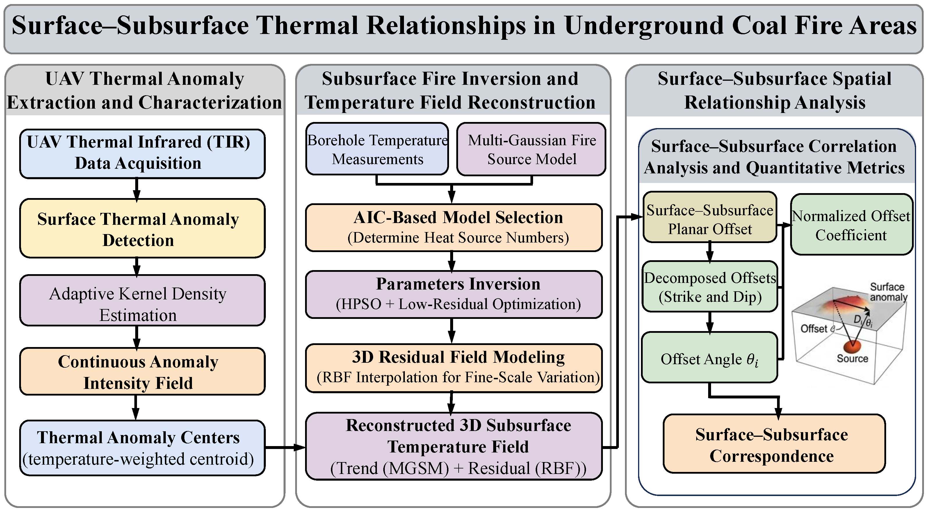
To address the above issues, this study investigates the spatial correspondence between surface thermal anomalies and subsurface fire sources by integrating UAV-based remote sensing with borehole temperature measurements. The main contributions of this study are twofold: (1) a quantitative framework is developed to characterize the spatial offset between surface thermal anomaly centers and subsurface fire sources, revealing that surface thermal signals are structurally controlled responses rather than vertical projections; and (2) a spatial-structure constrained method is proposed for reconstructing subsurface fire sources and three-dimensional temperature fields, enabling accurate identification of fire source locations and spatial thermal structures. The proposed approach is applied to the Sandaoba underground coal fire area in Miquan, Xinjiang, showing improved reconstruction performance compared with the tested methods and providing a potential reference for UAV-based coal fire interpretation and fire-control planning in complex coal fire environments.

2. Study Area and Datasets

2.1. Study Area

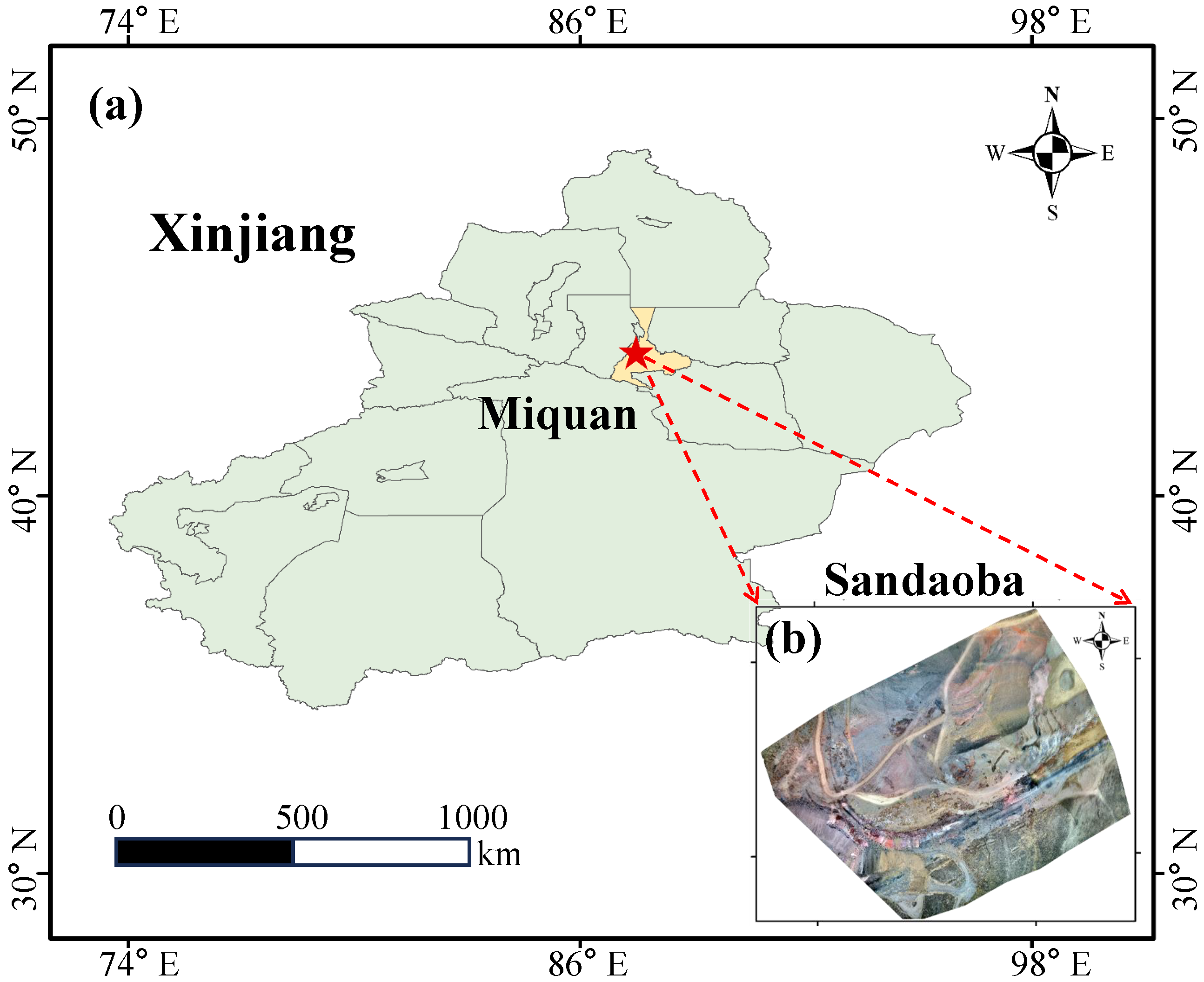
The study area is located in the Sandaoba coal fire zone in Miquan, Xinjiang, China, at approximately ${87}^{°}{48}^{\prime }{57}^{″}\mathrm{E}$ and ${43}^{°}{55}^{\prime }{52}^{″}\mathrm{N}$, about 34 km from Urumqi, as shown in Figure 1. It lies along the southern margin of the Junggar Basin and is characterized by a typical arid to semiarid continental climate, with low precipitation, high evaporation, and sparse vegetation. The area is situated in the piedmont zone of the Bogda Mountains, where the terrain decreases from southwest to northeast.

Geologically, the region is characterized by a monocline structure with steeply dipping coal seams of about $79$–${80}^{°}$. Multiple coal seams are developed, mainly composed of long-flame coal with low metamorphic maturity and a strong tendency for spontaneous combustion. Coal fire activity mainly occurs in several key seams, with a maximum combustion depth of about 191 m, showing coupled shallow to deep burning characteristics. The occurrence and evolution of coal fires are controlled by both geological conditions and long-term mining activities, which together provide favorable conditions for sustained combustion and progressive fire expansion.

2.2. UAV Thermal Infrared Data Acquisition

UAV data were acquired using a DJI M210 V2 platform equipped with a Zenmuse XT2 dual-sensor camera (DJI, Shenzhen, China), integrating both visible and thermal infrared sensors. The thermal infrared sensor operates in the $7.5$–$13.5\mathsf{\mu }\mathrm{m}$ spectral range with a thermal sensitivity better than 50 mK, while the visible sensor captures RGB imagery within the 400–$700\mathrm{nm}$ band. The camera provides two gain modes: a low-gain mode measuring $-40$–550 $°\mathrm{C}$ for high-temperature targets, and a high-gain mode measuring $-25$–135 $°\mathrm{C}$ for enhanced sensitivity. Given that the study area is dominated by subsurface coal fires with relatively subtle surface temperature variations, the high-gain mode was adopted to improve the detection of weak thermal anomalies.

The flight was conducted at an altitude of 80 m, with both forward and side overlaps set to 90% to ensure reliable image matching and three-dimensional reconstruction. Data acquisition took place on 6 November 2019. Under these conditions, the spatial resolutions of the visible and thermal infrared images were approximately 3.13 cm and 10.90 cm, respectively.

Image processing was performed using Pix4Dmapper, encompassing image alignment, geometric correction, three-dimensional reconstruction, and land surface temperature retrieval. Radiometric processing was conducted using the software’s built-in automatic workflow based on the sensor characteristics and image metadata. 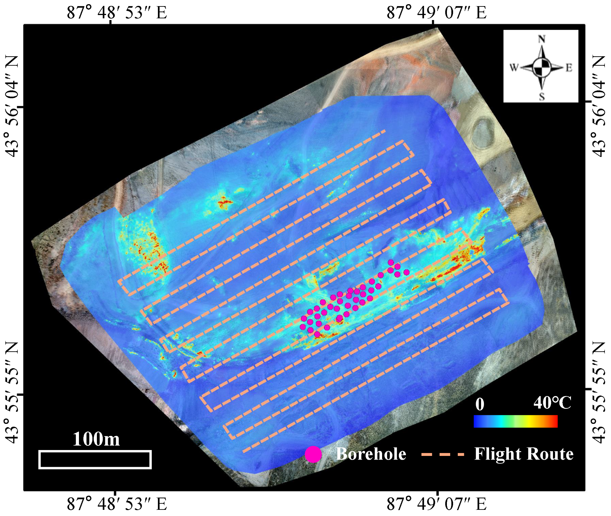The reliability of this UAV thermal infrared data and its processing procedure has been validated in previous coal-fire applications, showing strong agreement with ground measurements (with an $R^2$ of 0.99 and RMSE values generally around $1.4$ $°\mathrm{C}$ [11]. Since this study focuses on the relative spatial pattern and centroid positions of distinct surface thermal anomalies rather than improving absolute temperature retrieval accuracy, the derived temperature field is considered suitable for the surface-subsurface correspondence analysis. The resulting surface temperature distribution is shown in Figure 2.

2.3. Borehole Temperature Measurements

Borehole temperature data collected in October 2019 from the Sandaoba coal fire zone were used for fire source inversion and subsurface temperature field reconstruction. A total of 39 boreholes located near actively burning seams provided 370 valid temperature measurements, covering depths from the surface to approximately 85 m. The boreholes are relatively evenly distributed in plan view with a minimum spacing of about 10 m, and temperature measurements were recorded at approximately 5 m vertical intervals. It should be noted that the boreholes were concentrated in the core area with evident surface thermal anomalies and were not intended to uniformly cover the entire UAV survey area. Therefore, the subsequent subsurface temperature reconstruction and surface-subsurface offset analysis were restricted to the borehole-constrained active combustion zone.

3. Methods

To investigate the spatial correspondence between surface thermal anomalies and subsurface fire sources, this study first extracts surface thermal anomaly response centers from UAV thermal infrared data using an adaptive kernel density estimation method combined with temperature-weighted centroid calculation. Borehole temperature measurements are then used to reconstruct the three-dimensional subsurface temperature field and characterize fire-source structures using a multi-Gaussian source model coupled with radial basis function interpolation (MGSM–RBF). Based on these results, quantitative indicators, including dip-direction offset, strike-direction offset, and offset coefficients, are defined to characterize the spatial relationship between surface anomalies and subsurface fire sources. The overall workflow is illustrated in Figure 3.

3.1. Surface Thermal Anomaly Centers Extraction

3.1.1. Thermal Anomalies and Intensity Characterization Extraction

Surface thermal anomalies are identified from the UAV-derived temperature field $T(x,y)$ as indicators of potential subsurface fire activity. Following the coal-fire thermal anomaly extraction procedure established for UAV thermal infrared data [7,11], an initial thermal anomaly threshold was used to separate potential anomaly pixels from the background temperature field. The anomaly threshold is defined as

$$T_{th}=\mu +2\sigma$$

(1)

where $\mu$ and $\sigma$ represent the mean and standard deviation of temperature, respectively. Pixels satisfying $T(x,y)>T_{th}$ are classified as high-level thermal anomalies and used for subsequent analysis.

Since thermal anomalies extracted using a threshold are often spatially fragmented and discrete, an adaptive kernel density estimation (AKDE) approach is employed to construct a continuous intensity field [17,18]. A temperature-weighted kernel density function is defined as

$$I\left(\mathbf{s}\right)={\displaystyle \sum _{i=1}^n}{T}_i·{\displaystyle \frac{1}{h_i^2}}G\left({\displaystyle \frac{\parallel \mathbf{s}-{\mathbf{s}}_i\parallel }{h_i}}\right)$$

(2)

where ${\mathbf{s}}_i=(x_i,y_i)$ denotes the location of anomaly pixels, $T_i$ is the corresponding temperature, $G(·)$ is the kernel function and $h_i$ is the adaptive bandwidth at location ${\mathbf{s}}_i$. In this study, a Gaussian kernel is adopted

$$G\left(u\right)={\displaystyle \frac{1}{2\pi }}exp\left(-{\displaystyle \frac{1}{2}}{u}^2\right).$$

(3)

To account for spatial heterogeneity, the bandwidth is adjusted adaptively as

$$h_i=h_0{\lambda }_i,{\lambda }_i={\left({\displaystyle \frac{g}{\widehat{f}\left({\mathbf{s}}_i\right)}}\right)}^{1/2}$$

(4)

where $h_0$ is the global bandwidth, $\widehat{f}\left({\mathbf{s}}_i\right)$ is the pilot density estimate, and g is its geometric mean. This strategy enables smaller bandwidths in high-density regions to enhance local detail and larger bandwidths in sparse regions to maintain spatial continuity. To facilitate consistent interpretation, the intensity field is normalized to the range [0, 1].

3.1.2. Surface Thermal Anomaly Centers Determination

Based on the continuous intensity field, the center of each thermal anomaly is determined using an intensity-weighted centroid. For an anomaly region containing m pixels, with coordinates $(x_j,y_j)$ and normalized intensity $I_j^{\ast }$, the centroid is calculated as

$$x_c={\displaystyle \frac{{\sum }_{j=1}^m{I}_j^{\ast }{x}_j}{{\sum }_{j=1}^m{I}_j^{\ast }}},y_c={\displaystyle \frac{{\sum }_{j=1}^m{I}_j^{\ast }{y}_j}{{\sum }_{j=1}^m{I}_j^{\ast }}}.$$

(5)

This approach incorporates intensity weighting to account for internal spatial heterogeneity, providing a stable representation of the surface response to subsurface fire activity.

3.2. Subsurface Fire Source Inversion and Temperature Field Reconstruction

3.2.1. Multi-Gaussian Source Model Establishment

To characterize the spatial structure of subsurface coal fire sources and the corresponding temperature field, a quasi-steady assumption with anisotropic heat conduction is adopted. Rather than ideal point sources, subsurface coal fires are inherently finite combustion zones. Consequently, the temperature field is modeled as a superposition of multiple localized fire sources using a Multi-Gaussian Source Model (MGSM), where Gaussian functions are employed to capture their spatial boundaries and anisotropy [19].

Accordingly, the subsurface temperature field is expressed as

$$T\left(\mathbf{x}\right)=T_b+{\displaystyle \sum _{i=1}^B}{A}_{i}exp\left[-\left({\displaystyle \frac{{(x-x_i)}^2}{s_{x,i}^2}}+{\displaystyle \frac{{(y-y_i)}^2}{s_{y,i}^2}}+{\displaystyle \frac{{(z-z_i)}^2}{s_{z,i}^2}}\right)\right]$$

(6)

where $T_b$ is the background temperature, B is the number of fire sources, $A_i$ denotes the intensity of the i-th fire source, and $(x_i,y_i,z_i)$ represents its spatial location. The parameters $s_{x,i}$, $s_{y,i}$, $s_{z,i}$ describe the spatial diffusion scales along the three principal directions, reflecting anisotropic heat transfer.

3.2.2. Fire Source Number Determination

Subsurface coal fires typically exhibit multi-source thermal anomaly patterns. An insufficient number of fire sources may lead to underfitting and fail to capture dominant temperature variations. In contrast, an excessive number of parameters introduces redundancy, increasing model instability and the risk of overfitting. Therefore, determining an appropriate number of fire sources is essential for reliable modeling. In this study, the Akaike Information Criterion (AIC) is employed to balance model accuracy and complexity [20]. The AIC is defined as

$$AIC=nln\left({\displaystyle \frac{RSS}{n}}\right)+2p$$

(7)

where n is the number of observations, p is the number of model parameters, and $RSS={\sum }_{i=1}^n{(T_i-{\widehat{T}}_i)}^2$ denotes the residual sum of squares. For different candidate numbers of fire sources B, the model is fitted separately and the corresponding AIC values are computed. The optimal number of fire sources is then determined by

$$B^{\ast }=arg\underset{B}{min}AIC\left(B\right).$$

(8)

This approach enables an objective, quantitative selection of model complexity, thereby improving the stability and reliability of the inversion results.

3.2.3. Parameter Inversion and Low-Residual Optimization

The inversion of subsurface temperature fields involves a high-dimensional and strongly nonlinear parameter space, where the objective function is typically multimodal and prone to local optima. To improve global search capability and solution stability, a hybrid particle swarm optimization (HPSO) method is adopted for parameter inversion [21].

Within the HPSO framework, the velocity and position of each particle are updated as

$$\begin{array}{c}{v}_i^{(t+1)}=\omega v_i^{\left(t\right)}+c_1{r}_1\left(p_i^{best}-x_i^{\left(t\right)}\right)+c_2{r}_2\left(g^{best}-x_i^{\left(t\right)}\right)\\ x_i^{(t+1)}=x_i^{\left(t\right)}+v_i^{(t+1)}\end{array}$$

(9)

where $\omega$ is the inertia weight, $c_1$ and $c_2$ are acceleration coefficients, $r_1$ and $r_2$ are random variables, and $p_i^{best}$ and $g^{best}$ denote the personal and global best positions, respectively.

The inversion is formulated as a least-squares problem, where the objective function is defined as

$$J\left(\mathbf{p}\right)={\displaystyle \sum _{i=1}^N}{\left(T_i-T_{\mathrm{model}}({\mathbf{x}}_i;\mathbf{p})\right)}^2.$$

(10)

Although the general 3D Gaussian model allows independent scale parameters in three directions, the horizontal diffusion scales are assumed to be identical ($s_{x,i}$=$s_{y,i}$=$s_{xy,i}$) considering the similar spatial variation in the horizontal plane, while an independent vertical scale $s_{z,i}$ is retained to account for anisotropic heat transfer. This simplification reduces parameter redundancy and improves inversion stability.

The parameter set to be estimated is

$$\mathbf{p}={\{A_i,x_{0,i},y_{0,i},z_{0,i},s_{xy,i},s_{z,i}\}}_{i=1}^K\cup \left\{T_b\right\}$$

(11)

with a total dimension of $6K+1$.

To enhance robustness and mitigate the influence of local optima, a multi-start strategy HPSO is adopted. Parameter bounds were constrained by the spatial distribution of the boreholes, drilling depths and observed temperature limits. Within this bounded search space, multiple independent optimizations were executed using random initializations. In alignment with robust low-residual ensemble selection strategies [22,23], the top 5% of solutions with the lowest residuals were retained to construct a stable subset [24]. This strategy mitigates the risk of entrapment in a single local optimum while excluding unstable high-residual solutions.

To quantify the stability of the inversion results, the variance reduction ratio (VRR) is defined as

$$VRR=\left(1-{\displaystyle \frac{\mathrm{Var}\left(X_{elite}\right)}{\mathrm{Var}\left(X_{all}\right)}}\right)\times 100\%$$

(12)

where $X_{elite}$ and $X_{all}$ denote the low-residual subset and the full solution set, respectively.

3.2.4. Subsurface Temperature Field Reconstruction

Although the MGSM captures the dominant trend of the subsurface temperature field, complex thermal processes such as fracture-enhanced heat transfer and medium heterogeneity may lead to systematic deviations. To improve reconstruction accuracy, a radial basis function (RBF) model is introduced to compensate for these residuals [25].

The residual field is defined as the difference between observed temperatures and the MGSM-derived trend

$$R\left(\mathbf{x}\right)=T_{\mathrm{obs}}\left(\mathbf{x}\right)-T_{\mathrm{trend}}\left(\mathbf{x}\right).$$

(13)

To reconstruct the spatial structure of the residual field, an RBF interpolation model is adopted. The multiquadric basis function is used

$$T_{\mathrm{res}}\left(\mathbf{x}\right)={\displaystyle \sum _{i=1}^N}{w}_i\sqrt{\parallel \mathbf{x}-{\mathbf{x}}_i{\parallel }_W^2+{\epsilon }^2}$$

(14)

where $w_i$ denotes the weight coefficient associated with the i-th observation point, $\epsilon$ is the shape parameter that controls the smoothness of the RBF and is defined as $\epsilon =c{\overline{d}}_h$, where ${\overline{d}}_h$ denotes the average horizontal spacing of the boreholes and c is a dimensionless smoothing factor, and ${\parallel ·\parallel }_W$ represents the anisotropic weighted distance.

The final temperature field is obtained by combining the trend and residual components. This hybrid approach improves both reconstruction accuracy and spatial continuity.

3.3. Surface-Subsurface Spatial Relationship Analysis

3.3.1. Surface-Subsurface Spatial Offset Quantification

To quantify the spatial correspondence between subsurface fire sources and surface thermal anomaly centers, the horizontal offset distance is first calculated. The subsurface fire source center is denoted as $P_i=(x_i,y_i)$ and the corresponding surface anomaly center as $S_i=(x_i^{\prime },y_i^{\prime })$. The planar offset distance is defined as

$$D_i=\sqrt{{(x_i^{\prime }-x_i)}^2+{(y_i^{\prime }-y_i)}^2}.$$

(15)

To further characterize the directional dependence of thermal migration, the offset vector is decomposed into strike and dip components

$$d_{\mathrm{strike},i}=\Delta {\mathbf{d}}_i·{\mathbf{e}}_{\mathrm{strike}},d_{\mathrm{dip},i}=\Delta {\mathbf{d}}_i·{\mathbf{e}}_{\mathrm{dip}}$$

(16)

where ${\mathbf{e}}_{\mathrm{strike}}$ and ${\mathbf{e}}_{\mathrm{dip}}$ denote the unit vectors along the strike and dip directions of the coal seam, respectively. The relative contribution of these two components can be further described by the offset angle

$${\theta }_i=arctan\left({\displaystyle \frac{d_{\mathrm{dip},i}}{d_{\mathrm{strike},i}}}\right).$$

(17)

To eliminate the influence of burial depth differences among fire sources, a normalized offset coefficient is introduced

$${\eta }_i={\displaystyle \frac{D_i}{z_i}}$$

(18)

where $z_i$ is the burial depth of the subsurface fire source. Larger values of ${\eta }_i$ indicate stronger lateral migration of thermal anomalies relative to the source depth, reflecting a weaker vertical correspondence between surface response and subsurface fire location.

3.3.2. Surface-Subsurface Correspondence Establishment

In coal fire areas, the relationship between surface thermal anomalies and subsurface fire sources may involve one-to-one or many-to-one correspondences. To reduce subjectivity in the assignment, a rule-based interpretation procedure was adopted. First, each reconstructed subsurface fire source was linked to the nearest surface thermal anomaly center based on planar distance. This preliminary assignment was then refined by incorporating the spatial distribution patterns and intensity characteristics of thermal anomalies. Specifically, distance was used as the primary criterion, while anomaly morphology and intensity continuity were used as auxiliary criteria. If multiple subsurface fire sources were located beneath the same continuous high-intensity anomaly region and showed consistent spatial alignment with the surface anomaly pattern, a many-to-one correspondence was retained. The final correspondence was then reviewed using field observations and engineering interpretation experience. Through this procedure, a spatially and structurally consistent surface-subsurface correspondence is established.

4. Results

4.1. Surface Thermal Anomaly Centers Extraction and Analysis

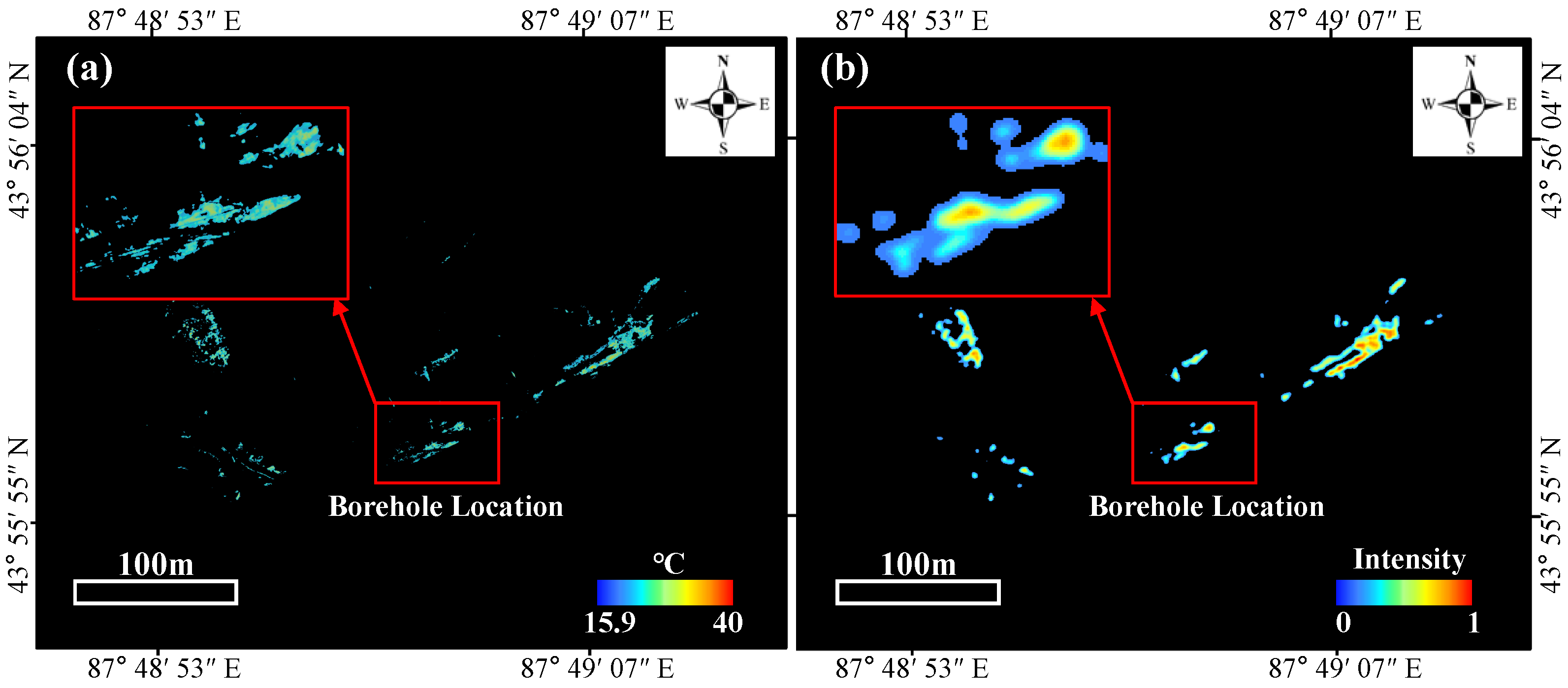
Using the $(\mu +2\sigma )$ criterion, the threshold for identifying thermal anomaly zones in the Sandaoba coal fire area was determined to be 15.9 °C. As shown in Figure 4a, high-level thermal anomalies exhibit a composite spatial pattern consisting of elongated bands and discrete patches.

At the regional scale, these anomalies are predominantly aligned along a near-linear trend that is broadly consistent with the orientation of coal seam occurrence. This pattern suggests that the surface thermal distribution is influenced by subsurface structural controls and heat transfer pathways. In addition, the anomaly bands are not completely isolated. Localized connections or transitions could be observed between adjacent zones, indicating possible thermal interactions among subsurface fire sources through fractures or conductive pathways.

At a finer scale, the high-level anomaly regions display noticeable internal heterogeneity, with multiple localized hotspots occurring within individual patches. This multi-core pattern suggests that a single surface anomaly may correspond to multiple subsurface fire sources or to heat transport through several pathways. It therefore provides a basis for subsequent surface-subsurface spatial analysis.

Based on the extracted thermal anomaly regions, an adaptive kernel density–weighted intensity field was constructed. Regions with normalized intensity values greater than 0.25 were identified as the primary thermal anomaly areas. This threshold was selected based on engineering interpretation experience and multi-threshold trial segmentation of the normalized intensity field. A lower threshold tended to include weak background responses and transitional edges, resulting in an overly large anomaly region and unstable extraction of core response centers. In contrast, a higher threshold caused excessive shrinkage and fragmentation of the anomaly regions, which weakened the continuity of the main thermal response. Therefore, a normalized intensity threshold of 0.25 was adopted as a balanced value to preserve the dominant continuous anomaly structures while suppressing low-intensity background disturbances.

As shown in Figure 4b, two dominant surface thermal anomaly centers are identified in the study area. The northeastern anomaly forms a relatively compact, near-circular to irregular patch, with a concentrated high-intensity core and a coherent spatial structure. In contrast, the southwestern anomaly exhibits an elongated, elliptical pattern aligned with the principal orientation of anomaly distribution, with a more dispersed structure and a larger spatial extent.

Overall, the surface thermal anomalies show a combination of compact clusters and elongated band-like features. The differences in morphology and scale among these anomalies reflect spatial variability in subsurface thermal processes and support the analysis of surface-subsurface spatial relationships.

4.2. Underground Fire Source Location Inversion

4.2.1. Borehole Data Distribution Characteristics

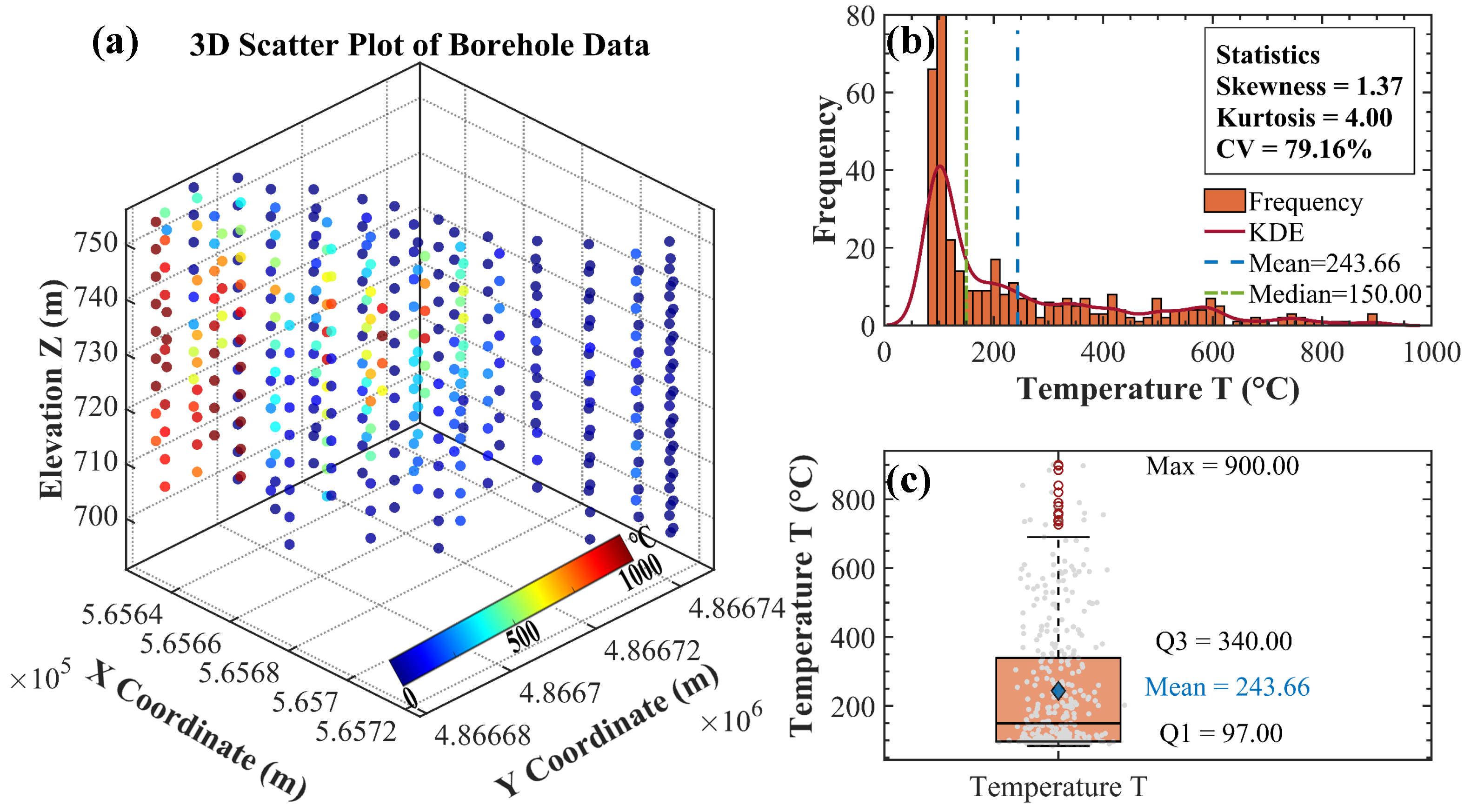
Based on the histogram and box plot in Figure 5, the 370 borehole temperature samples exhibit clear heterogeneity and a right-skewed distribution. The mean and median are $243.6$ $°\mathrm{C}$ and $150.0$ $°\mathrm{C}$, respectively, indicating that the distribution is influenced by high-temperature values. The standard deviation is $192.9$ $°\mathrm{C}$, with a coefficient of variation (CV) of 79.16%, suggesting a high level of dispersion in the temperature data.

In terms of distribution shape, the data show a pronounced right skew with a long tail toward high values. Most samples are concentrated within the range of $80.0$–$150.0$ $°\mathrm{C}$, with a peak near $100.0$ $°\mathrm{C}$. The skewness is 1.37 and the kurtosis is 4.00, indicating a positively skewed distribution with a relatively concentrated central range and extended high-value tail. The box plot shows that the median is closer to the lower quartile, and the upper whisker is longer with several high-value outliers. Overall, the temperature data reflect spatial heterogeneity and suggest the presence of localized high-temperature zones within a broader background temperature field, providing a basis for multi-source fire inversion.

4.2.2. Fire Source Number Determination and Analysis

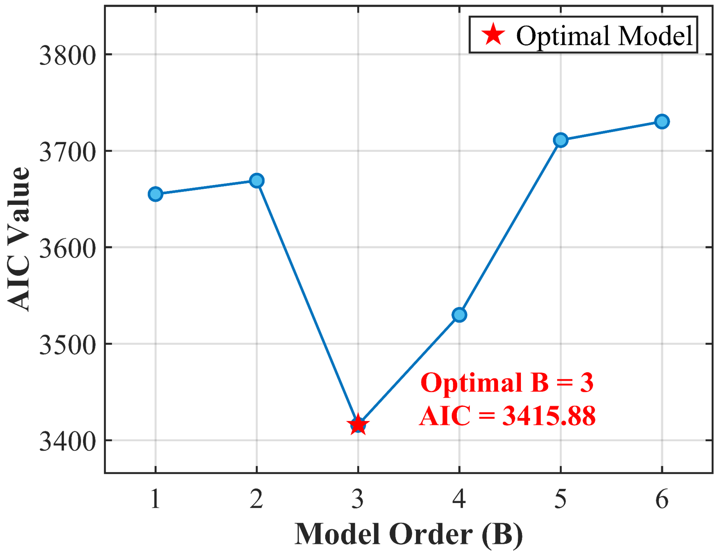
Considering the limited spatial extent of the study area and the relatively dense distribution of boreholes, the number of subsurface fire sources is assumed to be finite. As the number of model parameters increases with the number of fire sources, excessive sources may lead to increased model complexity and overfitting. To balance model complexity and fitting performance, the maximum number of candidate fire sources was set to $B_{max}=6$, and the AIC was used to evaluate models with different source numbers, as shown in Figure 6.

The AIC value decreases significantly as the number of fire sources increases from 1 to 3, indicating improved model fit. The minimum AIC is achieved at $B=3$, suggesting an optimal balance between goodness of fit and model complexity. For $B>3$, the AIC shows no further improvement, indicating limited benefit from additional parameters. Therefore, the optimal number of fire sources is determined as 3, and the corresponding model is adopted for subsequent inversion and analysis.

4.2.3. Parameter Configuration and Inversion Stability Analysis

To keep the HPSO search within a physically meaningful domain and reduce unstable local optima, bounded constraints were imposed on the MGSM parameters. To reduce boundary truncation effects, the source-location parameters were allowed to extend beyond the normalized model domain, with a search range of $[-50, 150]$. The source intensity A was constrained to $[100, 1500] °\mathrm{C}$, based on the observed borehole temperatures and expected coal-fire conditions. The horizontal and vertical diffusion scales were constrained to $[5, 50]$ in normalized units, allowing the model to represent both compact local fire sources and more diffuse thermal anomaly zones.

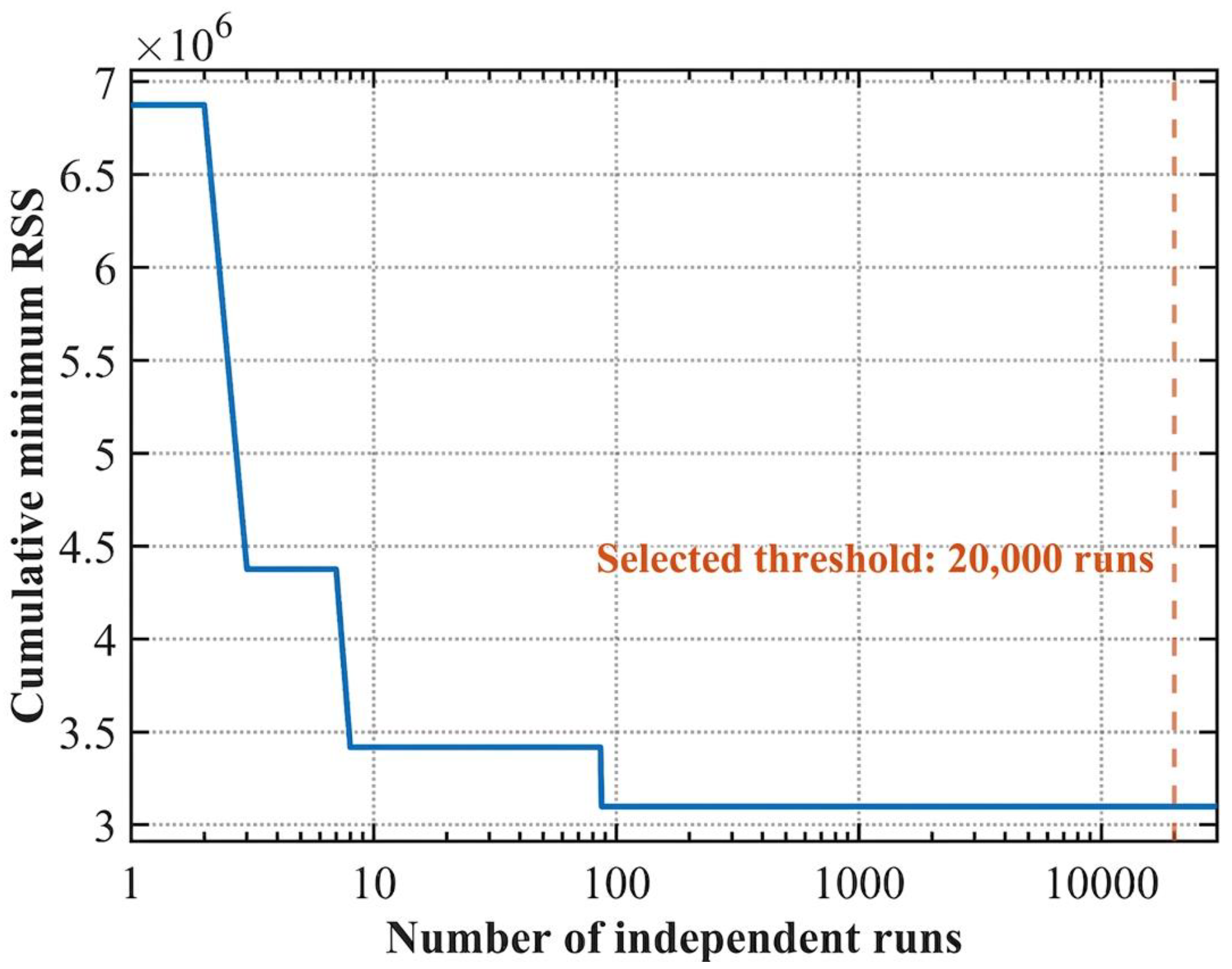
A multi-start strategy with 20,000 independent HPSO runs was used to reduce the influence of random initialization and local optima. This number was not treated as a universal empirical value, but was selected based on the stability of the cumulative minimum residual. As shown in Figure 7, the cumulative minimum RSS decreased rapidly in the early stage and became nearly stable after approximately ${10}^2$ runs. Although the best residual stabilized early, 20,000 runs provided sufficient sampling of the high-dimensional parameter space for low-residual solution selection and subsequent stability analysis. The stable clustering of the low-residual solutions further indicates that this run number was sufficient for robust fire-source inversion and parameter estimation.

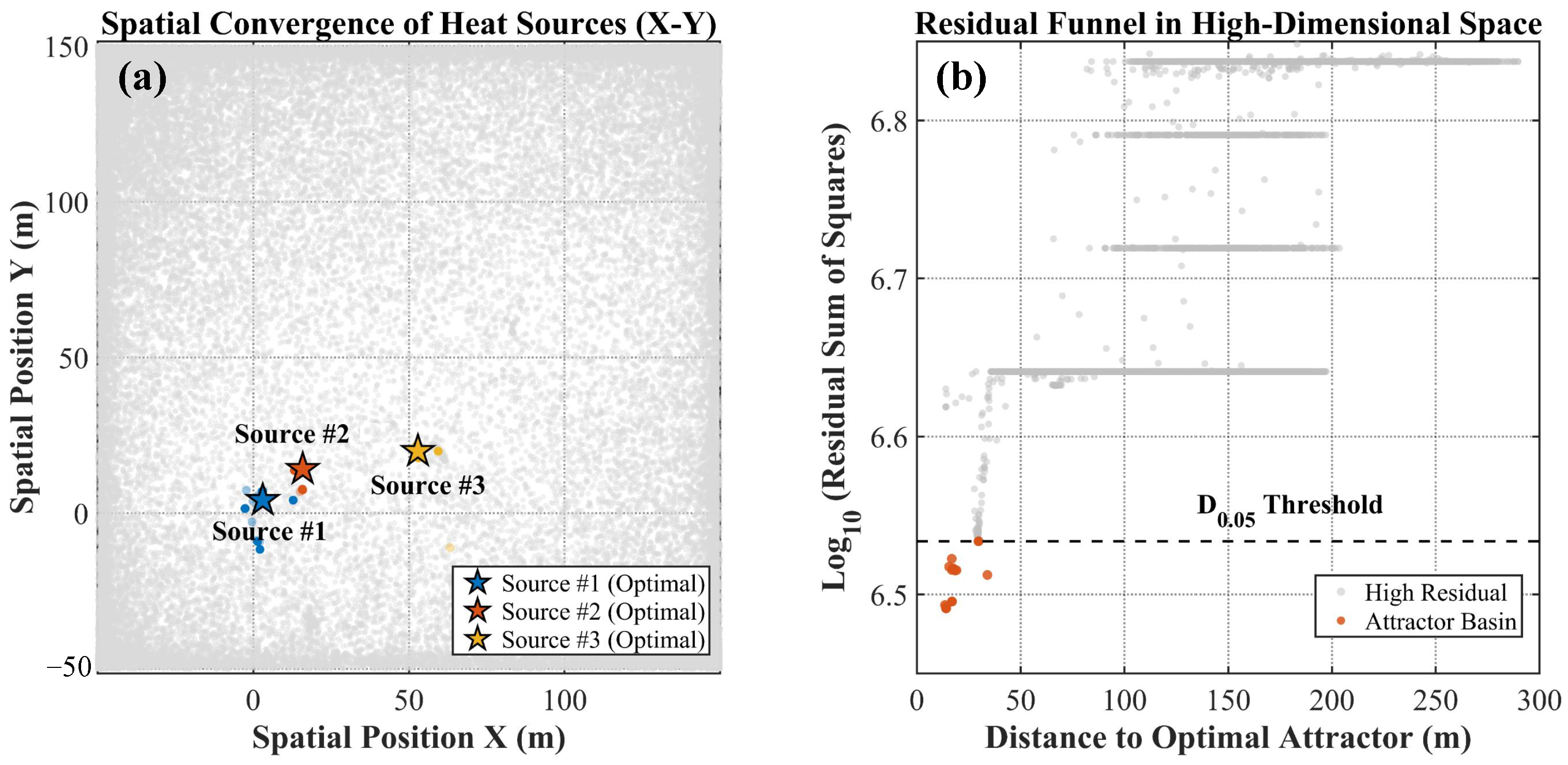
The residual distribution exhibits a typical funnel-shaped pattern (Figure 8), with a wide spread at high residual levels and convergence toward a limited low-residual region. Most solutions remain in higher-residual regions, while only a small proportion converges to low-residual solutions, indicating a nonlinear parameter space with a stable solution region. The lowest 5% of solutions are selected to form a low-residual subset, within which the VRR of the three fire sources in the horizontal plane reach 94.83%, 87.34%, and 99.42%, respectively. These results indicate reduced parameter uncertainty and clear spatial clustering of solutions. Overall, although the solution space is complex, a limited number of parameter configurations are consistently supported by the data, suggesting stable and well-constrained inversion results.

4.2.4. Inverted Fire Source Parameters Characteristics

Based on the low-residual subset obtained from multi-start inversion, stable parameter estimates were derived using median statistics, and their variability was evaluated using standard deviation (Std) and CV, as summarized in

Table 1. Statistical results of multi-fire source parameter inversion.

Source ID	Parameter	Inversion Estimate (Median ± Std)	Relative Uncertainty (CV%)
Source #1	Position x (m)	$3.05\pm 5.97$	–
	Position y (m)	$4.16\pm 6.59$	–
	Position z (m)	$46.23\pm 8.77$	–
	Intensity A ($°$C)	$1096.93\pm 171.89$	15.67%
	Horizontal scale $s_h$ (m)	$11.32\pm 4.36$	38.2%
	Vertical scale $s_z$ (m)	$24.37\pm 0.54$	2.21%
Source #2	Position x (m)	$15.90\pm 7.71$	–
	Position y (m)	$14.15\pm 7.67$	–
	Position z (m)	$57.36\pm 6.04$	–
	Intensity A ($°$C)	$847.85\pm 121.75$	15.3%
	Horizontal scale $s_h$ (m)	$4.41\pm 1.93$	43.74%
	Vertical scale $s_z$ (m)	$18.99\pm 3.64$	19.17%
Source #3	Position x (m)	$52.91\pm 3.28$	–
	Position y (m)	$19.90\pm 1.76$	–
	Position z (m)	$39.30\pm 1.35$	–
	Intensity A ($°$C)	$467.71\pm 78.25$	16.73%
	Horizontal scale $s_h$ (m)	$12.64\pm 1.97$	15.59%
	Vertical scale $s_z$ (m)	$15.98\pm 2.09$	13.08%

.

For spatial location parameters, Std is used to assess absolute variability. The standard deviations of the three fire sources range from $1.76$–$7.71\mathrm{m}$ in the horizontal directions and from $1.35$–$8.77\mathrm{m}$ in depth, indicating consistent spatial convergence under repeated random initializations. The three sources remain clearly separated, with no evident overlap or positional drift, suggesting that the inversion can reliably distinguish multiple fire sources.

For shape-related parameters, including source intensity and spatial scales, CV is used to evaluate relative uncertainty. The CV values for source intensity range from 15% to 17%, indicating moderate variability. Higher CV values are observed for some horizontal scale parameters, such as 38.2% for source #1 and 43.74% for source #2. However, these values are partly influenced by relatively small parameter magnitudes, for example, a horizontal scale of 4.41 m with a standard deviation of 1.93 m for source #2. Overall, the parameter estimates exhibit stable clustering behavior, indicating that the inversion results are well constrained by the available data despite the inherent non-uniqueness of the problem.

4.3. Subsurface Temperature Field Reconstruction and Analysis

4.3.1. RBF-Based Residual Correction and Temperature Field Reconstruction

To refine localized thermal anomalies not captured by the MGSM trend, RBF interpolation is applied to model the residual field. An anisotropic distance metric is introduced to account for stronger vertical temperature gradients, with the vertical weighting coefficient set to 6.0 based on temperature-weighted spatial dispersion. The smoothing parameter is adaptively defined as 0.6 times the average horizontal borehole spacing, and a small ridge regularization term on the order of ${10}^{-4}$ is introduced to enhance numerical stability.

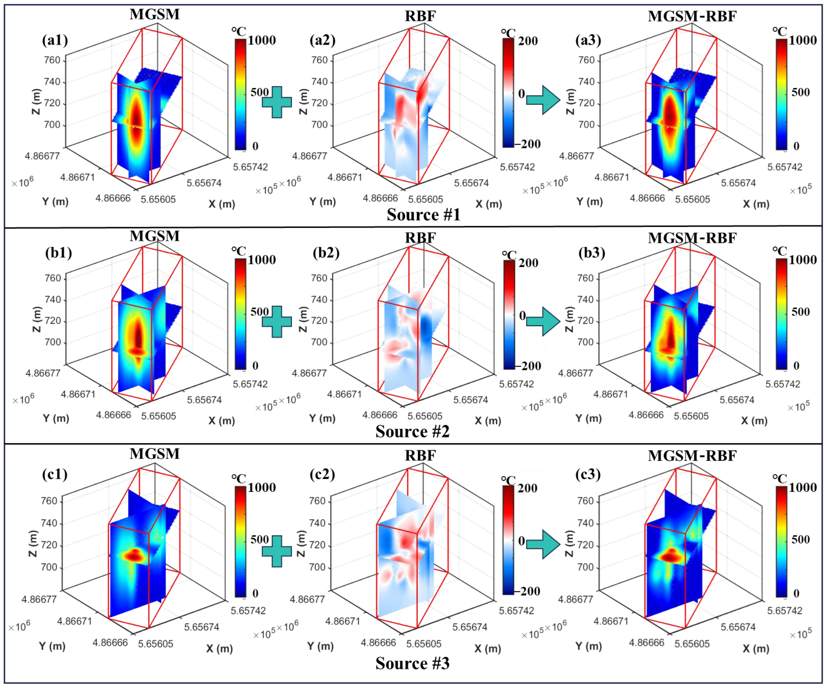
Figure 9 presents the reconstructed three-dimensional subsurface temperature field obtained by combining the MGSM trend and RBF residual correction. The MGSM trend field shows smooth and continuous ellipsoidal temperature distributions, with peak temperatures approaching 1000 $°\mathrm{C}$, reflecting the large-scale conductive heat diffusion pattern. In contrast, the RBF residual field ranges approximately from $-200$–200 $°\mathrm{C}$ and exhibits clear spatial heterogeneity, with localized positive and negative anomalies distributed around the fire source centers. After residual correction, the reconstructed temperature field retains the overall structure of the MGSM trend while introducing localized variations, particularly in the lower and peripheral regions of the fire sources, where more complex spatial features can be observed. These results indicate that the RBF-based correction enhances the representation of local thermal variability and improves the agreement with observed temperature patterns.

4.3.2. Fire Source Vertical Profiles Analysis

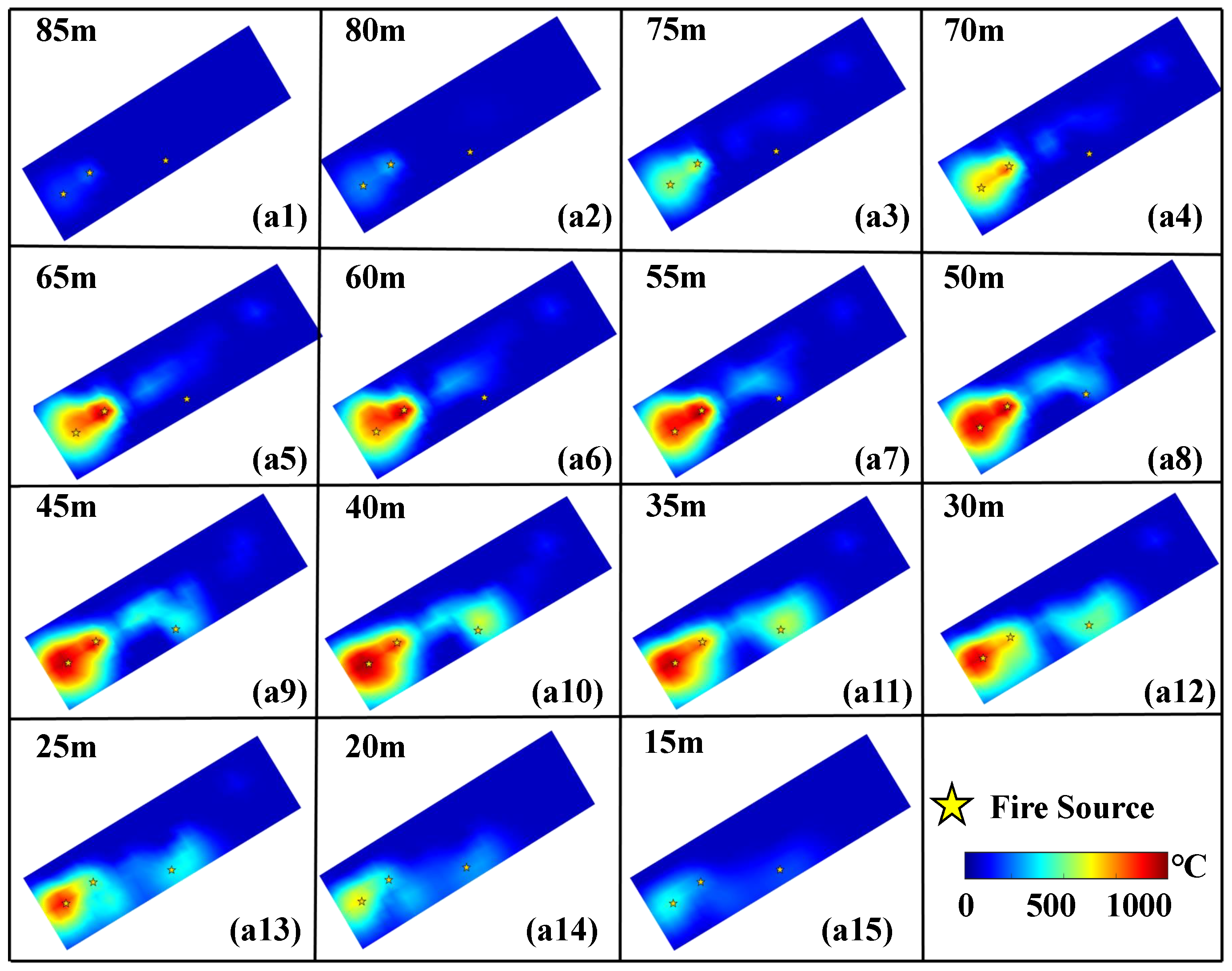
It could be seen from Figure 10 that horizontal temperature slices at depths from 15–85 m reveal a clear vertical evolution pattern of the subsurface thermal field. At depths of 80–85 m, temperatures remain at background levels, with only weak and localized anomalies near the western fire source. As depth decreases to 60–75 m, thermal anomalies intensify, with a stable high-temperature core forming in the western region and secondary anomalies emerging in the central and eastern areas. The most pronounced development occurs at depths of 30–55 m, where high-temperature zones expand and become interconnected, forming a continuous thermal structure. At shallower depths of 15–25 m, the anomalies begin to contract, and connectivity weakens.

The results indicate a vertically stratified thermal structure characterized by weak deep responses, a strongly developed intermediate combustion zone, and a shallow attenuation layer. The main combustion activity is concentrated at depths of approximately 30–55 m, where multiple fire sources interact and form a connected thermal system. This layered structure provides a basis for identifying combustion zones and determining target depths for fire control.

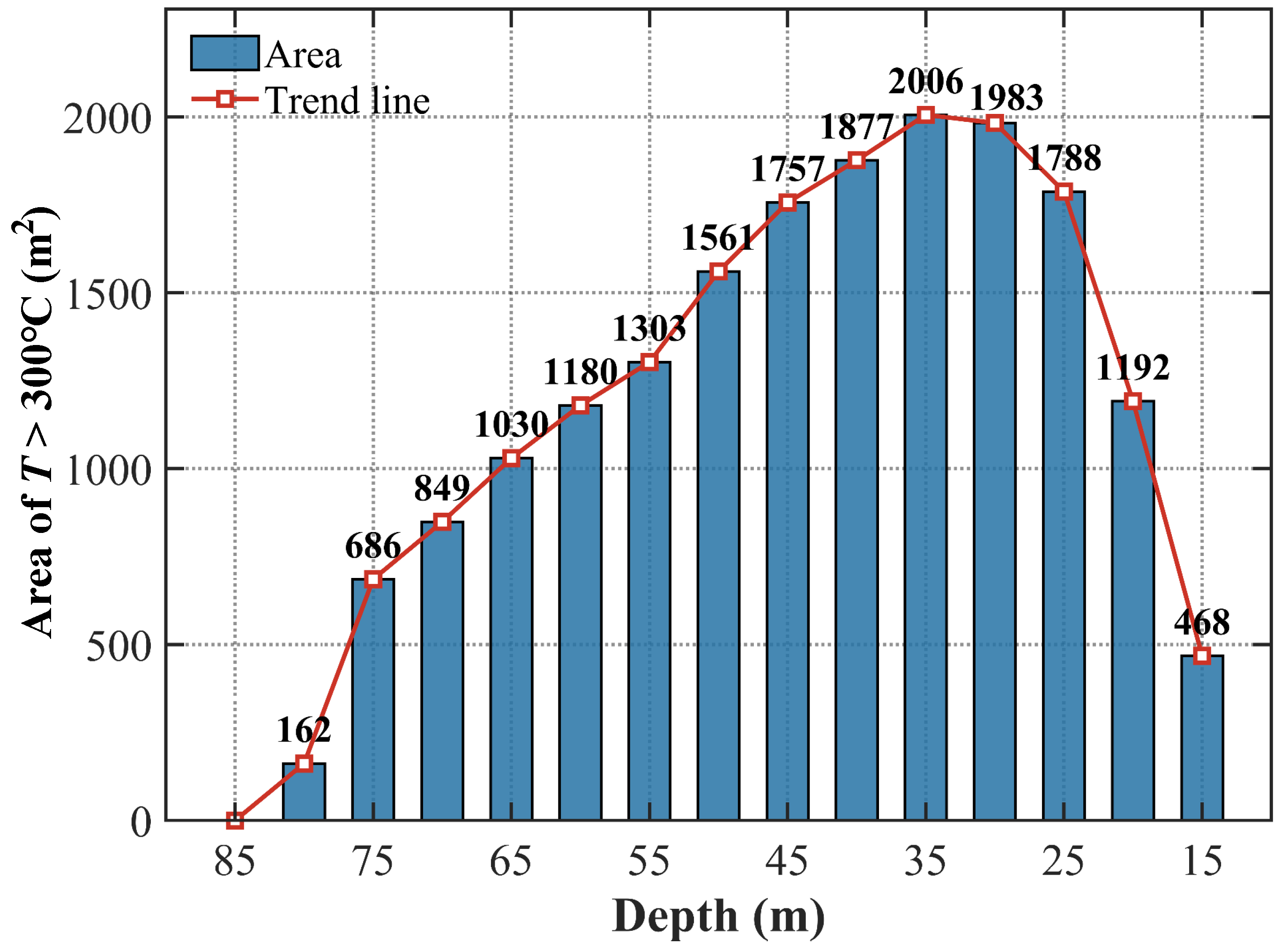
To quantitatively characterize the development of high-temperature combustion zones at different depths, $300 °\mathrm{C}$ was selected as the threshold for area calculation. Previous studies have commonly regarded this temperature range as a critical boundary between low-temperature oxidation and more intense pyrolysis or combustion activity in coal spontaneous combustion [26,27]. The area with $T>300 °\mathrm{C}$ was therefore calculated for each horizontal slice to describe the vertical evolution of the reconstructed subsurface temperature field, as shown in Figure 11.

The results show that the area with $T>300 °\mathrm{C}$ first increases and then decreases with decreasing depth. At the deep levels of 80–85 m, high-temperature zones are poorly developed, with only a localized anomaly of approximately 162 ${\mathrm{m}}^2$ at 80 m. As the depth decreases to 60–75 m, the high-temperature area increases from 686 ${\mathrm{m}}^2$ to 1180 ${\mathrm{m}}^2$, indicating that subsurface thermal anomalies gradually intensify and develop into a multi-center structure. At depths of 30–55 m, the high-temperature area further expands and remains at a high level, reaching a maximum of 2006 ${\mathrm{m}}^2$ at 35 m and remaining at 1983 ${\mathrm{m}}^2$ at 30 m. This indicates that the main combustion activity is concentrated within this depth interval. When the depth further decreases to 15–25 m, the high-temperature area rapidly decreases from 1788 ${\mathrm{m}}^2$ to 468 ${\mathrm{m}}^2$, reflecting the attenuation of shallow thermal anomalies. These quantitative results further support the layered interpretation described above, namely a vertical thermal structure characterized by weak deep responses, a strongly developed intermediate combustion zone, and shallow attenuation.

4.4. Spatial Offset Characteristics

4.4.1. Spatial Offset Characteristics Between Subsurface Fire Sources and Surface Thermal Centers

To quantitatively characterize the spatial relationship between subsurface fire sources and surface thermal anomaly centers, planar offsets were calculated based on three identified subsurface fire sources and two surface response centers.

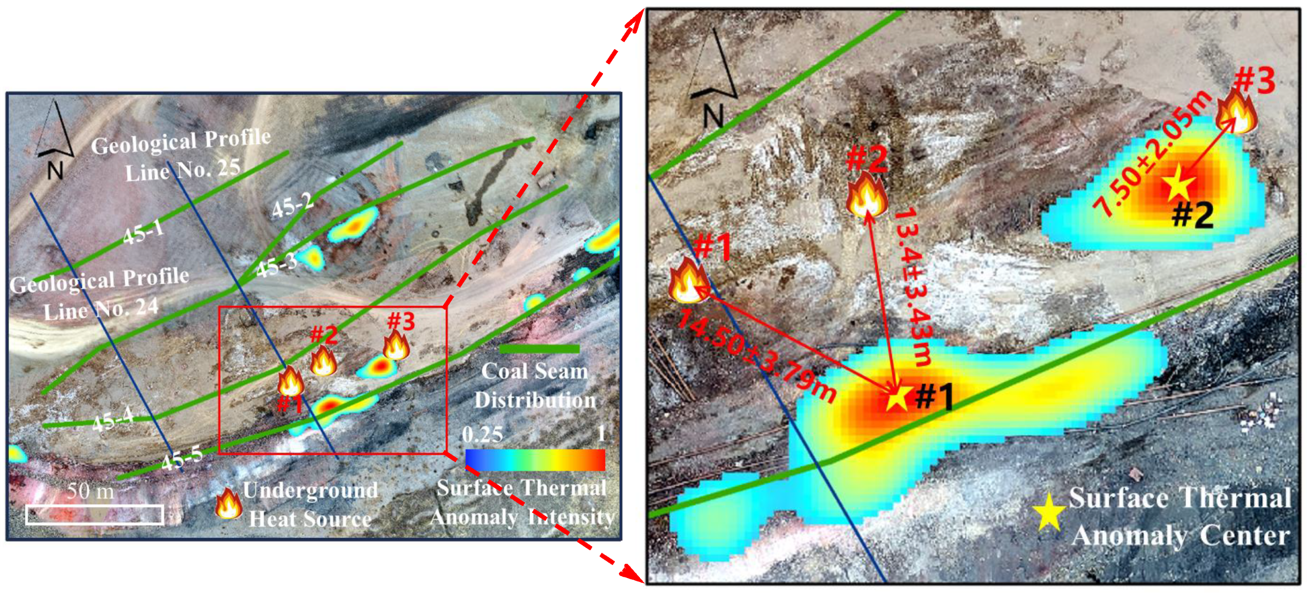
As shown in Figure 12, the main combustion occurs between the 45-5 and 45-4 coal seams, which dip steeply toward the northwest at approximately 80°. Under this geological setting, heat transfer from subsurface sources to the surface is constrained by coal seam structure, resulting in directional offsets between surface anomalies and subsurface fire sources. Therefore, the spatial relationship cannot be adequately characterized by Euclidean distance alone. To better capture the structural control on heat transfer, the planar offset was further decomposed into strike-direction and dip-direction components.

The surface thermal anomalies in Sandaoba coal fire area could be divided into two relatively independent response units. The southwestern anomaly is characterized by an elongated high-intensity zone broadly aligned with the coal seam distribution, whereas the northeastern anomaly appears as a more compact patch. Therefore, the surface-subsurface correspondence was not determined solely by the nearest planar distance, but was interpreted by jointly considering planar distance, anomaly intensity continuity, anomaly morphology, and coal seam distribution. Specifically, Fire Sources #1 and #2 are both located within the influence range of the southwestern continuous band-like thermal anomaly, and their spatial positions and offset directions are consistent with the extension of this anomaly zone. They were therefore assigned to Surface Center #1, indicating a many-to-one correspondence between multiple subsurface sources and a single surface response center. In contrast, Fire Source #3 is located close to the relatively independent northeastern thermal anomaly patch and is nearer to Surface Center #2. It was therefore assigned to Surface Center #2. To assess the influence of fire-source location uncertainty on the offset metrics, direct uncertainty propagation was performed using the lowest 5% low-residual solutions. For each retained solution, the offset metrics were recalculated and the probable error $PE=0.6745\sigma$ was used to express the uncertainty [28,29]. The resulting offset measurements are summarized in

Table 2. Statistics of spatial offset parameters between underground fire sources and surface thermal anomaly response centers.

Source ID	Depth H (m)	Dip Dist. ${\mathit{L}}_{\mathit{d}}$ (m)	Strike Dist. ${\mathit{L}}_{\mathit{s}}$ (m)	Horiz. Dist. ${\mathit{L}}_{\mathit{h}}$ (m)	Offset Angle $\mathit{\theta }$ ($°$)	Offset Coeff. ${\mathit{\eta }}_{\mathit{i}}$
Source #1	$46.23\pm 2.13$	$12.40\pm 1.15$	$7.50\pm 4.09$	$14.50\pm 3.79$	$58.8\pm 19.6$	$0.31\pm 0.08$
Source #2	$57.36\pm 4.09$	$12.20\pm 0.43$	$5.50\pm 4.77$	$13.40\pm 3.43$	$65.7\pm 15.7$	$0.23\pm 0.06$
Source #3	$39.30\pm 0.91$	$1.10\pm 0.57$	$7.40\pm 2.05$	$7.50\pm 2.05$	$8.5\pm 1.0$	$0.19\pm 0.05$

and Figure 12.

The results indicate that, in underground coal fire settings, surface thermal anomaly centers do not correspond to the vertical projections of subsurface fire sources, but instead exhibit distinct horizontal offsets. After uncertainty propagation, the horizontal offset distances of the three fire sources are $14.50\pm 3.79$ m, $13.40\pm 3.43$ m, and $7.50\pm 2.05$ m, respectively, indicating non-vertical offsets from several meters to more than ten meters between surface thermal anomalies and subsurface fire sources. The corresponding offset coefficients are $0.31\pm 0.08$, $0.23\pm 0.06$, and $0.19\pm 0.05$, suggesting that the horizontal offset is generally approximately one-fifth to one-third of the combustion depth, although this scaling relationship contains certain uncertainty.

The directional decomposition shows that the dip-direction offsets of Source #1 and Source #2 are $12.40\pm 1.15$ m and $12.20\pm 0.42$ m, respectively, both of which are larger than their corresponding strike-direction offsets. This indicates that the surface thermal responses of these two sources mainly migrate along the dip direction of the coal seam. The relatively larger uncertainty in the strike-direction offsets reflects stronger positional dispersion along the strike direction. In contrast, Source #3 has a strike-direction offset of $7.40\pm 2.05$ m and a much smaller dip-direction offset of $1.10\pm 0.57$ m, showing a strike-dominated offset pattern. This difference suggests that local heat transfer may be affected by multi-source superposition or fracture-controlled pathways.

The offset angles further reflect the directional differences in the surface–subsurface spatial relationship. The offset angles of Source #1 and Source #2 are $58.8°\pm 19.6°$ and $65.7°\pm 15.7°$, respectively, indicating a generally dip-dominated offset pattern, whereas Source #3 has an offset angle of $8.5°\pm 1.0°$, indicating a strike-dominated pattern. Since the offset angle is calculated from the ratio between the dip and strike direction offset components, its uncertainty can be amplified when one component is relatively small or has relatively large variability. Therefore, the combined interpretation of offset distance, directional decomposition, and propagated uncertainty provides a more complete characterization of the surface-subsurface thermal response relationship than a single angular value.

Overall, after considering the uncertainty in fire-source location inversion, a stable non-vertical correspondence remains evident between surface thermal anomalies and subsurface fire sources. The horizontal offset magnitude shows a certain scaling relationship with combustion depth, while the offset direction and local variations are jointly controlled by coal seam geometry, fracture pathways, and multi-source thermal-field superposition.

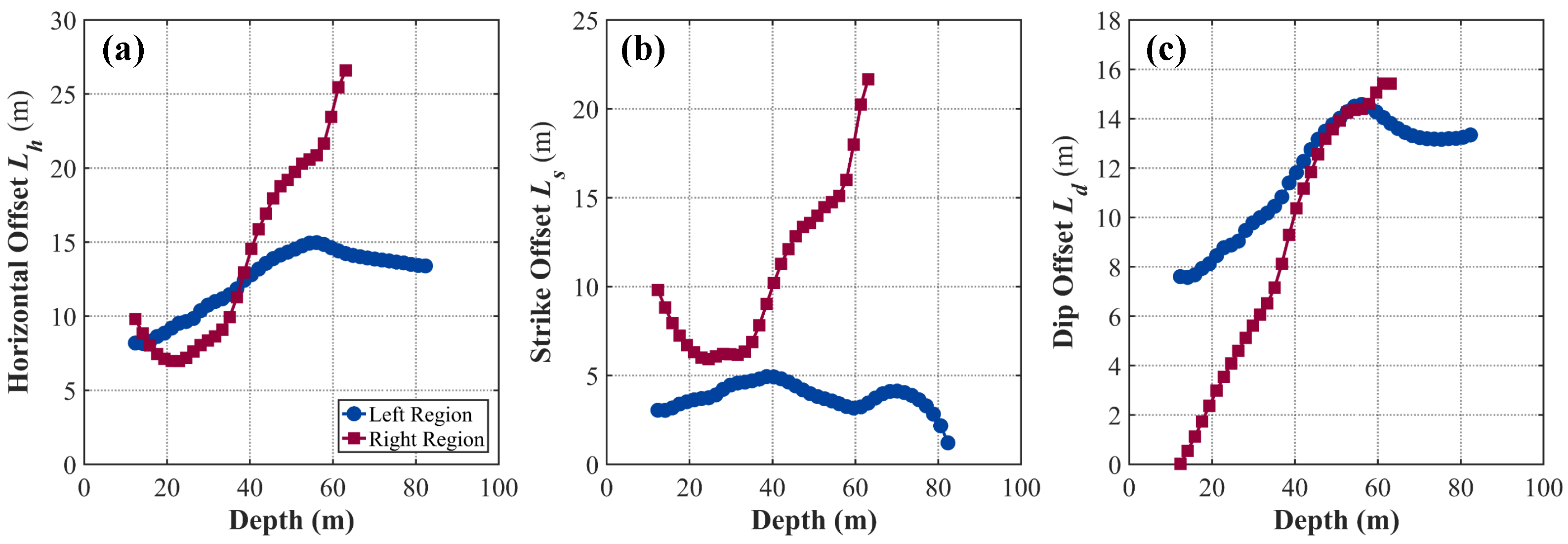
4.4.2. Spatial Offset Characteristics Between Subsurface Thermal Anomaly Centers at Different Depths and Surface Thermal Centers

To investigate the offset relationship between subsurface thermal anomaly centers at different depths and surface thermal anomaly centers, the three-dimensional temperature field was stratified at 2 m intervals. As discussed in Section 4.3.2, high-temperature zones exceeding $300 °\mathrm{C}$ were extracted to isolate intense combustion regions. Considering the close proximity and partial overlap of Fire Sources #1 and #2, a combined temperature-weighted centroid was calculated, whereas Fire Source #3, being spatially isolated, was treated independently. The resulting depth-dependent thermal anomaly centers were then compared with surface observations, as shown in Figure 13.

Synthesizing the offset parameters, the spatial relationship between subsurface thermal anomaly centers at different depths and surface thermal anomaly centers shows clear depth-dependent and directionally coupled characteristics. In the deep zone above 60 m, Fire Source #3 has negligible influence due to its shallow burial, while Fire Sources #1 and #2 exhibit limited offset variations within 0–3 m, indicating stable heat conduction at depth. As depth decreases above 60 m, multi-source superposition becomes more pronounced, leading to increasingly complex offset patterns.

For Fire Source #3, the horizontal offset decreases rapidly from approximately 25 m to 8 m within the 20–60 m interval. This reduction is attributed to the influence of the stronger thermal fields of Fire Sources #1 and #2, which induce a lateral shift of the anomaly center. As the depth approaches its main combustion level at around 39 m, the influence of Fire Source #3 strengthens, causing the anomaly center to gradually return toward its own projection.

In contrast, Fire Sources #1 and #2 exhibit relatively stable offsets along the dip direction, with minimum distances of about 6 m. Overall, the results indicate that surface thermal anomaly centers are governed by the combined effects of multiple subsurface fire sources and coal seam structure.

5. Discussion

5.1. Sensitivity of Surface Thermal Anomaly Center Extraction

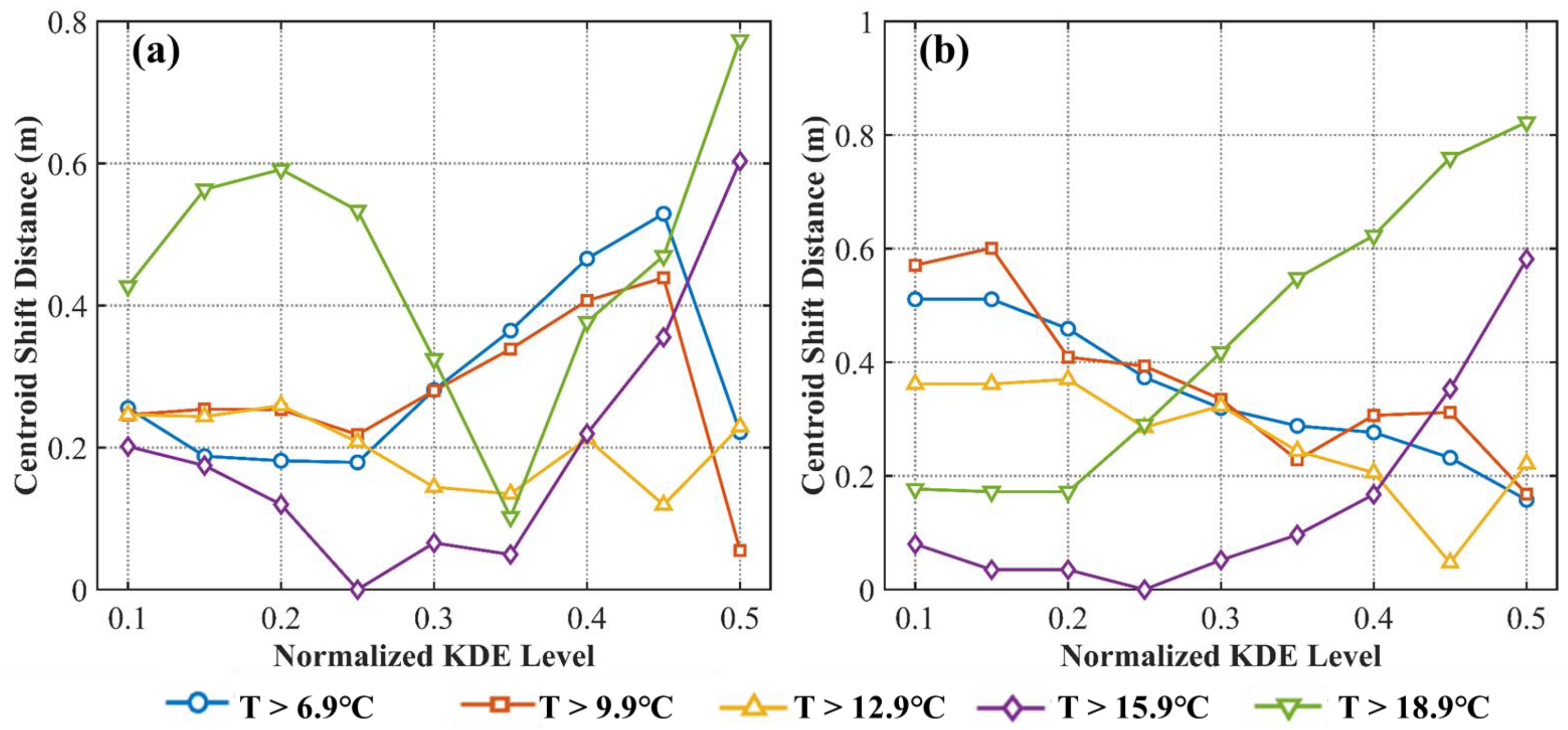
To examine the influence of threshold selection on the extracted surface thermal anomaly centers, a center-stability analysis was conducted using the initial setting of $T>15.9 °\mathrm{C}$ and a normalized KDE level of 0.25 as the reference. Different temperature thresholds and normalized KDE levels were then tested, and the displacement of the two extracted surface thermal anomaly centers relative to the reference centers was calculated, as shown in Figure 14. Considering the right-skewed distribution of surface temperature in coal fire areas, a single mean-plus-standard-deviation threshold may miss some medium- to low-intensity thermal responses. Therefore, the temperature thresholds were set from $6.9 °\mathrm{C}$ to $18.9 °\mathrm{C}$ at intervals of 3$°\mathrm{C}$, where $6.9 °\mathrm{C}$ represents the mean background temperature on the observation date. The normalized KDE level was varied from 0.1 to 0.5 to examine the influence of different core-anomaly extraction levels.

The results show that the displacement of both surface thermal anomaly centers remained within 1 m under all tested threshold combinations. For Surface Center #1, the centroid shift was generally less than 0.6 m under most temperature and KDE-level settings, with only a slight increase at the highest KDE level. For Surface Center #2, the displacement also remained below 1 m, although a gradual increase was observed when the KDE level exceeded 0.35, especially under the higher temperature threshold, indicating that increasing the KDE level causes the extracted anomaly region to shrink toward the high-intensity core, leading to a slightly larger centroid shift. Nevertheless, the overall displacement range is much smaller than the surface–subsurface offset distances. The results demonstrate that the selected threshold combination provides stable surface thermal anomaly centers.

5.2. Comparison of Prediction Accuracy Metrics for Different Methods Under Spatially Buffered Cross-Validation

To evaluate the reconstruction performance, nine methods were compared, including MGSM–RBF, MGSM, polynomial interpolation (PI), inverse distance weighting (IDW), ordinary kriging (OK), natural neighbor interpolation (NNI), isotropic MGSM-RBF, anisotropic Gaussian process regression (GP-Aniso), and isotropic Gaussian process regression (GP-Iso). GP-Aniso used an automatic relevance determination squared-exponential kernel to allow direction-dependent length scales, whereas GP-Iso used a single isotropic squared-exponential kernel [30].

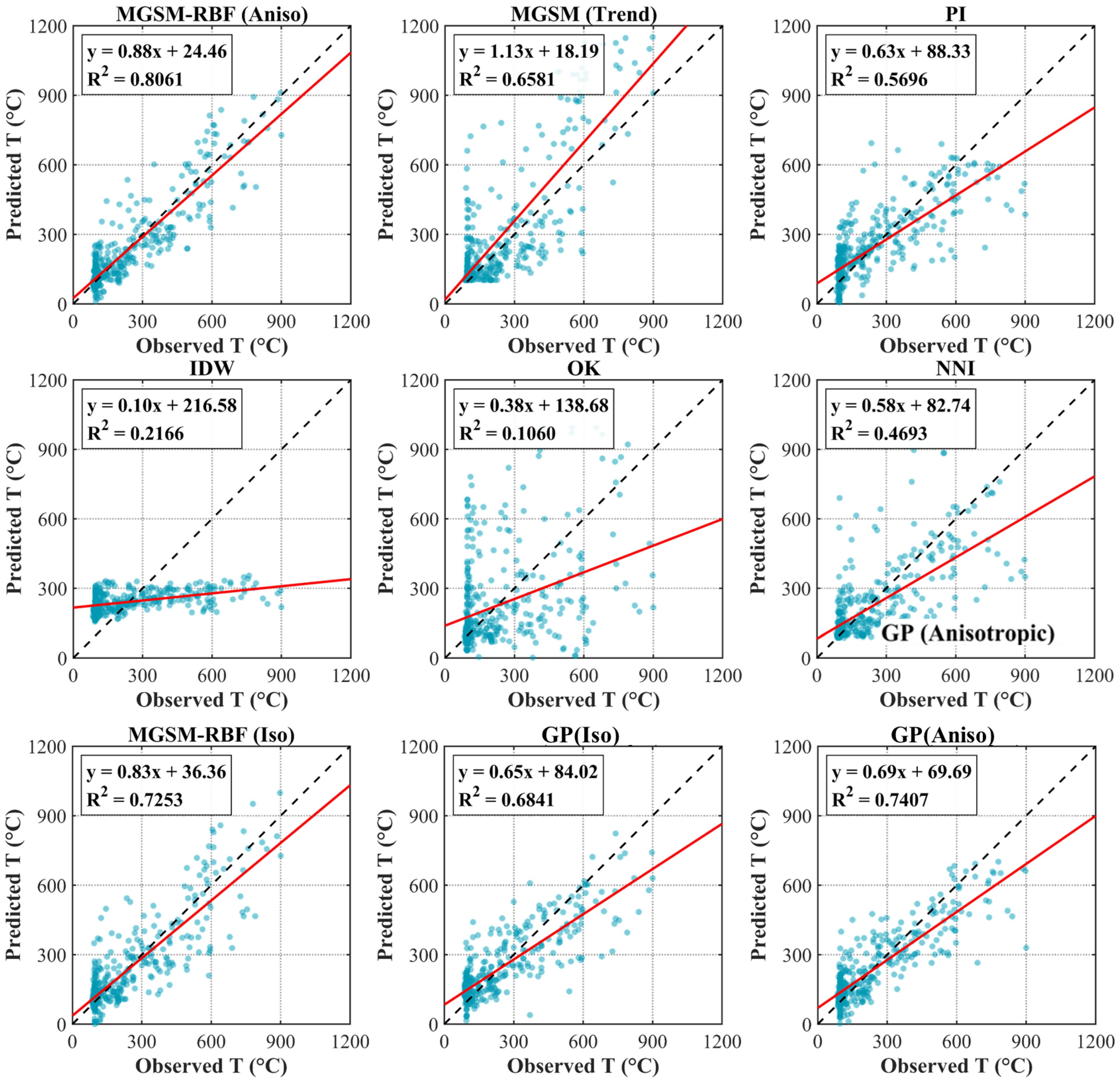
A spatially buffered cross-validation strategy was used to reduce the influence of spatial autocorrelation among neighboring borehole samples. For each validation point, samples within a horizontal radius of 15 m and a vertical distance of 25 m were excluded from the training set. These distances were selected according to the inverted diffusion scales of the identified fire sources in Table 2, with the aim of removing the most strongly correlated neighboring samples while retaining sufficient training constraints within the borehole-controlled active combustion zone. Model performance was quantified using root-mean-square error (RMSE), mean absolute error (MAE) and the coefficient of determination $R^2$. The results are shown in Figure 15 and

Table 3. Comparison of prediction accuracy metrics for different methods.

Method	RMSE ($°$C)	MAE ($°$C)	${\mathit{R}}^2$
MGSM–RBF(Aniso)	92.49	61.26	0.81
MGSM	167.10	108.76	0.66
PI	127.40	92.22	0.57
IDW	176.92	137.50	0.22
OK	245.63	172.35	0.11
NNI	145.18	88.52	0.47
MGSM–RBF (Iso)	103.79	72.07	0.72
GP (Aniso)	98.85	69.97	0.74
GP (Iso)	108.54	77.32	0.68

.

The results show that the MGSM–RBF model achieved the best overall performance among the nine methods, with an RMSE of $92.49$ $°\mathrm{C}$, an MAE of $61.26$ $°\mathrm{C}$, and an $R^2$ of 0.81. Compared with the MGSM trend model, the RMSE was reduced by 44.65%, indicating that RBF residual correction substantially improved the representation of local temperature variations. Compared with the best conventional interpolation method, PI, the RMSE was reduced by 27.40%. The MGSM-RBF model also outperformed both GP-Aniso and GP-Iso, yielding RMSE reductions of 6.43% and 14.79%, respectively.

The comparison also demonstrates the contribution of anisotropic residual correction. The isotropic MGSM–RBF model produced an RMSE of $103.79$ $°\mathrm{C}$ and an $R^2$ of 0.72, indicating lower accuracy than the anisotropic MGSM–RBF model. This improvement suggests that direction-dependent residual correction is important for representing the heterogeneous subsurface temperature field. GP-Aniso outperformed GP-Iso, further showing that anisotropy affects spatial temperature prediction. Nevertheless, the proposed MGSM–RBF model achieved higher reconstruction accuracy than both GP models, demonstrating its advantage in characterizing the complex multi-source thermal structure in the study area.

The differences in predictive performance mainly reflect the ability of each method to represent the strong heterogeneity and multi-source structure of the subsurface temperature field. The borehole data are vertically dense but horizontally sparse, and the temperature field is highly non-stationary with localized high-temperature anomalies. Conventional interpolation methods have limited capacity to capture both global thermal trends and local variations, while GP models, although flexible, do not explicitly characterize the underlying fire-source structure. The better performance of anisotropic models further indicates the importance of direction-dependent heat transfer characteristics. Overall, the proposed MGSM–RBF model achieves higher reconstruction accuracy by integrating a multi-source thermal structure model with anisotropic residual correction.

5.3. Model Assumptions and Applicability

To reconstruct the subsurface temperature field, a quasi-steady approximation and an equivalent anisotropic diffusion model were adopted. The quasi-steady approximation does not imply that coal fire combustion is strictly static. Instead, it assumes that the subsurface combustion centers and the dominant temperature-field structure remain relatively stable within the short observation period [31]. Since underground coal fires commonly persist over long periods and evolve slowly in space, inversions based on near-synchronous borehole temperature data mainly represent the spatial temperature distribution of the active combustion zone, rather than its transient evolution. Therefore, this approximation is appropriate for the objective of quasi-steady temperature-field reconstruction.

The equivalent anisotropic diffusion description was introduced to represent the dominant directional differences in subsurface heat migration. In the Sandaoba coal fire area, steeply inclined coal seams, overburden conditions, and fracture pathways may cause different heat-transfer characteristics in the vertical and horizontal directions. Therefore, the MGSM model defines separate horizontal and vertical diffusion scales. In the horizontal plane, $s_x$ and $s_y$ were combined into a unified equivalent horizontal diffusion scale $s_{xy}$. This simplification does not assume complete horizontal homogeneity. Rather, it reduces the number of inversion parameters under limited borehole constraints. If $s_x$, $s_y$, and the horizontal principal diffusion direction were all estimated independently, the model would require additional parameters and would be more prone to non-uniqueness, overfitting, and unstable fire-source localization.

To compensate for local heterogeneity not captured by the MGSM trend field, an RBF-based residual correction was introduced. The MGSM component characterizes the macroscopic temperature structure and major fire-source locations, while the RBF residual component accounts for local deviations related to fractures, material heterogeneity, and horizontal non-uniformity. Compared with purely empirical interpolation methods, MGSM–RBF not only improves temperature-field reconstruction accuracy, but also provides interpretable structural parameters, including fire-source locations, source intensities, and horizontal and vertical diffusion scales. Therefore, it provides an intermediate framework between empirical spatial interpolation and fully process-based heat-transfer simulation under limited borehole constraints.

Nevertheless, the model remains an equivalent reconstruction approach rather than a full transient heat-transfer model. The diffusion-scale parameters are inferred from borehole temperature data, rather than directly measured thermal conductivity tensors, and thermophysical or transport parameters such as thermal conductivity, heat capacity, permeability, moisture content, and fracture-controlled convection are not explicitly incorporated. These simplifications may increase uncertainty in areas affected by strong horizontal heterogeneity, pronounced directional fracture pathways, intensive ventilation, sudden collapse, rainfall infiltration, or fire-control engineering activities. In addition, UAV-derived surface thermal anomalies may be influenced by coal seam geometry, overburden conditions, fracture connectivity, and mining-induced discontinuities, and therefore should not be interpreted as direct vertical projections of underground combustion centers. In future work, numerical simulation and controlled sampling experiments should be used to systematically evaluate the effects of borehole spacing, borehole layout, and vertical sampling intervals on subsurface temperature-field reconstruction, fire-source localization, and surface–subsurface offset estimation. Additional horizontal boreholes, multi-temporal temperature monitoring, measured thermophysical properties, fracture and permeability information, and explicit anisotropic transient heat-transfer models could also be integrated to improve the process-level representation of subsurface coal fire evolution.

5.4. Sensitivity of RBF Interpolation Parameters

To evaluate the influence of RBF residual-correction parameters, a sensitivity analysis was conducted for the vertical anisotropy weight ${\lambda }_z$ and the smoothing factor c. The anisotropy weight ${\lambda }_z$ was varied from 2.0 to 10.0, and the smoothing factor c was varied from 0.2 to 1.0. As shown in

Table 4. Sensitivity of RMSE ($°$C) to anisotropy weight (${\lambda }_z$) and smoothing factor (c).

${\mathit{\lambda }}_{\mathit{z}}$	Smoothing Factor (c)
	0.2	0.4	0.6	0.8	1.0
2	117.34	115.12	116.05	115.67	118.21
4	100.15	97.42	98.18	98.05	101.33
6	96.02	95.15	92.49	95.31	98.87
8	103.25	96.88	95.62	97.45	100.12
10	113.84	111.05	109.76	117.38	123.65

, the RMSE changes continuously under different combinations of the vertical anisotropy weight ${\lambda }_z$ and smoothing factor c, without abrupt fluctuations. This indicates that the residual-correction process is generally stable over the tested parameter range.

With increasing ${\lambda }_z$, the RMSE generally first decreases and then increases. When ${\lambda }_z=2.0$, the RMSE remains relatively high for all smoothing factors, ranging from approximately 115 to $118 °\mathrm{C}$. This suggests that weak vertical anisotropic weighting is insufficient to represent the vertical variation of the subsurface temperature field. As ${\lambda }_z$ increases to 6.0, the RMSE decreases markedly and reaches its minimum value of $92.49 °\mathrm{C}$ at ${\lambda }_z=6.0$ and $c=0.6$. Further increasing ${\lambda }_z$ leads to higher RMSE values, especially when ${\lambda }_z=10.0$, indicating that excessive anisotropic weighting may weaken the ability of the residual correction to preserve local thermal anomalies.

The influence of the smoothing factor c is coupled with ${\lambda }_z$ and does not follow a simple monotonic pattern. A small c may make the residual field overly sensitive to local anomalies or measurement noise, whereas a large c may suppress local temperature variations. Therefore, a moderate smoothing level is more suitable for balancing local residual correction and spatial continuity. Considering both prediction accuracy and structural representation of the temperature field, the parameter combination ${\lambda }_z=6.0$ and $c=0.6$ lies in a relatively low-error region and provides a reasonable compromise among error control, vertical temperature-gradient representation, and residual-field spatial continuity.

5.5. UAV Thermal Infrared Observation Implications for Drilling and Coal Fire Control

The results indicate that surface thermal anomaly centers derived from UAV thermal infrared data do not correspond to simple vertical projections of subsurface fire sources, but instead represent integrated responses of heat transfer controlled by coal seam geometry and fracture pathways. In the Sandaoba coal fire area, the horizontal offsets were generally on the order of one-fifth to one-third of the burial depth, indicating an approximate and site-specific scaling relationship under steeply dipping, borehole-constrained conditions. This offset scale should not be interpreted as a universal drilling rule, but suggests that, when combined with geological constraints, UAV thermal infrared observations could provide useful reference information for interpreting subsurface fire activity.

In light of this site-specific relationship, UAV-derived thermal anomaly centers may serve as reference points for subsurface fire detection, but drilling locations should not be determined by vertical projection alone. Under similar steeply dipping and borehole-constrained geological conditions, drilling positions may be considered within a candidate search zone around the surface anomaly center, with attention to the dip-related offset direction indicated by local geological constraints. For elongated or complex anomaly patterns, increased drilling density and supplementary verification in both dip and strike directions may help reduce uncertainty. Overall, UAV thermal infrared data provide a useful site-specific quantitative reference for linking surface observations with subsurface fire source distribution, offering practical guidance for supporting drilling design and fire control strategies under comparable geological conditions.

6. Conclusions

This study reconstructs the subsurface temperature field and quantifies the spatial relationship between surface and subsurface thermal anomalies using UAV thermal infrared data and borehole measurements in the Sandaoba coal fire area, Xinjiang. A combined approach integrating surface anomaly extraction, subsurface inversion, and spatial offset analysis is established. The main conclusions are as follows:

A robust method for extracting surface thermal anomalies is developed to reduce fragmentation in UAV thermal infrared observations. A thermal anomaly threshold of 15.9 $°\mathrm{C}$, combined with adaptive kernel density estimation, generates a continuous intensity field. Based on a normalized intensity threshold of 0.25, two stable anomaly centers are identified, exhibiting compact and elongated spatial patterns. The intensity-weighted centroid provides a stable representation of surface response locations.

A spatial-structure constrained inversion method is developed to reconstruct the subsurface temperature field and characterize the spatial structure of multiple fire sources. The MGSM–RBF model identifies three distinct fire sources, with higher temperatures in the western sources (1096.93 $°\mathrm{C}$ and 847.85 $°\mathrm{C}$) and a weaker eastern source (467.71 $°\mathrm{C}$). The main combustion zone is concentrated at depths of 30–55 m. The model achieves improved accuracy compared to conventional methods, with an $R^2$ of 0.81 and an RMSE of 92.49 $°\mathrm{C}$.

A site-specific spatial offset between subsurface fire sources and surface thermal anomaly centers was observed, with horizontal distances of approximately 14.5 m, 13.4 m, and 7.5 m in the Sandaoba coal fire area. The dimensionless offset coefficient ranges from 0.19 to 0.31, suggesting that the horizontal offset is approximately one-fifth to one-third of the burial depth under the steeply dipping and borehole-constrained conditions. This non-vertical correspondence indicates that geological structures may redirect heat migration along preferential structural pathways, producing complex offset patterns. Depth-resolved analysis further shows that surface thermal responses are jointly controlled by multi-source superposition, structural pathways, and depth-dependent heat migration.

The results provide a site-specific reference for drilling and fire control design under similar geological conditions. Surface thermal anomaly centers should not be directly treated as vertical projections of subsurface fire sources. Instead, drilling design may consider candidate zones along the dip-related offset direction, with supplementary verification for complex anomalies. The offset-analysis framework could support drilling layout optimization in comparable coal fire areas.