TCF-VQGAN: Two-Stage Codebook Fusion Vector-Quantized GAN for Multimodal Remote Sensing Image Cloud Removal

Highlights

What are the main findings?

• TCF-VQ GAN achieves state-of-the-art cloud removal performance, with better MAE, SAM, PSNR, and SSIM than existing multimodal fusion and GAN-based methods.
• The two-stage training strategy uses unpaired multimodal data for codebook pre-training and then improves results through fusion fine-tuning with limited paired samples.

What are the implications of the main findings?

• Additional unpaired multimodal data serve as an effective pretraining source for learning transferable priors, which can boost cloud removal performance under limited paired supervision.
• The SCGC module and DW²A loss offer a practical design for multimodal remote sensing reconstruction, especially under irregular cloud occlusion.

Abstract

With the advancement of remote sensing technology, image acquisition has become more convenient and the amount of information captured has significantly increased, playing a vital role in numerous fields. However, cloud cover often results in missing image data, severely affecting data usability. In recent years, although deep learning methods have made progress in cloud removal tasks, the complexity of modeling multispectral band relationships and the scarcity of paired data remain major challenges. To address this, this paper proposes a two-stage codebook fusion vector-quantized generative adversarial network (TCF-VQ GAN) and a training framework. The first stage employs synthetic aperture radar (SAR), MODIS, and cloud-free data for unsupervised training; the second stage performs fusion fine-tuning using SAR and MODIS on paired cloudy/cloud-free data. The model incorporates a space-channel jointed gated convolution (SCGC) module to model irregular cloud cover and combines channel attention for band selection, while a dynamically weighted wavelet alignment loss function (DW²A) is designed to enhance multiscale feature representation. Experiments on the SEN12MS-CR and SMILE-CR datasets demonstrate that the proposed method outperforms existing methods across all metrics: on SEN12MS-CR, PSNR is 31.0397 and SAM is 4.7243; they are 33.5191 and 2.1663, respectively, on SMILE-CR. Furthermore, under fixed paired data conditions, simply adding auxiliary and cloud-free data further improves performance, validating the method’s effectiveness in data-scarce scenarios.

1. Introduction

In recent years, with the development of multispectral remote sensing equipment and high-resolution imaging technology, remote sensing capabilities have significantly improved. Modern remote sensing equipment can acquire rich ground-level information under varying conditions of time, weather, and angle; in particular, optical remote sensing and SAR have enabled all-weather, multimodal data collection. Among the various types of remote sensing data, medium-resolution multispectral imagery is widely used in land cover classification, crop growth analysis, urban building identification, and forest surveys due to its intuitive and easy-to-interpret nature. However, such images are susceptible to cloud interference. According to long-term observations by the International Satellite Cloud-Climate Project (ISCCP), approximately 67% of surface remote sensing images are affected by clouds to varying degrees [1], which impacts the utilization of satellite resources and interferes with time-sensitive applications, such as natural disaster response or crop yield forecasting. Remote sensing image cloud removal aims to recover original ground object information from cloud-obscured images, making it a topic of significant research importance in the current context.

With the advancement of deep learning, remote sensing cloud removal has gradually shifted from early traditional statistical methods to data-driven deep learning approaches. Traditional methods include interpolation [2], pixel replacement, and dictionary learning [3,4,5]. Deep learning methods are generally categorized into two types: image reconstruction and information fusion. Image reconstruction focuses on restoring partially degraded images; for example, thin clouds typically do not completely obscure ground object information, and satisfactory reconstruction quality can often be achieved using only optical bands. However, restoration becomes challenging when thick clouds or complex ground features are present [6]. Information fusion compensates for the limitations of single-source data by integrating data from different sensors, time periods, or scales; such methods are commonly employed for thick cloud removal [7]. For instance, incorporating SAR data can provide structural and textural information missing from optical imagery, thereby enhancing cloud removal performance [8]. However, due to significant differences in imaging mechanisms and features between SAR and optical imagery, efficient modal fusion remains a key challenge. Although deep learning methods demonstrate excellent performance in terms of results, they typically rely on supervised training, whereas the core bottleneck in cloud removal tasks lies in the lack of strictly corresponding pairs of cloud-covered and cloud-free images. Existing datasets are primarily constructed in two ways: one uses image pairs acquired at different times over the same area, which is realistic but complex to process [9,10]; the other generates clouds through noise sampling and cloud simulation to ensure consistency between input and labels, but this approach struggles to closely mimic real-world conditions, leading to limited performance in practical applications [11].

To address the aforementioned issues, this paper conducts research based on the Vector Quantized Generative Adversarial Network (VQ-GAN). VQ-GAN builds upon the Vector Quantized Variational Autoencoder (VQ-VAE) by replacing continuous latent space variables with discrete codebooks and integrating them into the GAN training framework, where the encoder maps the input to the closest codebook entry before reconstruction [12,13,14]. Inspired by this, this paper proposes the TCF-VQ GAN and a two-stage training framework based on this model, dividing the cloud removal task into a codebook learning stage and a fusion fine-tuning stage. Within this framework, a spatial-channel jointed gated convolution (SCGC) module is designed to achieve efficient feature fusion between multispectral and SAR/MODIS data; simultaneously, to address the multi-scale reconstruction problem in multi-channel remote sensing imagery, we introduce the dynamically weighted wavelet alignment loss (DW²A Loss) to enhance the model’s perceptual consistency and reconstruction accuracy. The main contributions of this paper are detailed as follows:

1.

To address the reliance on large-scale cloudy/cloud-free paired data and the limitations in reconstruction fidelity found in deep learning-based cloud removal methods, this paper proposes a two-stage training strategy and the VQ-GAN model employed under this strategy. The model first undergoes codebook pre-training on SAR/MODIS and cloud-free data, followed by fusion fine-tuning using a small amount of cloudy/cloud-free paired data. Experiments demonstrate that simply expanding the dataset size in Stage I improves model performance and reduces the number of optimization steps required in Stage II.

2.

To address the issue that cloud occlusion in input images weakens the assumption of local invariance in convolutions, we designed a spatial-channel jointed gated convolution (SCGC) module. By employing gated convolutions and channel attention mechanisms, this module models irregular cloud patterns and enhances multispectral feature representation capabilities. Forward feature visualization results indicate that the gating weights can explicitly model cloud regions, enabling selective extraction of structural information.

3.

To address the limitations of traditional multi-scale perceptual losses—which exhibit limited perceptual capabilities on multispectral remote sensing images and rely on pre-trained models—this paper proposes DW²A Loss. By dynamically weighting and aligning image details across different scales, it improves reconstruction quality and perceptual consistency.

The paper is organized as follows: Section 2 describes related work, including the definition of the cloud removal task, an introduction to VQ-GAN, and existing research on VQ-GAN in visual tasks and cloud removal. Section 3 details the proposed model architecture, training framework, and loss function design. Section 4 presents experimental results and ablation studies on key design elements. Section 5 discusses the impact of training with data from different modal combinations on performance metrics, the distinct characteristics of codebook representations across the two stages and the limitations of cloud and shadow masks in the loss function. Finally, Section 6 concludes the paper.

2. Related Work

In this section, we first review existing cloud removal methods based on adversarial learning and multimodal fusion, followed by an overview of the research background of VQ-GAN. Finally, we present existing research on VQ-GAN in the field of cloud removal and other visual tasks.

2.1. Cloud Removal Methods Based on Adversarial Learning and Multimodal Fusion

In deep learning approaches, the task of remote sensing cloud removal can be divided into image reconstruction and multimodal information fusion. GANs have become a commonly used research framework due to their powerful ability to model complex distributions. The generator produces realistic images through adversarial training, while the discriminator enhances its ability to distinguish between real and generated data, thereby achieving high-fidelity reconstruction [15,16,17]. Building on this foundation, researchers have gradually integrated GANs with multimodal information fusion. Within the GAN framework, Pan et al. designed a multi-directional spatial attention generator to perform cloud removal in the RGB bands [18]; following the introduction of conditional generative adversarial networks (cGANs), Enomoto et al. combined multispectral and near-infrared information to achieve partial cloud-penetrating reconstruction [19]; regarding cross-modal mapping, Bermudez et al. utilized a GAN model to convert SAR data into multispectral images [20].

However, when using a single modality as input, it is often difficult to address issues such as thick clouds or the absence of high-frequency textures. Therefore, many studies have introduced additional data, such as SAR, as a condition for cloud removal. Still within the GAN framework, Gao et al. proposed first mapping SAR to a cloud-free image, then combining it with a cloud-containing image for secondary reconstruction, and training using a modal fusion loss [21]. Among non-GAN methods, Meraner et al. proposed simultaneously inputting SAR and multispectral images for joint reconstruction via a dense residual network [22]; Xu et al. employed a global fusion module to achieve multimodal feature fusion [23]; Li et al. proposed a hierarchical spectral and structural preservation fusion network, which improved reconstruction performance in areas with medium-to-thick clouds and shadows through channel attention and a collaborative optimization loss [24]. Gu et al. proposed a heterogeneous parallel network, designing dual branches to process conditioned and contaminated images separately, followed by decoding through a heterogeneous feature fusion block [25].

At the framework level, GAN-based methods often suffer from instability inherent to GANs; an improper balance between pixel reconstruction loss and adversarial loss can easily lead to insufficient fidelity in the generated results. In recent years, diffusion models have been introduced into remote sensing cloud removal tasks due to their stable training and strong distribution modeling capabilities, outperforming GANs in terms of detail recovery and structural consistency. Jing et al. proposed DDPM-CR, which extracts multiscale diffusion features by fusing cloud-covered optical and SAR data, and combines an attention-based cloud removal head with a cloud-region-specific loss function to achieve high-fidelity reconstruction under both thin and thick cloud conditions [26]. Zou et al. proposed DiffCR, which decouples the conditional encoder from the time-conditional fusion module to perform multi-scale feature fusion. By adopting a prediction strategy that directly regresses to the cloud-free image, the method achieves few-step sampling-based cloud removal with low parameters and computational complexity [27]. Liu et al. proposed EMRDM, which establishes a mapping between cloud-covered and cloud-free images by improving the stochastic differential equation of the diffusion process and reverse modeling of ODEs. They introduced a preconditioned denoiser and deterministic/stochastic sampling strategies and extended the method to multi-temporal sequence modeling to enhance temporal consistency and reconstruction performance [28].

At the data level, a common issue among most methods is that effective training heavily relies on large-scale paired data, yet obtaining high-quality paired samples in remote sensing scenarios remains challenging. Regarding network architecture design, methods using dual-branch networks combined with fusion modules are often constrained by the performance of the fusion modules themselves when modeling relationships between multimodal data, and the use of deep separable convolutions to reduce the number of parameters tends to exacerbate this problem.

2.2. VQ-GAN

VQ-GAN is derived from integrating VQ-VAE into the GAN framework. Before introducing VQ-VAE, it is helpful to review the concept of dictionary learning to better understand sparse image representation. Dictionary learning was widely used in early cloud-removal tasks, where an “overcomplete dictionary”—a set of representative image features—was learned from a large number of cloud-free images and then used to reconstruct the images in the regions obscured by clouds. Its core idea is to leverage the sparsity of images by representing them as linear combinations of a few atoms in a dictionary [3,4,5]. VQ-VAE replaces the latent space in VAE—which adheres to specific distribution assumptions—with a discrete codebook. Instead of using reparameterization, it replaces the encoder’s output with a codebook vector via minimum-distance lookup and then the decoder generates the output [14]. This approach allows for flexible configuration of the latent space size, eliminates assumptions about the latent space distribution, enhances the expressive power of the codebook, and effectively mitigates the posterior collapse problem [13]. However, codebook lookup is non-differentiable during backpropagation. There are two primary methods for updating the codebook: the first is the Straight-Through Estimator (STE), which copies the gradient of the encoder’s output onto the codebook vectors, allowing them to be updated via backpropagation [29]. Defining the encoder’s output as ${\mathcal{Z}}_e$, the codebook entries as ${\mathcal{C}}_k$, and the quantization result as ${\mathcal{Z}}_q$, where sg[·] is the truncated gradient, the mathematical expression for the gradient-through estimator is shown in Equation (1).

$${\mathcal{Z}}_q={\mathcal{Z}}_e+sg\left[{\mathcal{C}}_k-{\mathcal{Z}}_e\right]$$

(1)

Another method for updating the codebook involves using exponential moving averages (EMAs). When updating the codebook with the EMA of the encoder’s output, this approach is more stable than STE when the distribution varies significantly [13]. Let $\gamma$ denote the decay factor; the codebook updated via the EMA at time t is given by Equation (2).

$${\mathcal{Z}}_q^t=\gamma {\mathcal{Z}}_q^{t-1}+(1-\gamma ){\mathcal{Z}}_e^t$$

(2)

VQ-GAN combines the complex distribution modeling capabilities of GANs with the flexible latent space modeling capabilities of VQ-VAE. By introducing an adversarial loss, VQ-GAN is capable of generating more realistic and detailed images. Compared to continuous latent variables, discrete codebooks not only offer greater expressive power but also, when using Transformer-based models in computer vision, provide codebook vectors with larger receptive fields and richer high-dimensional semantic information than methods that segment images into patches and convert them into vectors.

2.3. Applications of VQ-GAN in Visual Tasks

Since its introduction, VQ-GAN has been widely applied to various computer vision tasks. Esser et al. initially applied VQ-GAN to high-resolution image generation, converting image structures into codebook vectors through unsupervised training within the GAN framework and combining this with a Transformer for image generation [14]. In the field of image denoising, although the models proposed by Xia and Jia, as well as those by Ling and Zhang, are not VQ-GANs, their sparse representation methods based on dictionary learning have provided valuable insights for understanding image feature reconstruction [30,31]. In the field of image restoration, Wang et al. introduced an attention mechanism into VQ-GAN and designed a two-stage training strategy: first performing unsupervised codebook learning on undamaged images and then fine-tuning the model using damaged images. This approach achieved significant results in face image restoration tasks, and the model design and training framework in this paper were also inspired by this work [32,33]. In remote sensing image processing, codebooks are also commonly used for latent space representations in diffusion models. Liu et al. proposed a VQ-GAN method that maps hyperspectral data to a low-dimensional latent space before diffusion, effectively addressing the problem of high-dimensional noise prediction [34]; Wang et al. proposed a two-stage model for thin cloud removal involving coarse-to-fine restoration, achieving high-quality cloud removal through Pixel-CR and a pre-trained VQ-VAE encoder [35]. The aforementioned studies demonstrate that VQ-GAN and its discrete representation approach hold significant potential in image reconstruction and generation. However, their application in remote sensing image cloud removal remains limited, with most studies focusing on dimensionality reduction in the latent space of diffusion models, failing to fully leverage the information storage and representation capabilities of codebooks. To address this, this paper proposes a two-stage cloud removal framework that combines unsupervised and supervised learning and fully exploits the potential of VQ-GAN through specific architectural design.

3. Methodology

3.1. Problem Definition

This paper defines the cloud removal task as a two-stage composite task comprising information representation and optimized reconstruction. To ensure high fidelity of surface information during the cloud-removal reconstruction process, the network should first be able to explicitly learn surface feature information and then fine-tune it using paired data. Given a registered cloud-free image and a set of auxiliary images (SAR, MODIS, or both) ${\mathcal{D}}_{clean}=\{I_{aux}^{\left\{i\right\}},I_{gt}^{\left\{i\right\}}\}$, the encoder and decoder are denoted as Enc(·) and Dec(·), respectively. The quantization process of codebook matching is defined as quant(·) and the loss function is $\mathcal{L}$. The training process for Stage I can then be expressed as Equation (3):

$$\begin{array}{cc}\hfill \underset{Enc,Dec,C}{min}& {\mathbb{E}}_{(I_{\mathrm{aux}},I_{\mathrm{gt}})\sim {\mathcal{D}}_{\mathrm{clean}}}\left[\mathcal{L}\left(I_{\mathrm{gt}},Dec\left(quant(Enc(I_{\mathrm{gt}},I_{\mathrm{aux}}))\right)\right)\right]\hfill \\ \hfill \mathrm{s}.\mathrm{t}.& quant\left(z\right)=arg\underset{c_k\in \mathcal{C}}{min}{\parallel z_e-c_k\parallel }_2^2,\hfill \end{array}$$

(3)

where $\mathcal{C}={\{{\mathrm{c}}_k\in {\mathbb{R}}^d\}}_{k=1}^n$ denotes a predefined codebook. Upon completion of Stage I training, the model weights are saved. In Stage II, only the input data needs to be replaced, and the model is initialized using the weights from Stage I, enabling it to possess a certain level of feature representation capability from the outset of Stage II. Given a registered dataset consisting of cloud-covered images, cloud-free images, and auxiliary images ${\mathcal{D}}_{pair}=\{I_{cloudy}^{\left\{i\right\}},I_{aux}^{\left\{i\right\}},I_{gt}^{\left\{i\right\}}\}$, the training process for Stage II can be expressed as Equation (4):

$$\begin{array}{cc}\hfill \underset{Enc,Dec}{min}& {\mathbb{E}}_{(I_{\mathrm{cloudy}},I_{\mathrm{aux}},I_{\mathrm{gt}})\sim {\mathcal{D}}_{\mathrm{pair}}}\left[\mathcal{L}\left(I_{\mathrm{gt}},Dec\left(quant(Enc(I_{\mathrm{cloudy}},I_{\mathrm{aux}}))\right)\right)\right]\hfill \\ \hfill \mathrm{s}.\mathrm{t}.& quant\left(z\right)=arg\underset{c_k\in \mathcal{C}}{min}{\parallel z_e-c_k\parallel }_2^2\hfill \end{array}$$

(4)

Using the approach described above, this paper breaks down the complex task of cloud removal into two relatively independent yet closely related subtasks: codebook learning and fusion fine-tuning. During the codebook learning phase, the model utilizes registered cloud-free images and auxiliary data to extract abstract representations of surface features and perform multimodal information fusion. Subsequently, in the fusion fine-tuning phase, by leveraging the prior knowledge acquired in Stage I, the model is able to generate more realistic and high-fidelity texture details.

3.2. Training Framework

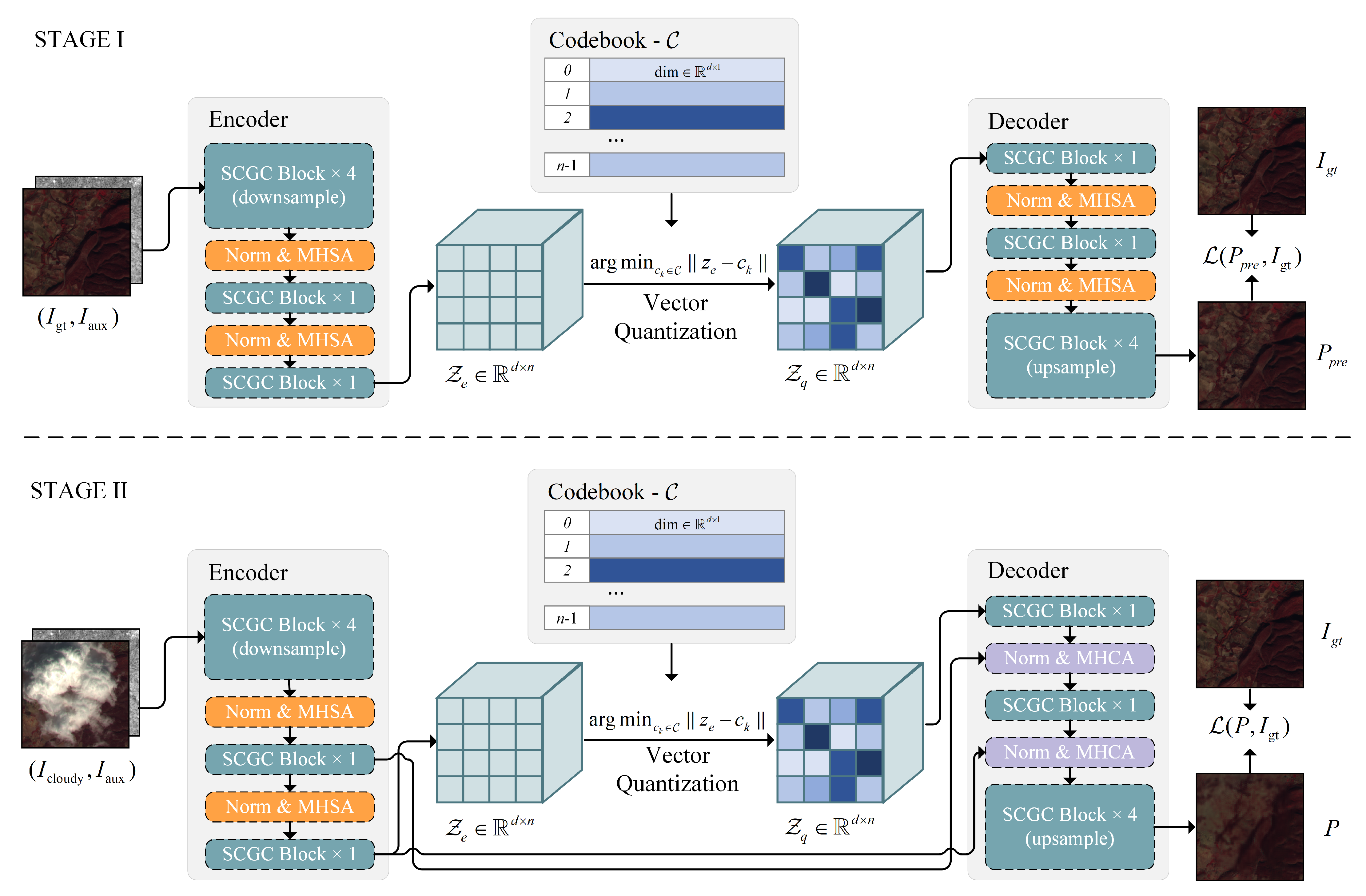
Building on the problem formulation described earlier, this paper designs the TCF-VQ GAN network architecture within the proposed two-stage training framework. The overall architecture is shown in Figure 1.

From the perspective of the training framework, network training is divided into two phases. The primary objective of Stage I is to compress the feature information of cloud-free images and store it in a codebook through unsupervised learning. Concurrently, auxiliary image data is incorporated during this phase to enable the model to perform fusion learning between multispectral and SAR images. Specifically, the model first receives cloud-free images and auxiliary images, generates unquantized vectors via the encoder, then matches the vector with the codebook vector with the smallest distance and replaces it with that codebook vector, and finally uses the decoder to decode the quantized vectors and produce the output. In this paper, the codebook is updated using the EMA method.

Upon completion of Stage I training, the encoder is already capable of fusing multimodal data and generating high-quality codebook vectors corresponding to the codebook. Although the model already possesses a certain degree of cloud removal capability under low-cloud conditions, it currently cannot process images containing clouds. Therefore, Stage II training is required. Compared to Stage I, the network architecture remains unchanged in Stage II training, but the self-attention computation in the decoder is replaced with cross-attention computation. This phase employs supervised training, with cloud-containing images and SAR images as inputs and cloud-free images as outputs. In cross-attention, the query is composed of quantized vectors, while the key and value are derived from the encoder’s pre-quantization features. This design leverages the modeling capabilities of cross-attention while avoiding the posterior collapse problem [36]. Through fine-tuning in Stage II, the model is enabled to gradually learn how to extract features and perform reconstruction from inputs with varying degrees of cloud contamination, while leveraging prior knowledge of clean ground objects.

3.3. Model Architecture

From an overall architectural perspective, the encoder and decoder primarily consist of alternating convolutional modules (SCGC Blocks) and attention layers used for feature extraction of codebook entries. Taking an input image with spatial dimensions of ${256}^2$ as an example, the network adopts an encoder-decoder architecture. Both the encoder and decoder consist of alternating stacks of SCGC blocks and attention layers designed to learn features of codebook entries, thereby simultaneously modeling local textures and global dependencies. During the encoding phase, the input first passes through four SCGC Blocks for preliminary feature extraction, enhancing representational capacity while maintaining a spatial resolution of ${256}^2$. Subsequently, through three rounds of downsampling, the resolution is progressively reduced to ${128}^2$, ${64}^2$, and, finally, ${32}^2$ at the bottleneck layer, with the channel dimension correspondingly increased to enhance semantic expression. At the ${32}^2$ -level, the features are flattened into a sequence and fed into an attention module for global modeling and then restored to a spatial structure and further processed through SCGC blocks for feature extraction. This alternating SCGC—Attention—SCGC process is repeated twice at the bottleneck to strengthen multiscale information interaction. During the quantization stage, vector quantization is employed to map continuous features to a codebook space to obtain discrete representations and features are restored in stages during the decoding process. In Stage I, after the quantized vectors are restored to ${32}^2$ features, two rounds of attention computation + SCGC Block are repeated to enhance reconstruction expressiveness. In Stage II, a cross-attention mechanism is additionally introduced to align and fuse the pre-quantization continuous features with the post-quantization discrete representations, thereby improving information compensation and consistency constraints. Finally, the decoder gradually restores the resolution to ${256}^2$ through four SCGC blocks combined with three rounds of upsampling and computes a reconstruction loss at the output to ensure consistency between the generated results and the true cloud-free imagery. Additionally, the specific implementation details and code for this method are described in the open-source repository provided at the end of the paper.

3.3.1. SCGC Block

Compared to other image reconstruction tasks, such as image defogging, a distinctive feature of the cloud removal task is that the spatial distribution of cloud coverage is highly non-uniform. The degree of cloud coverage varies significantly across different regions; some areas are almost cloud-free, while others are completely obscured by thick clouds. These spatial variations significantly weaken the translation-invariant inductive bias on which convolutional neural networks rely. Furthermore, in the context of this specific task, cloud removal from multispectral remote sensing images is more complex than reconstruction tasks relying solely on the three RGB channels, as there are more intricate inter-channel relationships.

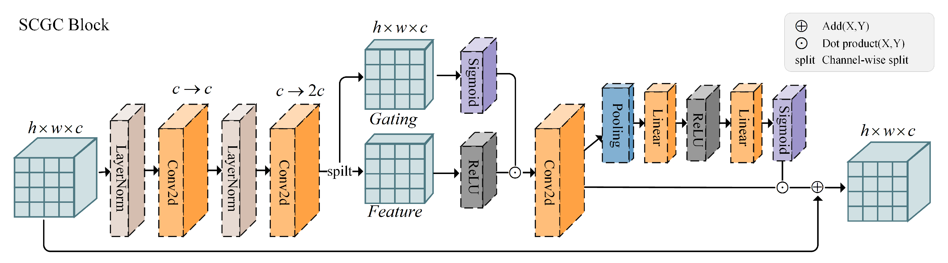
To address these issues, a joint feature extraction module combining gated convolutions and channel attention was designed to enhance feature representation capabilities. The overall module design is shown in Figure 2.

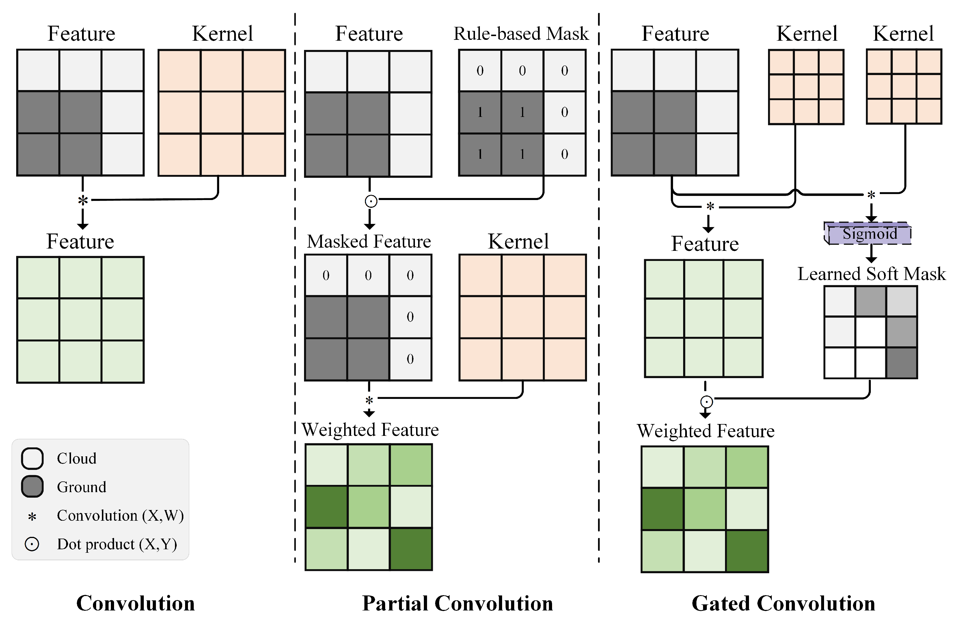
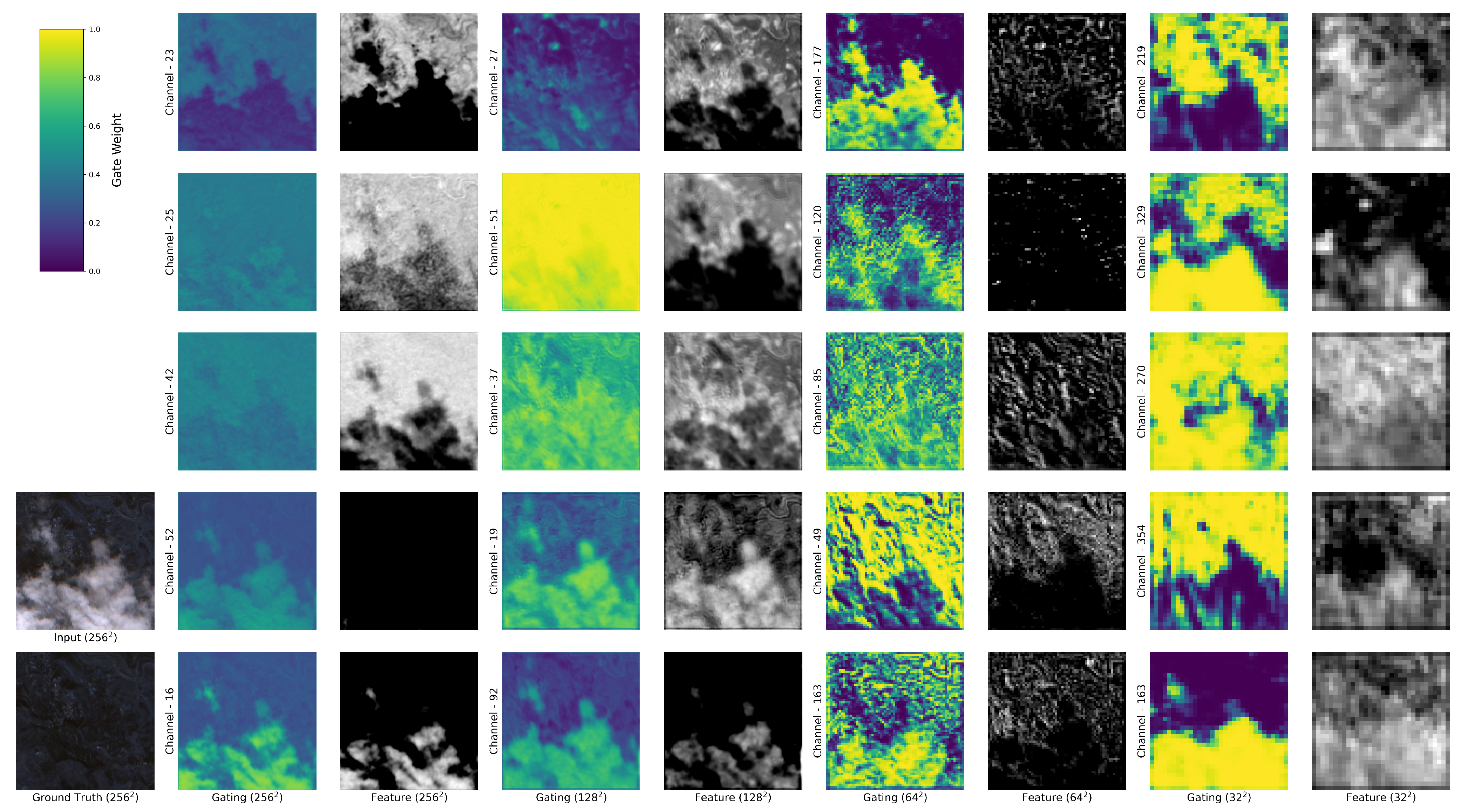
First, to address the issue of significant variations in degradation levels across different regions, a gated convolutional operator was introduced. Gated convolution is a further refinement of partial convolution [37]. Unlike partial convolution, which relies on rule-based masks and cannot adaptively learn, gated convolution divides features into a gating component and a feature component, which are then fused via a Hadamard product. This enables it to adaptively detect valid pixels within irregular regions, as shown in Equation (5) [38]. Here, ∗ denotes the convolution operation. The convolution kernels ${\mathcal{W}}_g$ and ${\mathcal{W}}_f$ act on different branches, respectively. The sigmoid function $\sigma$ maps the gating values to [0, 1] to serve as gating weights, while the activation function $\varphi$ can be freely selected. Figure 3 provides a more intuitive representation of the computational processes for standard convolution, partial convolution, and gated convolution, respectively. In the ablation experiments, the features of randomly sampled channels during the forward pass at different downsampling levels after model training were analyzed. The gating values after passing through the sigmoid function serve as weights, while “Feature” denotes the feature itself. It can be observed that this mechanism enables the convolution operation to perceive cloud layers across different spatial dimensions, thereby dynamically suppressing or enhancing features.

$$\begin{array}{cc}\hfill Gatin{g}_{y,x}& ={\mathcal{W}}_g\begin{array}{c}\hfill \ast \end{array}I\hfill \\ \hfill Featur{e}_{y,x}& ={\mathcal{W}}_f\begin{array}{c}\hfill \ast \end{array}I\hfill \\ \hfill O_{y,x}=\varphi (Featur{e}_{y,x}& )\odot \sigma \left(Gatin{g}_{y,x}\right)\hfill \end{array}$$

(5)

Then, to address the complex relationships among channels in multispectral images, this paper introduces a channel attention mechanism. The channel attention mechanism aims to adaptively model the relationships between different channels and highlight key information by assigning weights to each channel of the feature map. Compared to tasks that use only RGB or RGBA images, channel attention enables more effective feature extraction in multispectral remote sensing images. The Squeeze-Excitation (SE) attention mechanism is an early channel attention method. It compresses each channel into a scalar vector via global average pooling, then applies a nonlinear transformation through a multi-layer perceptron to learn channel weights, and, finally, weights the original channel features [39]. Building upon the SE mechanism, numerous studies have proposed various variants. For instance, Qin et al. modeled channel attention as a compression problem, utilizing the Discrete Cosine Transform (DCT) to achieve frequency-domain channel weighting [40]. Our experiments reveal that despite its relative simplicity, the SE mechanism performs better in multispectral image scenarios; its specific performance will be demonstrated in ablation experiments.

Unlike methods such as HPN-CR that use multi-branch structures to fuse modal data, this paper achieves dynamic fusion of different modal data throughout the entire network through the design of the SCGC module, which constitutes the core of the network. Taking SAR and multispectral images as inputs, they are represented as $I_{sar}$ and $I_{ms}$, respectively. The SCGC module first concatenates them along the channel dimension and performs gated convolutions with a Pre-Norm structure.

$$\begin{array}{cc}\hfill I_{in}& =Concat(I_{sar},I_{ms}),\hfill \\ \hfill h_{sar\_ms}& =GatedConv\left(LayerNorm\left(Conv\left(I_{in}\right)\right)\right)\hfill \end{array}$$

(6)

This step first suppresses and enhances information across modalities in the spatial dimension. For multispectral images, it effectively detects cloud regions, as shown in ablation studies. For SAR images, spatial information suppression effectively reduces speckle noise that occurs during the imaging process [23]. After suppressing features in the spatial dimension, the information in the channel dimension still needs to be fused. SCGC automatically weights the relative importance of information across channels via a channel attention mechanism, as shown in Equation (7).

$$\begin{array}{cc}\hfill h_{channel}& =AvgPoo{l}_{2D}\left(h_{sar\_ms}\right),\hfill \\ \hfill w_{fuse}& =\sigma \left(MLP\left(h_{channel}\right)\right),\hfill \\ \hfill h_{fused}& =h_{sar\_ms}\odot w_{fuse}\hfill \end{array}$$

(7)

First, global average pooling is applied to the features computed by spatial attention to obtain their channel-level representations $h_{channel}$. These are then transformed via an MLP, followed by a Sigmoid function to convert them into weight features within the range $[0,1]$. These weight features represent the relative importance of different channels, i.e., the relative importance of weights across different modalities. Finally, multiplying them by the initial features yields the modality-fused features $h_{fused}$. The method proposed in this paper avoids the design of multi-branch network architectures through its modular design, thereby improving its generalization and efficiency in multi-modal data fusion without the need to design new conditional fusion heads. Experiments demonstrate that without modifying the model structure, the network performs excellently on both dual-modal (SAR + multispectral) and triple-modal (SAR + MODIS + multispectral) inputs.

3.3.2. Self-Attention and Cross-Attention

In recent years, with the widespread adoption of Transformer models, dot-product attention mechanisms have been extensively incorporated into various networks [41,42,43]. This mechanism does not rely on inductive biases, can directly model intrinsic relationships from the data, and possesses the ability to model long-range dependencies [44]. Its computational form is shown in Equation (8), where the query (Q), key (K), and value (V) are obtained through linear transformations and the attention matrix is denoted as A:

$$Attention(Q,K,V)=Softmax({\displaystyle \frac{Q{K}^{\top }}{\sqrt{d}}})V$$

(8)

In Stage I, after downsampling the image to ${32}^2$, a self-attention module is introduced following the final downsampling step to expand the receptive field of the codebook vectors. The features are flattened and sequentially passed through the self-attention and SCGC blocks; this process is repeated once before quantization. The decoder adopts a “convolution-self-attention” structure that is symmetric to the encoder, thereby enhancing the codebook’s ability to model global semantics. In Stage II, the decoder’s self-attention is replaced with cross-attention, where the queries come from the quantized vectors and the keys and values originate from the convolutional features following the encoder’s self-attention. This design enables the quantized object features to integrate complementary information from the features prior to quantization during the decoding stage, thereby obtaining richer representations.

$$\begin{array}{cc}\hfill Attention& (z,h_k,h_v)=\sum _i{a}_i{h}_{v,i}=\left[h\right|z]\hfill \\ \hfill & a_i={\displaystyle \frac{exp(z^{\top }{h}_{k,i})}{{\sum }_{i}exp(z^{\top }{h}_{k,i})}}\hfill \end{array}$$

(9)

From a probabilistic perspective, the attention mechanism can be viewed as a conditional probability [45]; that is, cross-attention can be expressed in terms of conditional expectation, as shown in Equation (9), where ${\sum }_i{\alpha }_i=1$ and ${\alpha }_i\ge 0$. Therefore, this method can be understood as modeling the expected features extracted by the encoder from the cloud-containing image in Stage II, conditional on the object features learned in Stage I.

3.4. Loss Function

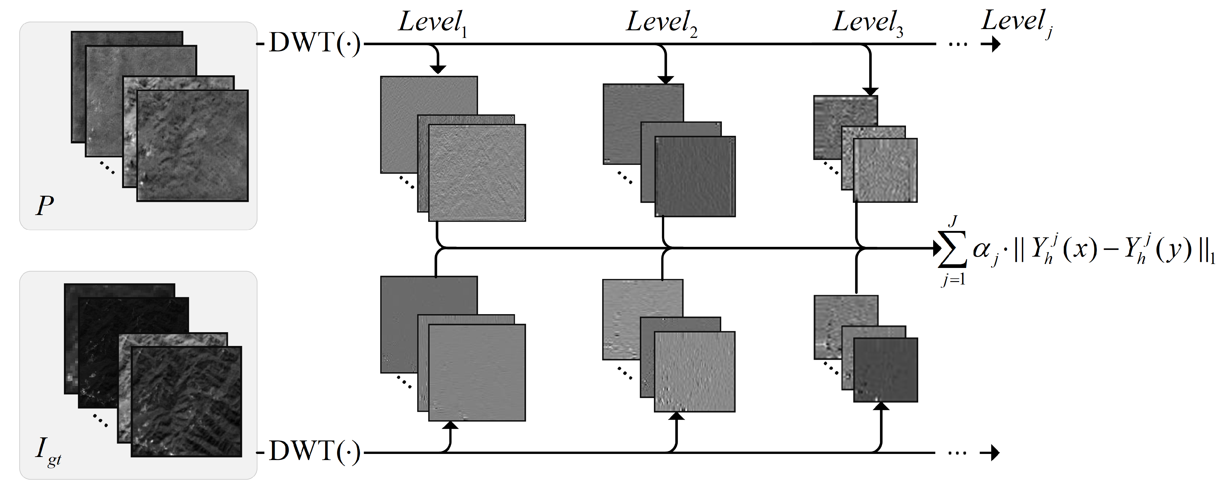
In addition to improving the fidelity of the results, visual quality is also a key evaluation metric. Traditional methods often employ multi-scale perceptual loss based on pre-trained VGG networks to enhance the texture and structural consistency of generated images [46]. However, this loss relies on VGG models that are only applicable to RGB images and lack adaptability to other bands in multispectral data. To address this, this paper proposes a Dynamically Weighted Wavelet Alignment Loss (DW²A Loss) based on the Discrete Wavelet Transform (DWT) [47]. This method utilizes DWT to decompose the generated image and the target image into multi-scale high-frequency subbands, achieving alignment of texture and edge details by calculating the $L1$ difference of high-frequency components ($LH$, $HL$, $HH$) at each scale. DW²A Loss introduces learnable dynamic weights, which adaptively adjust the importance of each scale after Softmax normalization.

Its form is shown in Equation (10), which includes two adjustable hyperparameters: the decomposition level j and the wavelet basis functions. Let $\mathcal{W}={\{w_j\in \mathbb{R}\}}_{j=1}^J$ denote the learnable weights, ${\alpha }_j$ be the weights after Softmax normalization, and $Y_h^j\left(x\right)$ be the high-frequency components ($LH$, $HL$, $HH$) at the jth decomposition level. The calculation of the loss function is shown in Equation (10) and the specific structure is illustrated in Figure 4.

$$\begin{array}{cc}\hfill DWT\left(x\right)& =\{Y_h^1\left(x\right),Y_h^2\left(x\right),...,Y_h^J\left(x\right)\}\hfill \\ \hfill {\mathcal{L}}_{D{W}^{2}A}(x,y)& ={\displaystyle \sum _{j=1}^J}{\alpha }_j·\Vert Y_h^j\left(x\right)-Y_h^j\left(y\right){\Vert }_1\hfill \end{array}$$

(10)

The introduction of Softmax constrains the sum of weights to 1, ensuring that the overall loss remains numerically stable during the optimization process, while also preventing the network’s optimization objective from degenerating into a zero vector. Among various wavelet bases, Daubechies (db4) strikes a good balance between orthogonality, compact support, and smoothness, enabling it to preserve image edges and texture details more effectively [48,49]. Therefore, this paper selects db4 as the wavelet basis function.

In addition to enhancing perceptual consistency, this paper employs an adversarial loss to further improve the textural realism of the generated images. The discriminator architecture draws inspiration from the PatchGAN design in Pix2Pix [17,50], enabling it to distinguish between real and generated images within local receptive fields. To alleviate the difficulty of balancing the generator and discriminator in traditional GAN training, this paper adopts the Hinge GAN Loss as the adversarial loss, whose computational form is shown in Equation (11). In addition to perceptual and textural consistency, to further improve pixel-level reconstruction accuracy, this paper introduces both L1 loss and Structural Similarity Index (SSIM) loss as supplementary constraints. The former is used to reduce luminance bias and global errors, while the latter enhances reconstruction consistency at the local levels of luminance, contrast, and structural information [51], as defined in Equation (12).

$$\begin{array}{cc}\hfill {\mathcal{L}}_D& ={\mathbb{E}}_{x\sim P_{gt}}[max(0,1-D\left(x\right))]+{\mathbb{E}}_{z\sim P_{in}}[max(0,1+D\left(G\left(z\right)\right)]\hfill \\ \hfill {\mathcal{L}}_G& =-{\mathbb{E}}_{z\sim P_{in}}\left[D\left(G\left(z\right)\right)\right]\hfill \end{array}$$

(11)

$${\mathcal{L}}_{SSIM}=1-SSIM(x,y)$$

(12)

Furthermore, the VQ-GAN network updated using EMA relies on a commitment loss, which ensures that the encoder’s output continuously evolves toward the updated codebook. Its form is shown in Equation (13), where $z_e$ denotes the encoder’s output and $z_q$ denotes the quantization result.

$${\mathcal{L}}_{commitment}={∥z_e\left(x\right)-sg\left[z_q\right]∥}_2^2$$

(13)

In summary, the total loss of the final network is defined by Equation (14):

$$\begin{array}{cc}\hfill {\mathcal{L}}_{total}=& {\lambda }_1{\mathcal{L}}_{L1}+{\lambda }_2{\mathcal{L}}_{SSIM}+{\lambda }_3{\mathcal{L}}_{D{W}^{2}A}+{\lambda }_4{\mathcal{L}}_G\hfill \\ \hfill & +\beta {\mathcal{L}}_{commitment}\hfill \end{array}$$

(14)

Here, the L1 and SSIM losses jointly constrain pixel-level reconstruction accuracy, the DW²A loss ensures perceptual consistency, and the adversarial loss further enhances fine-scale texture. In this paper, we set ${\lambda }_1={\lambda }_2={\lambda }_3=1$, ${\lambda }_4=0.0001$, and $\beta =0.25$ to balance training, following established practice.

4. Experiments

This chapter is organized as follows: Section 4.1 introduces the SEN12MS-CR and SMILE-CR datasets used in this paper; Section 4.2 presents the evaluation metrics and visualization settings; Section 4.3 conducts quantitative and qualitative comparative experiments based on these datasets; Section 4.4 validates the effectiveness of the two-stage training framework and analyzes the improvement in model performance achieved by expanding the unsupervised training volume without increasing the amount of supervised data; Section 4.5 explores the impact of loss function designs for different modules through ablation experiments.

4.1. Experimental Data and Preprocessing

To validate the effectiveness of the method described in this paper, experiments were conducted on the SEN12MS-CR and SMILE-CR datasets.

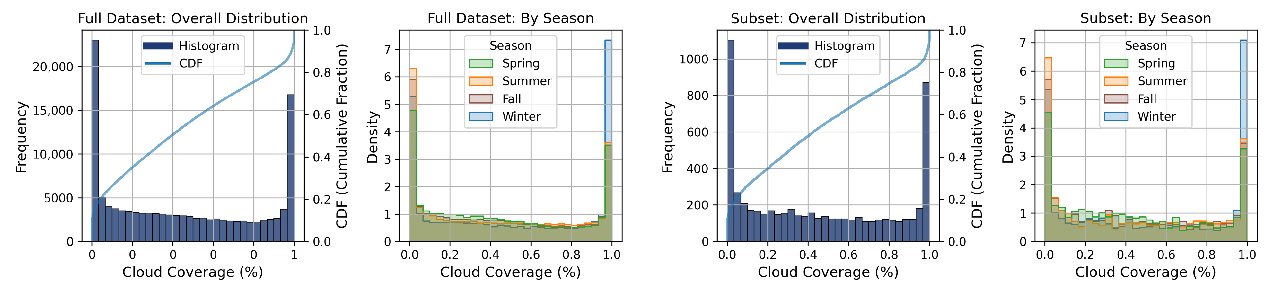
The SEN12MS-CR dataset is a publicly available, multimodal, global satellite, cloud-free dataset consisting of Sentinel-1 (SAR) imagery and Sentinel-2 imagery with cloudy/cloud-free pairs [9]. The dataset covers 175 regions of interest (ROIs) worldwide across different seasons and comprises a total of 122,218 256 × 256-pixel images. In this study, 6000 images were randomly sampled from this dataset, of which 5000 were allocated for training, 500 for validation, and another 500 for testing. To verify the representativeness of the subsets, the cloud cover distribution was calculated using the same statistical methods as the original dataset, as shown in Figure 5. The results indicate that the cloud cover distribution characteristics of the selected subsets are consistent with those of the full dataset.

The SMILE-CR dataset is a publicly available, multimodal, global, cloud-free dataset composed of Landsat-8 optical imagery, Sentinel-1 (SAR) imagery, and MODIS auxiliary imagery [11]. The dataset covers representative regions worldwide and comprises a total of 1400 images with a resolution of 512 × 256 pixels, of which 1000 images form the training set, while the validation and test sets each consist of 200 images. This paper retains the dataset’s original partitioning method.

For the preprocessing of the SEN12MS-CR data, the reference method provided by the dataset authors has been adopted by many other studies, and this paper follows that approach. Specifically, for the normalization of VV and VH polarizations in the Sentinel-1 (SAR) data, Equation (15) is used, which involves clipping the data followed by min-max normalization.

$$\begin{array}{cc}\hfill VV& ={\displaystyle \frac{clamp(VV,-25,0)-(-25)}{0-(-25)}}\hfill \\ \hfill VH& ={\displaystyle \frac{clamp(VH,-32.5,0)-(-32.5)}{0-(-32.5)}}\hfill \end{array}$$

(15)

For Sentinel-2 cloud-covered and cloud-free data, the values should be normalized by dividing them by 10,000 after cropping; see Equation (16) for reference.

$$\begin{array}{c}\hfill S2={\displaystyle \frac{clamp(S2,0,\mathrm{10,000})}{\mathrm{10,000}}}\end{array}$$

(16)

The SMILE-CR dataset was already normalized when it was provided, and this paper retains that normalization.

4.2. Experimental Settings and Evaluation Metrics

The experiments were conducted on the sample subsets described in Section 4.1, using an NVIDIA GeForce RTX 3090 (24 GB) for training. Training for both Stage 1 and Stage 2 was limited to a maximum of 100 epochs; if the PSNR metric on the validation set did not improve after 10 epochs, training was terminated. For the settings, the AdamW optimizer was used with a learning rate of $3\times {10}^{-5}$ and momentum parameters of (0.5, 0.9). The EMA smoothing coefficient for the codebook was set to 0.99, and the loss function weights were configured as described in Section 3.4. To better evaluate the impact of data volume under the two-stage framework, data augmentation was limited to random horizontal and vertical flipping.

Model performance is evaluated using four quantitative metrics: Mean Absolute Error (MAE), Spectral Angle Mapper (SAM), Peak Signal-to-Noise Ratio (PSNR), and Structural Similarity Index Measure (SSIM). Among these, MAE measures the average pixel-level deviation and SAM evaluates spectral consistency; both are pixel-level metrics. PSNR reflects the overall fidelity of the reconstructed image, while SSIM evaluates perceptual quality in terms of structure, brightness, and contrast. In the visualizations, SAR images use the VV polarization channel and Sentinel-2 optical images are presented in false-color form. All images undergo gamma correction with a coefficient of 0.7. Error maps are calculated based on the mean pixel error of each channel to visually illustrate prediction deviations.

4.3. Comparative Experiments

This paper compares the proposed model with SAR2OPT [20], SpA-GAN [18], McGAN [19], Dsen2-CR [22], Simulation-Fusion GAN [21], GLF-CR [23], HS2P [24], HPN-CR [25] and EMRDM [28]. On the SEN12MS-CR dataset, the SAR2OPT model uses only Sentinel-1 data, mapping it to Sentinel-2 data. SpA-GAN was originally designed for RGB channels; in this paper, we modified its input and output channels to accept Sentinel-2 data as input and output the same type of data, while other aspects remain consistent with the original paper. On the SMILE-CR dataset, for all models using a mosaicking approach as input, mosaicked MODIS data were added. For models using a branching method as input, MODIS data were additionally incorporated into the conditional branches. The number of parameters, FLOPs, inference time, and peak GPU memory consumption for each model are shown in

Table 1. Number of parameters, FLOPs, Time and GPU Memory for TCF-VQ GAN and other methods.

Method	Parameters (M)	FLOPs (G)	Time (ms)	GPU Mem (MB)
SAR2OPT	11.4	51.51	5.66	101.54
SpA GAN	0.2	15.53	12.12	110.59
McGAN	54.4	25.16	4.07	338.31
DSen2-CR	37.8	2478.13	173.34	4580.19
Simulation-Fusion GAN	83.7	13.13	1.35	363.49
GLF-CR	14.8	249.71	125.75	444.24
HS2P	21.4	1402.05	156.87	445.67
HPN-CR	3.6	17.69	38.27	123.26
EMRDM	39.1	662.14	271.82	1563.22
TCF-VQ GAN (Ours)	59.6	223.65	37.52	847.38

. The inference time is calculated as the average over 20 runs after 5 warm-up iterations. For diffusion-based models, the inference procedure is replaced by the sampling process, with the number of sampling steps kept consistent with the original settings in the corresponding papers. Quantitative experimental results are shown in

Table 2. Quantitative performance comparison of TCF-VQ GAN and other methods on SEN12MS-CR. Bold values indicate the best performance.

Method	Inputs		MAE↓	SAM↓	PSNR (dB)↑	SSIM↑
	OPT	SAR
SAR2OPT	×	✓	0.0424	11.6825	23.5399	0.7553
SpA-GAN	✓	×	0.0384	11.2119	23.8353	0.7981
McGAN	✓	✓	0.0345	9.4909	24.4685	0.8516
Simulation-Fusion GAN	✓	✓	0.0366	8.3789	25.2634	0.8551
DSen2-CR	✓	✓	0.0254	6.8623	25.9727	0.8843
GLF-CR	✓	✓	0.0226	6.6152	28.0119	0.8754
HS2P	✓	✓	0.0213	6.0845	29.1390	0.8995
HPN-CR	✓	✓	0.0196	5.7250	30.1964	0.9122
EMRDM	✓	✓	0.0300	7.7643	25.4122	0.8831
TCF-VQ GAN (Ours)	✓	✓	0.0165	4.7243	31.0397	0.9188

and

Table 3. Quantitative performance comparison of TCF-VQ GAN and other methods on SMILE-CR. Bold entries represent the best-performing results.

Method	Inputs			MAE↓	SAM↓	PSNR (dB)↑	SSIM↑
	OPT	SAR	MODIS
SAR2OPT	×	✓	✓	0.0316	6.8592	25.5241	0.7004
SpA-GAN	✓	×	×	0.0277	6.2425	24.8051	0.8254
McGAN	✓	✓	✓	0.0215	4.9348	28.5339	0.8562
Simulation-Fusion GAN	✓	✓	✓	0.0122	2.9536	31.2039	0.9028
DSen2-CR	✓	✓	✓	0.0151	4.2209	30.7857	0.8649
GLF-CR	✓	✓	✓	0.0131	3.2169	30.3482	0.8707
HS2P	✓	✓	✓	0.0111	2.6579	32.2900	0.9300
HPN-CR	✓	✓	✓	0.0169	3.7738	30.6296	0.8912
EMRDM	✓	✓	✓	0.0087	2.0618	32.9004	0.9325
TCF-VQ GAN (Ours)	✓	✓	✓	0.0082	2.1663	33.5191	0.9365

. In all tables, the arrows (↑/↓) indicate whether higher or lower values correspond to better performance, while checkmarks (✓) and crosses (×) denote whether the corresponding modality is used as input.

On the SEN12MS-CR dataset, TCF-VQ GAN achieved the best performance across all evaluation metrics, delivering state-of-the-art de-clouding performance. In terms of pixel-level error, TCF-VQ GAN achieved an MAE of 0.0196, a significant improvement over the 0.0165 achieved by HPN-CR. In terms of spectral consistency, TCF-VQ GAN achieved a SAM score of 4.7243, significantly outperforming other methods. Regarding image quality, TCF-VQ GAN achieved PSNR and SSIM scores of 31.0397 and 0.9188, respectively, representing significant improvements over both HPN-CR and EMRDM. It is worth noting that EMRDM performed poorly on the sample subsets used in this study; this may be because diffusion models cannot be adequately trained when the data is complex but the dataset is small. However, this model achieved good results on the SMILE-CR dataset. On the SMILE-CR dataset, leveraging the channel-space weighting capability of the SCGC module and the training strategy, the model effectively fused image data from three information sources, achieving the best performance on MAE, PSNR, and SSIM. Specifically, it achieved a PSNR of 33.5191, significantly outperforming EMRDM’s 32.9004.

In terms of model parameters, the proposed model maintains a parameter count at the average level of other methods. Compared to HS2P and Simulation-Fusion GAN, which have fewer parameters, the proposed method achieves optimal quantitative results while maintaining low FLOPs. It is worth noting that although the multi-branch structure used by HPN-CR maintains extremely low parameter counts and computational costs, its network design relies heavily on prior knowledge. It performs well when using only SAR as auxiliary data, but its performance deteriorates slightly when MODIS is further incorporated. Furthermore, as a diffusion model, EMRDM is significantly slower in inference than models based on CNNs or GANs.

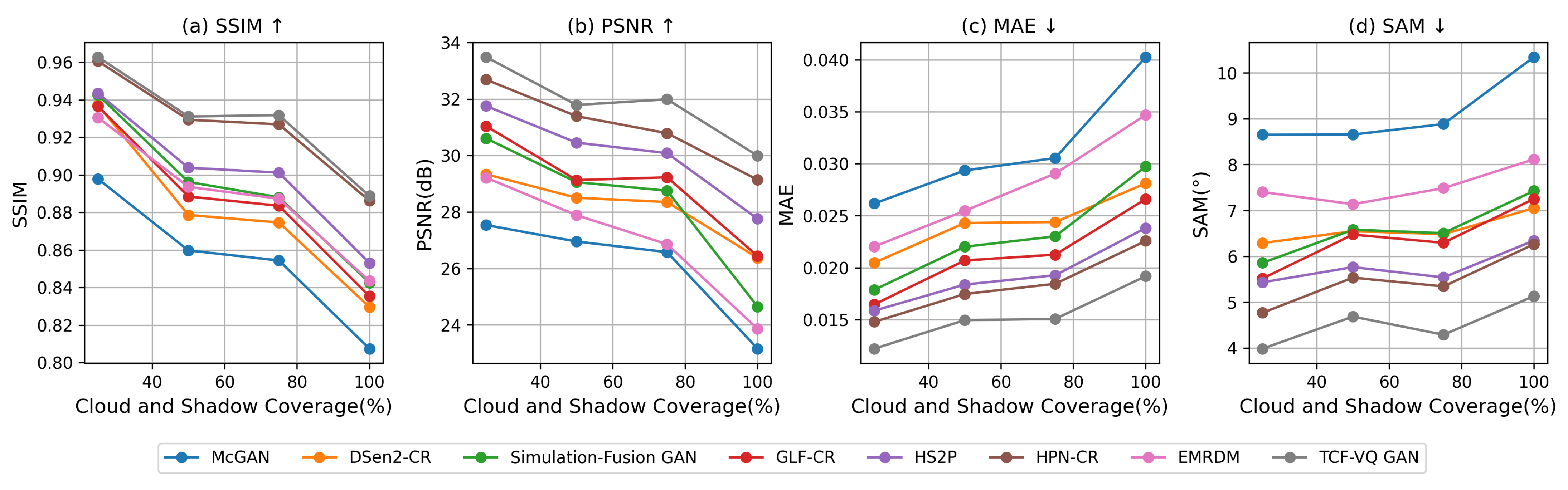
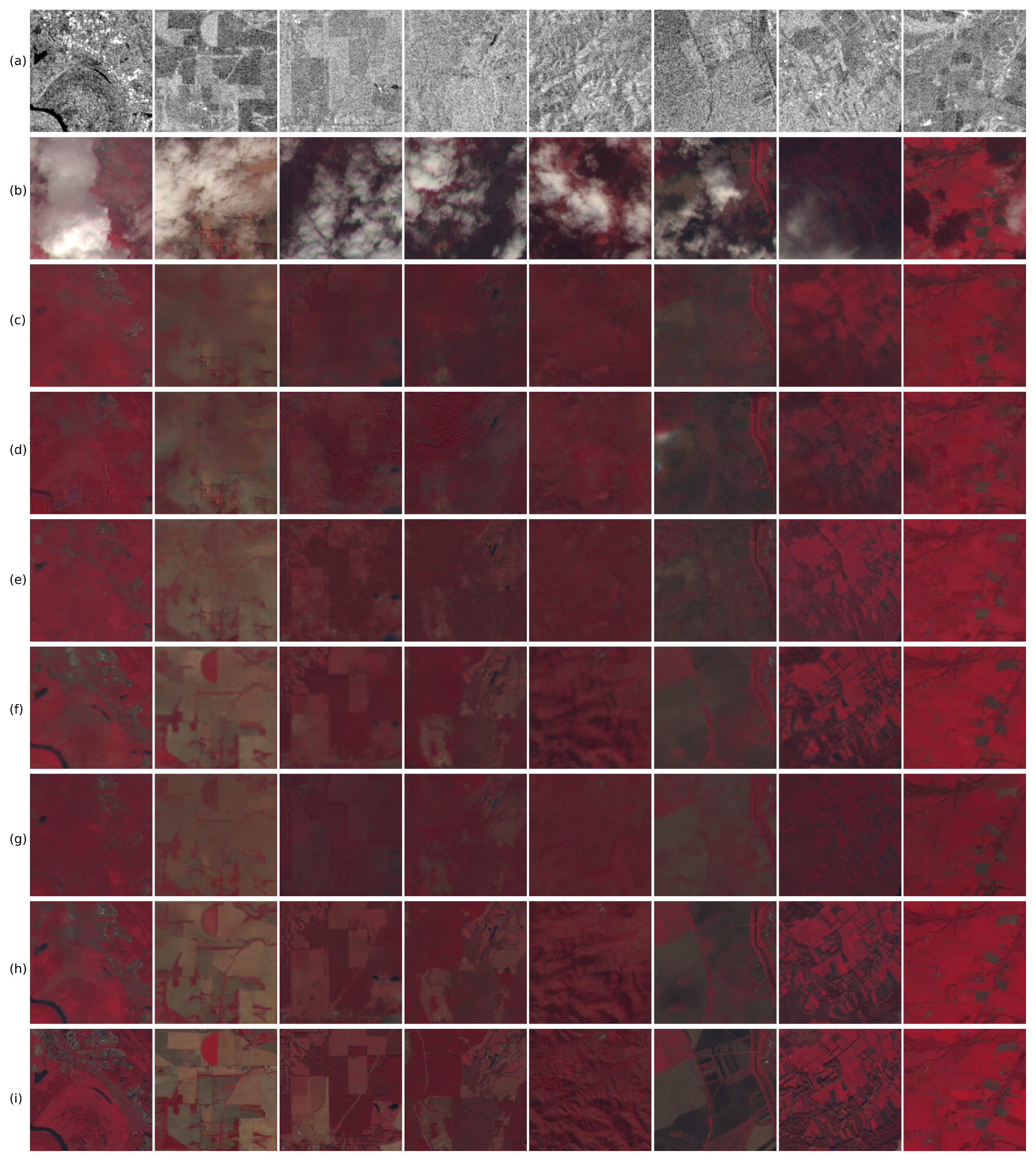
Furthermore, Figure 6 illustrates the trends in quantitative metrics on the SEN12MS-CR dataset as coverage varies, while Figure 7 demonstrates the prediction performance of major baseline models under different cloud and shadow coverage conditions.

As shown in Figure 6, the TCF-VQ GAN outperforms the previous state-of-the-art HPN-CR model across all metrics under various cloud and shadow coverage conditions. For all cloud coverage scenarios, the SSIM scores of the two models are relatively close. However, when cloud coverage exceeds 50%, our model significantly outperforms HPN-CR in terms of PSNR; it also achieves the best results across all other metrics at all coverage levels. As shown in Figure 7, the TCF-VQ GAN significantly improves the overall visual quality, more fully restoring the details and structures of objects in cloud or shadow regions. In high-coverage samples, the TCF-VQ GAN effectively reconstructs river structures and restores high-frequency details in thin cloud regions, yielding clearer and more complete results compared to those of HS2P and HPN-CR. In medium-coverage samples, TCF-VQ GAN produces sharper edges with fewer blurring artifacts. In low-coverage samples, TCF-VQ GAN’s reconstruction in shadowed areas closely resembles real imagery, featuring clear edges and accurate contrast, whereas HS2P remains affected by shadowing.

4.4. Two-Stage Training Framework

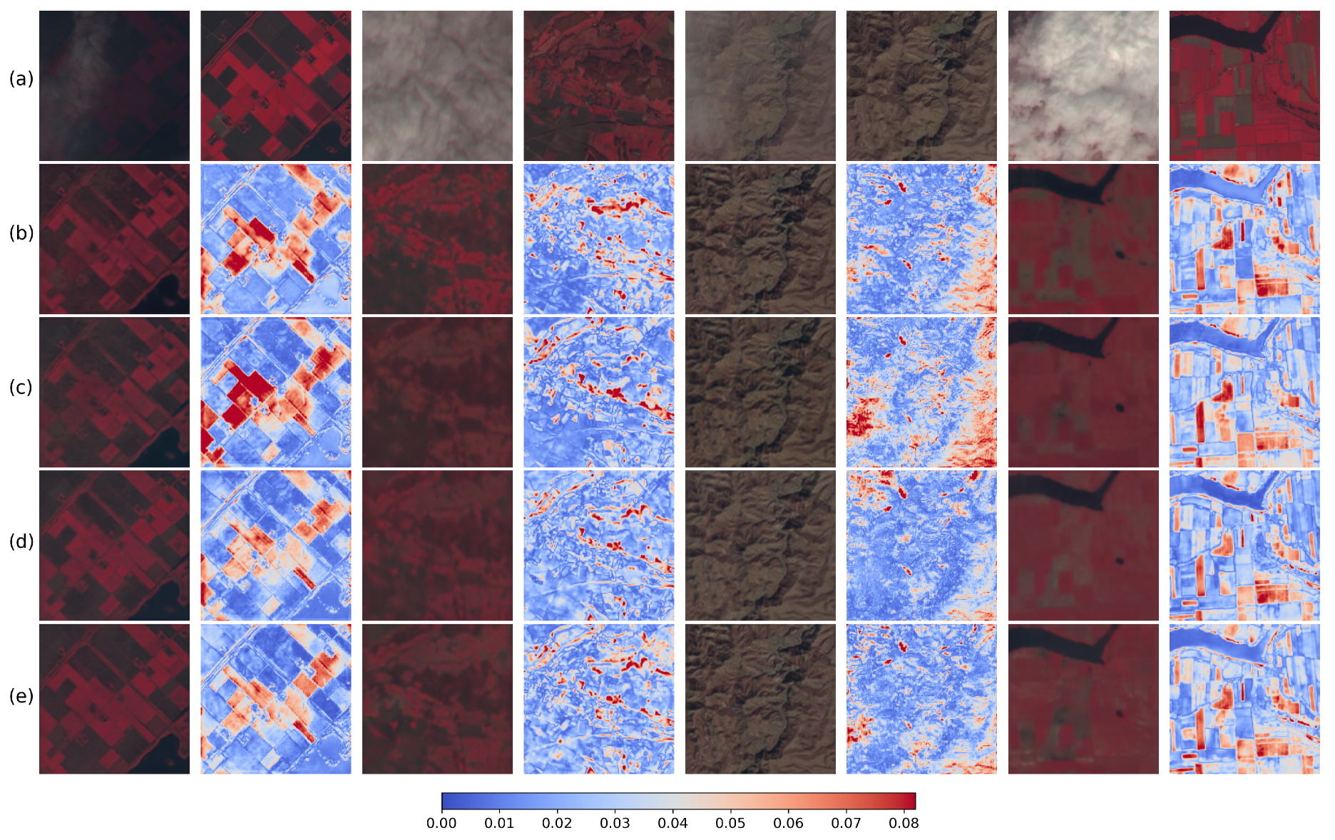
To address the issue of missing paired data, this paper proposes a two-stage training method. For validation, we randomly sampled from 5000 training samples to construct three datasets, each used for Stage I pre-training, while keeping the paired data for Stage II fixed. This was done to verify the impact of the data volume in Stage I on the final reconstruction results; the quantitative results are shown in

Table 4. Validation of the effectiveness of the TCF-VQ GAN two-stage training framework. The best performance is highlighted in bold.

STAGE I (Samples)	STAGE II (Samples)	MAE↓	SAM↓	PSNR (dB)↑	SSIM↑
0	1250	0.0232	6.5246	28.1487	0.8976
1250	1250	0.0238	6.7594	27.5579	0.8948
2500	1250	0.0230	6.4782	28.4470	0.8994
5000	1250	0.0228	6.3288	27.6908	0.9000
0	2500	0.0202	5.7497	29.5806	0.9079
2500	2500	0.0199	5.6646	29.7411	0.9091
5000	2500	0.0194	5.5557	29.8526	0.9098

. To more intuitively demonstrate the performance improvement, Figure 8 compares the prediction results and error plots for Stage I under different settings when Stage II uses 1250 paired data points, as shown in Table 4.

The results in Table 4 show that adjusting the pre-training data for Stage I can improve model performance while keeping Stage II data fixed. It can be seen that when the number of paired data sets in Stage II is fixed at 2, the SAM score differs by 0.194 between the no-pre-training case and the case where Stage I training uses 5000 cloud-free images. Specifically, Figure 8 further illustrates the impact of increasing only the Stage I data on the results when the number of paired data sets in Stage II is fixed at 1250. As shown in the first column of data, both the absolute error and visual performance improve significantly as the amount of pre-training data increases. Additionally, the model training in this paper stops when the PSNR shows no improvement for 10 consecutive iterations; in practice, it can be observed that the Stage II model requires more iterations to achieve optimal performance.

4.5. Ablation Study

To verify the impact of each design component on the performance of remote sensing image cloud removal, this section conducts ablation studies on the SCGC module design and the contributions of various loss functions. The quantitative results are shown in

Table 5. Convolution block and attention ablation experiments. Bold values indicate the best results.

Convolution	Attention	MAE↓	SAM↓	PSNR (dB)↑	SSIM↑
Gated	DCT	0.0200	5.7406	29.4416	0.9060
Residual	DCT	0.0192	5.3097	28.6635	0.9119
Residual	SE	0.0193	5.5875	29.9208	0.9093
Gated	SE	0.0165	4.7243	31.0397	0.9188

and

Table 6. Ablation studies of different terms in the loss function. The best results are shown in bold.

$\mathcal{L}$	MAE↓	SAM↓	PSNR (dB)↑	SSIM↑
w/o ${\mathcal{L}}_{SSIM}$	0.0229	6.7859	28.7909	0.8883
w/o ${\mathcal{L}}_{D{W}^{2}A}$	0.0171	4.9808	30.8497	0.9167
Full Loss	0.0165	4.7243	31.0397	0.9188

.

Table 5 presents the quantitative results when the convolutional blocks in the SCGC module are replaced with standard residual blocks or when the attention mechanism is replaced with a DCT channel attention mechanism. Figure 9 displays the features and gating values obtained during a single forward pass after training. Quantitative metrics indicate that the performance of the module using the SE attention mechanism is significantly superior to that of the module using the DCT attention mechanism. Furthermore, the visualization results of the forward pass demonstrate that across all downsampling levels, the gating values exhibit significant enhancement or suppression capabilities for cloud regions.

Table 6 shows the impact of including or excluding SSIM and DW²A in the loss function on the experimental results. It can be seen that removing either of these terms from the loss function has a significant effect on the results; in particular, removing DW²A leads to a substantial decrease in PSNR.

5. Discussion

Building on the experimental results and conclusions presented earlier, this section further discusses issues related to the de-clouding task addressed in this paper: (1) the improvement in model performance achieved by adding modalities; (2) changes in discrete codebook representations following pre-training and fusion fine-tuning; and (3) the limitations of loss functions based on cloud masks.

5.1. Analysis of the Impact of Training with Different Modality Combinations on Model Metrics

For deep learning models, under reasonable network design, adding data from the same source or the same modality typically does not degrade qualitative or quantitative metrics. However, multi-source or multi-modal data impose higher demands on network design. In this paper, we trained models using the SEN12MS-CR dataset (two-source) and the SMILE-CR dataset (three-source) without altering the model architecture. Therefore, it is necessary to discuss the improvement in model performance achieved by incorporating data from different modalities.

Table 7. Model metrics on the SMILE-CR dataset when using different modalities as input. Bold text highlights the best results.

Modalities			MAE↓	SAM↓	PSNR (dB)↑	SSIM↑
MS	SAR	MODIS
✓	×	×	0.0168	3.9605	28.3733	0.9069
✓	✓	×	0.0126	2.5662	29.9406	0.9241
✓	×	✓	0.0090	2.1876	32.5947	0.9271
✓	✓	✓	0.0082	2.1663	33.5191	0.9365

shows the changes in model metrics when trained on the SMILE-CR dataset using four different input combinations: multispectral data only, multispectral + SAR, multispectral + MODIS, and multispectral + SAR + MODIS. It can be observed that as the number of input modalities increases, all evaluation metrics of the model show a significant trend toward improvement. When using only multispectral (MS) single-modality input, the model’s performance was relatively poor compared to the baseline, with the highest MAE (0.0168) and the lowest PSNR (28.3733 dB). However, when SAR or MODIS modalities were introduced to form dual-modality inputs, performance improved significantly. Specifically, the MS+SAR combination reduced MAE to 0.0126 and and PSNR to 29.9406 dB, while the MS+MODIS combination showed even more pronounced gains, with MAE further reduced to 0.0090 and PSNR surging to 32.5947 dB. This indicates that both auxiliary modalities effectively supplement the key information missing from MS and that MODIS provides a relatively greater marginal contribution in this task. When all three modalities (MS, SAR, and MODIS) are used as inputs, the model achieves optimal performance, with MAE, PSNR, and SSIM reaching peak values of 0.0082, 33.5191 dB, and 0.9365, respectively. This progressive improvement in performance fully demonstrates that there is a certain degree of complementarity among different modal data. By reasonably fusing multi-source heterogeneous information, the model can capture richer and more robust feature representations, thereby achieving improvements in quantitative metrics. At the same time, this also confirms that the model proposed in this paper can effectively fuse multi-source data through its modular composition alone, without modifying the model architecture or designing additional conditional input fusion heads.

5.2. Analysis of Codebook Status After Two-Stage Training

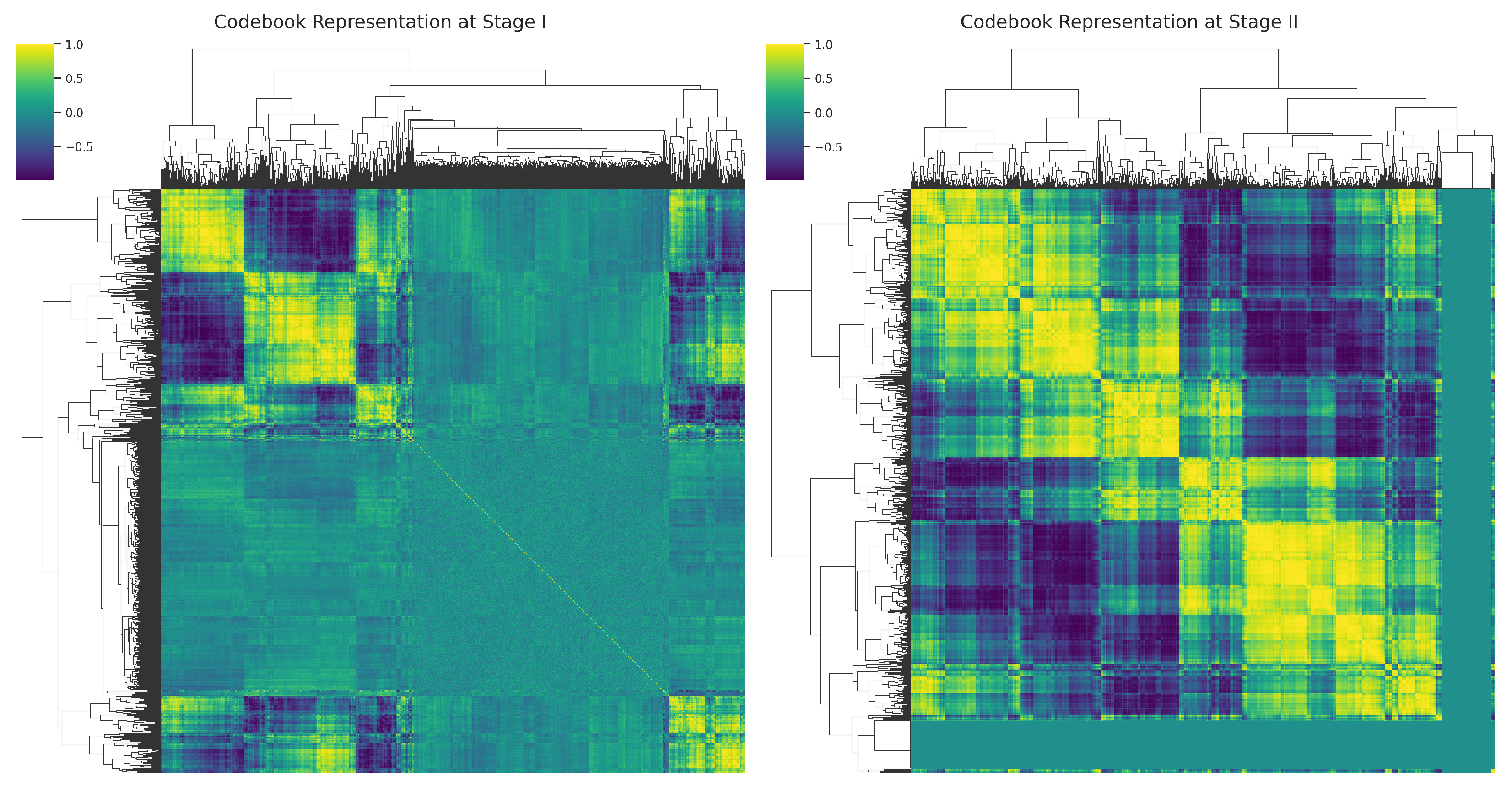
To further analyze the impact of the two-stage training strategy on the model’s internal feature representations, this paper visualizes and performs similarity analysis on the discrete codebooks obtained after each training stage. Specifically, we calculate the cosine similarity between embedding vectors in the codebook and plot the similarity matrix using hierarchical clustering to investigate the organizational structure of different codewords in the latent space, as shown in Figure 10.

During the unsupervised pre-training stage (Stage I), the codebook similarity matrix exhibits a relatively coarse-grained, block-like structure, revealing two dominant high-similarity clusters. Within each cluster, similarity is high and distribution is relatively uniform, while differences between clusters are distinct. This indicates that the model has developed preliminary semantic aggregation capabilities and is able to learn common features of land cover types, texture patterns, and degradation patterns. However, the latent space at this stage still exhibits some heterogeneity, with category boundaries not yet sufficiently defined. The code words tend to represent global trends, and their ability to capture local details and fine-grained differences remains limited. During the supervised fine-tuning stage (Stage II), the code book structure was further refined: the original large clusters were split into multiple subclusters, resulting in richer hierarchical relationships and clearer division of labor among codes, indicating that the supervisory signal enhanced the latent space’s discriminative power and stable mapping capability. At the same time, signs of degradation can be observed in a small number of entries, suggesting that some code words may exhibit low activity or representational collapse. While this phenomenon does not alter the overall trend of “enhanced refinement”, it indicates that Stage II, while improving separability, may still be accompanied by issues of uneven utilization of local code words.

Overall, the two-stage training process enables the model’s representational capabilities to evolve from general feature extraction to fine-grained semantic representations. Stage I focuses on learning the common structural characteristics of objects and their multimodal integration relationships; Stage II further optimizes the latent space through supervisory signals, enabling the model to exhibit greater sensitivity and accuracy in distinguishing variations in cloud thickness, shadows, and textures. It is evident that the two-stage training strategy effectively promotes the evolution of the latent space from coarse clustering to fine-grained differentiation, enhancing the separability and organization of the codebook.

5.3. Limitations of Cloud-Mask-Based Loss Functions

As seen in the previous section, the cloud removal task requires not only the removal of cloud layers but also the preservation of texture in cloud-free regions without distortion. An intuitive approach is to introduce a cloud mask into the loss function, enabling the model to learn separately for cloud and cloud-free regions. However, in practice, the accuracy of this method is highly dependent on the precision of the cloud mask calculation; therefore, a cloud mask-based loss function is not the optimal choice.

Among the models compared in this paper, DSen2-CR employs a cloud mask-based loss function, as shown in Equation (17):

$$\begin{array}{cc}\hfill {\mathcal{L}}_{CARL}=& {\displaystyle \frac{{\Vert CSM\odot (P-T)+(1-CSM)\odot (P-I)\Vert }_1}{N_{tot}}}\hfill \\ \hfill & +\lambda {\displaystyle \frac{{\Vert P-I\Vert }_1}{N_{tot}}}\hfill \end{array}$$

(17)

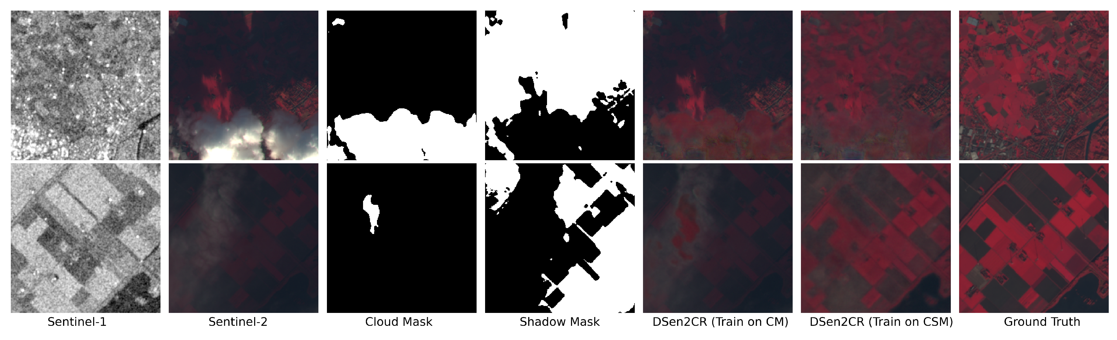
Here, CSM refers to the Binary Cloud and Cloud-shadow Mask. Although existing algorithms can generate masks with reasonable accuracy, their precision still directly impacts model performance when incorporated into the loss function. Figure 6 shows that under low cloud cover conditions, DSen2-CR does indeed outperform earlier models; however, the PSNR metric still exhibits a decline as cloud cover decreases. This is because in scenes with sparse clouds and abundant shadows, the algorithm’s ability to effectively identify shadowed regions becomes critical. If shadows are detected, the first term of the loss function guides the model to enhance the reconstruction of shadowed regions; if not detected, the first term degenerates into a direct loss for the shadowed image. The sample in the sixth column of row 6 in Figure 6d illustrates the model’s difficulty in effectively reconstructing images under complex cloud shadow conditions.

Figure 11 shows the simulation results after removing shadow detection from the DSen2-CR model. It can be seen that the network still performs well in removing cloud layers, but it barely processes the shadowed areas. Although the loss function includes a shadow mask, some thin clouds remain in the reconstruction results because the thin clouds in the right-hand region of the second row were neither identified by the shadow detector nor captured by the cloud detector. This further illustrates that the effectiveness of such loss functions depends on the accuracy of the mask. This paper addresses this issue in the model architecture by implementing feature selection through model design. Reviewing prior work, GLF-CR and HS2P also did not adopt mask-based loss functions; instead, they employed conditional or multi-channel attention mechanisms in their model design to perform dynamic feature filtering.

6. Conclusions

This paper proposes a GAN model based on TCF-VQ and designs a two-stage training framework: in the first stage, unsupervised training is performed using SAR/MODIS and cloud-free images to learn a discrete codebook, enabling preliminary reconstruction of sparse-cloud or low-light images and providing basic information fusion capabilities; in the second stage, supervised training is conducted using SAR/MODIS and cloud-covered images to further improve cloud removal performance. The model integrates an SCGC module for feature suppression and enhancement in both spatial and channel dimensions. To address the challenge of directly applying traditional perceptual loss functions to multispectral images, this paper proposes a multiscale self-weighted loss function, DW²A, based on the wavelet transform. Experiments conducted on subsets of SEN12MS-CR dataset and SMILE-CR demonstrate that the proposed method achieves state-of-the-art performance in both quantitative metrics and visual quality, particularly exhibiting higher fidelity under thick cloud conditions. Ablation experiments validate the effectiveness of this two-stage framework, showing that simply increasing the scale of unpaired data in the first stage can significantly improve performance. This paper analyzed how incorporating different modalities of data leads to an overall improvement in model performance, examined changes in latent spatial representations during pretraining and fusion fine-tuning, and pointed out that cloud mask-based loss function design is constrained by mask accuracy. Overall, the cloud removal algorithm integrates multi-task capabilities such as defogging, low-light enhancement, and conditional generation. Future research will explore the method’s generalization ability across different datasets, draw inspiration from model design approaches in other fields, and incorporate multi-temporal data to improve reconstruction quality and visual performance in complex cloud scenes.

References

1. King, M.D.; Platnick, S.; Menzel, W.P.; Ackerman, S.A.; Hubanks, P.A. Spatial and Temporal Distribution of Clouds Observed by MODIS Onboard the Terra and Aqua Satellites. IEEE Trans. Geosci. Remote Sens. 2013, 51, 3826–3852. [Google Scholar] [CrossRef]
2. Zhu, X.; Gao, F.; Liu, D.; Chen, J. A Modified Neighborhood Similar Pixel Interpolator Approach for Removing Thick Clouds in Landsat Images. IEEE Geosci. Remote Sens. Lett. 2012, 9, 521–525. [Google Scholar] [CrossRef]
3. Li, X.; Shen, H.; Zhang, L.; Zhang, H.; Yuan, Q.; Yang, G. Recovering Quantitative Remote Sensing Products Contaminated by Thick Clouds and Shadows Using Multitemporal Dictionary Learning. IEEE Trans. Geosci. Remote Sens. 2014, 52, 7086–7098. [Google Scholar] [CrossRef]
4. Xu, M.; Jia, X.; Pickering, M.; Plaza, A.J. Cloud Removal Based on Sparse Representation via Multitemporal Dictionary Learning. IEEE Trans. Geosci. Remote Sens. 2016, 54, 2998–3006. [Google Scholar] [CrossRef]
5. Meng, F.; Yang, X.; Zhou, C.; Li, Z. A Sparse Dictionary Learning-Based Adaptive Patch Inpainting Method for Thick Clouds Removal from High-Spatial Resolution Remote Sensing Imagery. Sensors 2017, 17, 2130. [Google Scholar] [CrossRef]
6. Zi, Y.; Xie, F.; Zhang, N.; Jiang, Z.; Zhu, W.; Zhang, H. Thin Cloud Removal for Multispectral Remote Sensing Images Using Convolutional Neural Networks Combined With an Imaging Model. IEEE J. Sel. Top. Appl. Earth Obs. Remote Sens. 2021, 14, 3811–3823. [Google Scholar] [CrossRef]
7. Zhang, H.; Xu, H.; Tian, X.; Jiang, J.; Ma, J. Image Fusion Meets Deep Learning: A Survey and Perspective. Inf. Fusion 2021, 76, 323–336. [Google Scholar] [CrossRef]
8. Bamler, R. Principles Of Synthetic Aperture Radar. Surv. Geophys. 2000, 21, 147–157. [Google Scholar] [CrossRef]
9. Ebel, P.; Meraner, A.; Schmitt, M.; Zhu, X.X. Multisensor Data Fusion for Cloud Removal in Global and All-Season Sentinel-2 Imagery. IEEE Trans. Geosci. Remote Sens. 2021, 59, 5866–5878. [Google Scholar] [CrossRef]
10. Ebel, P.; Xu, Y.; Schmitt, M.; Zhu, X.X. SEN12MS-CR-TS: A Remote-Sensing Data Set for Multimodal Multitemporal Cloud Removal. IEEE Trans. Geosci. Remote Sens. 2022, 60, 5222414. [Google Scholar] [CrossRef]
11. Xia, Y.; He, W.; Huang, Q.; Yin, G.; Liu, W.; Zhang, H. CRformer: Multi-modal Data Fusion to Reconstruct Cloud-Free Optical Imagery. Int. J. Appl. Earth Obs. Geoinf. 2024, 128, 103793. [Google Scholar] [CrossRef]
12. Kingma, D.P.; Welling, M. Auto-Encoding Variational Bayes. arXiv 2022, arXiv:1312.6114. [Google Scholar] [CrossRef]
13. van den Oord, A.; Vinyals, O.; Kavukcuoglu, K. Neural Discrete Representation Learning. arXiv 2018, arXiv:1711.00937. [Google Scholar] [CrossRef]
14. Esser, P.; Rombach, R.; Ommer, B. Taming Transformers for High-Resolution Image Synthesis. arXiv 2021, arXiv:2012.09841. [Google Scholar] [CrossRef]
15. Goodfellow, I.J.; Pouget-Abadie, J.; Mirza, M.; Xu, B.; Warde-Farley, D.; Ozair, S.; Courville, A.; Bengio, Y. Generative Adversarial Nets. In Proceedings of the Advances in Neural Information Processing Systems; Curran Associates, Inc.: Red Hook, NY, USA, 2014; Volume 27. [Google Scholar]
16. Mirza, M.; Osindero, S. Conditional Generative Adversarial Nets. arXiv 2014, arXiv:1411.1784. [Google Scholar] [CrossRef]
17. Zhu, J.Y.; Park, T.; Isola, P.; Efros, A.A. Unpaired Image-to-Image Translation Using Cycle-Consistent Adversarial Networks. In Proceedings of the 2017 IEEE International Conference on Computer Vision (ICCV), Venice; IEEE: Piscataway, NJ, USA, 2017; pp. 2242–2251. [Google Scholar] [CrossRef]
18. Pan, H. Cloud Removal for Remote Sensing Imagery via Spatial Attention Generative Adversarial Network. arXiv 2020, arXiv:2009.13015. [Google Scholar] [CrossRef]
19. Enomoto, K.; Sakurada, K.; Wang, W.; Fukui, H.; Matsuoka, M.; Nakamura, R.; Kawaguchi, N. Filmy Cloud Removal on Satellite Imagery with Multispectral Conditional Generative Adversarial Nets. In Proceedings of the 2017 IEEE Conference on Computer Vision and Pattern Recognition Workshops (CVPRW); IEEE: Piscataway, NJ, USA, 2017; pp. 1533–1541. [Google Scholar] [CrossRef]
20. Bermudez, J.D.; Happ, P.N.; Oliveira, D.A.B.; Feitosa, R.Q. Sar to optical image synthesis for cloud removal with generative adversarial networks. ISPRS Ann. Photogramm. Remote. Sens. Spat. Inf. Sci. 2018, IV-1, 5–11. [Google Scholar] [CrossRef]
21. Gao, J.; Yuan, Q.; Li, J.; Zhang, H.; Su, X. Cloud Removal with Fusion of High Resolution Optical and SAR Images Using Generative Adversarial Networks. Remote Sens. 2020, 12, 191. [Google Scholar] [CrossRef]
22. Meraner, A.; Ebel, P.; Zhu, X.X.; Schmitt, M. Cloud Removal in Sentinel-2 Imagery Using a Deep Residual Neural Network and SAR-optical Data Fusion. ISPRS J. Photogramm. Remote Sens. 2020, 166, 333–346. [Google Scholar] [CrossRef]
23. Xu, F.; Shi, Y.; Ebel, P.; Yu, L.; Xia, G.S.; Yang, W.; Zhu, X.X. GLF-CR: SAR-enhanced Cloud Removal with Global–Local Fusion. ISPRS J. Photogramm. Remote Sens. 2022, 192, 268–278. [Google Scholar] [CrossRef]
24. Li, Y.; Wei, F.; Zhang, Y.; Chen, W.; Ma, J. HS2P: Hierarchical Spectral and Structure-Preserving Fusion Network for Multimodal Remote Sensing Image Cloud and Shadow Removal. Inf. Fusion 2023, 94, 215–228. [Google Scholar] [CrossRef]
25. Gu, P.; Liu, W.; Feng, S.; Wei, T.; Wang, J.; Chen, H. HPN-CR: Heterogeneous Parallel Network for SAR-Optical Data Fusion Cloud Removal. IEEE Trans. Geosci. Remote Sens. 2025, 63, 5402115. [Google Scholar] [CrossRef]
26. Jing, R.; Duan, F.; Lu, F.; Zhang, M.; Zhao, W. Denoising Diffusion Probabilistic Feature-Based Network for Cloud Removal in Sentinel-2 Imagery. Remote Sens. 2023, 15, 2217. [Google Scholar] [CrossRef]
27. Zou, X.; Li, K.; Xing, J.; Zhang, Y.; Wang, S.; Jin, L.; Tao, P. DiffCR: A Fast Conditional Diffusion Framework for Cloud Removal From Optical Satellite Images. IEEE Trans. Geosci. Remote Sens. 2024, 62, 5612014. [Google Scholar] [CrossRef]
28. Liu, Y.; Li, W.; Guan, J.; Zhou, S.; Zhang, Y. Effective Cloud Removal for Remote Sensing Images by an Improved Mean-Reverting Denoising Model with Elucidated Design Space. In Proceedings of the IEEE/CVF Conference on Computer Vision and Pattern Recognition; IEEE: Piscataway, NJ, USA, 2025; pp. 17851–17861. [Google Scholar]
29. Bengio, Y.; Léonard, N.; Courville, A. Estimating or Propagating Gradients Through Stochastic Neurons for Conditional Computation. arXiv 2013, arXiv:1308.3432. [Google Scholar] [CrossRef]
30. Xia, M.; Jia, K. Reconstructing Missing Information of Remote Sensing Data Contaminated by Large and Thick Clouds Based on an Improved Multitemporal Dictionary Learning Method. IEEE Trans. Geosci. Remote Sens. 2022, 60, 5605914. [Google Scholar] [CrossRef]
31. Ling, J.; Zhang, H. WCDL: A Weighted Cloud Dictionary Learning Method for Fusing Cloud-Contaminated Optical and SAR Images. IEEE J. Sel. Top. Appl. Earth Obs. Remote Sens. 2023, 16, 2931–2941. [Google Scholar] [CrossRef]
32. Wang, Z.; Zhang, J.; Chen, R.; Wang, W.; Luo, P. RestoreFormer: High-Quality Blind Face Restoration from Undegraded Key-Value Pairs. In Proceedings of the 2022 IEEE/CVF Conference on Computer Vision and Pattern Recognition (CVPR), New Orleans, LA, USA, 2022; IEEE: Piscataway, NJ, USA, 2022; pp. 17491–17500. [Google Scholar] [CrossRef]
33. Wang, Z.; Zhang, J.; Chen, T.; Wang, W.; Luo, P. RestoreFormer++: Towards Real-World Blind Face Restoration from Undegraded Key-Value Pairs. arXiv 2023, arXiv:2308.07228. [Google Scholar] [CrossRef]
34. Liu, L.; Chen, B.; Chen, H.; Zou, Z.; Shi, Z. Diverse Hyperspectral Remote Sensing Image Synthesis With Diffusion Models. IEEE Trans. Geosci. Remote Sens. 2023, 61, 5532616. [Google Scholar] [CrossRef]
35. Wang, M.; Song, Y.; Wei, P.; Xian, X.; Shi, Y.; Lin, L. IDF-CR: Iterative Diffusion Process for Divide-and-Conquer Cloud Removal in Remote-Sensing Images. IEEE Trans. Geosci. Remote Sens. 2024, 62, 5615014. [Google Scholar] [CrossRef]
36. Guu, K.; Hashimoto, T.B.; Oren, Y.; Liang, P. Generating Sentences by Editing Prototypes. arXiv 2018, arXiv:1709.08878. [Google Scholar] [CrossRef]
37. Liu, G.; Reda, F.A.; Shih, K.J.; Wang, T.C.; Tao, A.; Catanzaro, B. Image Inpainting for Irregular Holes Using Partial Convolutions. arXiv 2018, arXiv:1804.07723. [Google Scholar] [CrossRef]
38. Yu, J.; Lin, Z.; Yang, J.; Shen, X.; Lu, X.; Huang, T. Free-Form Image Inpainting With Gated Convolution. In Proceedings of the 2019 IEEE/CVF International Conference on Computer Vision (ICCV), Seoul, South Korea, 27 OCtober–2 November 2019; IEEE: Piscataway, NJ, USA, 2019; pp. 4470–4479. [Google Scholar] [CrossRef]
39. Hu, J.; Shen, L.; Sun, G. Squeeze-and-Excitation Networks. In Proceedings of the 2018 IEEE/CVF Conference on Computer Vision and Pattern Recognition, 2018; IEEE: Piscataway, NJ, USA, 2018; pp. 7132–7141. [Google Scholar] [CrossRef]
40. Qin, Z.; Zhang, P.; Wu, F.; Li, X. FcaNet: Frequency Channel Attention Networks. arXiv 2021, arXiv:2012.11879. [Google Scholar] [CrossRef]
41. Ma, J.; Tang, L.; Fan, F.; Huang, J.; Mei, X.; Ma, Y. SwinFusion: Cross-domain Long-range Learning for General Image Fusion via Swin Transformer. IEEE/CAA J. Autom. Sin. 2022, 9, 1200–1217. [Google Scholar] [CrossRef]
42. Vaswani, A.; Shazeer, N.; Parmar, N.; Uszkoreit, J.; Jones, L.; Gomez, A.N.; Kaiser, Ł.; Polosukhin, I. Attention Is All You Need. In Proceedings of the Advances in Neural Information Processing Systems; Guyon, I., Luxburg, U.V., Bengio, S., Wallach, H., Fergus, R., Vishwanathan, S., Garnett, R., Eds.; Curran Associates, Inc.: Red Hook, NY, USA, 2017; Volume 30. [Google Scholar]
43. Lee, J.; Lee, Y.; Kim, J.; Kosiorek, A.R.; Choi, S.; Teh, Y.W. Set Transformer: A Framework for Attention-based Permutation-Invariant Neural Networks. arXiv 2019, arXiv:1810.00825. [Google Scholar] [CrossRef]
44. Tolstikhin, I.O.; Houlsby, N.; Kolesnikov, A.; Beyer, L.; Zhai, X.; Unterthiner, T.; Yung, J.; Steiner, A.; Keysers, D.; Uszkoreit, J.; et al. MLP-Mixer: An All-MLP Architecture for Vision. In Proceedings of the Advances in Neural Information Processing Systems; Curran Associates, Inc.: Red Hook, NY, USA, 2021; Volume 34, pp. 24261–24272. [Google Scholar]
45. Ren, H.; Dai, H.; Dai, Z.; Yang, M.; Leskovec, J.; Schuurmans, D.; Dai, B. Combiner: Full Attention Transformer with Sparse Computation Cost. In Proceedings of the Advances in Neural Information Processing Systems; Ranzato, M., Beygelzimer, A., Dauphin, Y., Liang, P.S., Vaughan, J.W., Eds.; Curran Associates, Inc.: Red Hook, NY, USA, 2021; Volume 34, pp. 22470–22482. [Google Scholar]
46. Johnson, J.; Alahi, A.; Fei-Fei, L. Perceptual Losses for Real-Time Style Transfer and Super-Resolution. In Proceedings of the Computer Vision—ECCV 2016; Leibe, B., Matas, J., Sebe, N., Welling, M., Eds.; Springer International Publishing: Cham, Switzerland, 2016; pp. 694–711. [Google Scholar]
47. Mallat, S. A Theory for Multiresolution Signal Decomposition: The Wavelet Representation. IEEE Trans. Pattern Anal. Mach. Intell. 1989, 11, 674–693. [Google Scholar] [CrossRef]
48. Orea-Flores, I.Y.; Gallegos-Funes, F.J.; Arellano-Reynoso, A. Local Complexity Estimation Based Filtering Method in Wavelet Domain for Magnetic Resonance Imaging Denoising. Entropy 2019, 21, 401. [Google Scholar] [CrossRef]
49. Sharif, I.; Khare, S. Comparative Analysis of Haar and Daubechies Wavelet for Hyper Spectral Image Classification. Int. Arch. Photogramm. Remote Sens. Spat. Inf. Sci. 2014, XL-8, 937–941. [Google Scholar] [CrossRef]
50. Isola, P.; Zhu, J.Y.; Zhou, T.; Efros, A.A. Image-to-Image Translation with Conditional Adversarial Networks. arXiv 2018, arXiv:1611.07004. [Google Scholar] [CrossRef]
51. Wang, Z.; Bovik, A.; Sheikh, H.; Simoncelli, E. Image Quality Assessment: From Error Visibility to Structural Similarity. IEEE Trans. Image Process. 2004, 13, 600–612. [Google Scholar] [CrossRef] [PubMed]
Figure 1. Network architecture of TCF-VQ GAN under the two-stage training framework.
Remotesensing 18 01643 g001
Figure 2. Spatial-Channel Jointed Gated Convolution (SCGC) Module.
Remotesensing 18 01643 g002
Figure 3. Visualization of the computational process of convolution, partial convolution, and gated convolution.
Remotesensing 18 01643 g003
Figure 4. Computation flow of the DW2A Loss and visualization of its decomposition at each level.
Remotesensing 18 01643 g004
Figure 5. Overall and sampled subset distribution statistics of the SEN12MS-CR dataset.
Remotesensing 18 01643 g005
Figure 6. Effect of cloud and shadow coverage variations on the performance metrics of each model.
Remotesensing 18 01643 g006
Figure 7. Predicted results of different models under varying cloud coverage. From left to right, cloud coverage decreases: (a) SAR image; (b) cloudy image; (c) Simulation-Fusion GAN; (d) GLF-CR; (e) HS2P; (f) HPN-CR; (g) EMRDM; (h) TCF-VQ GAN; (i) ground truth.
Remotesensing 18 01643 g007
Figure 8. Comparison of results under the two-stage training framework with Stage II sample size fixed at 1250 images and varying Stage I training scales. Each pair of columns represents: (a) left—optical image and right—cloud-free reference and (be) results for no Stage I training and Stage I training with 1250, 2500, and 5000 samples, respectively.
Remotesensing 18 01643 g008
Figure 9. Visualization of gated convolution at different downsampling levels in a single forward pass.
Remotesensing 18 01643 g009
Figure 10. Visualization of the codebook embedding cosine similarity matrix after two-stage training using hierarchical clustering.
Remotesensing 18 01643 g010
Figure 11. Comparison of DSen2-CR results after manually removing shadow detection from the loss function. CM uses only cloud masks, while CSM combines cloud and shadow masks.
Remotesensing 18 01643 g011