GeoHybridGNN: A Hybrid Intelligent Mapping Framework for Porphyry Copper Prospectivity Mapping Integrating Remote Sensing, Geology, and Geochemistry

Highlights

What are the main findings?

• Proposes a geology-informed GeoHybridGNN framework for porphyry copper prospectivity mapping by integrating remote sensing, geochemical, structural, and graph-based neighborhood information with geological node attributes.
• Produces spatially coherent prospectivity maps and stable uncertainty patterns, with improved target delineation relative to the tested comparison models.

What are the implications of the main findings?

• Shows that hybrid integration of raster-based evidence and graph-based neighborhood learning with geological node attributes can support mineral exploration targeting in structurally complex porphyry systems.
• Provides an interpretable workflow combining prospectivity mapping, uncertainty estimation, and geochemical ablation analysis for exploration screening.

Abstract

The Western Chagai Belt of Pakistan hosts major porphyry Cu-Au systems, but prospectivity mapping in this arc remains difficult because favorable lithology, intrusive bodies, fault corridors, hydrothermal alteration, and Cu geochemical anomalies are spatially heterogeneous across a structurally complex and arid terrain. These conditions create a scientific need for an integrated mapping framework that can combine remote sensing alteration evidence, geology, structure, and geochemistry within a unified and reproducible workflow. This study presents GeoHybridGNN, a hybrid deep learning framework for porphyry copper prospectivity mapping in the Western Chagai Belt. The framework integrates multi-source raster evidence, including remote sensing-derived spectral alteration indices, a Cu geochemical raster, and distance-to-fault information, with graph-based node representations that combine regular neighborhood adjacency on retained grid cells with node attributes derived from lithology and aligned geoscientific raster summaries. All predictors were harmonized to a common 30 m reference raster grid and evaluated using five-fold spatial block cross-validation to provide a more spatially realistic assessment than ordinary random splitting. The implemented model combines a CNN-based raster patch encoder with a GraphSAGE-based graph classifier. Raster patches extracted around graph nodes are encoded into 64-dimensional embeddings, and these embeddings are concatenated with node-level graph features before full-batch graph learning and prediction. Copper occurrences were used only for supervised label assignment and evaluation and were not used as predictive inputs. The results show that GeoHybridGNN produces spatially coherent prospectivity maps, stable fold-wise prediction patterns, and improved target delineation relative to the tested comparison models. Cu geochemical integration produces only a limited change in global discrimination but provides modest local target sharpening in selected zones. These results indicate that GeoHybridGNN can serve as an uncertainty-aware and geologically constrained decision support workflow for porphyry copper targeting. More broadly, the framework provides a transparent strategy for exploration screening in structurally complex and data-heterogeneous metallogenic belts where remote sensing, geological, structural, and geochemical evidence must be integrated consistently.

1. Introduction

Porphyry copper deposits are among the most important sources of copper and associated metals. They remain a major focus of both research and mineral exploration because they can host very large resources and support long mine life. Regional assessments are useful for understanding metallogenic potential at broad scales, but exploration decisions usually require spatially explicit maps that can rank targets within a smaller and more practical area [1,2]. The Western Chagai Belt in Balochistan, Pakistan, is well-suited to this type of study. It forms part of the Tethyan metallogenic belt and includes major porphyry Cu-Au systems such as Reko Diq and Saindak. Recent studies from Pakistan further emphasize the importance of arc-related Cu-Au mineralization and tectono-magmatic evolution, including Cu-Au vein-type mineralization in the Kohistan arc and A-type intermediate-felsic magmatism in the NW Himalaya [3,4]. Although these examples are outside the Western Chagai Belt, they highlight the broader need to evaluate Pakistan’s metallogenic belts within an integrated tectonic, geological, and geochemical framework. The Western Chagai Belt also shows strong spatial variation in lithology, intrusive rocks, fault systems, alteration patterns, and geochemical anomalies. This complexity makes the region geologically important but difficult to evaluate using a single type of evidence. A practical targeting model, therefore, needs to integrate multiple data sources within a consistent spatial framework and produce results that are both predictive and geologically meaningful. Recent work on Pakistan’s mineral-resource data has also shown that multimodal large language models can support efficient extraction, harmonization, and integration of heterogeneous mineral-resource information, providing structured datasets that can complement AI-based prospectivity mapping workflows [5].

Mineral prospectivity mapping has developed from classical evidence integration and statistical favorability mapping to more flexible machine learning workflows. Early studies established the importance of quantitative evaluation, map performance assessment, and the systematic use of predictive evidence [6]. Later studies showed that machine learning methods, including random forests and logistic-based weighting, can improve prediction when geological and geochemical layers are integrated carefully [7,8]. More recent work has further advanced data-driven prospectivity analysis through hyperparameter optimization, interpretable frameworks, and improved workflow design [9,10]. At the same time, remote sensing and deep learning have expanded the data and modeling options available for mineral targeting. Multispectral data can capture lithological variation, alteration patterns, surface texture, and structural context, while deep neural networks can learn nonlinear spatial signatures from multi-layer inputs. Recent studies have shown strong performance of convolutional autoencoder and convolutional neural network approaches in mineral prospectivity mapping, and related remote sensing studies have confirmed the value of deep learning for lithological and alteration mapping from satellite data [11,12,13,14,15,16]. A recent review further indicates that deep learning is now a major direction in mineral prospectivity mapping, although important challenges remain in data preparation, validation, and interpretability [17,18,19,20].

However, important limitations remain. Raster-based convolutional models are effective for regular grid data, but they do not explicitly represent neighborhood relations among retained spatial units together with geological attributes such as lithology, raster-derived structural summaries, and distance-to-fault information. This has led to growing interest in graph neural networks for mineral prospectivity mapping. Recent studies show that graph-based learning can better capture spatial relations and mixed data structures, while multimodal fusion approaches are beginning to improve how different geological representations are combined [21,22]. At the same time, explainable artificial intelligence is becoming increasingly important because exploration models must do more than identify favorable areas. They must also support geological interpretation and decision-making [23]. Another major issue is model evaluation. In spatial prediction problems, random cross-validation can produce overly optimistic results when nearby training and test samples share similar spatial context. Spatially separated validation is therefore more realistic for mineral targeting. In addition, prospectivity results can be sensitive to the selection of non-deposit samples, uncertainty in the workflow, and the modeling choices used to produce the final map [24,25,26]. These issues are especially important in greenfield to brownfield exploration settings, where model stability and map reliability directly affect follow-up decisions. To address these issues, this study develops GeoHybridGNN, a geology-informed hybrid deep learning framework for porphyry copper prospectivity mapping in the Western Chagai Belt.

The framework integrates two complementary information streams. The first stream encodes raster-based evidence, including spectral alteration indices and a Cu geochemical raster. The second stream encodes graph-based node representations derived from lithology, aligned geoscientific raster summaries, and regular neighborhood adjacency on retained grid cells. These two streams are linked through a concatenation-based hybrid fusion mechanism, which allows the model to combine raster patterns and graph-based geological context within a unified prediction framework. All input layers were reprojected, quality checked, and aligned to a common 30 m grid before graph construction and feature extraction. Model evaluation was carried out using 5-fold spatial block cross-validation to reduce spatial leakage and provide a more realistic estimate of predictive performance. The final outputs include ensemble mean prospectivity maps, uncertainty maps expressed as fold-wise standard deviation, probability difference maps from Cu geochemical integration, and ROI hotspot maps for focused geological interpretation. This design moves the workflow beyond a single prediction surface and toward a more complete targeting system that can support practical exploration decisions.

The main contribution of this paper is twofold. First, it introduces the GeoHybridGNN architecture, which combines raster encoding, graph encoding, and concatenation-based hybrid fusion for porphyry copper targeting. Second, it presents a block-based spatially evaluated and uncertainty-aware prospectivity workflow for the Western Chagai Belt that is built directly from multi-source geological, structural, remote sensing, and geochemical evidence. The study shows how this combination can improve spatial coherence, interpretability, and targeting value in a region where mineralization is controlled by both regional tectonic structure and local geological complexity.

The remainder of the paper is organized as follows. Section 2 describes the study area and geological setting. Section 3 presents the data and methods, including data inputs, preprocessing, graph construction, the GeoHybridGNN architecture, concatenation-based hybrid fusion, and the 5-fold spatial block cross-validation design. Section 4 presents the results. Section 5 discusses the geological significance and modeling implications of the results. Section 6 concludes the study.

2. Study Area and Regional Tectonic Framework

The study area is located in the Western Chagai Belt of Balochistan, Pakistan, within the broader Chagai magmatic arc of the Tethyan metallogenic domain. It lies in the northwestern part of the country, close to the borders with Afghanistan and Iran, and covers the main zone where porphyry copper mineralization, major faults, tectonic boundaries, and favorable lithological units are spatially concentrated. This arc is one of the main porphyry copper provinces in western and southern Asia and extends westward toward Iran and Afghanistan. Previous regional assessments and deposit scale studies show that the Chagai belt contains a long-lived subduction-related magmatic system with strong porphyry copper fertility [2].

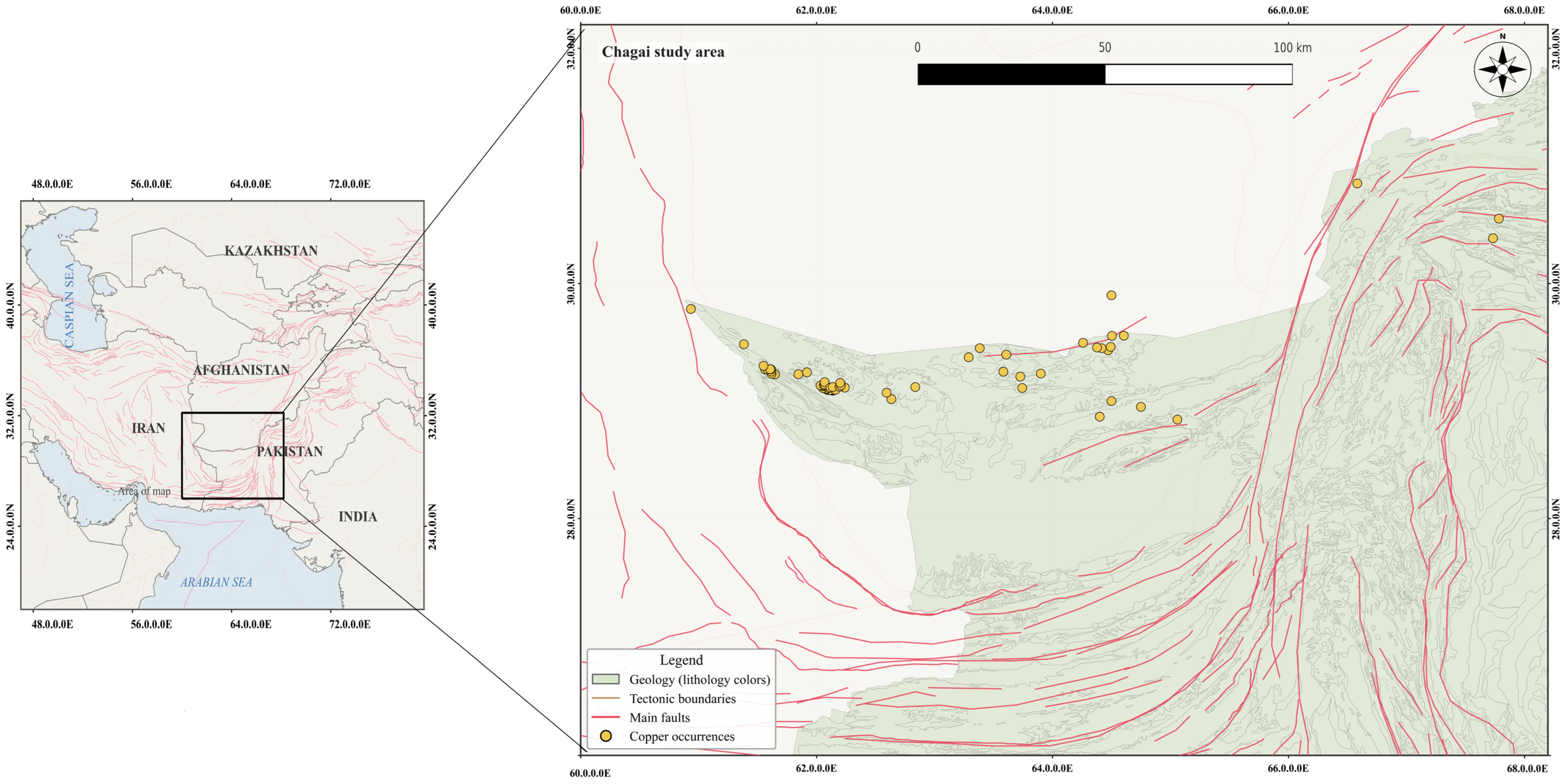
The Western Chagai Belt is the most relevant part of the arc for this study because it hosts the main known porphyry Cu-Au systems, including Reko Diq, Saindak, and several other prospects. This concentration of known mineral systems makes the area a suitable natural laboratory for prospectivity mapping. Figure 1 shows the regional location and internal spatial framework of the study area, including geology, tectonic boundaries, major faults, and mapped copper occurrences. The spatial distribution of these occurrences shows a close association with structurally controlled belts and favorable host units, which supports the use of an integrated spatial modeling framework.

The area is also favorable for remote sensing analysis because bedrock exposure is relatively good and vegetation sparse, which helps the detection of lithological and hydrothermal signals [27,28]. The selected study window, therefore, provides a suitable basis for prospectivity mapping because it captures both mineralized zones and surrounding non-mineralized areas needed for model learning, comparison, and prediction.

Geological Framework and Mineralization Controls

The Chagai arc is dominated by calc-alkaline to high-K calc-alkaline volcanic and intrusive rocks formed in an arc setting. The exposed units include andesitic to dacitic volcanic rocks, volcaniclastic sequences, and intrusive bodies ranging from diorite and quartz diorite to tonalite and granodiorite. These rocks record repeated magmatic activity and provide the main host environment for porphyry-style mineralization in the belt [29,30,31]. In the Western Chagai Belt, mineralized centers are commonly associated with small porphyry stocks, multiphase intrusions, and intrusive volcanic contacts. These features are important because porphyry systems typically form where magmatism, structure, and favorable host rocks interact in a focused way. Regional faults, fracture corridors, and intrusive margins therefore play a major role in magma ascent, fluid flow, and ore deposition. Recent work in the belt also shows that concealed and partly covered targets can preserve clear geophysical, geochemical, and alteration signatures, as demonstrated at Siah Diq [32]. Hydrothermal alteration in the Western Chagai Belt is typical of porphyry Cu-Au systems. Reported alteration styles include potassic, phyllic, argillaceous, and propylitic assemblages, together with quartz veining, stockwork development, sulfide mineralization, and local supergene overprint. At Saindak, for example, alteration and mineralization are zoned around ore-related porphyry intrusions, showing a clear link between tonalitic to dioritic magmatism and Cu, Au mineralization [29,30,33]. At the regional scale, these geological features are directly relevant to this study because they control the spatial distribution of favorable lithology, structural pathways, and alteration patterns.

Remote sensing and exploration studies have shown that alteration minerals and structural corridors can be mapped across large parts of the Western Chagai Belt and can help distinguish favorable zones from less prospective ground [27,28]. This is especially useful in the arid setting of the study area, where hydrothermal signatures are often well- preserved at the surface. The geological setting of the Western Chagai Belt directly supports the modeling framework used in this study. Lithology and geological contacts provide information on host rocks and intrusive context. Faults and tectonic boundaries represent major pathways and structural controls for magmatic hydrothermal fluids [34]. Spectral indices are relevant because alteration minerals are widespread and commonly exposed at the surface. Distance to fault captures proximity to major structural corridors, while the Cu geochemical raster reflects mineralization-related enrichment. For these reasons, a hybrid framework that combines raster-based information with graph-based neighborhood representation and geological node attributes is well-suited to prospectivity mapping in the Western Chagai Belt.

3. Data and Methods

3.1. Overview of GeoHybridGNN

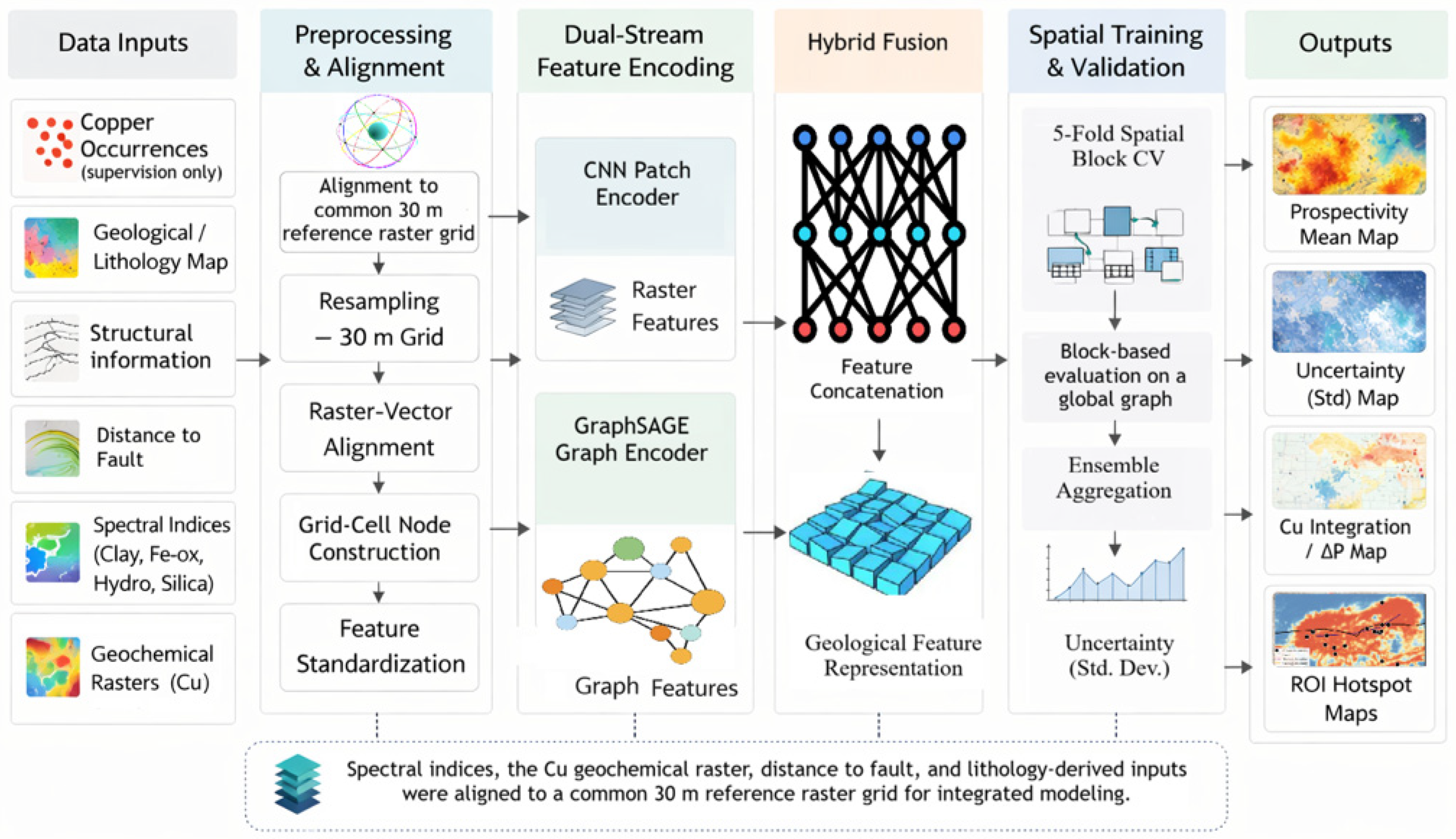
This study develops GeoHybridGNN as an implemented hybrid workflow for porphyry copper prospectivity mapping in the Western Chagai Belt. The workflow consists of six linked stages: input preparation, raster alignment to a common 30 m reference raster grid, graph node construction on regular grid cells, patch extraction and CNN-based raster encoding, hybrid GraphSAGE training on concatenated graph and raster-embedding features, and block-based spatial evaluation and map generation. After fold-wise training, predictions are aggregated to generate ensemble prospectivity products for exploration targeting. The final outputs include an ensemble mean prospectivity map, an uncertainty map expressed as the standard deviation across folds, probability difference maps for Cu geochemical integration, and ROI hotspot maps.

In the implemented workflow, raster information is represented through multi-channel patches extracted around node locations, whereas graph information is represented through node-level raster summaries, a lithology code, and regular grid adjacency. This design allows the model to combine continuous surface patterns with neighborhood-based spatial structure within one predictive system. Copper occurrence data were used only for supervised label assignment and evaluation and were not used as predictive inputs during inference. Accordingly, copper occurrences were excluded from predictive graph features, graph construction, and node attributes used for prediction. Figure 2 summarizes the overall implemented GeoHybridGNN workflow.

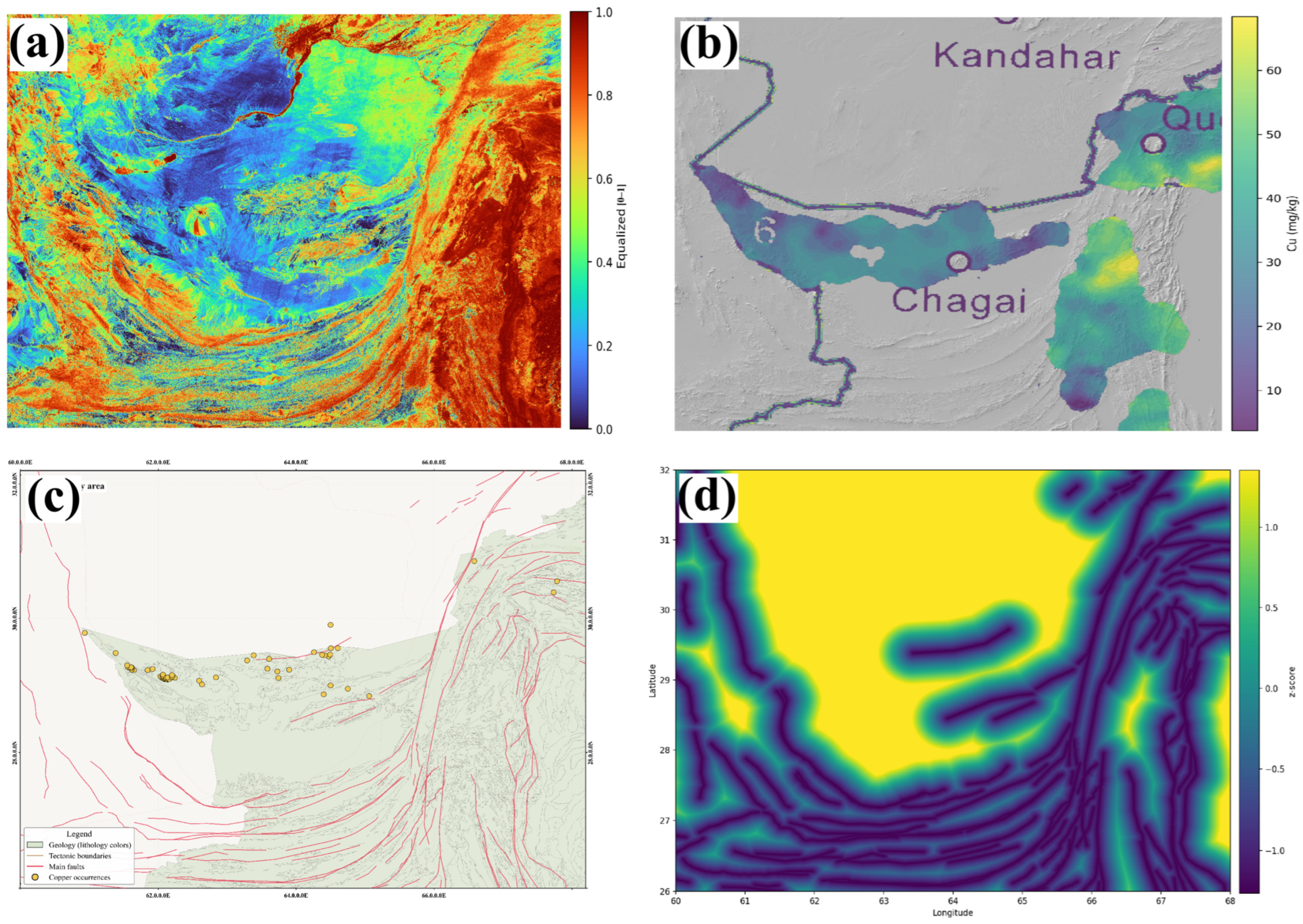
The implemented GeoHybridGNN workflow integrates aligned geoscientific raster layers that represent key controls on porphyry copper mineralization in the Western Chagai Belt. The principal continuous predictors include remote sensing-derived spectral alteration indices generated from harmonized Sentinel-2 surface reflectance imagery, the Cu geochemical raster, and the distance-to-fault raster. Lithology is incorporated separately as a categorical layer by rasterization to the common reference grid and subsequent coding as integer classes. Thus, geological and structural information enters the workflow through aligned raster predictors, node-level summaries, and patch extraction, while graph connectivity itself is defined by regular neighborhood relations on retained grid cells rather than by explicit fault-topology or tectonic-boundary topology.

The spectral inputs comprised remote sensing-derived clay-, iron-oxide-, hydrothermal-, and silica-related predictors generated from Sentinel-2 Surface Reflectance Harmonized imagery over the study area (26–32°N, 60–68°E). Sentinel-2 images acquired between 1 January 2023 and 31 December 2025 were filtered by cloud cover and processed using the Scene Classification Layer (SCL) to mask cloud shadow, medium- and high-probability cloud, cirrus, and snow pixels. A median composite was then generated over the ROI.

From this composite, the spectral alteration predictors used in GeoHybridGNN were calculated as follows: clay index $\mathrm{B}11/\mathrm{B}12$, iron-oxide index $\left(B4-B2)/(B4+B2\right)$, study-specific hydrothermal alteration proxy $B4/B2+B6/B11+B11/B12$, and silica index $B11/B4$. The hydrothermal alteration proxy was used as an operational composite rather than as a universally standardized porphyry copper index; it combines visible-band iron-sensitive contrast, red-edge to SWIR contrast, and SWIR clay/alteration-sensitive contrast, which are suitable for the arid Western Chagai Belt where vegetation cover is sparse and bedrock exposure is relatively good [28].

These remote sensing layers were exported as GeoTIFFs in EPSG:4326 at 30 m resolution and then reprojected and aligned to the common study reference raster grid. Before model construction, continuous rasters were resampled bilinearly, categorical rasters by nearest neighbor, and continuous predictors were subsequently standardized to z-scores and clipped to the interval $\left[-6, 6\right]$, whereas hillshade and lithology were excluded from continuous normalization. The Cu geochemical raster represented mineralization-related enrichment, and the distance-to-fault raster captured proximity to major structural corridors. The Cu geochemical raster was derived from the NGSSCA stream-sediment geochemical dataset of [35] Hong et al., which includes 9237 stream-sediment samples with an average density of approximately 1 sample per 100 km² across South and Central Asia.

In contrast, the copper occurrence dataset was reserved exclusively for label assignment, supervised training, and evaluation, and was not used as a predictive feature in either the raster branch or the graph branch. This distinction is important for preventing target leakage, particularly under spatial block cross-validation. Figure 3 shows the final input data layers used in GeoHybridGNN, and

Table 1. GeoHybridGNN input predictors, remote sensing data source, and spatial preparation for integrated modeling.

Predictor	Input Form	Final Spatial Form	Preparation for Modeling
Sentinel-2 spectral alteration stack	Sentinel-2 SR Harmonized multispectral image collection	30 m aligned raster layers	Remote sensing predictors were derived from harmonized Sentinel-2 surface reflectance imagery for the study area (26–32°N, 60–68°E) using images acquired from 1 January 2023 to 31 December 2025. Cloud- and shadow-contaminated pixels were masked using the Scene Classification Layer (SCL) by excluding classes 3, 8, 9, 10, and 11. A median composite was then generated over the ROI. The final spectral alteration stack used in GeoHybridGNN comprised clay $\left(B11/B12\right)$, iron oxide $\left((B4-B2)/(B4+B2)\right)$, a study-specific hydrothermal alteration proxy $\left(B4/B2+B6/B11+B11/B12\right)$, and silica $\left(B11/B4\right)$ indices. These rasters were exported as GeoTIFFs in EPSG:4326 at 30 m resolution, aligned to the common reference grid, z-score normalized, and clipped to $\left[-6, 6\right]$
Cu geochemical raster	NGSSCA stream-sediment Cu geochemical map/data [35]	30 m aligned raster layer	The Cu geochemical raster was derived from the NGSSCA stream-sediment Cu geochemical dataset. It was georeferenced/digitized, clipped to the study area, resampled to the 30 m reference grid, normalized, and used as the Cu geochemical predictor.
Lithology	Polygon vector	Rasterized categorical layer + node code	Lithology polygons were rasterized using the Name field, converted to integer codes, and aligned to the common reference grid. The value 0 was reserved for no data.
Distance to fault	Fault vector	30 m continuous raster	Faults were rasterized on the reference grid, and distance to the nearest fault pixel was computed.
Copper occurrences	Point vector	Supervision only	Used only for label assignment and evaluation, not as a predictive input.

summarizes the predictors and their spatial preparation for integrated modeling.

3.2. Spatial Preprocessing and Graph Construction

Before model construction, all raster predictors were aligned to a common 30 m reference raster grid. The preprocessing workflow reprojected and resampled all rasters to a shared study template and wrote aligned copies to the processed raster directory. Continuous rasters were resampled bilinearly, whereas categorical rasters were resampled by nearest neighbor. Lithology was rasterized to the same reference grid using the Name field and encoded as integer classes, with 0 reserved for nodata. The distance-to-fault raster was generated by rasterizing the fault layer on the same grid and computing the distance to the nearest fault pixel. Continuous raster predictors were then standardized to z-scores and clipped to the interval [−6, 6], whereas hillshade and lithology were excluded from continuous normalization. Quality-control scripts were also used to verify raster inventory, coordinate reference systems, vector clipping, raster alignment, and feature-to-reference consistency before model training.

Copper occurrence locations were converted from spreadsheet coordinates to point geometries, reprojected to the study reference system, clipped to the analysis extent, and then used only for supervised label assignment and evaluation. Background samples were generated within valid raster cells of the study extent, with an exclusion distance of 1000 m from known copper points, before raster predictors were sampled to build the supervised training table. After preprocessing, the study area was converted into a grid-cell graph using an explicit node and edge construction rule. Nodes were generated by partitioning the aligned reference raster grid into regular cells with a stride of 60 pixels. Because the grid spacing is 30 m, each node represents an area of approximately $1.8\times 1.8$ km. A node was retained only when the fraction of valid pixels within that cell was at least 0.20. For each retained cell, the graph builder stored the node identifier, geographic coordinates, the modal lithology code within the cell, and the mean value of each selected continuous raster predictor within the same cell. Thus, the node attributes consisted of the aligned continuous predictors described in Section 3.1, together with one categorical lithology code. Continuous node features were standardized globally using the mean and standard deviation computed across retained nodes, and non-finite values were replaced by zero before model training. Lithology was represented as an integer categorical code rather than as a one-hot vector. Graph adjacency was defined by a regular grid neighborhood structure rather than by explicit geological topology. Accordingly, lithological and structural controls are represented at a regional screening level in this study. Lithology is encoded as a categorical raster-derived node attribute, while structural information is represented mainly through distance-to-fault and related raster summaries. This simplified representation does not explicitly encode fault orientation, fault hierarchy, cross-cutting relationships, lithological contacts, alteration zonation, or tectonic-topology edges.

In the default configuration, each node was connected bidirectionally to its right and lower neighboring cells, which produced a 4-neighbor graph on the retained grid. Diagonal connections were added only when 8-neighborhood construction was explicitly requested. During model training, the adjacency matrix was symmetrized, self-loops were added, and row-normalized sparse aggregation was used for message passing. Therefore, the implemented graph encodes local spatial neighborhood continuity on the aligned grid, whereas lithological and structural information enters the model primarily through the node attributes and raster patches rather than through fault-topology or tectonic-boundary topology. Positive labels were assigned from the copper occurrence dataset only for supervised learning. First, a point-level training table was constructed by sampling aligned rasters at known copper points. $\left(label=1\right)$ and at 10,000 randomly generated background points $\left(label=0\right)$. Background points were sampled within the reference raster extent, restricted to valid raster cells, and filtered so that each retained background point lay at least 1000 m from any copper point. Second, positive graph nodes were created by assigning each positive copper point to its nearest graph node. To avoid unstable assignments, only point-to-node matches within $0.75$ times the median nearest-neighbor spacing of the node grid were retained.

Table 2. Summary of copper occurrence matching and positive graph node distribution across spatial folds.

Quantity	Value
Copper occurrence records used	90
Total graph nodes	184,140
Retained positive graph nodes	56
Fold 0 positive nodes	4
Fold 1 positive nodes	13
Fold 2 positive nodes	24
Fold 3 positive nodes	12
Fold 4 positive nodes	3

summarizes the copper occurrence records used for label assignment, the retained positive graph nodes after nearest-node matching, and their distribution across the five spatial folds.

In total, 90 copper occurrence records were used for label assignment. After applying the 0.75× median nearest-neighbor spacing rule, 56 positive graph nodes were retained. The retained positive nodes were distributed across the five spatial folds as follows: Fold 0 = 4, Fold 1 = 13, Fold 2 = 24, Fold 3 = 12, and Fold 4 = 3. Nodes receiving such an assignment were labeled positive, and all remaining nodes were treated as negative. Copper occurrences were therefore used only for label assignment and evaluation and were not used as predictive graph inputs.

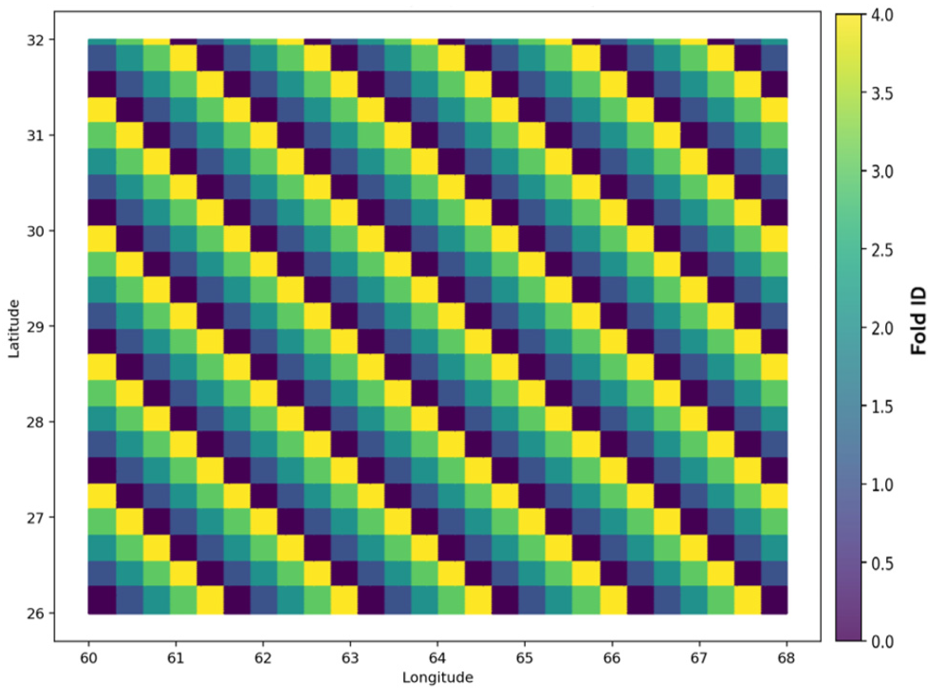
For spatial evaluation, five-fold spatial block cross-validation was defined on node coordinates using 30 km spatial blocks. One fold was used as the test fold, the next fold was used as the validation fold, and the remaining folds were used for training. In the present implementation, however, graph connectivity was constructed on the full node graph and was not rebuilt separately within each fold. The reported validation design should therefore be interpreted as block-based evaluation on a global graph rather than as fold-isolated message passing. This setting is transductive because the graph structure is constructed once over all retained nodes. Although labels from validation and test folds are not used for training, message passing can still occur across edges connecting nodes from different spatial folds. Therefore, the reported AUC values may be more optimistic than those from a fully inductive setting in which each fold is represented by an independently reconstructed or edge-isolated graph. The magnitude of this effect cannot be quantified exactly without running a separate fold-isolated graph experiment, but it is expected to affect mainly nodes close to spatial-fold boundaries where cross-fold edges permit neighborhood aggregation. For this reason, the reported AUC values are used as transductive block-based performance estimates and should be interpreted cautiously rather than as fully independent generalization scores.

3.3. Dual-Stream Encoding and Concatenation-Based Hybrid Fusion

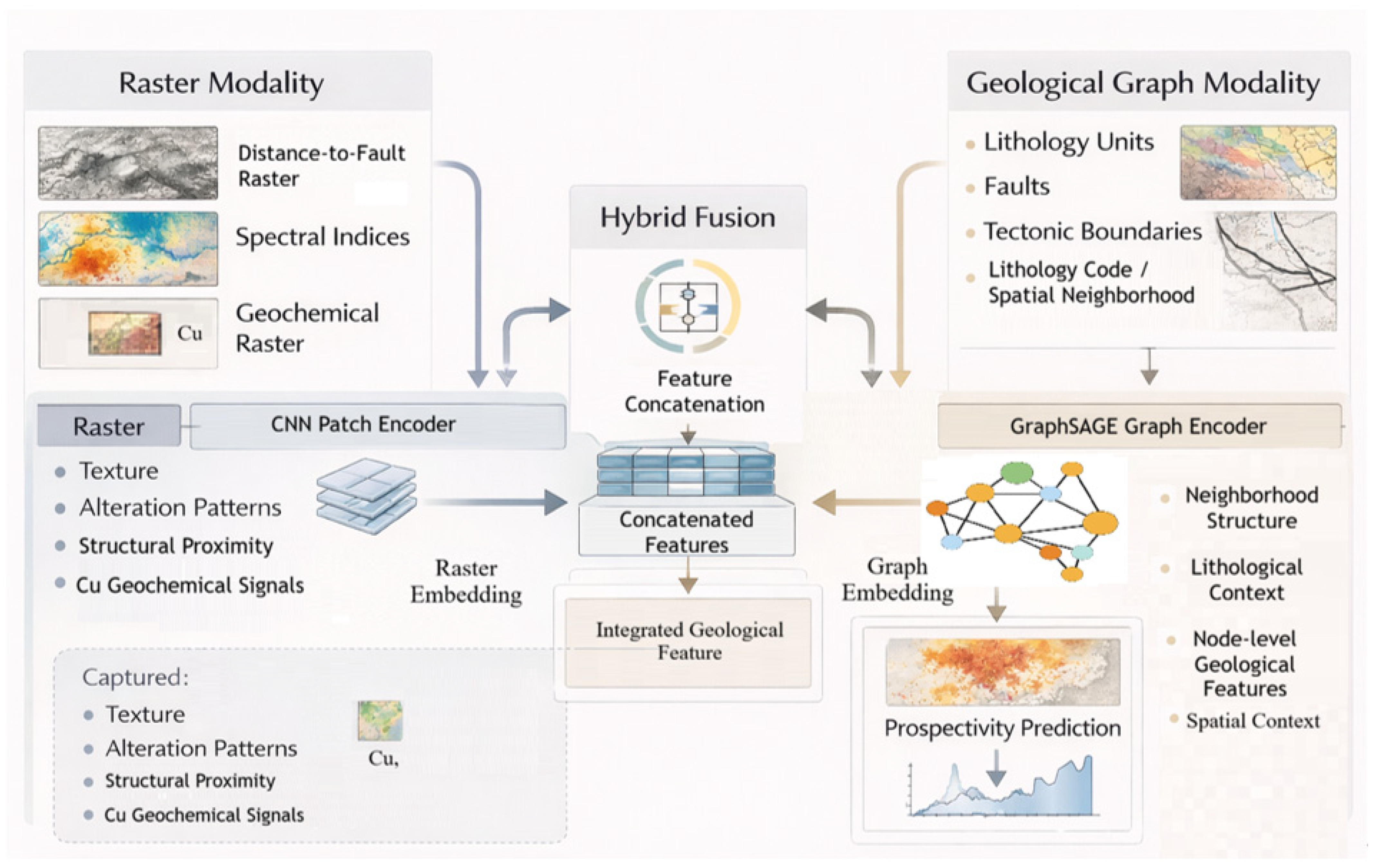
A central feature of the implemented framework is its dual-stream design, in which raster and graph information are processed separately before hybrid prediction. This design is important because the two data types have different spatial structures and therefore require different forms of representation learning. Raster data preserve continuous spatial variation across the study area, whereas graph data preserve neighborhood relations among retained grid cells. In the present implementation, the regular 4-neighbor graph is not intended to represent explicit fault connectivity or geological topology. Its purpose is to support node-level aggregation of geological and raster-derived summaries across retained grid cells. This is different from the CNN branch, which learns local texture and spectral patterns from raster patches. Therefore, the GraphSAGE branch complements the CNN branch by operating on lithology-coded node attributes, distance-to-fault summaries, spectral-index summaries, and CNN-derived embeddings within a neighborhood-propagation framework. Processing them in separate branches allows the model to learn complementary features from each modality before integration. The raster branch uses a CNN patch encoder rather than a transformer. Multi-channel raster patches of size $32\times 32$ pixels were extracted around training points and graph node locations from the aligned raster stack. Patches intersecting the raster boundary were excluded, and patches with more than 20% nodata were also discarded. For retained patches, remaining nodata values were replaced by 0 after normalization.

The CNN encoder consists of three convolutional blocks with 32, 64, and 128 channels, respectively. Max-pooling is applied after the first and second convolutional blocks, and adaptive average pooling is applied after the third block. The pooled representation is then projected through a fully connected layer to a 64-dimensional embedding with ReLU activation and dropout. During patch-level training, a single linear output head is used for binary classification; after training, the learned 64-dimensional embedding is exported for each graph node and used as the raster component of the hybrid model. These 64-dimensional embeddings are latent representations of the multi-channel raster patches and should not be interpreted as one-to-one physical geological variables. Their geological relevance comes from the input channels used to generate them, including spectral alteration predictors, distance-to-fault information, Cu geochemistry where included, lithology-related raster information, and other aligned geoscientific layers. The raster input channels correspond to the aligned normalized predictor layers selected for the experiment, excluding hillshade and optionally including lithology as an additional channel. The graph branch uses a GraphSAGE-based graph encoder implemented as a full-batch GraphSAGE model. The graph is built on retained grid cells, and each node carries the modal lithology code together with the mean values of the selected continuous raster predictors extracted at the node-cell scale.

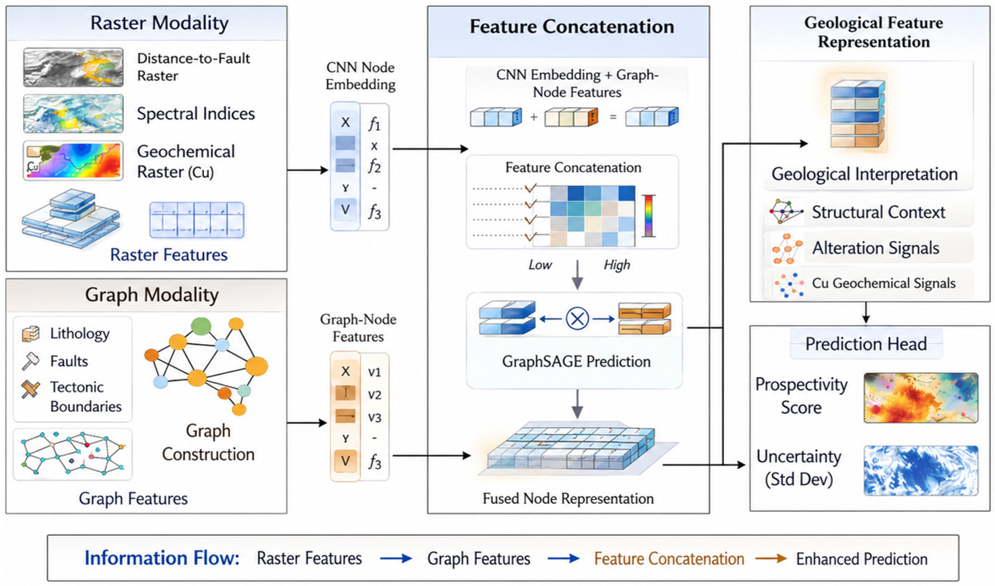
After the raster embeddings are exported, the 64-dimensional CNN embedding for each node is concatenated with the normalized node-feature vector to form the hybrid input representation. The graph encoder then applies two GraphSAGE layers with hidden dimension 64, ReLU activation, and dropout 0.2, followed by a linear prediction head that outputs one logit per node. During message passing, the adjacency matrix is symmetrized, self-loops are added, and row-normalized sparse aggregation is used. Therefore, the implemented fusion mechanism is based on feature concatenation followed by GraphSAGE-based graph aggregation, rather than on an attention-based fusion block. In this way, the raster branch emphasizes continuous surface patterns learned from local patches, whereas the graph branch emphasizes neighborhood continuity and node-level geological context on the retained grid. Figure 4 illustrates the overall implemented GeoHybridGNN architecture, including the CNN patch encoder, the GraphSAGE graph encoder, concatenation-based hybrid fusion, and the final prediction head. The fusion sub-step is shown separately in Figure 5. In the implemented workflow, the 64-dimensional CNN node embeddings are concatenated with the normalized graph node features before GraphSAGE-based prediction.

3.4. Spatial Validation and Output Generation

Model training and evaluation were performed using five-fold spatial block cross-validation defined on graph nodes. Node coordinates were converted approximately to kilometers using the median latitude of the study area, and block indices were obtained by dividing the spatial coordinates by a block size of 30 km. The fold assignment was then defined deterministically from the spatial block identifier modulo 5. In each run, one fold was used as the held-out test fold, the next fold $(\mathrm{t}\mathrm{e}\mathrm{s}\mathrm{t}\text{\_}\mathrm{f}\mathrm{o}\mathrm{l}\mathrm{d}+1) mod 5$ was used as the validation fold, and the remaining folds were used for training. Thus, the node-based evaluation was approximately 60% training, 20% validation, and 20% testing in each run, subject to the spatial distribution of retained nodes. In the present implementation, graph connectivity was constructed on the full node graph and was not rebuilt separately within each fold. The reported validation scheme should therefore be interpreted as block-based evaluation on a global graph rather than as fully fold-isolated message passing. Even with this limitation, the blocked partition provides a more spatially realistic assessment than ordinary random splitting at the label-evaluation level. However, because graph connectivity remains global, the results should be interpreted as transductive block-based evaluation rather than fully inductive graph generalization. Figure 6 shows the spatial block cross-validation design used in this study. The raster patch encoder was trained first on the extracted patch dataset. Patch-level training used a stratified random split with approximately 70% of samples for training, 15% for validation, and 15% for testing.

The CNN encoder was optimized with weighted binary cross-entropy with logits using AdamW, learning rate ${10}^{-3}$, weight decay ${10}^{-4}$, batch size 128, and a maximum of 25 epochs. To reduce class imbalance, the training loader used a weighted random sampler, and the positive-class loss weight was set to $n_{\mathrm{n}\mathrm{e}\mathrm{g}}/n_{\mathrm{p}\mathrm{o}\mathrm{s}}$ within the training subset. The best checkpoint was selected by minimum validation loss and then applied to all graph nodes to export 64-dimensional raster embeddings. In the preprocessing and split-generation scripts, a fixed seed of 7 was used where stochastic sampling or splitting was required. The hybrid graph model was then trained in full-batch mode using the concatenated node-feature vector and the 64-dimensional CNN embedding for each node. The graph classifier used weighted binary cross-entropy with logits, AdamW optimization, learning rate ${10}^{-3}$, weight decay ${10}^{-4}$, two GraphSAGE layers, hidden dimension 64, and dropout 0.2. Training was run for a maximum of 30 epochs, and early stopping was monitored by validation loss with patience 5. To address class imbalance, the positive-class loss weight was computed from the training fold as $n_{\mathrm{n}\mathrm{e}\mathrm{g}}/n_{\mathrm{p}\mathrm{o}\mathrm{s}}$ and clipped at 500 when necessary. Gradient clipping with maximum norm 1.0 was also applied during optimization.

Final test performance was summarized using ROC-AUC, average precision, log loss, and Brier score. After the five-fold runs were completed, predictions were aggregated to produce the final ensemble outputs, including the ensemble mean prospectivity map, the uncertainty map expressed as the standard deviation across folds, probability difference maps for Cu geochemical integration, and ROI hotspot maps for focused interpretation of key target zones. Model performance was summarized using ROC curves and precision-recall curves. Together with the uncertainty and ablation maps, these outputs provide a more informative assessment of GeoHybridGNN than any single summary score alone. The core configuration and evaluation settings of the implemented GeoHybridGNN workflow are summarized in

Table 3. Core configuration and evaluation settings of the implemented GeoHybridGNN.

Component	Setting
Reference raster grid	30 m
Graph node stride	60 pixels
Node footprint	~1.8 × 1.8 km
Node retention threshold	Valid-pixel fraction ≥ 0.20
Raster patch size	32 × 32 pixels
CNN encoder channels	32/64/128
CNN embedding size	64
Graph model	2-layer GraphSAGE
Graph hidden dimension	64
Fusion	Feature concatenation
Dropout	0.2
Optimizer/loss	AdamW/weighted BCE with logits
Learning rate/weight decay	$1\times {10}^{-3}/1\times {10}^{-4}$
Training length	25 epochs (CNN), 30 epochs (GNN)
Early stopping	Patience = 5
Spatial validation	5-fold spatial block CV, 30 km blocks
Graph evaluation mode	Global graph with block-based label evaluation

.

4. Results

4.1. Spatial Validation Performance

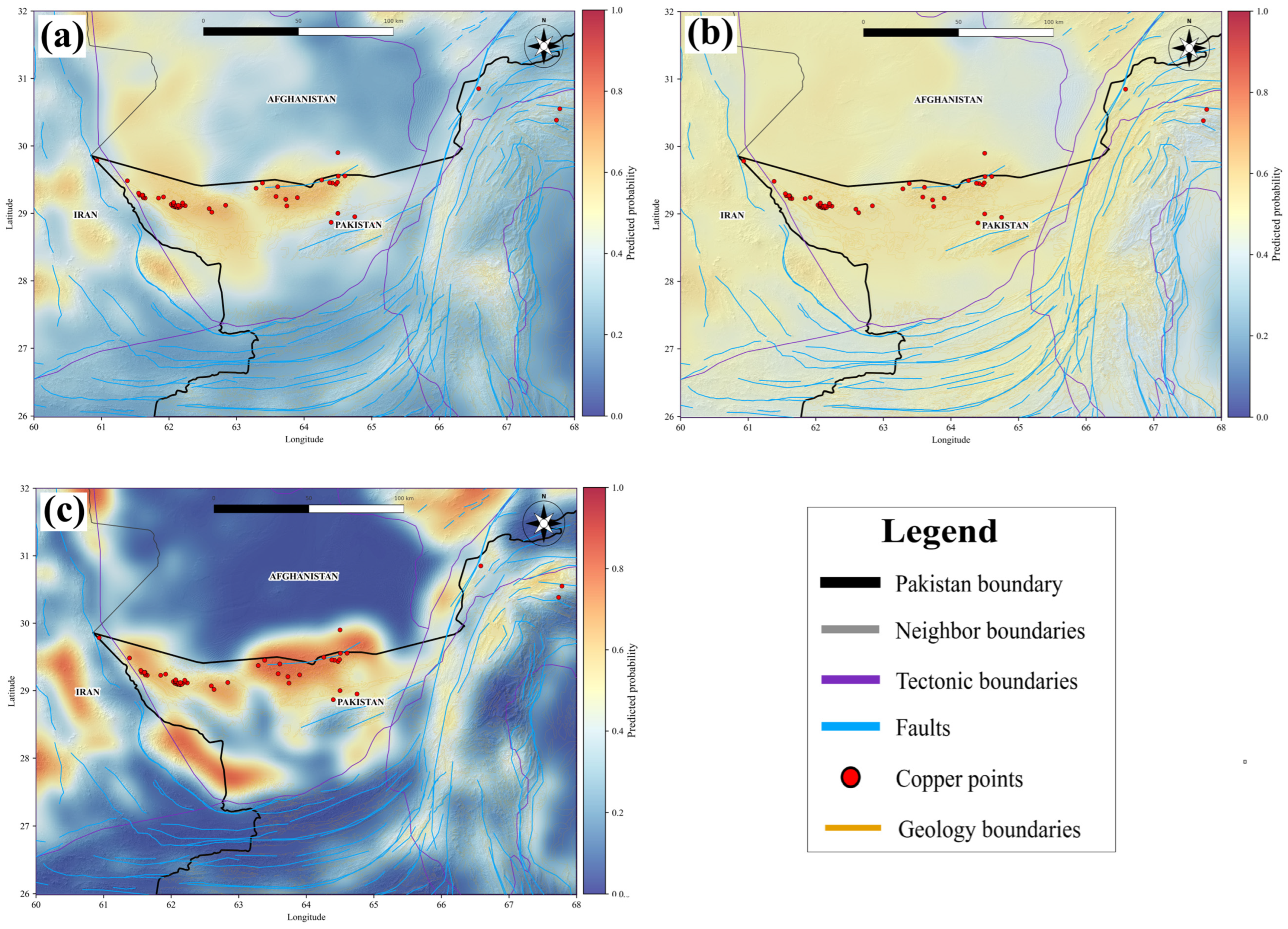
The results show that GeoHybridGNN performs well under the adopted block-based validation design and produces prospectivity maps that are geologically interpretable and spatially coherent. Across the full workflow, three main patterns are evident. First, the hybrid model remains robust under 5-fold spatial block cross-validation. Second, the final prospectivity maps are more coherent than those of the comparison models. Third, adding the Cu geochemical raster changes the global score only slightly, but provides modest local target sharpening in selected zones, as further quantified by the top-ranked-area hit-rate analysis in Section 4.5. The fold-wise quantitative results suggest that the hybrid model is reasonably stable under the adopted blocked validation design.

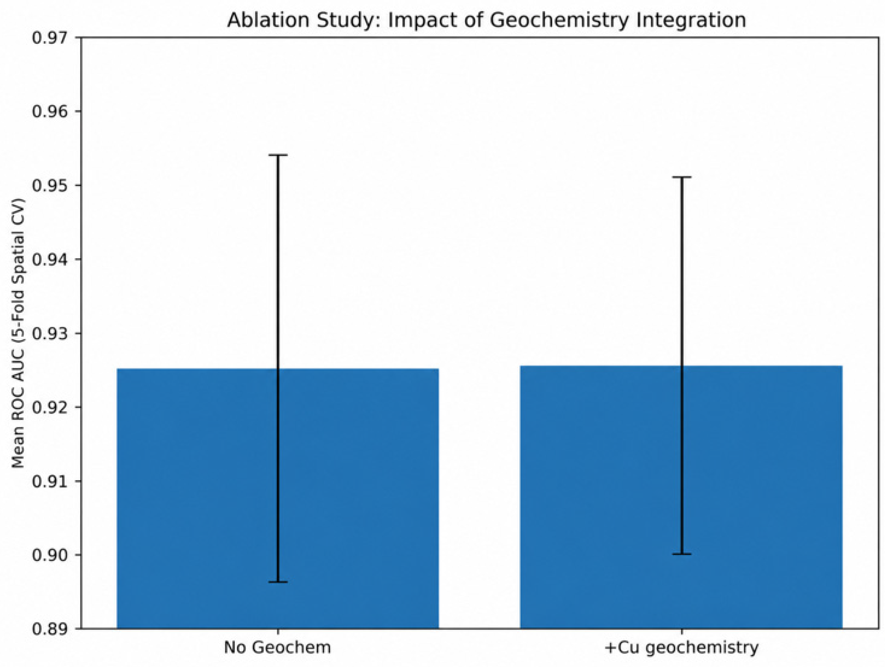
The ablation analysis shows that the mean ROC AUC changes only from 0.9252 to 0.9256 after adding the Cu geochemical raster. This indicates that the large-scale predictive structure is captured mainly by geological and structural information, while Cu geochemistry acts primarily as a local refinement factor rather than the main driver of regional performance. The results also show stable behavior across the five folds. In the comparative metric panel, GeoHybridGNN achieves the highest mean ROC AUC among the tested models, with GAT and GraphSAGE showing lower ROC-AUC values under the updated comparison. Figure 7 summarizes the fold-wise spatial block cross-validation performance and the effect of Cu geochemical integration on model accuracy. The fold-wise spatial block cross-validation results for GeoHybridGNN with and without Cu geochemical integration are summarized in

Table 4. Fold-wise spatial block cross-validation performance of GeoHybridGNN with and without Cu geochemical integration.

Model	Fold0	Fold1	Fold2	Fold3	Fold4	Mean AUC	Std
Hybrid (No Geochem)	0.9360	0.8935	0.9650	0.8903	0.9411	0.9252	0.0289
Hybrid (+Cu–geochemistry)	0.9330	0.8945	0.9697	0.9090	0.9217	0.9256	0.0255

.

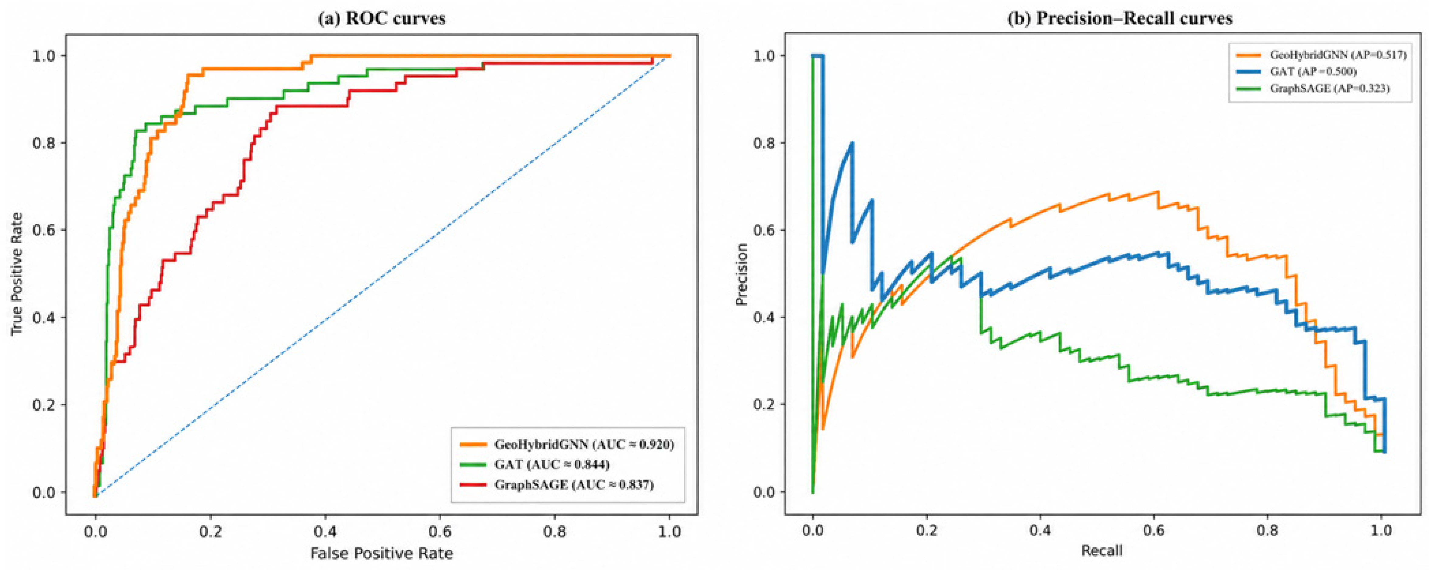
The ranking observed in the model comparison is further supported by the ROC and precision-recall analysis. In the ROC curves, GeoHybridGNN achieves the highest AUC, about 0.920, compared with 0.844 for GAT and 0.837 for GraphSAGE. This suggests that the hybrid integration of raster and graph features improves overall discrimination between favorable and unfavorable locations under the adopted evaluation setting. The precision-recall curves provide a complementary view of predictive performance under class imbalance, which is important in exploration settings. Overall, GeoHybridGNN shows the strongest precision-recall tradeoff among the compared models, with AP = 0.517 compared with 0.500 for GAT and 0.323 for GraphSAGE, indicating that it is not only accurate in a global sense but also effective in concentrating known mineralization within the most prospective parts of the map. Figure 8 presents the ROC and precision-recall curves used for this comparison.

Table 5. Fold-wise AUC comparison between GeoHybridGNN and GAT with paired Wilcoxon test result.

Model	Fold 0	Fold 1	Fold 2	Fold 3	Fold 4	Mean AUC	Std
GeoHybridGNN	0.9255	0.9183	0.9241	0.9205	0.9115	0.9200	0.0055
GAT	0.7737	0.8420	0.7498	0.9229	0.9326	0.8442	0.0835

Note: The paired Wilcoxon signed-rank test between GeoHybridGNN and GAT gave statistic = 3.0 and p = 0.3125.

summarizes the fold-wise AUC values for GeoHybridGNN and GAT and reports the paired Wilcoxon signed-rank test used to assess the statistical support for their AUC difference. To further assess whether the AUC difference between GeoHybridGNN and GAT was statistically supported across folds, we performed a paired Wilcoxon signed-rank test using the five fold-wise AUC values. The result was not statistically significant at the 0.05 level (statistic = 3.0, p = 0.3125). Therefore, the AUC advantage of GeoHybridGNN over GAT is interpreted cautiously. GeoHybridGNN achieved the higher mean fold-wise AUC and lower fold-wise variability, but its practical advantage is discussed together with the clearer spatial coherence and uncertainty organization of the resulting maps.

4.2. Uncertainty Patterns and Spatial Generalization

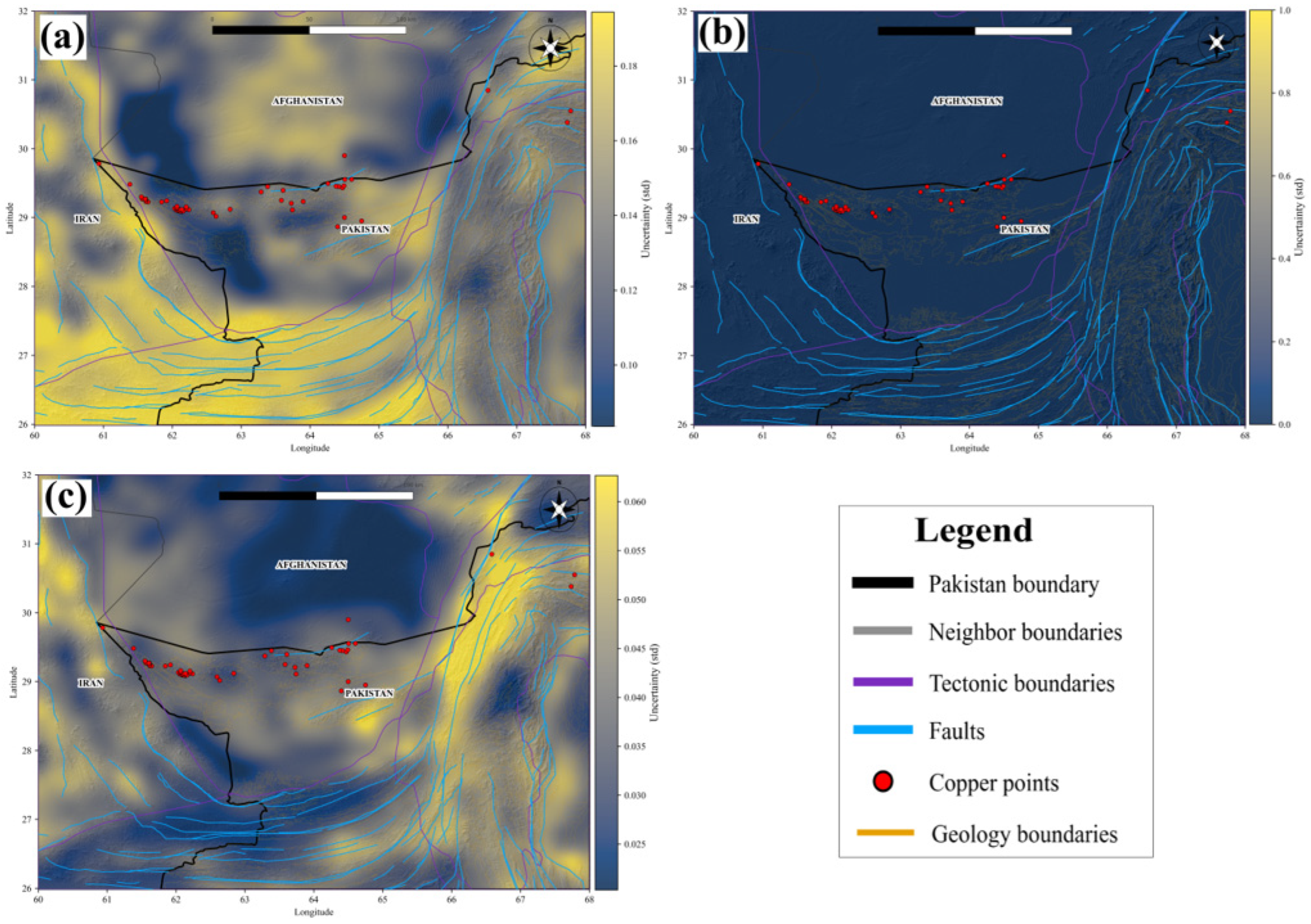
The uncertainty maps provide an additional diagnostic layer by showing where fold-wise predictions remain stable and where they are more sensitive under spatial block cross-validation. In this study, uncertainty is represented by the standard deviation of ensemble predictions across folds, and therefore it should be interpreted as a fold-wise prediction-stability indicator rather than as a fully calibrated geological uncertainty map. Low standard deviation indicates agreement among fold-specific predictions, but it does not automatically imply geological certainty, because low variance may also occur in uniformly low-prospectivity areas or in sparsely sampled regions where the model consistently assigns low scores. For this reason, the uncertainty maps were interpreted together with the ensemble mean prospectivity map, known copper occurrences, structural corridors, and geological context. GeoHybridGNN produces more spatially coherent uncertainty patterns than the comparison models, and these patterns broadly follow the main structurally controlled prospective corridor of the Western Chagai Belt.

However, this result is interpreted as improved prediction stability and spatial organization under the adopted block-based evaluation, not as direct proof of geological certainty. GAT and GraphSAGE also capture parts of the broad uncertainty structure, but GeoHybridGNN shows a clearer correspondence between stable prediction zones and the main prospective trend. Figure 9 presents the prediction-stability maps for the three graph-based models and highlights the clearer spatial organization achieved by GeoHybridGNN. From an exploration perspective, these uncertainty maps are useful because they complement the prospectivity scores themselves: high-prospectivity areas with stable fold-wise predictions can be prioritized more confidently, whereas high-score areas with larger fold-wise variability should be treated more cautiously. At the same time, low-uncertainty areas far from known copper occurrences should not be interpreted as confirmed low-risk geological zones unless supported by the mean prospectivity map and geological evidence. Thus, the uncertainty maps strengthen the practical value of the workflow by supporting cautious, spatially informed prioritization of follow-up targets, while remaining an auxiliary stability indicator rather than a stand-alone measure of geological risk.

To further check whether the uncertainty layer reflects useful prediction-stability information, we compared the GeoHybridGNN uncertainty map with prediction error and distance to retained positive copper nodes, as summarized in

Table 6. Diagnostic checks for the GeoHybridGNN uncertainty map.

Diagnostic Check	Result	Interpretation
Uncertainty vs. absolute prediction error	Spearman ρ = 0.604, p < 0.001	Higher fold-wise variability is associated with larger prediction error.
Uncertainty vs. distance to nearest retained positive node	Spearman ρ = −0.081	Uncertainty is not simply controlled by distance from known copper nodes.
Low-uncertainty far-zone check	Mean prospectivity = 0.067; retained positives = 0	Low variance in sparse/far areas mainly reflects stable low-prospectivity predictions, not geological certainty.

Note: Diagnostics were computed using the GeoHybridGNN with-Cu ensemble mean and standard-deviation maps and the 56 retained positive graph nodes.

.

4.3. Final Prospectivity Patterns and Target Zones

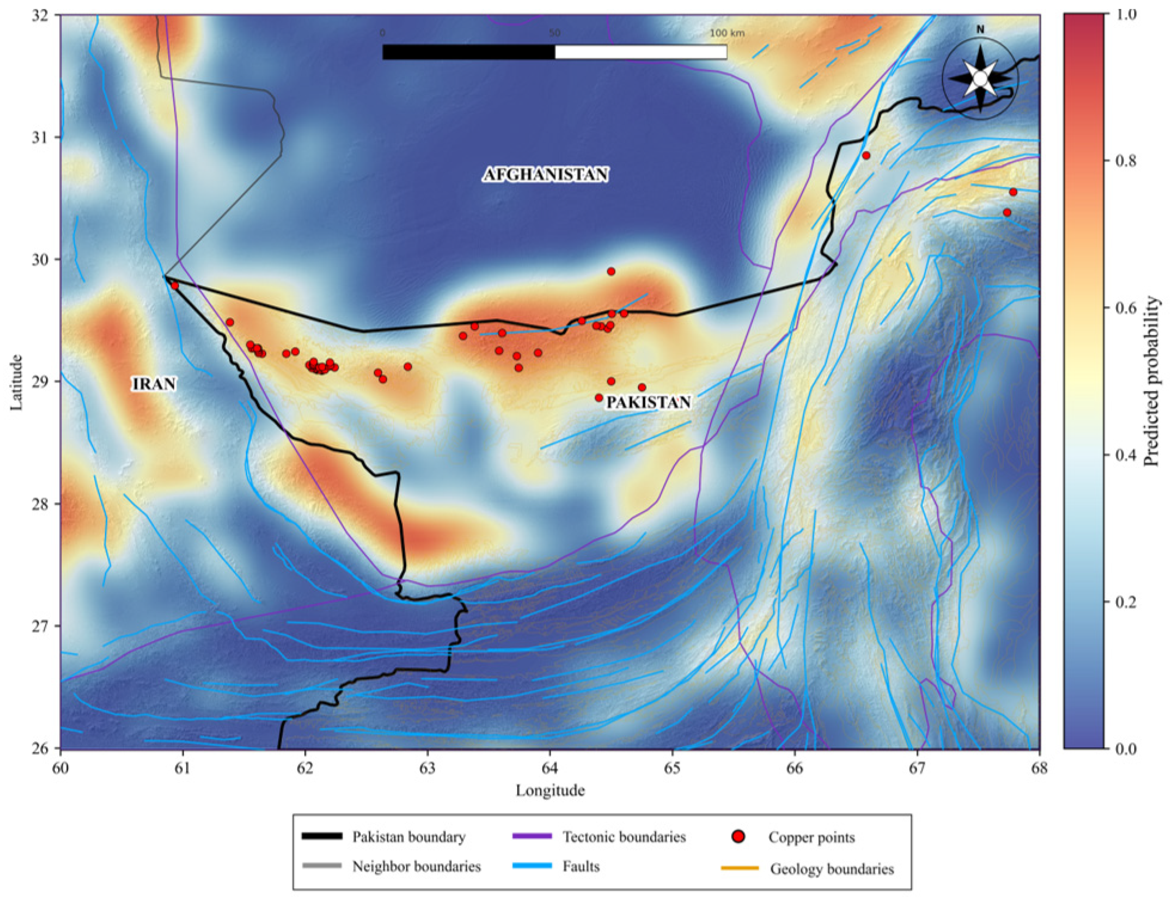
The final ensemble mean prospectivity map shows a strong and geologically reasonable concentration of high scores within the main mineralized corridor of the Western Chagai Belt. These results highlight spatial hotspots, structural control, alignment with known copper occurrences, and consistency with the regional metallogenic framework. GeoHybridGNN identifies a central east-to-west and northeast to southwest prospective belt that closely follows the main mineralized trend. The anomaly pattern is neither overly diffuse nor overly fragmented. Instead, it forms connected target zones that are easier to interpret in geological terms. Figure 10 presents the final ensemble mean prospectivity map produced by GeoHybridGNN and highlights the principal prospective corridor and major target zones. This result is important because the final map does more than identify isolated high-score pixels. It preserves the broader structural continuity of the mineralized belt while also distinguishing internally focused target zones that are more useful for exploration follow-up. In this sense, the final ensemble output provides both regional geological consistency and local targeting value. The ROI panels further show that this pattern is not restricted to a single location. Similar behavior appears in multiple target sectors, including Chagai Core, Central Belt, East Corridor, and South Center Corridor, indicating that the model captures both the main prospective belt and its local internal variation.

4.4. Model Comparison

A direct visual comparison of the three graph-based models helps clarify the differences in performance. Although all three models identify the main mineralized corridor, they differ in how clearly and coherently they represent its internal structure. The GAT map captures the same broad favorable zone, but its response is somewhat more diffuse in several areas. GraphSAGE also reproduces the general corridor, but the anomaly field is smoother and less sharply focused, which reduces local target definition. In contrast, GeoHybridGNN provides the most balanced output by preserving the large-scale structural pattern while also sharpening the central hotspot belt and related target zones. Figure 11 compares the ensemble mean prospectivity maps of GAT, GraphSAGE, and GeoHybridGNN and highlights the stronger spatial coherence achieved by the proposed framework. To further isolate the contribution of the raster and graph branches, we added an ablation comparison including a raster-only CNN patch encoder, a graph-only GraphSAGE model, and the final hybrid GeoHybridGNN model. These baselines were selected because they directly correspond to the implemented components of the proposed architecture: the CNN branch represents raster-patch learning, the graph-only GraphSAGE model represents neighborhood aggregation using node attributes and regular 4-neighbor adjacency, and GeoHybridGNN represents their hybrid concatenation-based integration. We did not include Random Forest or MLP baselines in this revision because they would require a separate tabular feature design and would not directly test the raster-patch and graph node components of the proposed workflow. The raster-only CNN result is reported as a patch-level branch diagnostic, whereas the graph-only GraphSAGE and GeoHybridGNN results are evaluated under the spatial block node-level protocol. The ablation results are summarized in

Table 7. Ablation comparison of raster-only, graph-only, and hybrid GeoHybridGNN components.

Model	Input Information	Evaluation Setting	AUC
Raster-only CNN patch encoder	Raster patches only	Stratified patch-level test split	0.9286
Graph-only GraphSAGE	Node attributes + 4-neighbor graph	5-fold spatial block node evaluation	0.8369 ± 0.0945
GeoHybridGNN	CNN embeddings + node attributes + 4-neighbor graph	5-fold spatial block node evaluation	0.9200 ± 0.0055

.

The ablation results show that the raster branch can learn useful patch-level information, while the graph-only GraphSAGE baseline is weaker under spatial block node-level evaluation. Adding CNN-derived raster embeddings to the graph node features increases the mean spatial-block AUC and reduces fold-wise variability relative to the graph-only baseline. Therefore, the results support the contribution of dual-modal fusion, although the improvement should be interpreted as the combined effect of raster patch encoding, node attributes, and neighborhood aggregation rather than as evidence that fusion alone is the only performance driver. Therefore, the comparison is intended to evaluate the contribution of the implemented raster and graph components rather than to provide an exhaustive benchmark against all possible machine-learning classifiers. Threshold-free AUC and AP were emphasized because the prospectivity map is used as a continuous ranking product, whereas threshold-dependent metrics such as F1-score depend on an additional cutoff choice.

This comparison is important because prospectivity mapping is not only about identifying broad favorable regions, but also about distinguishing target zones that are spatially meaningful and practical for follow-up exploration. In this respect, GeoHybridGNN shows a practical advantage in terms of spatial coherence and target organization, although the fold-wise AUC difference relative to GAT should be interpreted cautiously because the paired Wilcoxon test was not statistically significant. Its anomaly pattern is more continuous than that of GAT, yet more focused than that of GraphSAGE, which gives a better balance between regional continuity and local target discrimination. The resulting map is easier to interpret in geological terms because it aligns more clearly with the main structural corridor and known mineralization trend. Overall, the comparison suggests that the proposed GeoHybridGNN framework provides stronger predictive integration of the selected inputs than the tested comparison models. Rather than relying only on graph attention or a simpler graph-only aggregation strategy, GeoHybridGNN combines raster-derived structural information, lithology-coded node attributes, alteration-related raster signals, and Cu geochemical information within a single concatenated feature space. This likely explains why the proposed model gives the most spatially coherent and geologically focused performance under the selected validation design.

4.5. Effect of Cu Geochemical Integration and ROI Hotspot Analysis

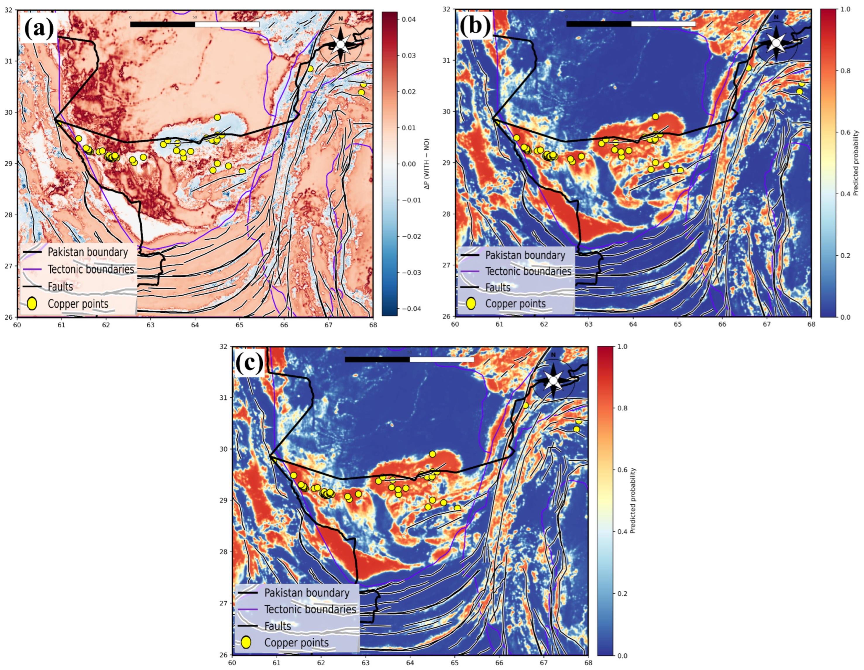
The Cu geochemical integration results provide an important view of the difference between global and local model behavior. As shown in Figure 12, positive DeltaP values highlight zones where Cu geochemistry enhances prospectivity prediction, whereas near-zero regions indicate stronger control by the geological and structural framework. Most of the study area shows only small changes, which is consistent with the limited change in global ROC AUC. To quantify this local effect, we additionally evaluated target-delineation metrics using the 56 retained positive graph nodes. The results are summarized in

Table 8. Local target-delineation metrics for Cu geochemical integration.

Model	Top 5% Hits	Top 5% Hit Rate	Top 10% Hits	Top 10% Hit Rate	Top 20% Hits	Top 20% Hit Rate
Hybrid without Cu geochemistry	29/56	51.8%	44/56	78.6%	54/56	96.4%
Hybrid with Cu geochemistry	30/56	53.6%	44/56	78.6%	54/56	96.4%

Note: Hit rates were computed using the 56 retained positive graph nodes after nearest-node matching. The top 5%, 10%, and 20% areas correspond to target-area reductions of 95%, 90%, and 80%, respectively.

. Cu geochemical integration increased the top-5% hit rate from 51.8% to 53.6%, corresponding to one additional retained positive node in the highest-ranked 5% prospectivity area, while the top-10% and top-20% hit rates remained unchanged. Therefore, the Cu layer is interpreted as providing modest local target sharpening rather than a substantial global discrimination gain. However, several localized corridors and patches show positive increases, reaching about +0.10 in the most enhanced zones, while a few limited negative patches indicate small local decreases. 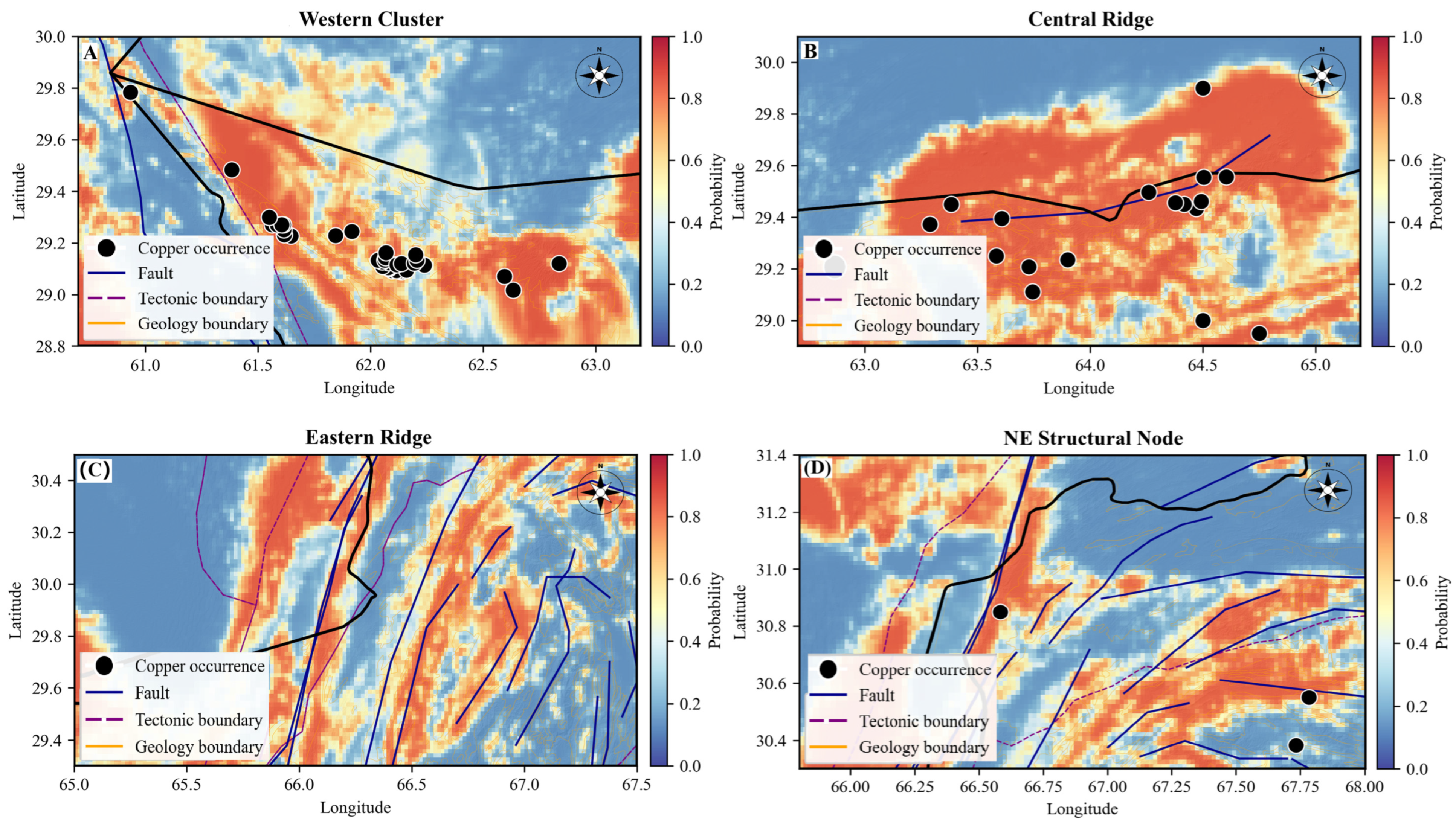The strongest positive DeltaP responses occur mainly within and near the principal mineralized corridor and the focused ROI sectors shown in Figure 13, including the Western Cluster, Central Ridge, Eastern Ridge, and NE Structural Node. These sharpened zones are therefore interpreted as local refinements around known mineralized centers and adjacent structurally favorable target areas, rather than as confirmed greenfield discoveries.

When the mean and uncertainty maps are compared for the settings with and without Cu geochemical integration, the main prospective architecture remains broadly the same, but the integrated model sharpens selected internal anomalies and slightly redistributes uncertainty in a few focused areas. This indicates that Cu geochemistry does not simply inflate the prospectivity map. Instead, it produces localized redistribution of prospectivity scores, while the structural and lithological framework continues to control the regional prospectivity pattern. To examine whether the Cu-driven contribution was directly coupled with structural or alteration predictors, we performed a node-level diagnostic using the DeltaP map, distance-to-fault values, and the hydrothermal alteration index. The coupling was weak: DeltaP showed only a weak association with distance to fault (Spearman $\rho =0.108$, $p<0.001$) and a weak negative association with the hydrothermal index (Spearman $\rho =-0.145$, $p<0.001$). The mean DeltaP in the combined near-fault and high-hydrothermal zone was 0.0057, compared with an overall mean DeltaP of 0.0110. These results indicate that the Cu contribution is not controlled by a simple pairwise coupling with fault proximity or alteration intensity. Therefore, Cu geochemistry is interpreted more cautiously as a context-dependent local refinement factor rather than as evidence of a direct mechanistic coupling with structural or alteration predictors.

The ROI hotspot maps provide a closer view of how the final GeoHybridGNN output behaves within the main target sectors. These panels show that the identified anomalies are not confined to one isolated area, but recur across several geologically meaningful zones within the Western Chagai Belt. In particular, the hotspot patterns remain aligned with the broader prospective corridor while also distinguishing more focused internal targets suitable for follow-up investigation. This is consistent with the interpretation that the final model captures both regional continuity and local target refinement under the adopted block-based evaluation design. Figure 13 presents the ROI hotspot maps for the main target sectors and further demonstrates the spatial concentration and geological consistency of the final prospectivity results. Overall, the results support three main conclusions.

First, GeoHybridGNN performs strongly and consistently under spatial block cross-validation. This indicates that the proposed workflow remains robust when evaluation is carried out under a more spatially realistic partitioning strategy rather than ordinary random splitting. Second, its prospectivity and uncertainty maps are more coherent and easier to interpret than those of the comparison models. In particular, the final outputs better preserve the main mineralized corridor while also distinguishing internally focused target zones that are more practical for follow-up exploration. Third, Cu geochemical integration provides modest local refinement in target definition, even though it does not substantially change the global discrimination score. This suggests that Cu geochemistry acts mainly as a local refinement factor that sharpens selected anomalies where it is spatially consistent with the broader geological and structural framework.

Together, these outputs provide a practical and geologically interpretable basis for porphyry copper targeting in the Western Chagai Belt. They also show that the proposed framework can support both regional prospectivity assessment and more focused exploration prioritization within the belt. To test whether the Cu-driven local refinement is directly coupled with structural or alteration evidence, we compared the node-level DeltaP values with distance-to-fault and hydrothermal alteration intensity. DeltaP represents the change in predicted prospectivity after adding the Cu geochemical raster. If Cu geochemistry were strongly coupled with structural or alteration controls, positive DeltaP values would be expected to increase systematically near faults or in high-alteration zones. The node-level coupling diagnostics are summarized in

Table 9. Node-level coupling diagnostics between Cu geochemical contribution and geological predictors.

Coupling Metric	Value	Interpretation
DeltaP vs. distance to fault	Spearman ρ = 0.108, p < 0.001	Weak pairwise association; no strong direct near-fault coupling.
DeltaP vs. hydrothermal alteration index	Spearman ρ = −0.145, p < 0.001	Weak negative association; no simple positive alteration coupling.
Mean DeltaP in near-fault + high-hydrothermal zone	0.0057 vs. overall mean 0.0110	Cu effect is localized and context-dependent, not controlled by this simple coupled condition.

Note: DeltaP represents the probability difference between the GeoHybridGNN outputs with and without Cu geochemical input. Coupling diagnostics were computed at graph node level using aligned node predictors.

.

The weak pairwise associations indicate that the Cu contribution is not controlled by a simple direct coupling with fault proximity or hydrothermal alteration intensity alone. Therefore, the Cu geochemical layer is interpreted more cautiously as a context-dependent local refinement factor, acting together with the broader lithological, structural, and raster-derived evidence rather than as an independent mechanistic control.

5. Discussion

The results show that GeoHybridGNN provides a strong balance between predictive performance, spatial coherence, and geological interpretability for porphyry copper prospectivity mapping in the Western Chagai Belt. The main advantage of the model is not only that it reaches high predictive scores, but that it does so under a block-based spatial validation design. This is important because mineral prospectivity models can appear strong under random splits but weaken when tested across spatially separated areas. In this study, 5-fold spatial block cross-validation provides a more spatially realistic assessment than ordinary random splitting, although the current graph implementation should be interpreted as block-based evaluation on a global graph rather than as fully inductive, fold-isolated graph learning. This distinction is important and should be considered when interpreting the reported performance. From an exploration perspective, this makes the final prospectivity maps potentially more informative for target screening beyond the immediate vicinity of known occurrences, while still requiring cautious interpretation because the graph was evaluated on a global connectivity structure. Accordingly, the reported AUC values should be interpreted as performance under a transductive global-graph setting. They support comparison among the tested models under the same evaluation protocol, but they should not be interpreted as a fully fold-isolated estimate for completely disconnected unseen regions.

A second important point is the role of the hybrid architecture itself. The comparison with GAT and GraphSAGE suggests that GeoHybridGNN benefits from combining raster-based evidence and graph-based geological context within a unified learned representation. The raster branch captures alteration patterns, structural proximity, and Cu geochemical variation, whereas the graph branch aggregates node attributes representing lithology, raster-derived summaries, and distance-to-fault information through regular 4-neighbor grid connectivity. We do not claim that this regular-grid GNN is a substitute for an explicit geological-topology graph, nor that it is universally superior to multi-scale or dilated CNN architectures. Its advantage in this workflow is practical and representational: it provides a node-level mechanism for combining raster-derived summaries, lithology codes, distance-to-fault information, and CNN embeddings while propagating information across retained neighboring cells. Multi-scale CNNs, dilated CNNs, and geological-topology graphs remain important alternative baselines for future work. The ablation results suggest that the concatenation-based hybrid fusion step contributes to the final behavior of the model by combining CNN-derived raster embeddings with graph node attributes and neighborhood aggregation. It allows the framework to combine these sources of information jointly within a single learned representation rather than treating them as separate and independent inputs. This likely explains why the final prospectivity maps are more spatially coherent and geologically focused than those produced by the comparison models. In practical terms, the model preserves the main mineralized corridor while also sharpening local target zones within that broader structure.

The Cu geochemical integration results provide a further important insight. Adding the Cu geochemical raster produces only a very small change in global ROC AUC, but the spatial maps show that Cu geochemistry still adds value in selected local zones. This indicates that Cu geochemistry acts mainly as a local refinement factor rather than as a regional control on its own. The main regional architecture of prospectivity remains controlled by geology, structure, and the broader spatial framework of the arc. However, where Cu anomalies are spatially consistent with these controls, they help sharpen the prediction and improve local target definition. This is an important practical result because it shows that a data layer does not need to change the global score strongly in order to be useful for exploration. A modest global effect can still correspond to meaningful local gains in map usefulness. The uncertainty outputs provide a useful auxiliary stability indicator, but they should not be interpreted as fully calibrated geological uncertainty maps. The diagnostic analysis in Table 6 shows a positive correlation between fold-wise uncertainty and absolute prediction error, which provides quantitative support for using the uncertainty layer as a risk-screening aid. The fold-wise standard deviation helps identify areas where predictions are stable or variable across spatial folds; however, low uncertainty may also occur in uniformly low-prospectivity or sparsely sampled regions. Therefore, the uncertainty layer is most useful when interpreted jointly with ensemble mean prospectivity, known copper occurrences, and geological context. A prospectivity map without uncertainty information can be difficult to use in practice because high scores alone do not show whether the model is stable across validation folds. Here, the uncertainty maps help distinguish zones that are consistently favorable from zones that remain more sensitive to fold composition. The fact that GeoHybridGNN produces more organized prediction-stability patterns, especially along the main structural corridor, supports the interpretation that the model response is geologically consistent rather than dominated by unstable local noise. Although Table 7 and Table 8 support geologically consistent model behavior through component ablation and local Cu target-delineation analysis, they do not provide formal feature attribution. Similarly, the learned 64-dimensional CNN embeddings should be understood as latent raster-patch representations rather than directly observable geological variables. The term “geology-informed” is therefore used to indicate that the model is built from geological, structural, geochemical, and remote sensing predictors, not that each learned embedding dimension can be directly assigned to a specific geological process. Future work should include gradient-based saliency, SHAP analysis, or related attribution methods to quantify the contribution of individual spectral, lithological, structural, and geochemical predictors. For exploration decision-making, this is valuable because it allows prospectivity and fold-wise prediction stability to be considered together, while recognizing that formal feature-attribution analysis is still needed to verify detailed geological controls.

The regional pattern of the final maps is also geologically reasonable. High prospectivity zones cluster along the main Chagai arc corridor and align well with structurally controlled belts and known copper occurrences. This supports the interpretation that the model is not producing arbitrary anomalies but is responding to the spatial combination of favorable host units, major structures, and hydrothermal indicators. The ROI hotspot maps further show that this behavior is not restricted to one location. Instead, the model identifies several sectors of elevated favorability within the broader belt, which is more consistent with a realistic metallogenic system. This strengthens the exploration relevance of the outputs and supports the use of the final ensemble map as a target prioritization product rather than only as a predictive exercise. At the same time, several limitations should be stated clearly. First, the present study is based on one metallogenic belt, so the transferability of the exact model configuration to other regions remains to be tested. Second, some predictor layers, especially the Cu geochemical raster, depend on the quality of digitization, interpolation, and smoothing before integration. Third, like many mineral prospectivity studies, the model is constrained by the distribution and completeness of known occurrence data. Areas with limited confirmed mineralization may still contain favorable conditions that are underrepresented during training. Finally, although the current outputs are more interpretable than those of many black box models, the framework would benefit from explicit feature attribution or sensitivity analysis for each major input group. Fourth, the geological representation remains simplified. Lithology is treated as a categorical node attribute and structure is represented mainly by distance-to-fault rasters, which is appropriate for regional screening but does not capture the full complexity of geological controls. Future versions of the framework could incorporate geological-topology graphs, contact-based edges, fault-orientation and fault-hierarchy attributes, multi-scale structural descriptors, and explicit relationships between lithological units, alteration zones, and tectonic boundaries.

Finally, although the revised component ablation provides an initial comparison of raster-only, graph-only, and hybrid settings, the framework would still benefit from formal feature attribution and group-wise masking or permutation tests for individual input groups. It would also benefit from future evaluation under a fully inductive, fold-isolated graph setting to test how strongly the reported performance depends on the present global-graph construction. Overall, the discussion supports three main conclusions. First, GeoHybridGNN is effective because it combines complementary raster-derived features, graph node attributes, and regular neighborhood aggregation within a single geology-informed framework. Second, spatial block cross-validation provides a more realistic evaluation than ordinary random splitting, although the results should still be interpreted as block-based evaluation on a global graph rather than fully inductive graph generalization across completely isolated folds. Third, uncertainty mapping and the local Cu geochemical contribution analysis increase the practical value of the final outputs by supporting target prioritization and modest local target refinement. Together, these points suggest that the proposed framework is not only a strong predictive model but also a useful decision-support tool for porphyry copper targeting in the Western Chagai Belt.

6. Conclusions

This study developed and applied GeoHybridGNN for porphyry copper prospectivity mapping in the Western Chagai Belt, Pakistan. The framework integrates raster-based information, geological node attributes, and regular neighborhood graph information within a single hybrid learning system. In this way, the model combines spectral, structural, and Cu geochemical evidence with lithology-coded node attributes and regular neighborhood graph information in a unified prediction workflow. All predictor layers were aligned to a common 30 m grid, and model performance was evaluated using a 5-fold spatial block cross-validation. This validation design is more spatially realistic than ordinary random splitting, but because the graph was constructed globally, the evaluation should be interpreted as transductive block-based validation rather than fully inductive fold-isolated graph generalization. The results show that GeoHybridGNN performs strongly under this block-based evaluation setting and produces prospectivity maps that are more spatially coherent than those of the comparison models. The final outputs show that the proposed framework is effective not only in terms of predictive performance but also in terms of geological usefulness. The ensemble mean map highlights a clear prospective corridor that is consistent with the structural and metallogenic framework of the Western Chagai Belt. The uncertainty maps provide an additional layer of interpretation by indicating fold-wise prediction stability, but they should be used together with prospectivity, data coverage, and geological context rather than as stand-alone geological uncertainty maps. The model comparison further indicates that the proposed GeoHybridGNN framework improves the balance between regional continuity and local target definition relative to the tested comparison models. The Cu geochemical integration results provide an additional important conclusion. Adding the Cu geochemical raster changes the global ROC AUC only slightly but provides modest local target sharpening in selected zones, as supported by the top-ranked-area hit-rate analysis in Section 4.5. This suggests that Cu geochemistry plays a supporting but meaningful role. The broad architecture of prospectivity is controlled mainly by geology and structure, whereas Cu anomalies strengthen prediction where they are spatially consistent with those larger controls. Overall, GeoHybridGNN provides a practical and scientifically grounded framework for uncertainty-aware porphyry copper targeting in the Western Chagai Belt. The study shows that hybrid deep learning, when combined with geological representation, block-based spatial evaluation, and map-based uncertainty analysis, can generate prospectivity products that are more reliable for exploration support.