GC2F-Net: A Global Category-Center Prior-Guided Spatial-Frequency Collaborative Network for Remote Sensing Semantic Segmentation

Highlights

What are the main findings?

• Combining category prior information with frequency-assisted decoding effectively balances global semantic modeling and local detail.
• The proposed GC2F-Net achieves competitive and robust performance on multiple high-resolution remote sensing benchmark datasets, with significant advantages in scenes containing small objects and ambiguous boundaries.

What are the implications of the main findings?

• The proposed framework improves global semantic consistency and spatial-frequency collaborative representation for remote sensing segmentation.
• The framework is promising for practical applications requiring structural integrity and fine-grained delineation, such as land-cover interpretation, urban mapping, and traffic monitoring.

Abstract

Semantic segmentation of high-resolution remote sensing images constitutes an important foundation for urban mapping and land-cover interpretation. However, objects in remote sensing scenes usually exhibit large-scale variations, significant intra-class differences, and complex background interference. Due to these factors, existing methods for complex high-resolution scenes still suffer from insufficient global semantic modeling, boundary blurring, and small-object omission. To address the above challenges, this paper proposes a Global Category-Center Prior-Guided Spatial-Frequency Collaborative Network (GC2F-Net). Specifically, ResNet-50 is adopted as the encoder, and a Global Category-Center Module is utilized to generate a global category-center prior based on deep features, which is then combined with a Fourier Global Enhancement Module to enhance deep features in the frequency domain. During the decoding stage, a Local Category-Aware Frequency Attention Module is employed to progressively refine feature representations under the guidance of the global category-center prior, thereby achieving collaborative improvement in global semantic consistency and local detail recovery. Experimental results demonstrate that GC2F-Net achieves robust and competitive segmentation performance on multiple public remote sensing semantic segmentation datasets. The proposed method provides an effective spatial-frequency collaborative modeling paradigm for the semantic segmentation of high-resolution remote sensing images.

1. Introduction

In recent years, advances in remote sensing technology have enabled the efficient acquisition of high-resolution images from multiple platforms, such as satellites and unmanned aerial vehicles (UAVs). These images provide critical data for ground object recognition and scene understanding [1,2]. High-resolution remote sensing images contain rich fine-grained texture and structural information, making them well suited for ground object classification and mapping. Consequently, they have been widely used in land resource management [3], urban mapping [4], traffic monitoring [5], and natural disaster assessment [6]. Remote sensing image semantic segmentation aims to perform pixel-level annotation and fine-grained delineation of ground object categories, thereby supporting the interpretation and application of complex surface information [7].

However, early semantic segmentation methods were predominantly designed for natural images or low-resolution remote sensing images. As a result, they often failed to fully exploit the complex spatial structures and detailed features of high-resolution remote sensing images. Although recent methods have significantly improved segmentation accuracy, semantic segmentation of high-resolution remote sensing images remains challenging. This is because these images often contain large variations in object scale, significant intra-class differences, complex textures, and fine-grained boundaries. These characteristics make it difficult to accurately distinguish small objects, preserve object boundaries, and maintain category consistency in complex scenes [8]. Therefore, effectively exploiting high-resolution spatial information for accurate ground object and scene segmentation remains an important problem.

More specifically, semantic segmentation of complex remote sensing scenes still faces three major challenges. First, targets in high-resolution remote sensing images exhibit large variations in object scale and significant intra-class differences. Moreover, small objects and fine structures strongly depend on local details for accurate recognition. Existing methods may weaken local discriminability when global contextual information is introduced, thereby leading to blurred boundaries and the omission of small objects. Second, frequency-domain information is beneficial for enhancing texture and structural representations. However, existing frequency-domain enhancement strategies mostly rely on global filtering or fixed-band modulation, and they lack adaptive control mechanisms tailored to the semantic requirements of different categories. This may amplify noisy textures or introduce background interference while enhancing details. Finally, multiscale feature fusion during decoding is commonly used to progressively restore spatial resolution and detailed information. However, existing fusion strategies often rely on convolution or pixel-level attention without explicit category-level constraints. As a result, they are vulnerable to background distraction, which may impair category consistency and cross-scene generalization.

To address the above challenges, this paper proposes a Global Category-Center Prior-Guided Spatial-Frequency Collaborative Network (GC2F-Net) for the semantic segmentation of high-resolution remote sensing images. The proposed method integrates category prior modeling, frequency-domain enhancement, and category-aware decoding optimization within a unified framework to improve global semantic consistency and local detail recovery. Experimental results on three representative datasets demonstrate the effectiveness, robustness, and generalization ability of GC2F-Net. The main contributions of this paper are summarized as follows:

1. GC2F-Net is proposed for semantic segmentation of high-resolution remote sensing images. Within a unified framework, category prior modeling, frequency-domain enhancement, and category-aware optimization in the decoding stage are integrated to achieve collaborative modeling of global semantics and local details.

2. A Global Category Center Module (GCCM) and a Fourier Global Enhancement Module (FGEM) are designed to strengthen global structural representation and texture-detail modeling. GCCM generates an image-adaptive global category-center prior to provide explicit category-level guidance, while FGEM introduces adaptive frequency-domain enhancement to complement spatial features with richer structural and detail information.

3. A Local Category-Aware Frequency Attention Module (LCFA) is proposed to refine decoding features under the guidance of the category prior. By incorporating category-aware interactions and frequency-aware recalibration, LCFA enhances the discrimination and recovery of fine-grained structures, including object boundaries and small objects.

2. Related Work

This section reviews related studies on traditional feature-based methods, CNN-based methods, Transformer-based methods, and frequency-domain methods. It further discusses their limitations to clarify the motivation and positioning of GC2F-Net.

2.1. Traditional Remote Sensing Segmentation Methods

Early semantic segmentation methods for remote sensing images mainly relied on handcrafted features and traditional classifiers [9,10]. However, these methods have limited capability in feature representation and global context modeling. As a result, they often struggle to achieve robust segmentation results in high-resolution remote sensing images with complex textures and fine-grained boundaries. Consequently, research has gradually shifted toward deep learning-based methods.

2.2. CNN-Based Methods

In recent years, the rapid development of deep learning techniques has greatly promoted semantic segmentation [11]. Methods based on convolutional neural networks (CNNs), owing to their powerful feature extraction and representation capabilities, have become the mainstream paradigm in the field of semantic segmentation [12]. Among early semantic segmentation methods, FCN replaced fully connected layers with convolutional layers and pioneered end-to-end pixel-level prediction, laying the foundation for subsequent semantic segmentation models [13], while U-Net adopted an encoder–decoder architecture with skip connections, effectively integrating shallow detailed information with deep semantic information and achieving favorable performance in various segmentation tasks [14]. Subsequently, PSPNet [15] and the DeepLab series [16] constructed multiscale contextual representations by introducing pyramid pooling and dilated convolution mechanisms, which improved segmentation accuracy in scenarios with scale variations. Meanwhile, FPN [17] achieved multiscale feature fusion through a top-down feature pyramid architecture and lateral connections. HRNet [18] maintained high-resolution representations and performed multiscale feature interaction, thereby preserving local detail information while improving contextual fusion. In terms of global context modeling, DANet [19] captured long-range dependencies through position attention and channel attention mechanisms, while OCRNet [20] enhanced the semantic consistency of regions belonging to the same category by exploiting object-level regional representations.

Overall, CNN-based methods demonstrate strong advantages in local detail modeling, multiscale feature fusion, and high-resolution representation learning. However, their context modeling capacity is still constrained by the locality of convolution operations. As a result, they may fail to maintain category-level semantic consistency in large and complex remote sensing scenes, especially when ground objects exhibit substantial scale variations, strong intra-class differences, or complex background interference.

2.3. Transformer-Based Methods

To address the limitations of CNNs in global context modeling, researchers introduced the Transformer [21] into computer vision tasks, leading to remarkable progress in image classification and semantic segmentation. By using self-attention to model relationships between arbitrary positions, the Transformer can effectively capture global contextual information. ViT [22] first adopted a pure Transformer architecture as an image feature extractor, providing a new paradigm for global context modeling in vision tasks. Swin Transformer [23] employed a hierarchical architecture and shifted window self-attention, thereby achieving a balance between multiscale feature representation and global context modeling while keeping computational complexity under control. However, in high-resolution scenes, affected by the patch partitioning scheme and the global information aggregation mechanism, Transformer models still exhibit deficiencies in local detail representation and boundary detail delineation [24]. Therefore, an increasing number of studies have attempted to construct CNN–Transformer architectures to integrate the local detail representation ability of convolution operations with the global context modeling capability of self-attention. For example, DAFormer [25] and SegFormer [26] enhanced global context modeling by introducing Transformer representations or adopting hybrid designs. Meanwhile, UNetFormer [27] embedded Transformer modules into a U-shaped encoder–decoder architecture, strengthening global context modeling while preserving local detailed information.

Overall, Transformer-based and CNN–Transformer methods improve long-range dependency modeling and global context aggregation. However, most of them still perform global–local interaction mainly in the spatial domain. In high-resolution remote sensing scenes with complex textures, ambiguous boundaries, and small objects, spatial-domain fusion alone may be insufficient to recover fine structures. Moreover, these methods usually lack explicit category-level priors to guide the decoding process, which may lead to category inconsistency in regions with strong background interference.

2.4. Frequency-Domain Methods

In recent years, researchers have explored the enhancement of deep feature representations from a frequency-domain perspective. By explicitly modeling information from different frequency bands, these studies have aimed to address the limitations of spatial-domain representations in describing complex textures and boundary details, and consequently have proposed various frequency-domain modeling methods for semantic segmentation [28]. A typical strategy is to decompose features into low-frequency and high-frequency components using the Fourier transform [29] and wavelet transform [30], followed by targeted modeling of information in different frequency bands. In general, low-frequency components usually correspond to global structural information and large-scale variations, whereas high-frequency components mainly characterize local details and edge information. On this basis, SFFNet [31] obtained low-frequency and high-frequency components through wavelet decomposition and designed cross-domain alignment and selection mechanisms to achieve spatial-frequency fusion, thereby enhancing the representation capability for regions with complex textures and fine-grained boundaries. FSDENet [32] combined the fast Fourier transform (FFT) and Haar wavelets within the U-Net framework to jointly model low-frequency structural information and high-frequency detailed information. This design improved global structural consistency and enhanced the representation of local details such as boundaries and textures. SF3Net [33] integrated frequency-domain enhancement with spatial-domain feature aggregation, thereby achieving a balance between segmentation accuracy and computational efficiency in high-resolution remote sensing image segmentation. In addition, GFNet [34] constructed a global filtering operator from a frequency-domain perspective, transforming global information interaction in the spatial domain into frequency-domain operations. This design enabled more efficient acquisition of global contextual information and enhanced the capability for long-range dependency modeling.

Overall, frequency-domain modeling can complement spatial-domain representations by enhancing texture, edge, and structural information. However, most existing frequency-domain strategies, such as GFNet [34], SFFNet [31], FSDENet [32], and SF3Net [33], mainly focus on global filtering, frequency decomposition, or spatial-frequency feature fusion. Although these designs are effective for improving structural representation, frequency enhancement is generally performed in a category-agnostic manner. That is, the same frequency modulation strategy is often applied to the entire image or feature map without explicitly considering the distinct semantic requirements of different categories. In complex remote sensing scenes, this may amplify irrelevant background textures or weaken category-specific boundary cues. Different from these methods, GC2F-Net explicitly constructs image-adaptive global category-center priors and uses them to guide frequency-aware decoding refinement. Therefore, GC2F-Net further emphasizes the coordinated use of category-level semantic priors, frequency-domain enhancement, and local decoding optimization within a unified framework.

3. Materials and Methods

To address the challenges in semantic segmentation of high-resolution remote sensing images, this paper proposes GC2F-Net. This section provides a systematic description of its overall architecture and key modules.

3.1. Overall Framework

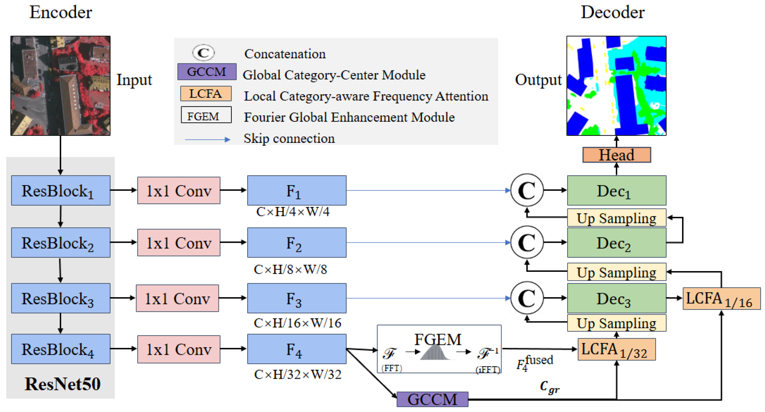
The proposed GC2F-Net adopts an encoder–decoder architecture, and its overall framework is illustrated in Figure 1. In the encoding stage, ResNet-50 is employed as the backbone network to progressively extract hierarchical features through four residual stages, and a convolutional layer is introduced after each stage for channel alignment, thereby generating multiscale features for subsequent decoding and feature fusion. In the decoding stage, the GCCM is used to construct a category prior and provide category-level semantic constraints for subsequent decoding, while the FGEM performs frequency-domain enhancement on deep features to improve global structural representation and texture-detail modeling. Under the guidance of the category prior, the LCFA optimizes feature representations through local category-aware interaction and feature recalibration. Through the collaborative effects of the above modules, the model can effectively integrate global semantics and local details during the progressive restoration of spatial resolution. From an intuitive perspective, GCCM, FGEM, and LCFA are introduced to address category inconsistency, insufficient global structural representation, and detail degradation. In addition, skip connections are introduced between the encoder and decoder to concatenate features at corresponding scales along the channel dimension, thereby alleviating the loss of details caused by downsampling and enhancing the representation capability for target boundaries and structures.

Specifically, GC2F-Net employs the encoder to progressively extract multiscale features, which can be formulated as follows:

$${\mathbf{F}}_l={\mathcal{E}}_l\left({\mathbf{F}}_{l-1}\right),l=1,2,3,4,{\mathbf{F}}_0=\mathbf{I}.$$

(1)

where $\mathbf{I}\in {\mathbb{R}}^{C\times H\times W}$ denotes the input remote sensing image, and C, H and W represent the number of channels, height, and width. The ${\mathbf{F}}_l\in {\mathbb{R}}^{C\times H\times W}$ denotes the output feature at layer l, ${\mathcal{E}}_l(·)$ represents the mapping function of the corresponding residual stage, and l is the stage index.

GC2F-Net constructs a category prior on the deepest features, and the overall mapping of GCCM is formulated as follows:

$${\mathbf{C}}_{\mathrm{gr}}=\mathcal{G}\left({\mathbf{F}}_4\right).$$

(2)

where $\mathcal{G}(·)$ denotes the mapping function of GCCM, and ${\mathbf{C}}_{\mathrm{gr}}\in {\mathbb{R}}^{K\times C}$ represents the global category-center matrix after frequency-guided channel recalibration, where K denotes the number of classes and C denotes the channel dimension of the category centers.

Meanwhile, the FGEM performs frequency-domain enhancement on the deep features and fuses them with the original features in a residual manner:

$${\mathbf{F}}_4^{\mathrm{fused}}={\mathbf{F}}_4+{\mathcal{F}}_{\mathrm{fg}}\left({\mathbf{F}}_4\right).$$

(3)

where ${\mathcal{F}}_{\mathrm{fg}}(·)$ denotes the nonlinear mapping of the FGEM, and ${\mathbf{F}}_4^{\mathrm{fused}}$ represents the deep feature after frequency-domain enhancement and residual fusion.

On this basis, LCFA takes ${\mathbf{F}}_4^{\mathrm{fused}}$ as input and introduces ${\mathbf{C}}_{\mathrm{gr}}$ as the category prior at the two scales of $1/32$ and $1/16$ to perform local category-aware interaction and modeling on local features, thereby enhancing the discriminative responses related to target categories and suppressing background interference during the progressive restoration of spatial resolution. Subsequently, the decoder restores spatial details through progressive upsampling, skip connections, and convolution operations, and finally outputs the pixel-level classification probability map.

3.2. Global Category-Center Module

During the decoding process of semantic segmentation, although deep features possess strong semantic representation capability, their information is still mainly organized at the pixel level and lacks explicit category-level priors that can be used to constrain the decoding process. As a result, category semantics are difficult to propagate stably and effectively to subsequent stages. To provide more stable semantic guidance, GCCM is introduced on the deepest feature ${\mathbf{F}}_4\in {\mathbb{R}}^{C\times H\times W}$ to explicitly construct image-adaptive category-center priors. 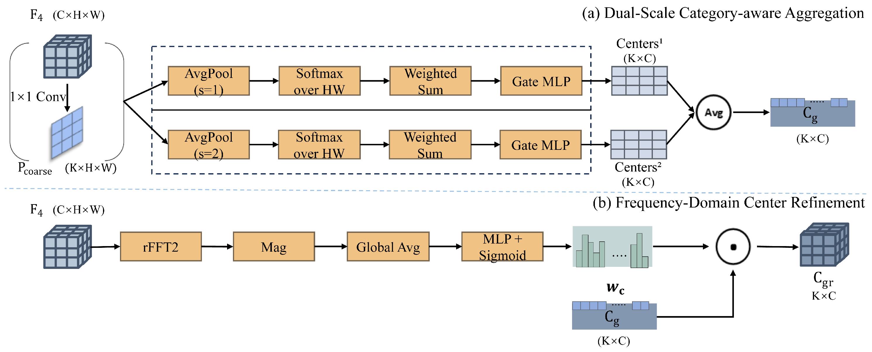As illustrated in Figure 2, the GCCM mainly consists of two parts, the Dual-Scale Category-aware Aggregation Module and the Frequency-Domain Center Refinement Module. The former performs category-aware aggregation on deep features in the spatial domain based on coarse-grained predictions, whereas the latter combines frequency-domain statistics to conduct global recalibration on the category centers. In this way, GCCM can be intuitively regarded as a category-level summarization mechanism, which converts dense pixel features into compact category centers and helps reduce background-induced category confusion during subsequent decoding.

Specifically, to improve the stability of the global category centers, the GCCM adopts a dual-scale branch to downsample the deep features and the coarse predictions, which can be formulated as follows:

$${\mathbf{F}}^{\left(s\right)}={\mathrm{AvgPool}}_s\left({\mathbf{F}}_4\right),{\mathbf{P}}^{\left(s\right)}={\mathrm{AvgPool}}_s\left({\mathbf{P}}_{\mathrm{coarse}}\right),s\in \{1,2\}.$$

(4)

where ${\mathbf{P}}_{\mathrm{coarse}}\in {\mathbb{R}}^{K\times H\times W}$ denotes the coarse-grained prediction map obtained from ${\mathbf{F}}_4$ through a $1\times 1$ convolution, which is used to generate category-aware aggregation weights; ${\mathrm{AvgPool}}_s(·)$ denotes the average pooling operation at scale s; ${\mathbf{F}}^{\left(s\right)}\in {\mathbb{R}}^{C\times H_s\times W_s}$ and ${\mathbf{P}}^{\left(s\right)}\in {\mathbb{R}}^{K\times H_s\times W_s}$ denote the feature map and the coarse-grained prediction map at scale s, respectively, where $s=1$ denotes the original-scale branch and $s=2$ denotes the downsampled branch; C denotes the number of channels; and K denotes the number of categories.

After obtaining the feature ${\mathbf{F}}^{\left(s\right)}$ and the coarse-grained prediction ${\mathbf{P}}^{\left(s\right)}$ at scale s, in order to construct category-aware aggregation weights along the spatial dimension, Softmax normalization is first applied to ${\mathbf{P}}^{\left(s\right)}$ over the spatial dimension, thereby obtaining the weight distribution of each category at different spatial locations:

$$a_{k,i}^{\left(s\right)}={\displaystyle \frac{\exp \left(p_{k,i}^{\left(s\right)}\right)}{{\sum }_{j=1}^{N_s}\exp \left(p_{k,j}^{\left(s\right)}\right)}},i=1,\dots ,N_s,k=1,\dots ,K,s\in \{1,2\}.$$

(5)

where $p_{k,i}^{\left(s\right)}$ denotes the prediction score of the i spatial location belonging to the k category at scale s, $a_{k,i}^{\left(s\right)}$ denotes the corresponding category-aware aggregation weight, and $N_s=H_s{W}_s$ is the number of spatial locations.

Subsequently, the above weights are used to perform weighted aggregation of the features, thereby obtaining the category center of the k category at scale s:

$${\mathbf{c}}_k^{\left(s\right)}={\displaystyle \sum _{i=1}^{N_s}}{a}_{k,i}^{\left(s\right)}{\mathbf{f}}_i^{\left(s\right)},k=1,\dots ,K.$$

(6)

where ${\mathbf{f}}_i^{\left(s\right)}\in {\mathbb{R}}^C$ denotes the feature vector at the i spatial location at scale s, and ${\mathbf{c}}_k^{\left(s\right)}\in {\mathbb{R}}^C$ denotes the category center of the k category at scale s. By stacking all category centers along the category dimension, the category-center matrix ${\mathbf{C}}^{\left(s\right)}\in {\mathbb{R}}^{K\times C}$ is obtained. Subsequently, a lightweight nonlinear transformation and gating operation are applied to ${\mathbf{C}}^{\left(s\right)}$ to suppress noisy categories and enhance the representation of effective categories. Finally, the dual-scale category centers are fused to obtain the initial global category centers:

$${\mathbf{C}}_{\mathrm{g}}={\displaystyle \frac{1}{\left|S\right|}}\sum _s{\mathbf{C}}^{\left(s\right)},s\in \{1,2\}.$$

(7)

where ${\mathbf{C}}_{\mathrm{g}}\in {\mathbb{R}}^{K\times C}$ denotes the initial global category centers obtained by dual-scale fusion, and $\left|S\right|$ denotes the number of scale branches.

Furthermore, the Frequency-Domain Center Refinement Module takes ${\mathbf{F}}_4$ as input and first performs a two-dimensional real-valued Fourier transform on it to obtain the frequency-domain representation ${\widehat{\mathbf{F}}}_4=\mathcal{F}\left({\mathbf{F}}_4\right)$. Subsequently, its amplitude spectrum $\mathbf{M}=|{\widehat{\mathbf{F}}}_4|$ is computed, and the channel-wise frequency-domain statistical information $\mathbf{z}=\mathrm{GAP}\left(\mathbf{M}\right)$ is extracted through global average pooling. On this basis, an MLP and a Sigmoid function are employed to generate the channel weight vector $\mathbf{w}=\mathrm{MLP}\left(\mathbf{z}\right)$, which is then applied to the initial global category centers ${\mathbf{C}}_{\mathrm{g}}\in {\mathbb{R}}^{K\times C}$ for channel recalibration, thereby yielding the frequency-refined global category centers ${\mathbf{C}}_{\mathrm{gr}}\in {\mathbb{R}}^{K\times C}$. This process enables the category centers to more fully encode the key frequency information contained in the deep features, thereby improving their representation stability and cross-scene generalization capability.

$${\left({\mathbf{C}}_{\mathrm{g}r}\right)}_{k,c}=w_c{\left({\mathbf{C}}_{\mathrm{g}}\right)}_{k,c}.$$

(8)

where k and c denote the category index and channel index, respectively, and $w_c$ denotes the weight of the c channel predicted from the frequency-domain statistics. Through the above frequency-guided channel recalibration, the model is able to enhance the responses of discriminative frequency-domain channels, thereby obtaining more robust global category-center priors. In this way, the GCCM provides explicit category-level constraints for subsequent feature updates during the decoding stage, enabling the category prior to effectively participate in the subsequent pixel-level interaction.

3.3. Fourier Global Enhancement Module

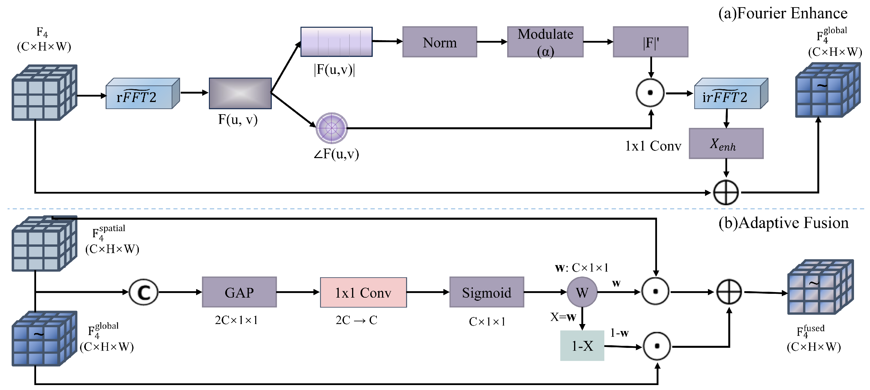
Since the category prior mainly provides semantic constraints at the level of category vectors, it is insufficient to directly enhance global structural representations at the feature-map level. Therefore, it is necessary to introduce a frequency-domain enhancement branch at the feature-map level to perform global enhancement on deep features. Intuitively, GCCM provides category-level guidance on what semantic regions should be emphasized, whereas FGEM further enhances how global structures and texture-related frequency responses are represented in the deep feature map. As shown in Figure 3, Different from the global category-center priors constructed by the GCCM, the FGEM operates directly on the deep feature map ${\mathbf{F}}_4\in {\mathbb{R}}^{C\times H\times W}$ of the encoder. While preserving the spatial resolution, it exploits frequency-domain information to enhance global structural representation and adaptively fuses it with the original spatial features, thereby strengthening structural and detail cues without replacing the original spatial representation, and finally outputs the deep feature representation ${\mathbf{F}}_4^{\mathrm{fused}}$ for subsequent decoding and for the LCFA.

Overall, the FGEM can be regarded as a nonlinear transformation applied to the deep encoder feature ${\mathbf{F}}_4\in {\mathbb{R}}^{C\times H\times W}$. Specifically, a two-dimensional real-valued Fourier transform (rFFT2) with orthogonal normalization is first performed on the ${\mathbf{F}}_4$ channel by channel along the spatial dimensions, yielding the complex spectrum:

$$\widehat{\mathbf{F}}(u,v)=\mathcal{F}\left({\mathbf{F}}_4(x,y)\right).$$

(9)

where $\mathcal{F}(·)$ denotes the two-dimensional real-valued Fourier transform, and $\widehat{\mathbf{F}}(u,v)$ denotes the corresponding complex-valued frequency-domain representation. The complex spectrum is then decomposed into the amplitude spectrum and the phase spectrum:

$$\mathbf{A}=|\widehat{\mathbf{F}}(u,v)|,\mathit{\varphi }=\arg \left(\widehat{\mathbf{F}}(u,v)\right).$$

(10)

where $\mathbf{A}$ and $\mathit{\varphi }$ denote the amplitude spectrum and phase spectrum, respectively.

To preserve spatial structural information, the FGEM keeps the phase spectrum $\mathit{\varphi }$ unchanged and only modulates the amplitude spectrum $\mathbf{A}$. For each sample and channel, the amplitude spectrum is normalized over the frequency plane as:

$${\mu }_{b,c}={\mathrm{Mean}}_{(u,v)\in \Omega }\left({\mathbf{A}}_{b,c,u,v}\right),{\sigma }_{b,c}={\mathrm{Std}}_{(u,v)\in \Omega }\left({\mathbf{A}}_{b,c,u,v}\right)+ϵ,{\mathbf{A}}_{b,c,u,v}^{\mathrm{norm}}={\displaystyle \frac{{\mathbf{A}}_{b,c,u,v}-{\mu }_{b,c}}{{\sigma }_{b,c}}}.$$

(11)

where b and c denote the sample index and channel index, respectively, $\Omega$ denotes the set of frequency coordinates, and $ϵ={10}^{-5}$ is used for numerical stability.

The normalized amplitude spectrum is then modulated by a bounded gated function:

$${\tilde{\mathbf{A}}}_{b,c,u,v}={\mathbf{A}}_{b,c,u,v}\left[1+\alpha \tanh \left({\mathbf{A}}_{b,c,u,v}^{\mathrm{norm}}\right)\right].$$

(12)

where $\alpha$ is a learnable scalar parameter initialized to 0, which controls the modulation strength of the amplitude spectrum.

The modulated amplitude spectrum is recombined with the original phase spectrum and transformed back to the spatial domain:

$$\tilde{\mathbf{F}}(u,v)=\tilde{\mathbf{A}}(u,v)\exp \left(j\mathit{\varphi }(u,v)\right),{\mathbf{X}}_{\mathrm{enh}}={\mathcal{F}}^{-1}\left(\tilde{\mathbf{F}}(u,v)\right).$$

(13)

Finally, the enhanced feature is mapped by a learnable $1\times 1$ convolution and fused with the input feature through a residual connection:

$${\mathbf{F}}_4^{\mathrm{global}}={\mathbf{F}}_4+{\mathrm{Conv}}_{1\times 1}\left({\mathbf{X}}_{\mathrm{enh}}\right),{\mathbf{F}}_4^{\mathrm{global}}\in {\mathbb{R}}^{C\times H\times W}.$$

(14)

where ${\mathrm{Conv}}_{1\times 1}(·)$ denotes a learnable channel-mapping convolution.

Although the frequency-domain global branch enhances global structural representation, the original spatial features still preserve local textures and edge details. Therefore, a lightweight channel-adaptive fusion strategy is adopted. The spatial-branch feature ${\mathbf{F}}_4^{\mathrm{spatial}}$ and the global-branch feature ${\mathbf{F}}_4^{\mathrm{global}}$ are concatenated, followed by global average pooling, a learnable $1\times 1$ convolution, and a Sigmoid function to generate the channel weight $\mathbf{w}$. The fused feature is obtained as

$${\mathbf{F}}_4^{\mathrm{fused}}=\mathbf{w}\odot {\mathbf{F}}_4^{\mathrm{spatial}}+\left(\mathbf{1}-\mathbf{w}\right)\odot {\mathbf{F}}_4^{\mathrm{global}}.$$

(15)

where ${\mathbf{F}}_4^{\mathrm{spatial}}={\mathbf{F}}_4$, ⊙ denotes element-wise multiplication, and $\mathbf{w}\in {(0,1)}^{C\times 1\times 1}$ denotes the channel-wise fusion weight. Through this design, the FGEM provides enhanced deep representations for subsequent multiscale decoding and the LCFA.

3.4. Local Category-Aware Frequency Attention Module

Category prior can provide explicit category-level constraints for the decoding process. However, if it is merely treated as additional input information, it is often difficult for the category prior to establish an explicit correspondence with pixel-level discrimination, especially in boundary regions and small-object regions, where category confusion and background-induced false responses are more likely to occur. Therefore, the key purpose of LCFA is to make the category prior directly participate in local feature refinement rather than only serving as auxiliary global information. 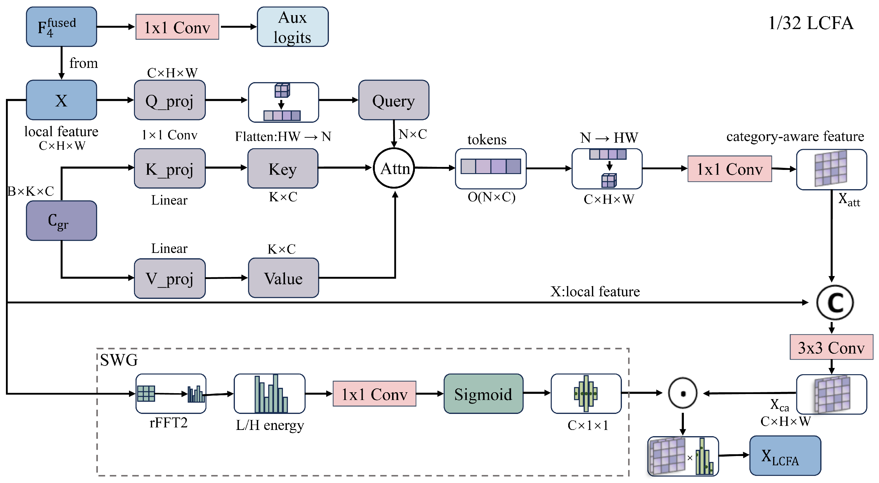To address this issue, LCFA is introduced at the $1/32$ and $1/16$ scales during the decoding stage. This module injects the category prior into the local feature updating process through pixel-category center interaction, and recalibrates feature responses by incorporating frequency statistics, thereby improving the discrimination capability for fine-grained structures. In this way, each spatial position can adaptively select relevant category-center information under global semantic guidance, which helps refine ambiguous boundaries and small-object regions. The architecture of the LCFA at the $1/32$ scale is illustrated in Figure 4.

First, the input features are projected into pixel tokens, while the global category-centers are projected into category tokens. Specifically, a $1\times 1$ convolution is applied to the local feature $\mathbf{X}$, followed by flattening along the spatial dimension to generate the Query. Meanwhile, a linear projection is performed on the global category-centers ${\mathbf{C}}_{\mathrm{gr}}$ to generate the Key and Value:

$$\begin{array}{cc}\hfill \mathbf{Query}& =\mathrm{Flatten}\left({\mathrm{Conv}}_{1\times 1}\left(\mathbf{X}\right)\right)\in {\mathbb{R}}^{N\times C},N=H\times W,\hfill \\ \hfill \mathbf{Key}& ={\varphi }_{\mathrm{K}}\left({\mathbf{C}}_{\mathrm{gr}}\right),\mathbf{Value}={\varphi }_{\mathrm{V}}\left({\mathbf{C}}_{\mathrm{gr}}\right),\mathbf{Key},\mathbf{Value}\in {\mathbb{R}}^{K\times C}.\hfill \end{array}$$

(16)

where ${\mathrm{Conv}}_{1\times 1}(·)$ denotes the $1\times 1$ convolution used for channel projection, $\mathrm{Flatten}(·)$ denotes the flattening operation over the spatial dimensions, and ${\varphi }_{\mathrm{K}}(·)$ and ${\varphi }_{\mathrm{V}}(·)$ denote the linear projection functions.

Subsequently, category-level attention is performed by taking the pixel tokens as the Query and the category tokens as the Key and Value, followed by Softmax normalization along the category dimension, so that each spatial position can adaptively select the relevant category centers and aggregate them to obtain a category-aware representation:

$$\mathbf{A}=\mathrm{Softmax}\left({\displaystyle \frac{\mathbf{Q}{\mathbf{K}}^{\mathrm{T}}}{\sqrt{C}}}\right)\in {\mathbb{R}}^{N\times K},\mathbf{O}=\mathbf{A}\mathbf{V}\in {\mathbb{R}}^{N\times C}.$$

(17)

where $\sqrt{C}$ is the scaling factor, $\mathbf{A}\in {\mathbb{R}}^{N\times K}$ denotes the association weights between pixel tokens and category centers, and $\mathbf{O}\in {\mathbb{R}}^{N\times C}$ denotes the category-aware feature representation obtained by weighted aggregation of the category value tokens.

Next, $\mathbf{O}$ is restored to the spatial layout and passed through a $1\times 1$ convolution to obtain the category-aware feature ${\mathbf{X}}_{\mathrm{att}}\in {\mathbb{R}}^{C\times H\times W}$. To preserve local texture details while injecting the category prior, the LCFA concatenates ${\mathbf{X}}_{\mathrm{att}}$ and the original feature $\mathbf{X}$ along the channel dimension, and then applies a $3\times 3$ convolution to obtain the category-enhanced feature:

$${\mathbf{X}}_{\mathrm{ca}}={\mathrm{Conv}}_{3\times 3}\left(\mathrm{Cat}(\mathbf{X},{\mathbf{X}}_{\mathrm{att}})\right)\in {\mathbb{R}}^{C\times H\times W}.$$

(18)

where $\mathrm{Cat}(·)$ denotes concatenation along the channel dimension, and ${\mathrm{Conv}}_{3\times 3}(·)$ is used for detail compensation. It can be observed that, different from the GCCM, which mainly performs recalibration at the category level, the LCFA explicitly establishes the correspondence between local features and category centers at the pixel level, enabling each spatial position to adaptively select more relevant category-center information under the guidance of category prior, thereby enhancing the responses of target regions and suppressing background interference. In addition, an auxiliary prediction map is generated within the module for auxiliary supervision during the training stage.

Relying on spatial attention is insufficient to characterize the differences in the roles of different channels in frequency structures. To this end, a Spectral-weight Gating Module (SWG) is introduced into the LCFA to perform joint recalibration of channels and frequencies on ${\mathbf{X}}_{\mathrm{ca}}$. Specifically, a two-dimensional real-valued Fourier transform is first applied to the input feature to obtain the amplitude spectrum. Subsequently, the average responses of the low-frequency band and the high-frequency band are computed separately, and their ratio is used to construct a channel-wise frequency descriptor. Finally, a channel gating weight $\mathbf{g}$ is generated through a lightweight mapping and a Sigmoid activation, which is used to modulate the category-enhanced feature in a channel-wise manner, thereby yielding the output of the LCFA:

$${\mathbf{X}}_{\mathrm{LCFA}}=\mathbf{g}\odot {\mathbf{X}}_{\mathrm{ca}}.$$

(19)

where $\mathbf{g}\in {\mathbb{R}}^{C\times 1\times 1}$ denotes the channel gating weight, and ⊙ denotes element-wise multiplication. When the high-frequency energy of a certain channel within a local window is significantly higher than its low-frequency energy, the SWG assigns a larger weight to that channel so as to emphasize structure-sensitive components such as edges and textures; conversely, channels with weaker frequency-domain contributions or those dominated by noise are suppressed. Different from the image-level spectral modulation in the FGEM, the SWG in the LCFA operates on decoding-stage features in a window-based manner, making it more suitable for characterizing local details and target boundaries.

In the network, one LCFA layer is applied at the $1/32$ scale by taking ${\mathbf{F}}_4^{\mathrm{fused}}$ as input to obtain deep category-aware enhanced features. Subsequently, another LCFA layer is applied at the $1/16$ scale to the upsampled intermediate-level features. The two scales share the same set of global category centers ${\mathbf{C}}_{\mathrm{gr}}$, but model local–global interaction separately under different spatial resolutions, thereby enabling the category prior to be progressively propagated to finer-grained spatial locations. The outputs of the multiscale LCFA are fused with shallow detailed features through skip connections and upsampling operations, and are then passed to the final prediction head to produce the pixel-level segmentation results.

4. Experiments

4.1. Datasets

To evaluate the proposed method, experiments were conducted on three representative semantic segmentation datasets, namely ISPRS Vaihingen (ISPRS 2D Semantic Labeling Benchmark: https://www.isprs.org/resources/datasets/benchmarks/UrbanSemLab/semantic-labeling.aspx, (accessed on 9 May 2026), ISPRS Potsdam (ISPRS 2D Semantic Labeling Benchmark: https://www.isprs.org/resources/datasets/benchmarks/UrbanSemLab/semantic-labeling.aspx, (accessed on 9 May 2026), and UAVid (UAVid dataset: https://uavid.nl/, (accessed on 9 May 2026). These datasets differ substantially in terms of imaging platform, viewing perspective, spatial resolution, and scene complexity, thereby providing a comprehensive benchmark for evaluating the generalization capability and robustness of the proposed model under diverse scene conditions.

The ISPRS Vaihingen dataset consists of high-resolution aerial orthophotos acquired over Vaihingen, Germany, together with pixel-level annotations. It has a spatial resolution of 9 cm and mainly covers typical urban scenes. Following the commonly used setting, a six-class semantic segmentation task was conducted, including impervious surfaces, buildings, low vegetation, trees, cars, and clutter. For dataset partitioning, images with IDs 1, 3, 5, 7, 11, 13, 15, 17, 21, 23, 26, 28, 32, 34, and 37 were used for training, image 30 was used for validation, and the remaining 17 images were used for testing. The original large-format images were cropped into patches of $512\times 512$ pixels as model inputs.

The ISPRS Potsdam dataset, also released by ISPRS, is a widely used benchmark for high-resolution remote sensing image semantic segmentation. It consists of 38 aerial images with a spatial resolution of 5 cm, and each original image is approximately $6000\times 6000$ pixels in size. The dataset follows the same six-class annotation scheme as the Vaihingen dataset. For dataset partitioning, images with IDs 2_11, 2_12, 3_10, 3_11, 3_12, 4_10, 4_11, 4_12, 5_10, 5_11, 5_12, 6_7, 6_8, 6_9, 6_10, 6_11, 6_12, 7_7, 7_8, 7_9, 7_10, 7_11, and 7_12 were used for training, image 2_10 was used for validation, and the remaining 14 images were used for testing. The original large-format images were cropped into patches of $512\times 512$ pixels as model inputs.

The UAVid dataset is a widely used high-resolution UAV image dataset for urban scene semantic segmentation. It is captured from an oblique viewing perspective and contains complex urban elements, including roads, buildings, vehicles, pedestrians, and vegetation. The dataset consists of 42 video sequences, from which annotated image frames are extracted, and is annotated into eight semantic classes. Following the official sequence-based split, 20 sequences were used for training, 7 sequences were used for validation, and the remaining 15 sequences were used for testing. The original 4K images were cropped into patches of $512\times 512$ pixels as model inputs.

4.2. Implementation Details

All experiments were conducted on a workstation equipped with an NVIDIA RTX 3090 GPU. The proposed model was implemented based on the PyTorch deep learning framework (v2.1.0) with Python (v3.10) and CUDA (v12.1). deep learning framework. ResNet-50 was adopted as the encoder backbone, upon which GC2F-Net was constructed. Unless otherwise specified, the input images were cropped into patches of $512\times 512$ pixels, and the batch size was set to 6.

For training, the AdamW optimizer was adopted, with the initial learning rate and weight decay set to $1\times {10}^{-4}$ and $1\times {10}^{-2}$, respectively. The number of training epochs was set to 150 for Vaihingen, 80 for Potsdam, and 80 for UAVid. The learning rate was updated using a polynomial decay strategy with the power set to 0.9. In addition, 1000 warm-up iterations were introduced at the early stage of training to improve training stability. For data augmentation, in addition to basic normalization, random horizontal and vertical flipping, random rotation, and geometric transformations were applied during training. Moreover, additional random cropping and flipping were performed on image patches containing relatively many vehicle targets to alleviate the training bias caused by the insufficient samples of small-object categories.

4.3. Evaluation Metrics

To comprehensively evaluate the performance of the proposed model in semantic segmentation tasks, mean Intersection over Union (mIoU), Overall Accuracy (OA), and mean F1-score (mF1) are adopted as the overall evaluation metrics, while the IoU of each category is also reported. Specifically, mIoU is used to measure the regional overlap between the predictions and the ground-truth annotations, OA reflects the overall classification accuracy over all pixels, and mF1 more comprehensively characterizes the overall segmentation performance across different categories. The above metrics are calculated as follows:

$$\begin{array}{cc}\hfill \mathrm{mIoU}& ={\displaystyle \frac{1}{N}}{\displaystyle \sum _{k=1}^N}{\displaystyle \frac{T{P}_k}{T{P}_k+F{P}_k+F{N}_k}},\hfill \\ \hfill \mathrm{OA}& ={\displaystyle \frac{{\sum }_{k=1}^{N}T{P}_k}{{\sum }_{k=1}^N(T{P}_k+F{P}_k)}},\hfill \\ \hfill \mathrm{mF}1& ={\displaystyle \frac{1}{N}}{\displaystyle \sum _{k=1}^N}{\displaystyle \frac{2{\mathrm{Precision}}_k{\mathrm{Recall}}_k}{{\mathrm{Precision}}_k+{\mathrm{Recall}}_k}}.\hfill \end{array}$$

(20)

where N denotes the number of valid categories, and $T{P}_k$, $F{P}_k$, and $F{N}_k$ denote the numbers of true positives, false positives, and false negatives for category k, respectively. ${\mathrm{Precision}}_k$ and ${\mathrm{Recall}}_k$ denote the precision and recall of category k, respectively, which are defined as ${\mathrm{Precision}}_k={\displaystyle \frac{T{P}_k}{T{P}_k+F{P}_k}}$ and ${\mathrm{Recall}}_k={\displaystyle \frac{T{P}_k}{T{P}_k+F{N}_k}}$.

4.4. Loss Function

To jointly account for pixel-wise classification accuracy and region-level overlap quality, the weighted sum of the cross-entropy (CE) loss and the multiclass Dice loss is adopted as the training objective. The CE loss facilitates stable optimization of pixel-wise category prediction, whereas the Dice loss constrains the consistency between the predicted regions and the ground-truth annotations and generally exhibits stronger robustness to class imbalance. The overall loss is formulated as follows:

$$\mathcal{L}={\lambda }_{\mathrm{ce}}{\mathcal{L}}_{\mathrm{ce}}+{\lambda }_{\mathrm{dice}}{\mathcal{L}}_{\mathrm{dice}}.$$

(21)

where ${\lambda }_{\mathrm{ce}}=1.0$, and ${\lambda }_{\mathrm{dice}}$ is initially set to $0.3$ and gradually adjusted to $0.4$ during training to impose a stronger constraint on region-level overlap. The cross-entropy loss is defined as:

$${\mathcal{L}}_{\mathrm{ce}}=-{\displaystyle \frac{1}{|\Omega |}}\sum _{i\in \Omega }\log p_{i,y_i}.$$

(22)

where $\Omega$ denotes the set of valid pixels, and $p_{i,y_i}$ denotes the predicted probability of pixel i for its ground-truth category. Unlabeled invalid pixels are ignored in the loss computation and excluded from backpropagation. The Dice loss is used to measure the regional overlap between the predictions and the annotations. In implementation, Softmax is first applied to the logits to obtain probabilities, and a mask is then imposed on invalid pixel positions to exclude them from the statistics. Subsequently, the Dice value is computed for each category and averaged. The multiclass Dice loss is defined as:

$${\mathcal{L}}_{\mathrm{dice}}=1-{\displaystyle \frac{1}{C}}{\displaystyle \sum _{c=1}^C}{\displaystyle \frac{2{\sum }_{i\in \Omega }{p}_{i,c}{g}_{i,c}+ϵ}{{\sum }_{i\in \Omega }{p}_{i,c}^2+{\sum }_{i\in \Omega }{g}_{i,c}^2+ϵ}}.$$

(23)

where C denotes the number of categories, $g_{i,c}$ denotes the ground-truth label in one-hot form, and $ϵ$ denotes the smoothing term. In implementation, the Dice loss is computed using squared terms.

5. Results

5.1. Comparative Experiments

Unless otherwise specified, all comparison methods are evaluated under the same training and inference settings described in Section 3.2 and with the same evaluation metrics. To verify the effectiveness of GC2F-Net, comparative experiments are conducted on the three datasets against several representative methods, including DANet [19], DeepLabV3 [35], FPN [17], PSPNet [15], OCRNet [20], SegFormer-R50 [26], and UNetFormer [27]. Specifically, SegFormer-R50 refers to a ResNet-50 encoder combined with a SegFormer-inspired decoding head. This setting was used to keep the backbone consistent with other ResNet-50-based comparison methods, enabling a controlled comparison under the same encoder configuration. Therefore, SegFormer-R50 should be regarded as a ResNet-50-based controlled variant, rather than the original Transformer-based SegFormer architecture.

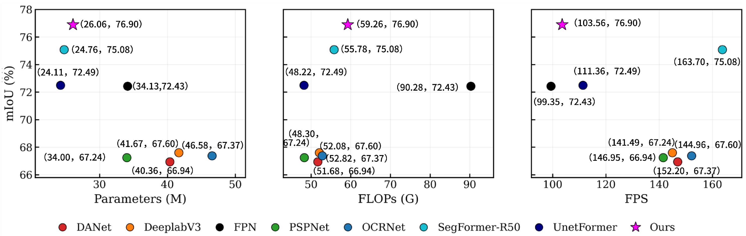
In addition to segmentation accuracy, the model complexity and inference efficiency of different methods are compared to more comprehensively evaluate the trade-off between accuracy and efficiency. It should be noted that the number of parameters, FLOPs, and FPS are mainly determined by the model architecture and the unified testing settings, and therefore remain consistent across different datasets, whereas mIoU varies with the dataset. To avoid repeatedly presenting the same efficiency axis ranges, the ISPRS Vaihingen dataset is selected for visualization to illustrate the distribution of different methods in terms of accuracy and efficiency.

As shown in Figure 5 and

Table 1. Performance–efficiency comparison on the ISPRS Vaihingen dataset.

Method	Params (M)	FLOPs (G)	FPS (img/s)	mIoU (%)
DANet	40.36	51.68	146.95	66.94
DeeplabV3	41.67	52.08	144.96	67.60
FPN	34.13	90.28	99.35	72.43
PSPNet	34.00	48.30	141.49	67.24
OCRNet	46.58	52.82	152.20	67.37
SegFormer-R50	24.76	55.78	163.70	75.08
UnetFormer	24.11	48.22	111.36	72.49
Ours	26.06	59.26	103.56	76.90

, GC2F-Net achieves the best segmentation performance, with an mIoU of 76.90% and 26.06 M parameters. Compared with other representative methods, the proposed model obtains a favorable balance between segmentation accuracy and model efficiency. In terms of computational cost, GC2F-Net requires 59.26 G FLOPs and reaches 103.56 img/s, showing acceptable inference efficiency under the same evaluation setting. Overall, GC2F-Net achieves a competitive performance–efficiency trade-off among segmentation accuracy, model size, and inference speed, which further demonstrates its effectiveness for high-resolution remote sensing semantic segmentation.

5.1.1. Vaihingen Dataset

On the ISPRS Vaihingen dataset, as shown in

Table 2. Quantitative comparison on the ISPRS Vaihingen dataset (%). Bold values indicate the best result in each column.

Method	Backbone	Per-Class IoU (%)						mIoU (%)	mF1 (%)	OA (%)
		ImSurf	Bui.	LowVeg	Tree	Car	Clutter
DANet	ResNet-50	83.35	89.51	71.21	80.47	49.18	27.89	66.94	77.89	89.42
DeeplabV3	ResNet-50	83.78	89.69	70.75	80.38	45.73	35.26	67.60	78.77	89.50
FPN	ResNet-50	86.44	90.86	73.81	82.40	77.70	23.36	72.43	81.42	90.92
PSPNet	ResNet-50	83.76	89.77	71.41	80.54	47.37	30.63	67.24	78.25	89.60
OCRNet	ResNet-50	84.24	90.29	72.07	80.46	47.20	29.96	67.37	78.25	89.81
SegFormer-R50	ResNet-50	87.18	91.35	73.58	82.36	79.81	36.20	75.08	84.28	91.16
UnetFormer	ResNet-50	86.55	90.01	72.26	82.02	75.88	28.23	72.49	81.98	90.60
Ours	ResNet-50	87.91	92.06	74.21	82.79	81.11	43.29	76.90	85.86	91.56

, GC2F-Net achieves the best overall performance among the compared methods. The mIoU, mF1, and OA reach 76.90%, 85.86%, and 91.56%, respectively. Compared with SegFormer-R50, which is the strongest competing method, GC2F-Net improves mIoU, mF1, and OA by 2.34%, 1.27%, and 0.86%, respectively. These results indicate that the proposed method exhibits clear advantages in both overall segmentation accuracy and category consistency.

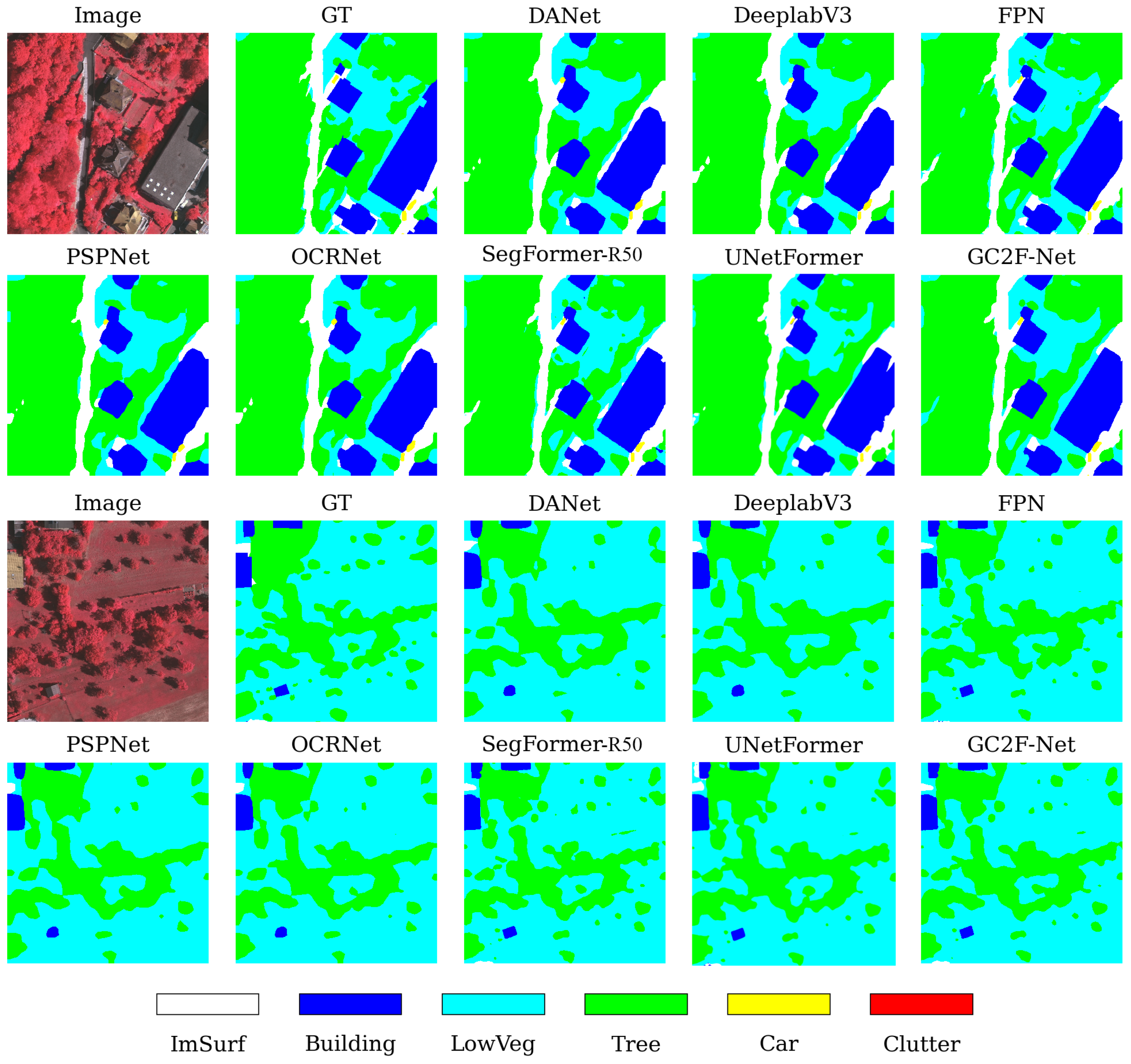
From the category-level results, GC2F-Net performs particularly well on the Building and Car classes, indicating that the proposed model possesses stronger structural representation and fine-grained discrimination capabilities for regular-structure targets and small-scale objects. Meanwhile, it also outperforms the other compared methods on the Clutter category, demonstrating higher robustness in complex backgrounds and unstructured regions. As shown in Figure 6, GC2F-Net produces smoother and more coherent segmentation results in boundary regions and identifies small objects more accurately. In particular, in building edges and road regions, its predicted boundaries are more consistent with the ground truth (GT). In summary, GC2F-Net effectively preserves fine-grained details while improving category consistency, thereby achieving more reliable segmentation results.

5.1.2. Potsdam Dataset

On the Potsdam dataset, as shown in

Table 3. Quantitative comparison on the ISPRS Potsdam dataset (%). Bold values indicate the best result in each column.

Method	Backbone	Per-Class IoU (%)						mIoU (%)	mF1 (%)	OA (%)
		ImSurf	Bui.	LowVeg	Tree	Car	Clutter
DANet	ResNet-50	84.89	92.74	76.85	79.19	73.99	44.93	75.43	85.07	90.15
DeeplabV3	ResNet-50	82.49	90.56	75.91	78.70	69.90	38.59	72.69	82.97	89.03
FPN	ResNet-50	87.38	93.57	77.92	81.01	93.17	40.18	78.87	86.81	91.11
PSPNet	ResNet-50	85.28	92.60	76.54	79.53	77.33	41.96	75.54	84.98	90.16
OCRNet	ResNet-50	85.20	93.01	77.50	80.06	75.73	42.68	75.70	85.11	90.42
SegFormer-R50	ResNet-50	85.85	92.61	76.12	79.63	92.38	33.78	76.73	85.03	90.17
UnetFormer	ResNet-50	85.04	91.98	76.81	78.37	89.63	41.10	77.66	85.88	89.94
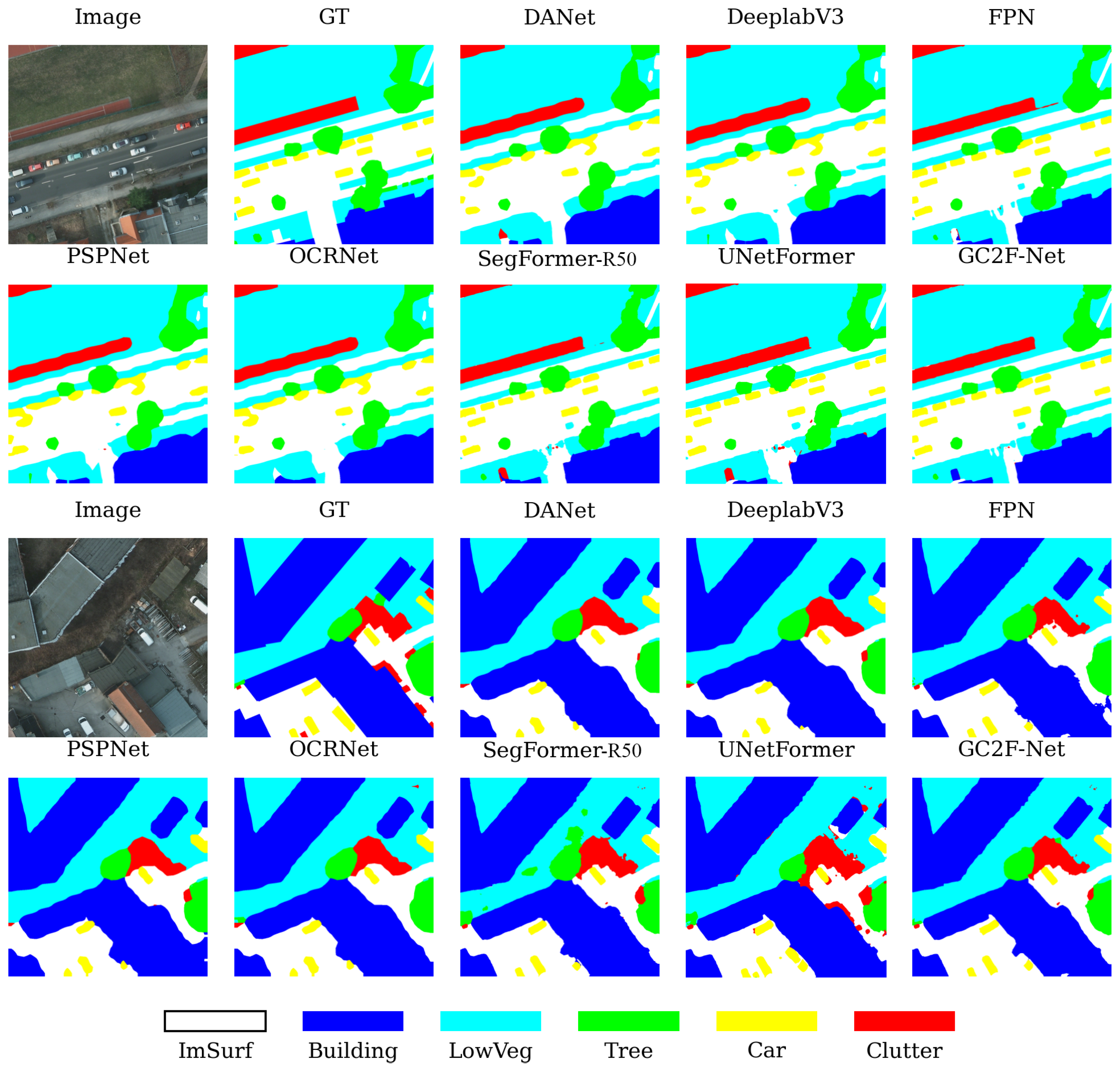
Ours	ResNet-50	87.67	93.93	78.39	79.59	92.82	44.26	79.44	87.41	91.23

, GC2F-Net achieves an mIoU, mF1, and OA of 79.44%, 87.41%, and 91.23%, respectively. Compared with FPN, which is the strongest competing method, the proposed method improves these three metrics by 0.57%, 0.60%, and 0.12%, respectively, indicating that it likewise exhibits favorable segmentation performance in this scene.

From the category-level results, GC2F-Net maintains strong competitiveness across multiple major categories and achieves better performance on key categories such as Bui and LowVeg, indicating that the proposed method can stably improve the segmentation accuracy of the main ground-object categories. Meanwhile, it also performs robustly on the complex background category Clutter, demonstrating its capability to suppress background interference and contributing to the improvement of overall mIoU and mF1. As shown in Figure 7, GC2F-Net produces more coherent prediction results over large-area regions with less fragmentation and presents clearer contours at boundary locations such as buildings and roads. In regions with adjacent vegetation and strong background interference, the category confusion phenomenon is effectively alleviated, indicating that the proposed method has advantages in both global context modeling and local detail recovery.

5.1.3. UAVid Dataset

As shown in

Table 4. Quantitative comparison on the UAVid dataset (%). Bold values indicate the best result in each column.

Method	Per-Class IoU (%)								mIoU (%)	mF1 (%)	OA (%)
	Bui.	Road	Tree	Veg.	Mo.Car	St.Car	Human	Clutter
DANet	90.83	76.19	76.89	67.47	56.22	52.73	12.36	64.71	62.18	73.85	87.17
DeeplabV3	91.45	77.17	77.26	67.63	55.68	56.19	14.59	65.35	63.17	74.81	87.49
FPN	91.17	78.26	77.33	68.33	62.06	56.65	27.23	65.76	65.85	77.83	87.69
PSPNet	90.94	77.00	76.80	67.19	56.01	57.34	14.41	65.24	63.12	74.80	87.30
OCRNet	90.99	76.90	76.71	68.60	53.01	52.32	11.57	64.52	61.80	73.44	87.27
SegFormer-R50	90.96	77.52	77.07	67.44	61.60	60.22	28.83	64.70	66.04	78.11	87.36
UNetFormer	90.93	77.60	77.56	68.70	68.40	59.45	19.82	63.90	65.80	77.29	87.53
Ours	91.04	77.65	77.28	68.67	68.22	63.10	25.57	64.81	67.04	78.65	87.63

, since the pixel-level ground-truth annotations (GT) of the UAVid test set are not publicly available, this paper follows the common evaluation protocol and conducts evaluation on the validation set. Overall, GC2F-Net achieves the best performance in terms of mIoU and mF1, reaching 67.04% and 78.65%, respectively, while the OA reaches 87.63%, indicating that the proposed method possesses strong overall segmentation capability and category consistency in complex urban scenes.

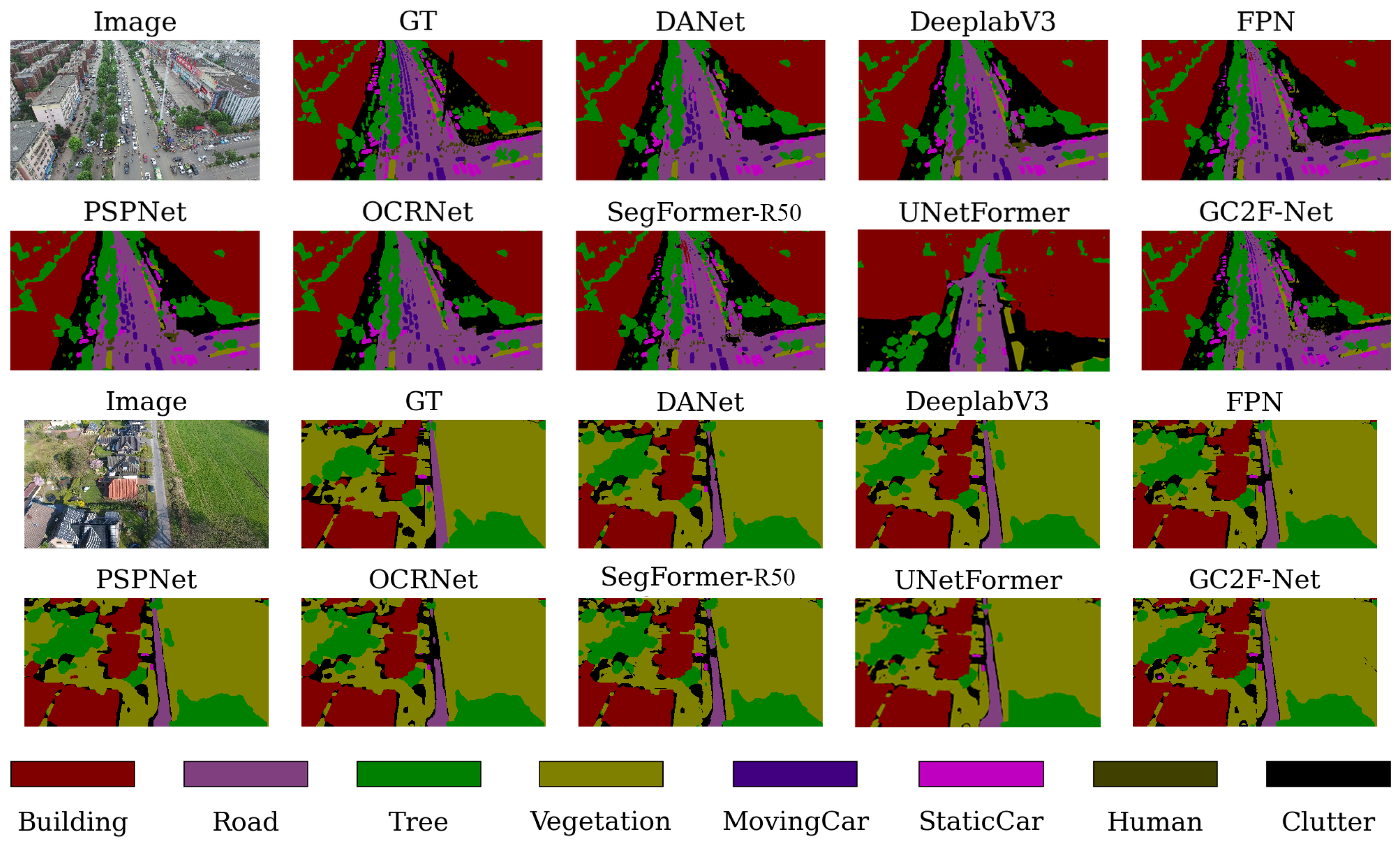
Figure 8 presents the qualitative comparison results on the UAVid dataset, from which it can be observed that GC2F-Net exhibits better connectivity and more accurate boundary localization for structured objects. It also effectively reduces structural discontinuities and boundary overflow in elongated regions and boundary transition areas. In addition, in small-object regions, its predictions are more consistent with the GT in spatial distribution, with reduced omission and misclassification errors. These results indicate that GC2F-Net possesses strong local detail recovery capability and stable category consistency in complex urban scenes. Meanwhile, due to factors such as the small scale of the Human category, complex shape variations, susceptibility to occlusion, and imbalanced category distribution, the IoU values of all methods for this category remain relatively low overall, whereas the proposed method still achieves results superior to those of most compared methods.

In summary, GC2F-Net not only achieves collaborative improvement in segmentation accuracy and robustness under complex scene conditions, but also alleviates the difficulty of jointly accounting for global context modeling and local detail representation in semantic segmentation of high-resolution remote sensing images. The experimental results demonstrate that the proposed method achieves stable and competitive performance on all three datasets, exhibiting favorable cross-dataset generalization capability.

5.2. Ablation Experiments

To verify the effectiveness of the key modules in GC2F-Net, namely GCCM, FGEM, and LCFA, and to analyze the contribution of each module to the overall performance improvement, ablation experiments are conducted. Considering that the variation trends of the experimental results are generally consistent across different datasets, the ISPRS Vaihingen dataset is selected in the main text for analysis. The baseline model (Baseline) is defined as follows: under the same backbone network and overall encoder–decoder framework, the GCCM, FGEM, and LCFA modules are removed, and only conventional multiscale feature extraction and decoding fusion are retained, thereby constructing a minimal comparison model without the proposed modules. Except for the module configuration, the remaining training and inference settings, data partitioning, and evaluation metrics are kept consistent with those used in the comparative experiments to ensure fairness and reproducibility.

As shown in

Table 5. Ablation experiments on the Vaihingen datasets.

Method	mIoU (%)	mF1 (%)	OA (%)	Parameters (M)	FLOPs (G)
Baseline	74.16	83.46	91.10	24.973	58.174
Baseline+GCCM	74.86	83.98	91.19	25.005	58.174
Baseline+FGEM	75.08	84.41	91.12	25.006	58.182
Baseline+LCFA	75.11	84.34	91.20	25.991	59.396
Full	76.90	85.86	91.56	26.056	59.405

, the complete model achieves 76.90%, 85.86%, and 91.56% in terms of mIoU, mF1, and OA, respectively, representing improvements of 2.74%, 2.40%, and 0.46% over the Baseline. These results indicate that the proposed modules significantly improve the overall segmentation accuracy and enhance category consistency. In terms of computational cost, compared with the baseline model, the complete model introduces only slight increases in the number of parameters and FLOPs, indicating that these performance gains are obtained with only a small additional computational overhead, thereby demonstrating a favorable trade-off between efficiency and accuracy.

5.2.1. Influence of Global Category-Center Module

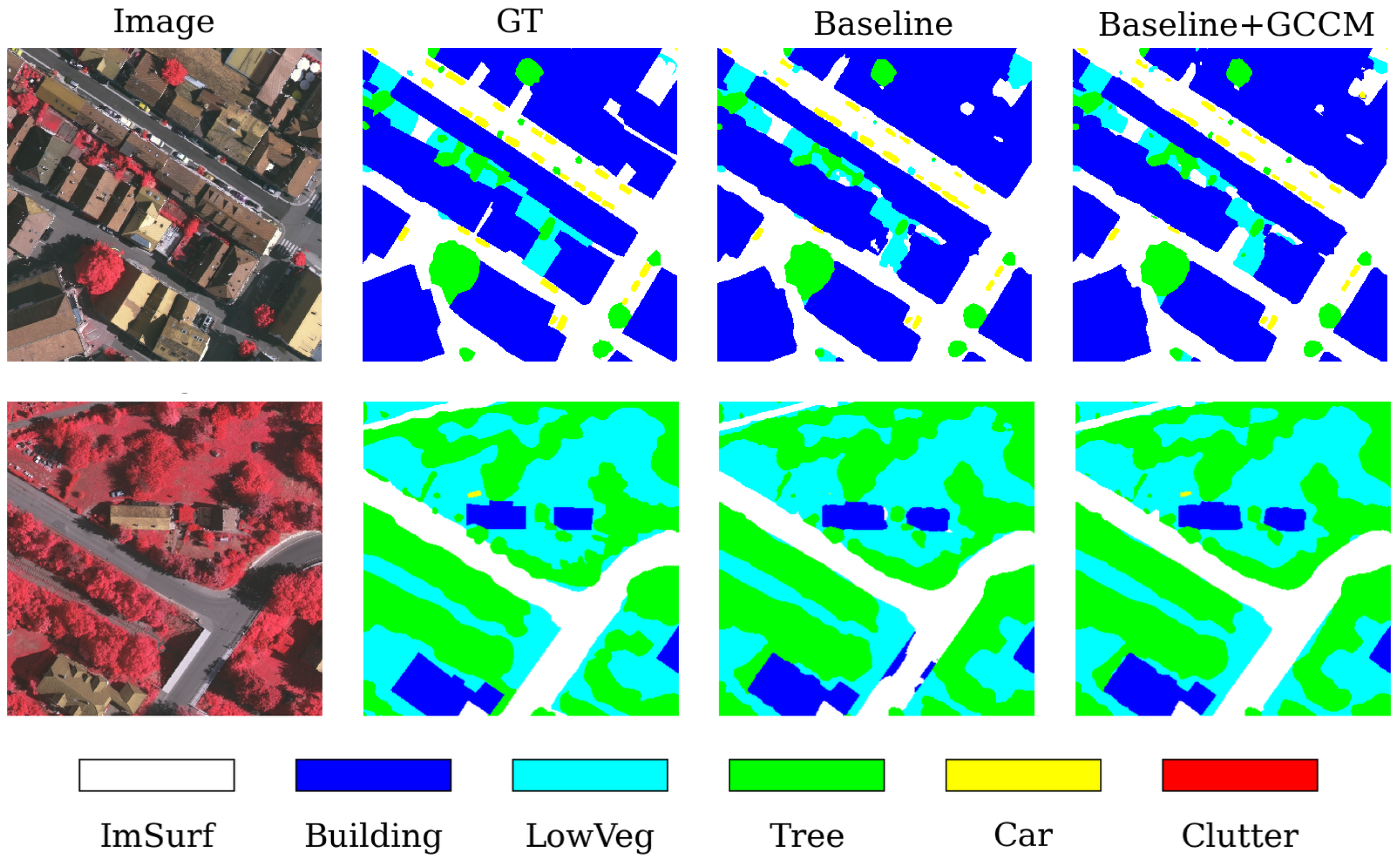
After introducing GCCM into the Baseline, mIoU increases from 74.16% to 74.86%, while mF1 and OA improve from 83.46% and 91.10% to 83.98% and 91.19%, respectively. These results indicate that global category-center modeling provides stable category-level constraints for feature learning, thereby yielding consistent performance gains. As shown in Figure 9, compared with the baseline model, the introduction of GCCM leads to more stable predictions in small-scale regions surrounding vehicles and fewer misclassifications; in regions with relatively cluttered backgrounds, scattered noisy predictions are also reduced. Overall, GCCM improves the category consistency of predictions by explicitly introducing category prior and achieves stable performance gains under complex background conditions.

5.2.2. Influence of Fourier Global Enhancement Module

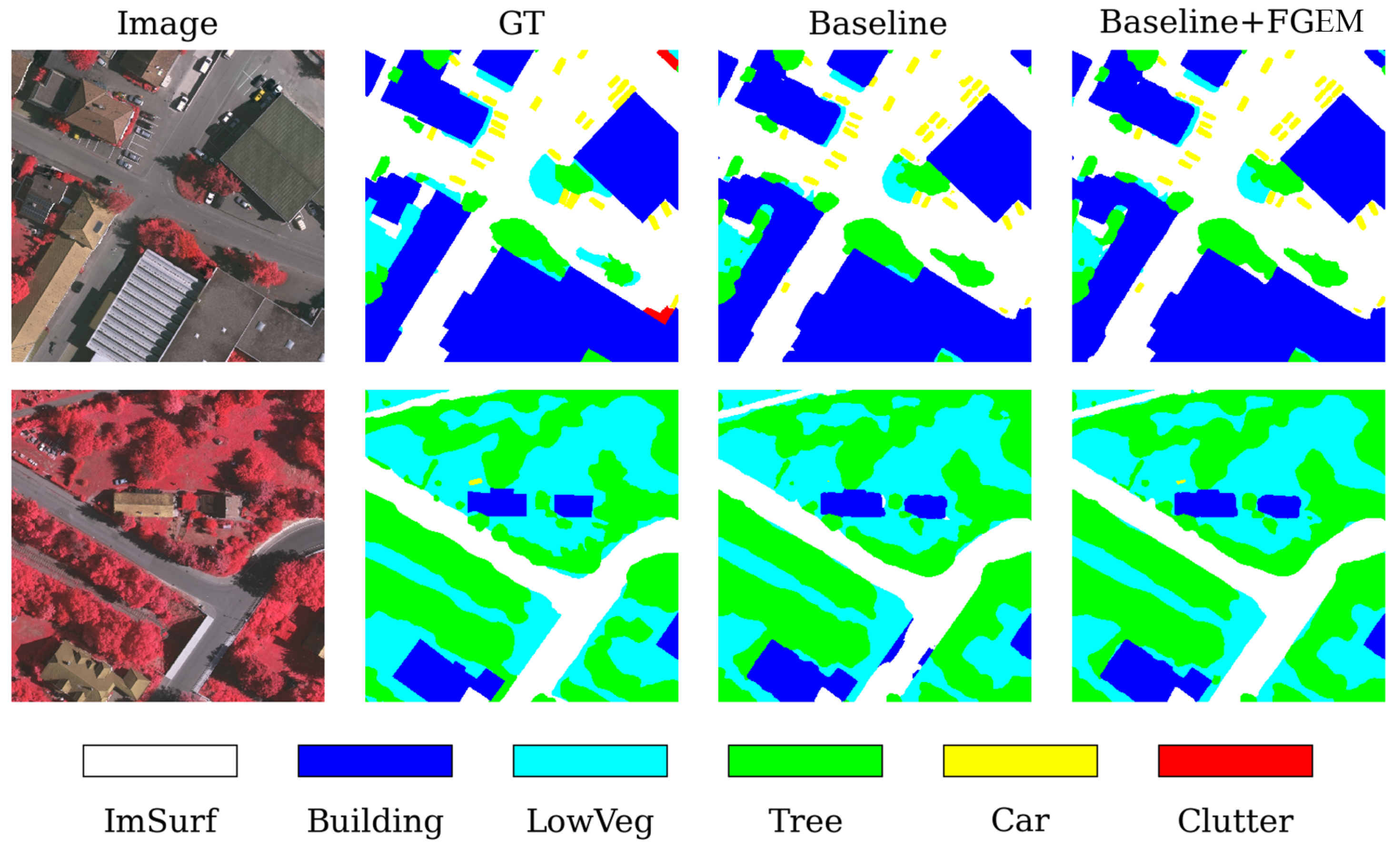
After introducing FGEM into the Baseline, mIoU and mF1 improve from 74.16% and 83.46% to 75.08% and 84.41%, respectively. These results indicate that frequency-guided feature enhancement effectively improves overall segmentation accuracy and category consistency. As shown in Figure 10, after introducing FGEM, the prediction results in complex background regions become more coherent, fragmentation is reduced, and discontinuities and noise near elongated structures are alleviated. In summary, FGEM mainly improves the robustness of the model in complex backgrounds and fine-grained structures by enhancing global structural representation and compensating for texture and detailed information, thereby yielding stable performance gains.

5.2.3. Influence of Local Category-Aware Frequency Attention Module

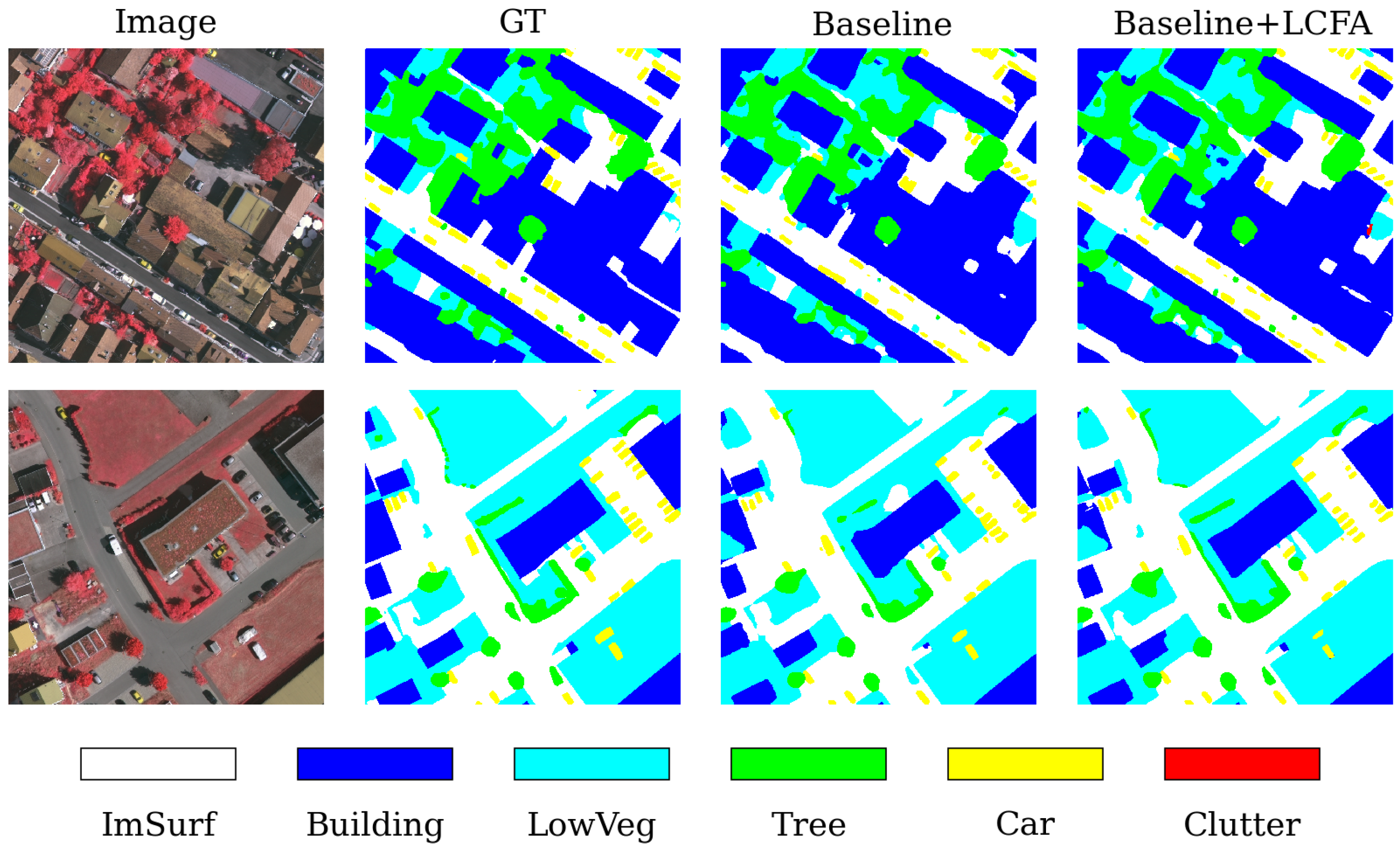
After introducing LCFA into the Baseline, mIoU increases from 74.16% to 75.11%, while mF1 and OA improve to 84.34% and 91.20%, respectively, indicating that local category-aware interaction enhances category discrimination capability during the decoding stage and yields stable performance gains. As shown in Figure 11, after introducing LCFA, the boundaries of structured objects such as buildings and roads become clearer, and the overflow phenomenon is reduced. Meanwhile, in regions with strong background interference, misclassification and adhesion phenomena are effectively suppressed. Overall, LCFA enhances the local detail recovery capability and category consistency of the model in complex regions by improving the fine-grained discrimination capability at boundaries and complex transition regions, and is one of the key modules driving the performance improvement.

5.2.4. Module-Removal Ablation Study

To verify the role of each module in the complete model, GCCM, FGEM, and LCFA are removed from the full model one by one, and the performance changes after removing each individual module are compared. The results show that removing any one of these modules leads to a decline in overall performance, with mIoU decreasing by 0.83%, 1.28%, and 2.04%, respectively, and mF1 decreasing by 0.61%, 1.02%, and 1.96%, respectively. These results indicate that GCCM, FGEM, and LCFA all play positive roles in improving the model performance.

As reported in

Table 6. Impact of different module removals on performance (%) on the ISPRS Vaihingen dataset. ↓ indicates the relative decrease compared with the full model.

Method	GCCM	FG	LCFA	mIoU (%)	mF1 (%)	OA (%)
w/o GCCM	×	✓	✓	76.07 (↓0.83)	85.25 (↓0.61)	91.32 (↓0.24)
w/o FGEM	✓	×	✓	75.62 (↓1.28)	84.84 (↓1.02)	91.51 (↓0.05)
w/o LCFA	✓	✓	×	74.86 (↓2.04)	83.90 (↓1.96)	91.29 (↓0.27)
Full	✓	✓	✓	76.90	85.86	91.56

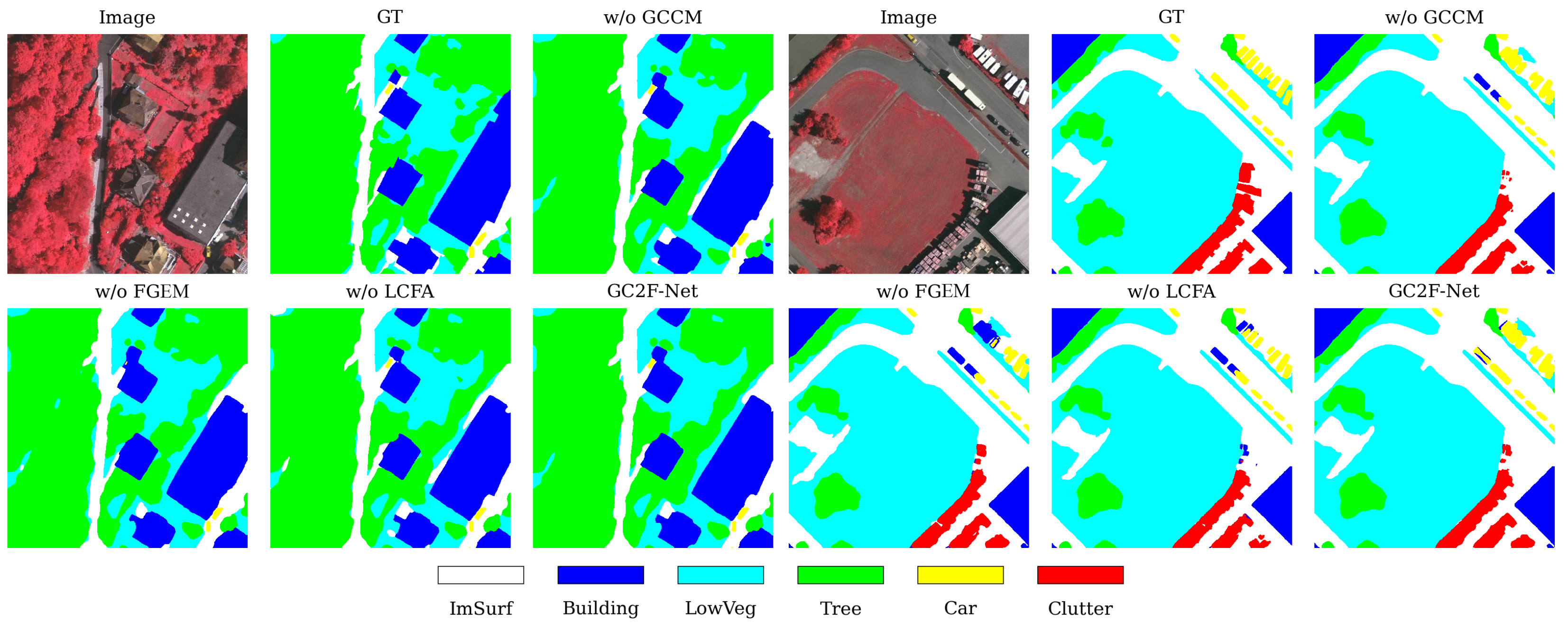
, removing GCCM, FGEM, or LCFA leads to performance degradation, demonstrating the effectiveness of each component. Figure 12 presents the qualitative comparison results. Without GCCM, the prediction results are more prone to block-wise misclassification caused by insufficient category consistency. After removing FGEM, the prediction stability in small-object and fine-grained structure regions decreases, and the noise and fragmentation become more pronounced. When LCFA is removed, boundary overflow and local adhesion are more likely to occur in category transition regions, thereby leading to incomplete target contours. In summary, GCCM, FGEM, and LCFA play complementary roles in category prior modeling, global structural representation enhancement, and fine-grained discrimination in boundaries and complex transition regions, respectively, jointly supporting the overall performance advantages of GC2F-Net.

In summary, the ablation experiments verify the effectiveness and complementarity of the key modules in GC2F-Net. Introducing GCCM, FGEM, or LCFA individually brings stable performance gains over the baseline framework, indicating that category prior modeling, frequency-domain enhancement, and local category-aware interaction each make independent contributions to performance improvement. Meanwhile, removing any of these modules from the complete model leads to performance degradation, demonstrating that all three are important components for improving segmentation performance. Overall, GCCM, FGEM, and LCFA collaboratively enhance category consistency, local detail recovery, and boundary discrimination from the perspectives of category-prior modeling, frequency-domain enhancement, and local category-aware interaction, respectively. This enables GC2F-Net to achieve more robust performance gains with only modest additional computational overhead.

6. Discussion

Systematic experiments conducted on the ISPRS Vaihingen, ISPRS Potsdam, and UAVid datasets validate the effectiveness and generalization ability of GC2F-Net for semantic segmentation in complex scenes. The advantages of GC2F-Net are mainly reflected in its improved overall evaluation metrics and its enhanced prediction quality for regions with complex textures, class boundaries, and fine-grained structures of small objects. On the Vaihingen and Potsdam datasets, GC2F-Net achieves superior results compared with existing methods in terms of mIoU, mF1, and OA. On the UAVid dataset, the proposed method also demonstrates strong scene adaptation capability, indicating favorable generalization performance under different imaging platforms, resolutions, and scene complexities.

To further discuss the robustness of GC2F-Net in practical remote sensing scenarios, we directly tested the same trained checkpoint on perturbed test images from the Vaihingen dataset. Two common visual perturbations were considered, including brightness variation and Gaussian blur, which simulate illumination changes and imaging blur that may occur during remote sensing image acquisition. As shown in

Table 7. Robustness evaluation of GC2F-Net under common visual perturbations on the Vaihingen dataset (%).

Condition	OA (%)	mF1 (%)	mIoU (%)	mIoU Drop (%)
Clean	91.56	85.86	76.90	–
Brightness variation	89.59	82.83	72.47	4.43
Gaussian blur	91.02	84.78	75.42	1.48

, GC2F-Net achieves an mIoU of 76.90% on the clean test set. Under brightness variation and Gaussian blur, the model maintains mIoUs of 72.47% and 75.42%, respectively, with corresponding mIoU drops of 4.43 and 1.48 percentage points. These results indicate that GC2F-Net maintains relatively stable segmentation performance under common visual perturbations, further supporting its robustness in complex remote sensing scenes.

Compared with conventional spatial-domain-based remote sensing semantic segmentation methods, the experimental results indicate that relying solely on spatial contextual modeling makes it difficult to simultaneously capture global structural representation and boundary detail recovery. By integrating frequency-domain information with spatial features, GC2F-Net enhances global structural representation while improving the discriminative capability of local details, thereby exhibiting more robust segmentation performance in regions with complex textures and category boundaries.

Although GC2F-Net achieves competitive overall performance, the category-level results indicate that it still has limitations in several challenging scenarios. On the Potsdam dataset, some categories, such as Tree and Car, do not always achieve the highest IoU among all comparison methods. For the Tree category, misclassification may occur between trees and low vegetation due to their similar spectral and texture distributions, especially around ambiguous boundary regions. For the Car category, omission or boundary deviation may still occur when vehicles are small, densely distributed, or partially occluded by shadows. On the UAVid dataset, the Human category remains particularly challenging because pedestrians usually occupy only a very small number of pixels and are easily affected by occlusion, scale variation, motion blur, and oblique-view imaging. In addition, cluttered urban backgrounds and fragmented object boundaries may still lead to local misclassification. These observations indicate that GC2F-Net still has room for improvement in extremely small-object recognition, ambiguous vegetation boundary delineation, and highly complex urban scenes.

In addition to the above category-level limitations, spatial-frequency collaborative modeling introduces additional feature transformation and fusion processes, which may increase model complexity and computational cost. Therefore, achieving a better balance between cross-domain information interaction, segmentation accuracy, and model efficiency remains an important challenge for future research.

In the future, more lightweight and efficient spatial-frequency collaborative modeling strategies will be explored to reduce model complexity while preserving the complementary advantages of spatial and frequency domains. Specifically, we will investigate lightweight frequency-aware modules, reduced-channel feature transformation, and dynamic feature interaction mechanisms to decrease parameters and FLOPs. In addition, multimodal information fusion will be further studied by incorporating complementary data sources, such as DSM and SAR, to improve the robustness of semantic segmentation in complex remote sensing scenes. Future research will also explore small-model-based collaborative frameworks and multi-agent systems, in which lightweight modules cooperate for spatial feature extraction, frequency-domain enhancement, and decision fusion, aiming to balance segmentation accuracy, efficiency, robustness, and practical deployment. For large-scale practical applications, overlap-based slicing and MapReduce-style parallel inference will also be investigated to reduce slicing-grid effects on small or thin objects while improving large-scale inference efficiency.

7. Conclusions

This paper proposes a spatial-frequency collaborative segmentation network for semantic segmentation of high-resolution remote sensing images. The GCCM, FGEM, and LCFA modules in GC2F-Net achieve collaborative modeling of global structural representations and local detail information through category prior fusion, frequency-domain feature enhancement, and local class-aware interaction, thereby improving the segmentation accuracy and robustness of the model in complex scenes. Experimental results demonstrate that GC2F-Net achieves robust and competitive segmentation performance on the ISPRS Vaihingen, ISPRS Potsdam, and UAVid datasets, with mIoU values of 76.90%, 79.44%, and 67.04%,indicating favorable generalization capability and application potential. Overall, the proposed method provides an effective modeling paradigm for semantic segmentation of high-resolution remote sensing images. Future work will explore lightweight models and multimodal information fusion to enhance the cross-scene generalization capability and segmentation performance.