Estimation of Soil Total Nitrogen in Plateau Agriculture Regions from UAV Hyperspectral Data

Highlights

What are the main findings?

• UAV hyperspectral imagery was successfully used to estimate soil total nitrogen (STN) in plateau agricultural areas.
• Multiple feature selection methods, including Pearson, VIP, CARS, and CARS-SPA, were compared to identify sensitive spectral bands.
• The VIP–PCA–SVR–RBF model achieved the best performance for STN prediction.
• Spatial distribution maps of STN revealed clear field-scale variability.

What are the implications of the main findings?

• UAV hyperspectral remote sensing combined with machine learning provides an effective approach for rapid STN estimation.
• The proposed method can support precision agriculture and field-scale soil nutrient management in plateau agricultural regions.

Abstract

Soil total nitrogen (STN) is a key indicator of soil fertility and plays a fundamental role in agricultural productivity and sustainable land management. However, achieving an accurate and spatially continuous estimate of STN at the field scale remains challenging due to inherent soil variability and the constraints of conventional sampling methods. In this study, we employed unmanned aerial vehicle (UAV)-based hyperspectral imagery to estimate STN by integrating spectral preprocessing, feature selection, and machine learning techniques. Multiple feature selection methods, including Pearson correlation analysis, variable importance in projection (VIP), and competitive adaptive reweighted sampling (CARS), were evaluated to identify the most informative spectral bands. Several regression models—support vector regression with radial basis function kernel (SVR-RBF), random forest (RF), Extra Trees, PCA-SVR-RBF, and XGBoost—were compared for STN prediction. Among these, the VIP-PCA-SVR-RBF model yielded the best performance, achieving a test R² of approximately 0.77 and an RMSE of 0.45 g kg⁻¹. The integration of VIP-based feature selection with PCA dimensionality reduction significantly enhanced predictive accuracy and generalization capability compared to the other models tested. Spatial prediction maps derived from the optimal model revealed considerable heterogeneity in STN distribution across the study area. These results underscore the potential of UAV hyperspectral remote sensing for high-resolution mapping of soil nitrogen and offer a promising framework for precision nutrient management in agriculture.

1. Introduction

Soil total nitrogen (STN) is a key indicator of soil fertility and is vital for regulating crop growth, ecosystem productivity, and agricultural sustainability [1]. Accurate data on soil nitrogen levels is crucial for optimizing fertilizer use, increasing crop yields, and minimizing environmental risks from excessive nitrogen application [2]. However, soil nitrogen often shows strong spatial variability in agricultural fields, which makes efficient monitoring techniques essential for sustainable land management [3].

Traditional methods for determining soil nitrogen mainly rely on laboratory-based chemical analysis techniques, such as the Kjeldahl method and elemental analysis [4]. Although these approaches provide accurate and reliable measurements, they are time-consuming, labor-intensive, and limited in spatial coverage, which restricts their application in large-scale soil monitoring [5]. Therefore, developing rapid, non-destructive, and spatially continuous techniques for soil nitrogen estimation has become an important research focus in soil science and environmental monitoring [2,6]. Remote sensing techniques provide an alternative approach for large-scale soil property monitoring. Early studies mainly relied on multispectral remote sensing data to estimate soil characteristics such as organic matter and nitrogen content [7]. However, multispectral sensors provide only a limited number of spectral bands, which restricts their ability to detect subtle biochemical variations in soils. Compared with multispectral data, hyperspectral remote sensing provides hundreds of narrow and contiguous spectral bands and continuous spectral information, which significantly improves the capability for detecting soil biochemical properties [8,9]. Numerous studies have demonstrated strong relationships between soil nitrogen content and spectral reflectance in the visible and near-infrared regions, which are often associated with organic matter absorption features and indirect nitrogen-related spectral responses [5,6]. Therefore, hyperspectral remote sensing has shown great potential for quantitative estimation of soil properties [8].

With the rapid development of unmanned aerial vehicle (UAV) technology, UAV-based hyperspectral remote sensing has emerged as an effective tool for high-resolution soil monitoring [10]. Compared with satellite platforms, UAV hyperspectral systems provide higher spatial resolution, flexible acquisition timing, and reduced atmospheric interference, making them particularly suitable for monitoring heterogeneous agricultural landscapes. These advantages enable UAV hyperspectral imagery to capture fine-scale spatial variability of soil properties within agricultural fields. Recent studies have demonstrated the effectiveness of UAV hyperspectral data for agricultural and soil applications. For example, hyperspectral imaging systems mounted on UAV platforms have been widely applied in crop monitoring, vegetation parameter retrieval, and soil property estimation [10,11,12]. These studies indicate that UAV hyperspectral technology provides new opportunities for high-resolution mapping of soil nutrients and supports the development of precision agriculture.

However, hyperspectral datasets are typically characterized by high dimensionality and significant spectral redundancy, which can decrease model stability and prediction accuracy if not properly managed [13]. Therefore, feature selection techniques have become crucial for identifying informative wavelengths and reducing redundant spectral information. Previous studies have successfully applied different feature selection algorithms for soil property estimation [14]. For example, Lin et al. [15] applied hyperspectral reflectance and PLSR to estimate soil total nitrogen in a coal-mining subsidence area of China and achieved reliable prediction accuracy. Datta et al. [16] further used hyperspectral datasets from agricultural soils in Germany and Sweden with machine learning models and confirmed the effectiveness of hyperspectral data for predicting soil nitrogen. In addition, hyperspectral spectroscopy combined with regression modeling has also been successfully applied to estimate soil total nitrogen in orchard soils of Yantai, China [17]. Techniques such as Pearson correlation analysis, variable importance in projection (VIP), and competitive adaptive reweighted sampling (CARS) are widely used in hyperspectral soil studies. Additionally, machine learning algorithms including support vector machines (SVMs), random forest (RF), and gradient boosting models have demonstrated strong ability in capturing nonlinear relationships between hyperspectral reflectance and soil properties [18]. Therefore, integrating effective feature selection methods with machine learning models has become a key strategy for improving soil property estimation based on hyperspectral data.

In this study, UAV hyperspectral imagery was used to estimate soil total nitrogen (STN) in agricultural fields of a plateau region. While previous studies have explored various feature selection methods and machine learning models for hyperspectral inversion, most of them focus on individual methods or simple model comparisons, and the combined effects of feature selection, dimensionality reduction, and model stability under limited sample conditions have not been sufficiently addressed. In particular, the robustness of model performance with respect to data partitioning remains insufficiently investigated.

To address these gaps, this study develops and evaluates an integrated framework for STN estimation that combines feature selection, dimensionality reduction, and machine learning methods. Specifically, a combined VIP–PCA–SVR–RBF approach is adopted to reduce spectral redundancy, mitigate multicollinearity, and improve model stability and generalization performance. In addition, multiple feature selection methods and regression models are systematically compared, and additional repeated random-split analysis is included to support the examination of model performance variability under different data partitions.

The results of this study not only provide high-resolution spatial mapping of STN at the field scale, but also offer insights into the reliability and limitations of hyperspectral inversion models under practical agricultural conditions. These findings contribute to a more realistic evaluation of model applicability and provide useful insights for future hyperspectral-based soil nutrient monitoring and model development.

The remainder of this paper is organized as follows. Section 2 describes the study area, soil sampling and laboratory analysis, UAV hyperspectral data acquisition and preprocessing, and the methods for feature band selection and model construction. Section 3 presents the results of model performance comparison and the spatial prediction of soil total nitrogen. Section 4 discusses the performance, uncertainties, and limitations of the proposed approach. Finally, Section 5 summarizes the main conclusions of this study.

2. Materials and Methods

2.1. Study Area

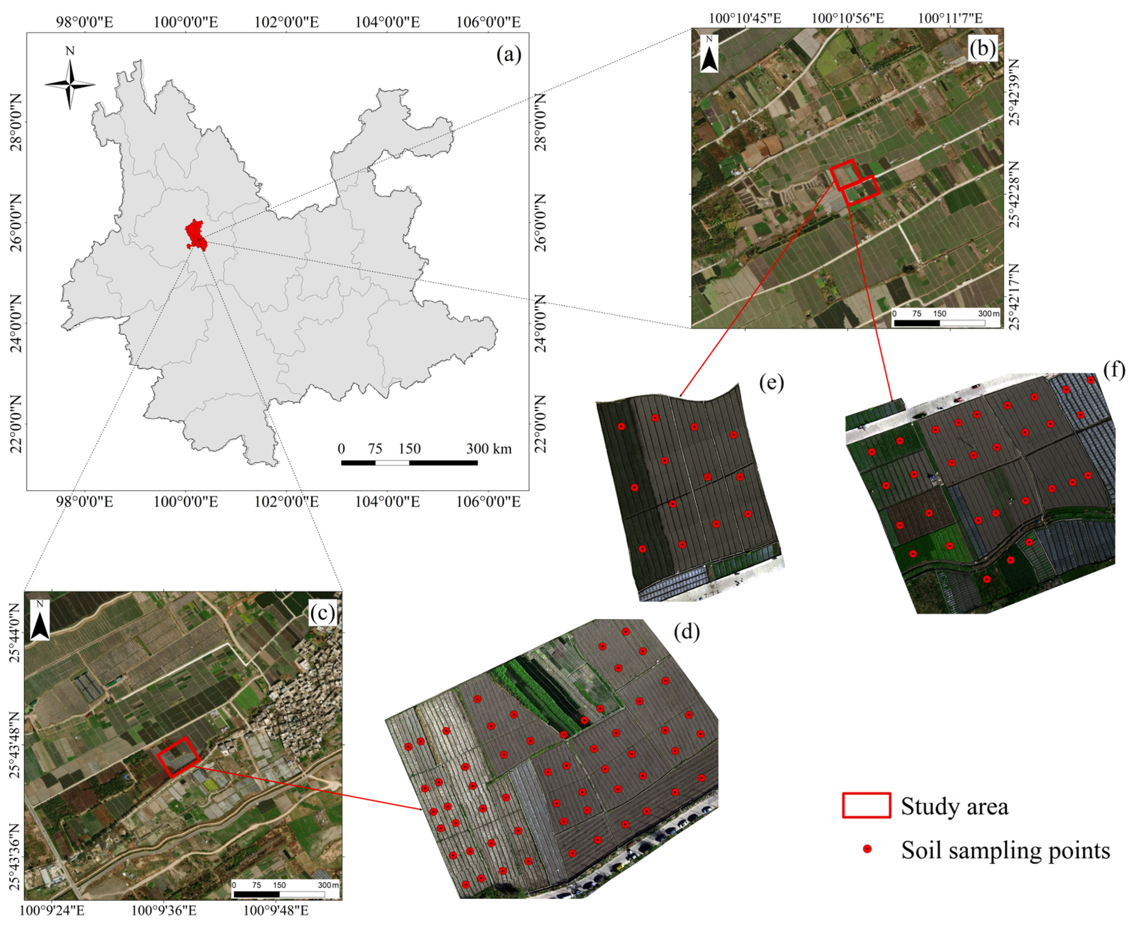
The study area is located in Dali City, Yunnan Province, in southwestern China, within a typical low-latitude plateau agricultural region. Soil sampling was carried out in Xiaoyizhuang Village (25°42′N, 100°10′E) and Majiuyi Village (25°43′N, 100°09′E), as shown in Figure 1. The area sits on the Yunnan–Guizhou Plateau and features gently rolling terrain with elevations between approximately 1900 and 2100 m above sea level. It has a low-latitude plateau monsoon climate characterized by distinct dry and wet seasons, an average annual temperature of about 15 °C, and yearly precipitation averaging around 1000 mm. The landscape is dominated by agricultural land, where intensive farming practices are common, and primary crops include vegetables and maize grown in seasonal rotation systems. According to the Chinese Soil Taxonomy, the main soil types are red soil, yellow-brown soil, and paddy soil [19], and variations in topography and farming methods lead to significant spatial differences in soil properties [3].

2.2. Soil Sampling and Analysis

Soil sampling was carried out from 25 to 27 March 2024, under clear weather conditions. At each sampling site, a composite soil sample was collected using a three-point sampling method [1], where three subsamples were taken within a small area and thoroughly mixed to minimize microscale spatial heterogeneity. Surface soil samples (0–20 cm) were obtained after removing visible plant residues, weeds, and stones, and the surrounding surface conditions and geographic coordinates of each site were documented. Minor adjustments to sampling locations were made to account for field accessibility and local circumstances.

In total, 100 valid soil samples were collected across the study area, including samples from both bare-soil fields and vegetable cultivation zones. UAV hyperspectral imagery was captured simultaneously with soil sampling. After collection, approximately 500 g of each composite sample was sealed in plastic bags and transported to the laboratory. The samples were air-dried at room temperature, ground, and sieved to ≤0.25 mm before analysis. Soil total nitrogen (STN) content was measured using the automated Kjeldahl method [4], following the agricultural industry standard NY/T 1121.24–2012 [20], with STN values expressed in g kg⁻¹.

For the modeling analysis, only the bare-soil samples were used in order to avoid spectral interference caused by vegetation cover. A total of 82 bare-soil samples were selected, among which 57 samples were assigned to the training set and 25 samples to the test set.

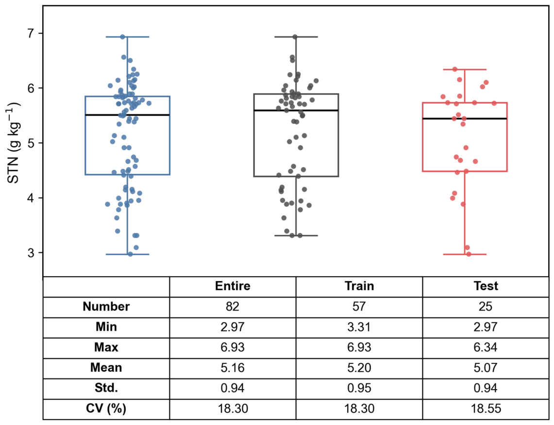
The descriptive statistics of STN for the entire dataset and the training and test subsets are shown in Figure 2. For the entire dataset, STN values ranged from 2.97 to 6.93 g kg⁻¹, with a mean value of 5.16 g kg⁻¹ and a standard deviation of 0.94 g kg⁻¹. The coefficient of variation (CV) was 18.30%, indicating a moderate level of spatial variability in soil nitrogen content within the study area. For the training dataset, STN values ranged from 3.31 to 6.93 g kg⁻¹, with a mean value of 5.20 g kg⁻¹. The test dataset showed a similar range of 2.97–6.34 g kg⁻¹ and a mean value of 5.07 g kg⁻¹. The statistical characteristics of the training and test datasets were generally consistent with those of the entire dataset, indicating that the dataset partitioning was reasonable and suitable for subsequent model development and testing.

2.3. UAV Hyperspectral Data Acquisition and Preprocessing

UAV hyperspectral data were collected using a DJI Matrice 350 RTK platform (DJI, Shenzhen, China) equipped with a FigSpec FS-60C hyperspectral imaging system (FigSpec, Hangzhou, China). The main parameters of the UAV hyperspectral sensor are summarized in

Table 1. Main parameters of the UAV hyperspectral imaging system.

Parameters	Value	Parameters	Value
UAV platform	DJI Matrice 350 RTK	Spectral range	400–1000 nm
Hyperspectral sensor	FigSpec FS-60C	Spectral resolution	<2.5 nm
Detector	CMOS	Spectral bands	300
Flight altitude	80 m	Side overlap	70%

. The sensor covers a spectral range of 400–1000 nm with a spectral resolution of better than 2.5 nm. Data collection took place from 25 to 27 March 2024, under clear weather conditions. Before each flight, a white reference calibration was performed using a standard white panel to aid in reflectance correction [11]. Flight missions were carried out at an altitude of 80 m to capture hyperspectral strip imagery over the study area, with the side overlap between adjacent flight lines set to 70% to ensure sufficient coverage for subsequent mosaicking.

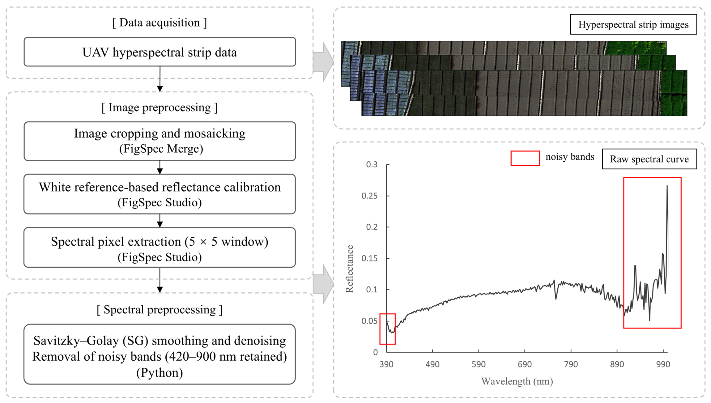
The acquired hyperspectral strip data were first cropped and mosaicked using FigSpec Merge software (FigSpec, Hangzhou, China), which produced preliminary hyperspectral images. The mosaicked images were then imported into FigSpec Studio 2.0 (FigSpec, Hangzhou, China), where additional cropping and reflectance calibration were performed based on a ground white reference panel. These steps converted the original imagery into surface reflectance data. To extract representative spectral information for soil sampling sites, a 5 × 5 pixel window centered on each sampling point was defined [8], and the mean reflectance within the window was calculated to reduce random noise associated with single-pixel extraction.

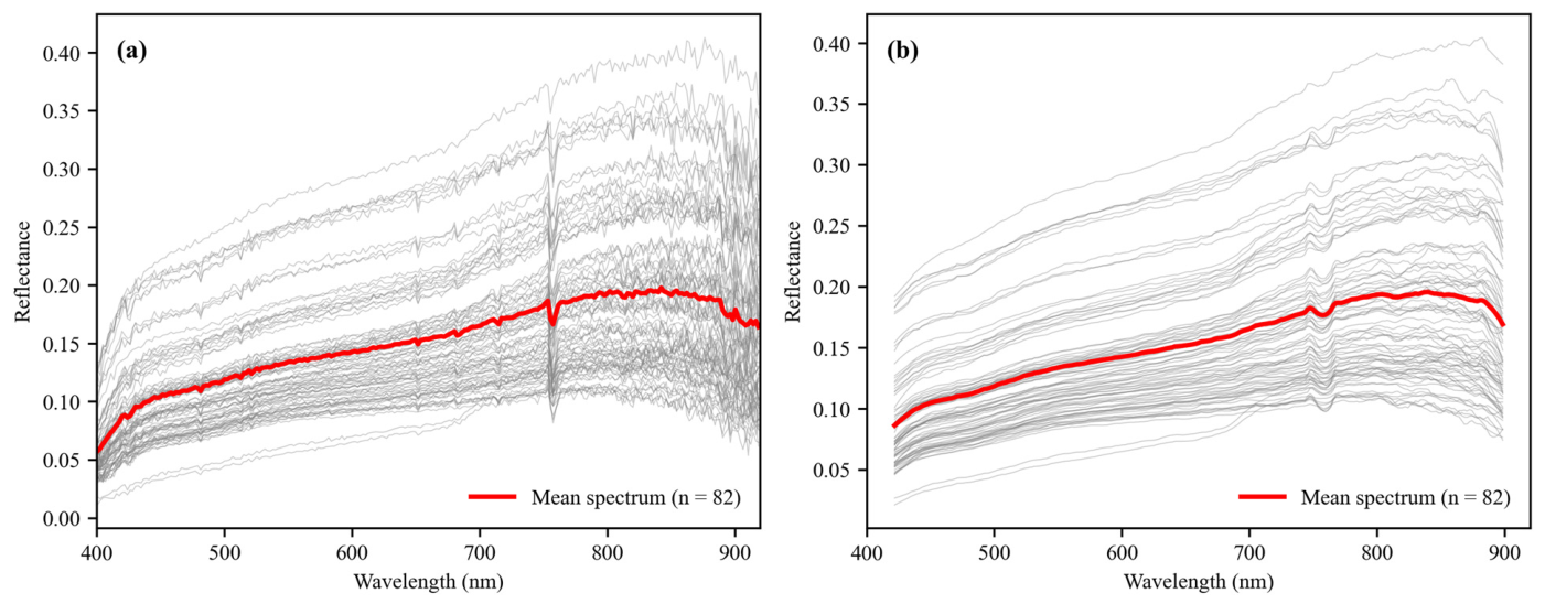
All spectral data were resampled to a uniform wavelength interval of approximately 2.15 nm. Savitzky–Golay (SG) filtering was then applied to smooth the spectral curves [21], using a window size of 11 and a polynomial order of 2 to reduce noise while preserving spectral features. Noisy bands at both spectral ends were removed, and a total of 233 bands within the wavelength range of 420–900 nm were retained for subsequent analysis. To visually demonstrate the smoothing effect of SG preprocessing, the raw and SG-smoothed bare-soil spectra are compared in Figure 3. The raw spectra exhibit noticeable noise and fluctuations, particularly near the spectral edges, whereas the SG-smoothed spectra are smoother while retaining the overall spectral profile.

The overall preprocessing workflow, including image cropping and mosaicking, reflectance calibration, spectral extraction, SG smoothing, and noisy-band removal, is illustrated in Figure 4.

2.4. Feature Selection and Modeling Methods

2.4.1. Feature Band Selection

UAV hyperspectral data typically contain hundreds of contiguous spectral bands, which often exhibit strong redundancy and multicollinearity. When combined with a limited number of ground samples, this high dimensionality may lead to unstable model performance and overfitting [22]. Therefore, feature band selection was performed before model construction to reduce spectral redundancy and improve the robustness of soil total nitrogen (STN) prediction.

Pearson correlation analysis was first applied as a filter-based method to quantify the linear relationship between spectral reflectance and measured STN [23]. The Pearson correlation coefficient $r$ was calculated as:

$$r={\displaystyle \frac{{\sum }_{i=1}^n\left(x_i-\overline{x}\right)\left(y_i-\overline{y}\right)}{\sqrt{{\sum }_{i=1}^n{\left(x_i-\overline{x}\right)}^2}\sqrt{{\sum }_{i=1}^n{\left(y_i-\overline{y}\right)}^2}}}$$

(1)

where $x_i$ represents spectral reflectance at a given wavelength, $y_i$ denotes the corresponding STN value, and $n$ is the number of samples. Bands with higher absolute correlation coefficients were considered to be more sensitive to STN.

Variable Importance in Projection (VIP), derived from partial least squares regression (PLSR) [24], was employed to evaluate the contribution of each spectral band to STN prediction while accounting for the covariance structure of spectral variables [25]. The VIP score for the $j$-th band is defined as:

$${VIP}_j=\sqrt{p·{\displaystyle \frac{{\sum }_{k=1}^A{SSY}_k·{\omega }_{jk}^2}{{\sum }_{k=1}^A{SSY}_k}}}$$

(2)

where $p$ denotes the total number of spectral bands, $A$ is the number of latent variables in the PLSR model, ${SSY}_k$ represents the explained variance of the response variable by the $k$-th latent variable, and ${\omega }_{jk}$ is the weight of the $j$-th band in the $k$-th latent variable. Bands with $VIP>1$ were considered important contributors.

In addition, Competitive Adaptive Reweighted Sampling (CARS) was adopted as a model-based variable selection method [14]. CARS iteratively selects informative wavelengths based on the stability of regression coefficients during Monte Carlo sampling, progressively eliminating less relevant variables. To further minimize collinearity among selected bands, the successive projections algorithm (SPA) was applied following CARS (CARS-SPA) [26], resulting in a compact and minimally redundant feature subset. All feature selection methods were conducted on Savitzky–Golay (SG) smoothed reflectance spectra within the 420–900 nm range [21].

The feature selection results obtained using different methods are summarized in

Table 2. Selected wavelength bands obtained using different feature selection methods.

Method	Number of Bands	Selected Wavelengths (nm)
Pearson correlation	30	802, 804, 836, 838, 840, 842, 844, 846, 848, 850,852, 854, 856, 858, 860, 862, 864, 866, 868, 870,872, 874, 876, 878, 880, 882, 884, 886, 888, 890
VIP	65	422, 424, 426, 428, 430, 432, 434, 436, 438, 441, 443, 445, 447, 449, 452, 454, 456, 458, 460, 462, 464, 466, 468, 471, 473, 475, 477, 479, 481, 483, 485, 488, 490, 492, 494, 496, 557, 559, 561, 563, 565, 567, 569, 826, 850, 852, 858, 860, 862, 866, 868, 870, 872, 876, 878, 880, 882, 884, 886, 888, 890, 892, 894, 896, 898
CARS	15	466, 488, 490, 548, 557, 567, 569, 571, 573, 647, 672, 826, 846, 852, 886
CARS-SPA	12	432, 454, 481, 492, 553, 573, 656, 672, 686, 756, 784, 842

Note: Pearson, VIP, CARS, and CARS–SPA denote Pearson correlation, variable importance in projection, competitive adaptive reweighted sampling, and the combination of CARS with the successive projections algorithm, respectively.

. Pearson correlation analysis selected 30 bands, mainly concentrated in the near-infrared region between 802 and 890 nm, indicating relatively strong linear relationships between STN and reflectance in this wavelength range [23]. The VIP method retained 65 bands, covering a broader spectral range including the visible region (422–496 nm) [24], a narrow interval around 557–569 nm, and the near-infrared region (826–898 nm), suggesting that VIP preserved more informative variables related to STN prediction. The CARS algorithm further reduced the feature set to 15 bands distributed across several discrete spectral regions in both the visible and near-infrared ranges [14]. After applying SPA to the CARS-selected bands, the CARS–SPA method produced a more compact subset of 12 bands, which were sparsely distributed across the spectrum and exhibited lower redundancy [25]. These selected feature subsets were subsequently used as inputs for model construction and performance comparison.

Beyond the differences in the number of selected bands, the distribution of selected wavelengths across different feature selection methods exhibited a certain degree of consistency. Most characteristic bands were concentrated in the visible and near-infrared regions, particularly within the ranges of approximately 420–460 nm, 550–570 nm, 650–700 nm, and 780–900 nm. These spectral regions are closely associated with soil reflectance properties and have been widely reported to be sensitive to variations in soil nitrogen content.

Although different methods (e.g., Pearson correlation, VIP, CARS, and CARS-SPA) selected different specific bands, they generally captured similar spectral regions, indicating that these wavelength ranges contain important information for STN estimation. This consistency enhances the reliability of the selected features and provides useful guidance for future hyperspectral studies on soil nitrogen inversion.

2.4.2. Model Construction

Based on the selected spectral feature subsets, several machine-learning regression models were developed to estimate soil total nitrogen (STN). The models included support vector regression with a radial basis function kernel (SVR-RBF) [27], Random Forest (RF) [28], Extremely Randomized Trees (Extra Trees) [29], and Extreme Gradient Boosting (XGBoost) were implemented to model the relationship between hyperspectral reflectance and STN [30], which are widely used in hyperspectral regression tasks.

SVR has been widely used in hyperspectral regression tasks due to its strong generalization ability and effectiveness in handling nonlinear relationships in high-dimensional datasets [31,32]. The radial basis function (RBF) kernel allows SVR to map input data into a higher-dimensional feature space, enabling the model to capture complex nonlinear patterns between spectral variables and soil properties. Random Forest and Extra Trees are ensemble learning algorithms based on decision trees that construct multiple decision trees during training and aggregate their predictions to improve model stability and predictive performance [28,29]. These tree-based ensemble models are particularly effective in handling high-dimensional data and are robust to noise and overfitting. XGBoost is a gradient-boosting framework that builds additive prediction models by sequentially combining weak learners and has demonstrated high predictive accuracy and computational efficiency in many remote sensing and environmental modeling applications [30].

Although feature selection methods (e.g., Pearson correlation, VIP, CARS, and CARS-SPA) effectively reduced spectral redundancy and identified informative wavelengths, the selected bands—especially adjacent wavelengths—may still exhibit substantial multicollinearity. To address this issue, principal component analysis (PCA) was applied before SVR to construct a PCA-SVR-RBF model, aiming to further reduce spectral dimensionality and alleviate multicollinearity among spectral variables [33]. In the PCA-SVR-RBF framework, the number of retained principal components was treated as a tunable parameter and optimized using grid search within the training dataset. The PCA transformation was fitted using the training dataset and then applied to the test dataset to avoid potential data leakage. The cumulative explained variance of the retained principal components was recorded for each feature scheme to ensure that the transformed variables preserved most of the spectral information [34]. While PCA effectively reduces multicollinearity and dimensionality, it may reduce the direct interpretability of the transformed spectral variables.

To ensure reproducibility and fair comparison among models, the hyperparameters were explicitly defined and optimized. For the SVR model with a radial basis function (RBF) kernel, the penalty coefficient (C), kernel parameter (γ), and epsilon (ε) were optimized using a grid search strategy with five-fold cross-validation. For the Random Forest (RF) and Extra Trees models, the number of trees, maximum depth, minimum samples per leaf, and maximum features were tuned to achieve optimal performance. Similarly, for the XGBoost model, the key hyperparameters, including the number of trees, maximum depth, learning rate, subsample ratio, column sampling ratio, minimum child weight, and regularization coefficient, were optimized using grid search. All hyperparameter tuning procedures were conducted exclusively on the training dataset to avoid information leakage, and the final model performance was evaluated using an independent test set. Compared with models using VIP-selected variables alone, the PCA-SVR-RBF framework was expected to improve prediction stability and generalization performance.

2.4.3. Model Accuracy Assessment

The dataset was randomly divided into training and test subsets at a ratio of 7:3 using a fixed random seed (seed = 42) to ensure reproducibility. Given that the samples were collected from multiple field plots within the study area, this random partitioning strategy may not fully account for potential spatial autocorrelation among neighboring samples. Nevertheless, it provides a straightforward and widely used approach for model evaluation at the field scale. Model performance was evaluated using both the training and test datasets.

The coefficient of determination (R²) is defined as:

$$R^2=1-{\displaystyle \frac{{\sum }_{i=1}^n{\left(y_i-\widehat{y_i}\right)}^2}{{\sum }_{i=1}^n{\left(y_i-\overline{y}\right)}^2}}$$

(3)

The root mean square error (RMSE) is calculated as:

$$RMSE=\sqrt{{\displaystyle \frac{1}{n}}{\displaystyle \sum _{i=1}^n}{\left(y_i-{\widehat{y}}_i\right)}^2}$$

(4)

The residual prediction deviation (RPD) is defined as [5]:

$$RPD={\displaystyle \frac{SD}{RMSE}}$$

(5)

where $y_i$ and $\widehat{y_i}$ represent the measured and predicted STN values, respectively; $\overline{y}$ is the mean of measured values; $n$ is the number of samples; and $SD$ denotes the standard deviation of measured STN values.

3. Results

3.1. Mapping of Soil Total Nitrogen

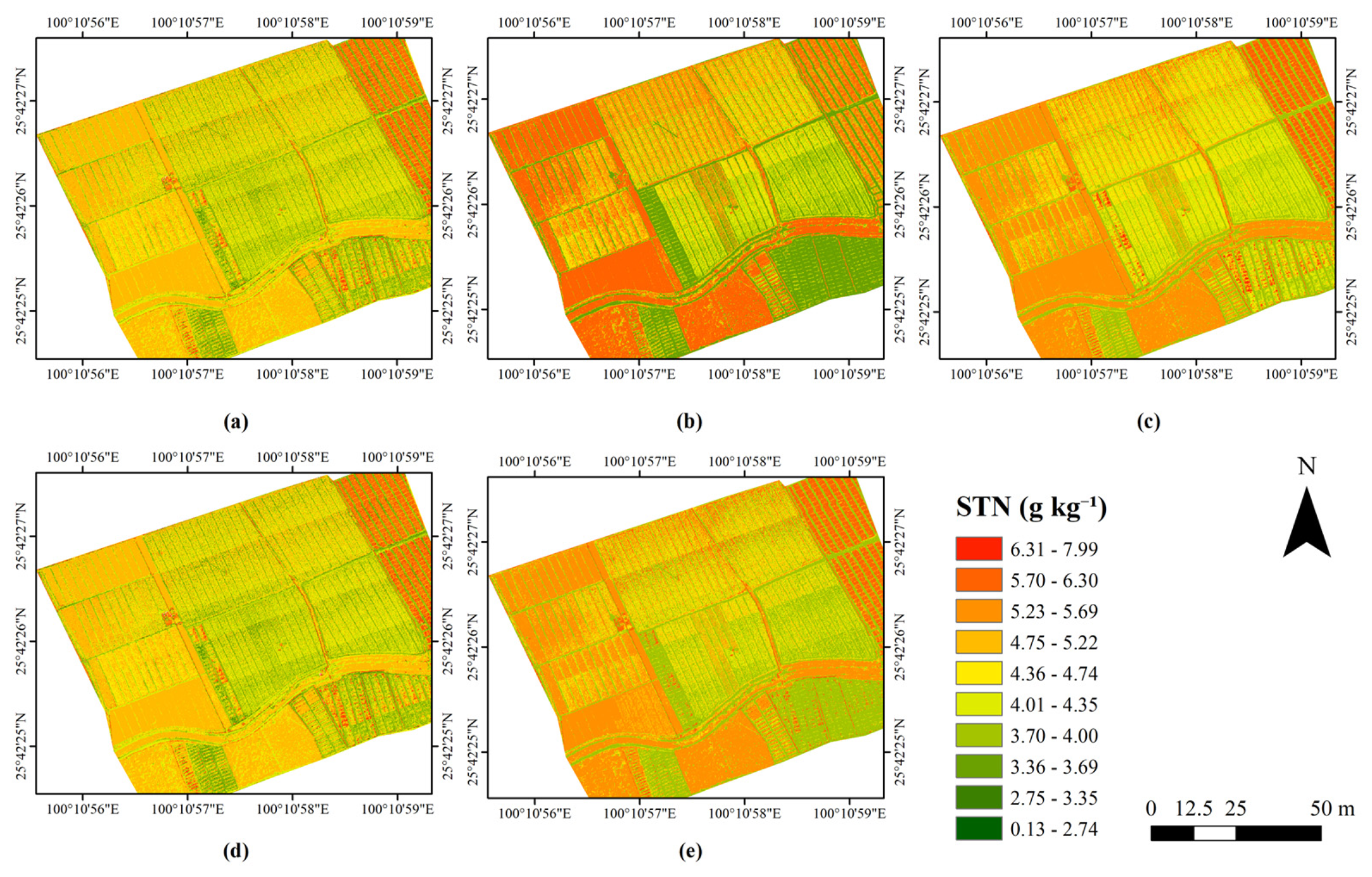
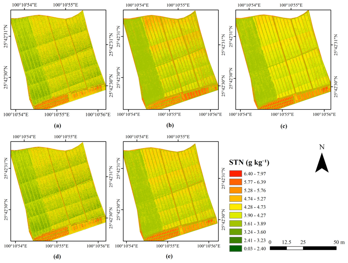
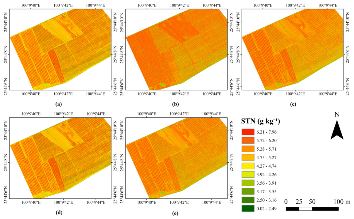
Using the optimal feature–model combination (VIP-PCA-SVR-RBF), the spatial distribution of soil total nitrogen (STN) was predicted for the UAV survey areas. The predicted STN distribution maps generated by different regression models are presented in Figure 5, Figure 6 and Figure 7, illustrating the spatial distribution patterns of soil nitrogen at the field scale.

In Field A of Xiaoyizhuang Village (Figure 5), the predicted STN values are mainly distributed within a moderate range, with most areas appearing in yellow to light-green tones, corresponding to STN levels of approximately 3.9–5.3 g kg⁻¹. However, relatively higher STN values can still be observed in several localized areas, which may be related to differences in surface conditions. In contrast, the large bare-soil regions exhibit relatively stable STN levels with smoother spatial variations.

In Field B of Xiaoyizhuang Village (Figure 6), the spatial distribution of STN shows more noticeable variations compared with Field A. Most of the central cultivated areas are dominated by moderate STN levels, mainly represented by yellow and light-green colors. In contrast, relatively lower STN values appear in several marginal areas, while higher STN values are observed in some northern parts of the field. These spatial variations may reflect differences in surface conditions across the field.

In the Majiuyi field (Figure 7), the predicted STN values are generally higher than those in the previous two fields, with most areas dominated by orange to yellow tones, corresponding to moderate to relatively high STN levels (4.7–6.3 g kg⁻¹). The spatial distribution of STN in this field appears relatively uniform, suggesting more consistent soil fertility conditions across the cultivated area. Only a few localized patches with relatively lower STN values can be observed.

Although slight differences exist among the regression models in terms of local spatial textures, the overall spatial patterns remain highly consistent across the five models. Pearson–RF and CARS–XGBoost tend to produce stronger local contrasts, whereas the VIP–PCA–SVR-RBF model generates smoother spatial transitions while preserving the main spatial structures of the fields. These results demonstrate that UAV hyperspectral data combined with machine learning models can effectively capture the fine-scale spatial variability of soil nitrogen in agricultural landscapes.

3.2. Inter-Comparison of Different Models

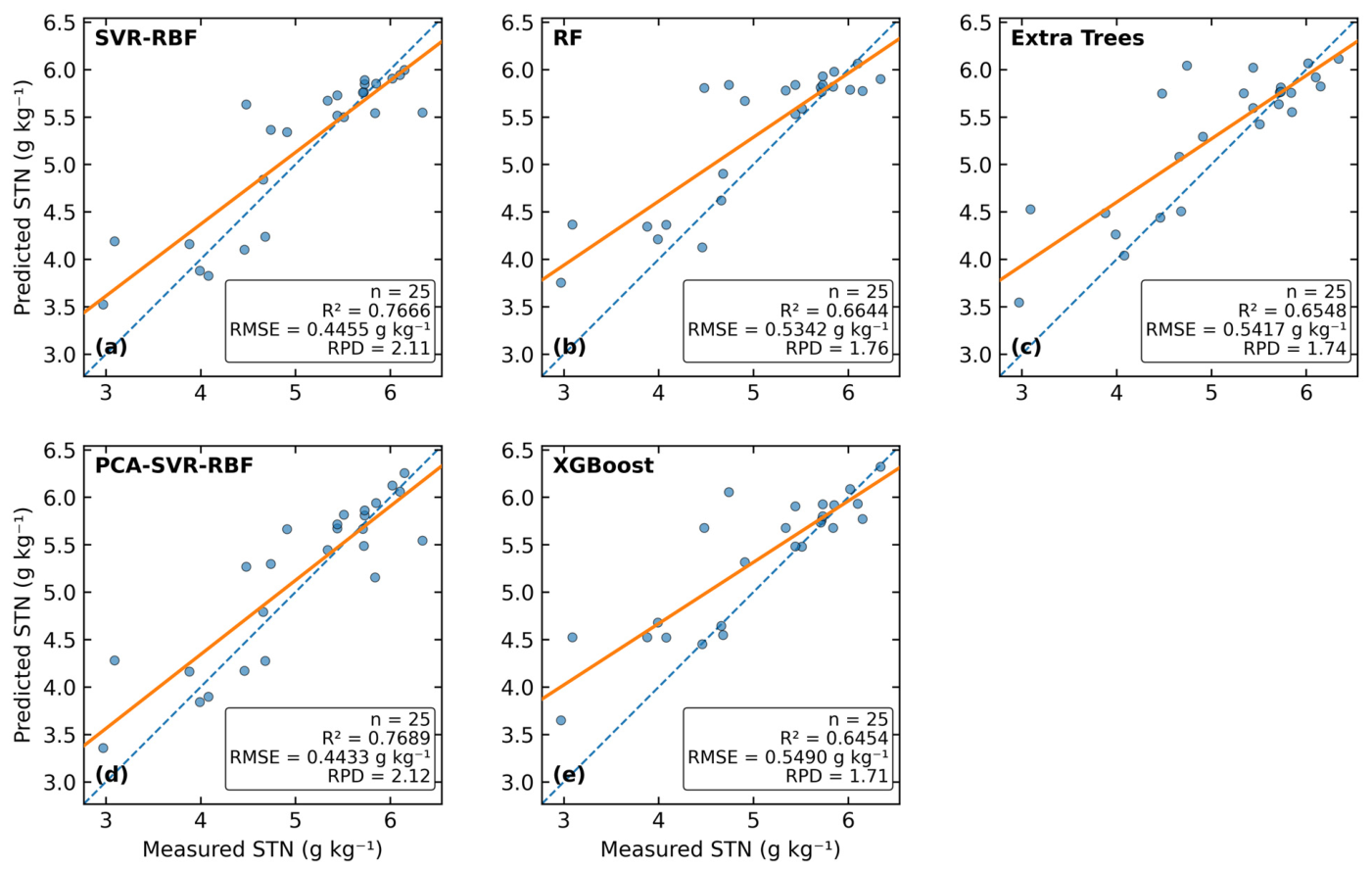
A comparative analysis of different regression models under multiple feature selection schemes was conducted in this study. The predictive performance of these models was evaluated using the independent test dataset. Model accuracy was assessed using the coefficient of determination (R²), root mean square error (RMSE), and residual prediction deviation (RPD) [5]. The quantitative evaluation results are summarized in

Table 3. Performance comparison of regression models for soil total nitrogen (STN) prediction using different feature selection methods.

Model	Feature Scheme	Training Set			Test Set
		R2	RMSE (g kg−1)	RPD	R2	RMSE (g kg−1)	RPD
SVR-RBF	Full-band	0.9872	0.1068	8.914	0.6700	0.5297	1.777
	Pearson	0.6254	0.5776	1.649	0.6525	0.5436	1.731
	VIP	0.9374	0.2361	4.032	0.7666	0.4455	2.113
	CARS	0.8289	0.3904	2.439	0.7249	0.4836	1.946
	CARS-SPA	0.8031	0.4188	2.274	0.6625	0.5357	1.757
RF	Full-band	0.9531	0.2045	4.657	0.6446	0.5497	1.712
	Pearson	0.7704	0.4522	2.106	0.6644	0.5342	1.762
	VIP	0.9538	0.2029	4.692	0.6422	0.5515	1.706
	CARS	0.9631	0.1812	5.255	0.5983	0.5844	1.610
	CARS-SPA	0.9565	0.1969	4.835	0.6263	0.5637	1.670
Extra Trees	Full-band	0.9989	0.0312	30.525	0.5833	0.5952	1.581
	Pearson	0.6998	0.5170	1.842	0.6530	0.5431	1.733
	VIP	0.9989	0.0307	31.028	0.6548	0.5417	1.737
	CARS	0.9992	0.0266	35.814	0.6412	0.5523	1.704
	CARS-SPA	1.0000	0.0003	>10	0.6395	0.5537	1.700
PCA-SVR-RBF	Full-band	0.9860	0.1118	8.514	0.6691	0.5304	1.774
	Pearson	0.6253	0.5776	1.648	0.6526	0.5435	1.732
	VIP	0.9109	0.2817	3.379	0.7689	0.4433	2.123
	CARS	0.8289	0.3904	2.439	0.7251	0.4835	1.946
	CARS-SPA	0.8031	0.4188	2.274	0.6625	0.5357	1.757
XGBoost	Full-band	0.9888	0.0999	9.533	0.5742	0.6017	1.564
	Pearson	0.9194	0.2679	3.554	0.6148	0.5722	1.645
	VIP	0.9562	0.1975	4.821	0.5841	0.5947	1.583
	CARS	0.9924	0.0822	11.589	0.6454	0.5490	1.714
	CARS-SPA	0.9628	0.1820	5.231	0.5330	0.6301	1.494

Note: R², RMSE, and RPD denote the coefficient of determination, root mean square error, and residual prediction deviation, respectively. All models were evaluated using the same training–test split. Bold values indicate the best test performance for each regression model.

, while the agreement between measured and predicted STN values is illustrated in Figure 8.

Overall, the predictive performance of the models varied considerably across different feature selection schemes. When all spectral bands were used as input variables, several models exhibited relatively limited predictive ability, indicating that redundant information in the full-band hyperspectral data may negatively affect model performance. After applying feature selection methods, the prediction accuracy of most models improved, demonstrating the importance of dimensionality reduction in hyperspectral modeling [22].

Among the evaluated models, the PCA-SVR-RBF model combined with VIP-selected bands achieved the best predictive performance on the test dataset, with an R² of 0.7689, RMSE of 0.4433 g kg⁻¹, and RPD of 2.123. This result suggests that the integration of VIP-based feature selection and principal component analysis effectively extracts informative spectral variables while reducing multicollinearity among bands.

The SVR-RBF model with VIP-selected bands also showed strong predictive capability, achieving an R² of 0.7666 and RMSE of 0.4455 g kg⁻¹ on the test dataset. In contrast, the tree-based models (RF and Extra Trees) demonstrated relatively stable performance across different feature schemes but did not outperform the PCA-SVR-RBF model in terms of prediction accuracy. The XGBoost model, although benefiting from feature selection, showed comparatively lower predictive performance.

The scatter plots in Figure 8 further illustrate the relationships between measured and predicted STN values for the best configuration of each regression model. Compared with the other models, the PCA-SVR-RBF model shows predictions more closely distributed around the 1:1 line, indicating better agreement between predicted and measured values.

Overall, these results demonstrate that the combination of VIP feature selection and PCA-SVR-RBF regression provides the most accurate and reliable approach for estimating soil total nitrogen in the present dataset. Therefore, this model was selected as the optimal model for subsequent spatial prediction of STN.

4. Discussion

The results of this study demonstrate that integrating feature selection and machine learning methods can effectively estimate soil total nitrogen (STN) from UAV hyperspectral data [35]. Among the evaluated models, the VIP–PCA–SVR–RBF approach achieved the best predictive performance under the current dataset and evaluation framework. The VIP method effectively identified informative wavelengths related to the STN while removing redundant spectral variables [36], thereby reducing spectral dimensionality and improving model stability.

Furthermore, the application of principal component analysis (PCA) helped transform the selected spectral variables into orthogonal components [24], which reduced multicollinearity and noise effects in hyperspectral data. When combined with the nonlinear learning capability of the support vector regression (SVR) model with a radial basis function (RBF) kernel, the PCA-transformed features enabled the model to capture complex nonlinear relationships between spectral reflectance and soil nitrogen content [37]. As a result, the VIP–PCA–SVR–RBF framework provided reliable prediction accuracy for STN estimation using UAV hyperspectral imagery. From a spectral perspective,, the selected wavelength regions may be related to known spectral response characteristics in the visible and near-infrared ranges. Soil total nitrogen (STN) does not exhibit strong direct spectral absorption features; instead, its estimation often relies on indirect relationships with other soil properties, such as soil organic matter, moisture content, and texture. These factors can influence spectral reflectance through variations in absorption features and scattering behavior, particularly in the visible–near-infrared region. Therefore, the selected spectral features may partly capture information associated with these correlated soil attributes, rather than STN alone, which should be considered when interpreting the results.

Despite the promising performance of the proposed modeling framework, several sources of uncertainty may influence the prediction accuracy [38]. First, the relatively limited number of soil samples may introduce uncertainty in model training and testing. In this study, a total of 82 bare-soil samples were used, of which 57 were assigned to the training set and 25 to the test set. Although the training and test subsets exhibited generally similar STN distributions, the use of a single random train–test split (7:3) may make model performance sensitive to the specific partition, particularly when the performance differences among the top-performing models are relatively small. Therefore, the reported best-performing model should be interpreted as the optimal result under the current partition rather than as definitive evidence of universal superiority.

Model performance also showed variability across different data partitions, particularly under the limited sample size. This phenomenon was further confirmed by a repeated random-split analysis (N = 50), in which the ranking of feature selection schemes was not always consistent. Notably, the full-band SVR model exhibited better overall stability, achieving higher average performance and the largest number of wins across repeated experiments, whereas the VIP–PCA–SVR–RBF model performed best under the fixed partition used in this study. In addition, some models, particularly tree-based ensemble methods (e.g., RF and XGBoost), showed a clear discrepancy between training and test performance, with near-perfect accuracy on the training dataset but noticeably reduced performance on the test dataset. This pattern suggests that these models may be more prone to overfitting under limited sample conditions. In contrast, SVR-based models exhibited more consistent performance between training and test datasets, indicating better generalization ability.

Second, environmental factors such as soil moisture, surface roughness, and illumination conditions may influence spectral reflectance and introduce additional uncertainty in hyperspectral measurements [7]. Variations in soil moisture content, in particular, may alter spectral absorption characteristics and affect the relationship between spectral reflectance and soil nitrogen content [39]. In this study, several preprocessing strategies were applied to mitigate these effects. Specifically, reflectance calibration based on a white reference panel was used to reduce illumination variability. In addition, Savitzky–Golay (SG) smoothing and a 5 × 5 pixel window averaging were employed to suppress spectral noise and local variability. Furthermore, only bare-soil samples were used for model construction to minimize interference from vegetation cover. Despite these efforts, the influence of environmental factors cannot be completely eliminated and may still contribute to residual uncertainty in the prediction results. In addition, the study area includes different cropping systems with various crop types, which may involve variations in fertilization practices. Although bare-soil samples were used to minimize the influence of vegetation on spectral signals, such management differences may still introduce variability in soil total nitrogen and represent a potential source of uncertainty in the results.

Third, this study mainly focused on bare-soil conditions in order to minimize spectral interference from vegetation [9]. While this approach improves the reliability of spectral–soil relationships, it also represents a limitation of the study, as bare-soil conditions may not always be available in practical agricultural monitoring. In many cases, such conditions are limited to specific periods, such as before sowing or after harvesting, which may constrain the temporal applicability of the proposed method. Furthermore, this approach may limit the direct applicability of the model to agricultural fields with dense vegetation cover. Future research could explore extending the method to partially vegetated conditions by incorporating spectral unmixing techniques or vegetation indices to separate soil and vegetation signals; however, such extensions require additional methodological development and are beyond the scope of this study.

Overall, the results indicate that combining UAV hyperspectral data with appropriate feature selection and machine learning techniques provides an effective approach for high-resolution estimation of soil total nitrogen in agricultural fields [32]. However, further studies incorporating larger datasets and more diverse environmental conditions would be beneficial for improving the stability and transferability of the proposed modeling framework.

5. Conclusions

This study investigated the feasibility of estimating soil total nitrogen (STN) using UAV hyperspectral imagery under bare-soil conditions and developed a field-scale inversion framework integrating feature selection and machine learning methods. The main conclusions are summarized as follows.

• UAV-based hyperspectral imagery contains rich spectral information related to soil nitrogen variability and shows potential for supporting STN estimation at the field scale under bare-soil conditions.
• Among the evaluated feature selection methods, the VIP approach effectively reduced spectral redundancy while retaining informative wavelengths, providing stable spectral inputs for STN modeling.
• Among the tested regression models, the VIP–PCA-SVR-RBF model achieved the best predictive performance under the current dataset and evaluation framework, demonstrating its capability in capturing the nonlinear relationship between hyperspectral reflectance and soil nitrogen content.
• The spatial prediction results revealed clear spatial heterogeneity of STN within agricultural fields, indicating that the proposed framework has potential for high-resolution soil nitrogen mapping under the conditions of this study.

Overall, the integration of UAV hyperspectral imagery with feature selection and machine learning techniques provides a promising approach for STN estimation at the field scale. However, the results should be interpreted with caution, as this study was based on a limited number of bare-soil samples and a single acquisition period. Future studies should further evaluate the model under more diverse surface conditions, larger spatial regions, and multiple temporal scenarios.

References

1. Brady, N.C.; Weil, R.R. The Nature and Properties of Soils, 15th ed.; Pearson Education: London, UK, 2016. [Google Scholar]
2. Stevenson, F.J. Nitrogen in Agricultural Soils; American Society of Agronomy: Madison, WI, USA, 1982. [Google Scholar]
3. Cambardella, C.A.; Moorman, T.B.; Novak, J.M.; Parkin, T.B.; Karlen, D.L.; Turco, R.F.; Konopka, A.E. Field-Scale Variability of Soil Properties in Central Iowa Soils. Soil Sci. Soc. Am. J. 1994, 58, 1501–1511. [Google Scholar] [CrossRef]
4. Bremner, J.M. Determination of Nitrogen in Soil by the Kjeldahl Method. J. Agric. Sci. 1960, 55, 11–33. [Google Scholar] [CrossRef]
5. Chang, C.-W.; Laird, D.A.; Mausbach, M.J.; Hurburgh, C.R. Near-Infrared Reflectance Spectroscopy–Principal Components Regression Analyses of Soil Properties. Soil Sci. Soc. Am. J. 2001, 65, 480–490. [Google Scholar] [CrossRef]
6. Kuang, B.; Mouazen, A.M. Calibration of Visible and near Infrared Spectroscopy for Soil Analysis at the Field Scale on Three European Farms. Eur. J. Soil Sci. 2011, 62, 629–636. [Google Scholar] [CrossRef]
7. Ben-Dor, E.; Chabrillat, S.; Demattê, J.A.M.; Taylor, G.R.; Hill, J.; Whiting, M.L.; Sommer, S. Using Imaging Spectroscopy to Study Soil Properties. Remote Sens. Environ. 2009, 113, S38–S55. [Google Scholar] [CrossRef]
8. Viscarra Rossel, R.A.; Walvoort, D.J.J.; McBratney, A.B.; Janik, L.J.; Skjemstad, J.O. Visible, near Infrared, Mid Infrared or Combined Diffuse Reflectance Spectroscopy for Simultaneous Assessment of Various Soil Properties. Geoderma 2006, 131, 59–75. [Google Scholar] [CrossRef]
9. Stenberg, B.; Viscarra Rossel, R.A.; Mouazen, A.M.; Wetterlind, J. Visible and Near Infrared Spectroscopy in Soil Science. In Advances in Agronomy; Elsevier: Amsterdam, The Netherlands, 2010; Volume 107, pp. 163–215. ISBN 978-0-12-381033-5. [Google Scholar]
10. Adão, T.; Hruška, J.; Pádua, L.; Bessa, J.; Peres, E.; Morais, R.; Sousa, J. Hyperspectral Imaging: A Review on UAV-Based Sensors, Data Processing and Applications for Agriculture and Forestry. Remote Sens. 2017, 9, 1110. [Google Scholar] [CrossRef]
11. Aasen, H.; Honkavaara, E.; Lucieer, A.; Zarco-Tejada, P.J. Quantitative Remote Sensing at Ultra-High Resolution with UAV Spectroscopy: A Review of Sensor Technology, Measurement Procedures, and Data Correction Workflows. Remote Sens. 2018, 10, 1091. [Google Scholar] [CrossRef]
12. Maes, W.H.; Steppe, K. Perspectives for Remote Sensing with Unmanned Aerial Vehicles in Precision Agriculture. Trends Plant Sci. 2019, 24, 152–164. [Google Scholar] [CrossRef]
13. Thenkabail, P.S.; Lyon, J.G. (Eds.) Hyperspectral Remote Sensing of Vegetation; CRC Press: Boca Raton, FL, USA, 2016; ISBN 978-1-4398-4538-7. [Google Scholar]
14. Li, H.; Liang, Y.; Xu, Q.; Cao, D. Key Wavelengths Screening Using Competitive Adaptive Reweighted Sampling Method for Multivariate Calibration. Anal. Chim. Acta 2009, 648, 77–84. [Google Scholar] [CrossRef]
15. Lin, N.; Mei, X.; Li, J.; Jiang, R.; Wu, M.; Zhang, W. Estimating and Mapping the Soil Total Nitrogen Contents in Black Soil Region Using Hyperspectral Images towards Environmental Heterogeneity. Front. Environ. Sci. 2024, 12, 1401107. [Google Scholar] [CrossRef]
16. Datta, D.; Paul, M.; Murshed, M.; Teng, S.W.; Schmidtke, L. Soil Moisture, Organic Carbon, and Nitrogen Content Prediction with Hyperspectral Data Using Regression Models. Sensors 2022, 22, 7998. [Google Scholar] [CrossRef]
17. Cao, S.; Zhu, X.; Li, C.; Wei, Y.; Guo, X.; Yu, X.; Chang, C. Estimating Total Nitrogen Content in Brown Soil of Orchard Based on Hyperspectrum. Open J. Soil Sci. 2017, 07, 203–215. [Google Scholar] [CrossRef]
18. Belgiu, M.; Drăguţ, L. Random Forest in Remote Sensing: A Review of Applications and Future Directions. ISPRS J. Photogramm. Remote Sens. 2016, 114, 24–31. [Google Scholar] [CrossRef]
19. Gong, Z.T.; Zhang, G.L.; Chen, Z.C. Chinese Soil Taxonomy; Science Press: Beijing, China, 2007. [Google Scholar]
20. NY/T 1121.24–2012; Soil Testing—Part 24: Determination of Total Nitrogen by Automatic Kjeldahl Method. China Agriculture Press: Beijing, China, 2012.
21. Savitzky, A.; Golay, M.J.E. Smoothing and Differentiation of Data by Simplified Least Squares Procedures. Anal. Chem. 1964, 36, 1627–1639. [Google Scholar] [CrossRef]
22. Chong, I.-G.; Jun, C.-H. Performance of Some Variable Selection Methods When Multicollinearity Is Present. Chemom. Intell. Lab. Syst. 2005, 78, 103–112. [Google Scholar] [CrossRef]
23. Pearson, K. VII. Mathematical Contributions to the Theory of Evolution.—III. Regression, Heredity, and Panmixia. Philos. Trans. R. Soc. Lond. Ser. A Contain. Pap. Math. Phys. Character 1896, 187, 253–318. [Google Scholar] [CrossRef]
24. Wold, S.; Sjöström, M.; Eriksson, L. PLS-Regression: A Basic Tool of Chemometrics. Chemom. Intell. Lab. Syst. 2001, 58, 109–130. [Google Scholar] [CrossRef]
25. Tran, T.N.; Afanador, N.L.; Buydens, L.M.C.; Blanchet, L. Interpretation of Variable Importance in Partial Least Squares with Significance Multivariate Correlation (sMC). Chemom. Intell. Lab. Syst. 2014, 138, 153–160. [Google Scholar] [CrossRef]
26. Araújo, M.C.U.; Saldanha, T.C.B.; Galvão, R.K.H.; Yoneyama, T.; Chame, H.C.; Visani, V. The Successive Projections Algorithm for Variable Selection in Spectroscopic Multicomponent Analysis. Chemom. Intell. Lab. Syst. 2001, 57, 65–73. [Google Scholar] [CrossRef]
27. Cortes, C.; Vapnik, V. Support-Vector Networks. Mach. Learn. 1995, 20, 273–297. [Google Scholar] [CrossRef]
28. Breiman, L. Random Forests. Mach. Learn. 2001, 45, 5–32. [Google Scholar] [CrossRef]
29. Geurts, P.; Ernst, D.; Wehenkel, L. Extremely Randomized Trees. Mach. Learn. 2006, 63, 3–42. [Google Scholar] [CrossRef]
30. Chen, T.; Guestrin, C. XGBoost: A Scalable Tree Boosting System. In Proceedings of the 22nd ACM SIGKDD International Conference on Knowledge Discovery and Data Mining, San Francisco, CA, USA, 13–17 August 2016; ACM: New York, NY, USA, 2016; pp. 785–794. [Google Scholar]
31. Smola, A.J.; Schölkopf, B. A Tutorial on Support Vector Regression. Stat. Comput. 2004, 14, 199–222. [Google Scholar] [CrossRef]
32. Camps-Valls, G.; Bruzzone, L. Kernel-Based Methods for Hyperspectral Image Classification. IEEE Trans. Geosci. Remote Sens. 2005, 43, 1351–1362. [Google Scholar] [CrossRef]
33. Jolliffe, I.T. Principal Component Analysis; Springer Series in Statistics; Springer: New York, NY, USA, 1986; ISBN 978-1-4757-1906-2. [Google Scholar]
34. Hastie, T.; Tibshirani, R.; Friedman, J. The Elements of Statistical Learning; Springer Series in Statistics; Springer: New York, NY, USA, 2009; ISBN 978-0-387-84857-0. [Google Scholar]
35. Rossel, R.A.V.; Behrens, T. Using Data Mining to Model and Interpret Soil Diffuse Reflectance Spectra. Geoderma 2010, 158, 46–54. [Google Scholar] [CrossRef]
36. Mehmood, T.; Liland, K.H.; Snipen, L.; Sæbø, S. A Review of Variable Selection Methods in Partial Least Squares Regression. Chemom. Intell. Lab. Syst. 2012, 118, 62–69. [Google Scholar] [CrossRef]
37. Mountrakis, G.; Im, J.; Ogole, C. Support Vector Machines in Remote Sensing: A Review. ISPRS J. Photogramm. Remote Sens. 2011, 66, 247–259. [Google Scholar] [CrossRef]
38. Nocita, M.; Stevens, A.; Van Wesemael, B.; Aitkenhead, M.; Bachmann, M.; Barthès, B.; Ben Dor, E.; Brown, D.J.; Clairotte, M.; Csorba, A.; et al. Soil Spectroscopy: An Alternative to Wet Chemistry for Soil Monitoring. In Advances in Agronomy; Elsevier: Amsterdam, The Netherlands, 2015; Volume 132, pp. 139–159. ISBN 978-0-12-802135-4. [Google Scholar]
39. Viscarra Rossel, R.A.; Behrens, T.; Ben-Dor, E.; Brown, D.J.; Demattê, J.A.M.; Shepherd, K.D.; Shi, Z.; Stenberg, B.; Stevens, A.; Adamchuk, V.; et al. A Global Spectral Library to Characterize the World’s Soil. Earth-Sci. Rev. 2016, 155, 198–230. [Google Scholar] [CrossRef]
Figure 1. Location of the study area and spatial distribution of soil sampling sites. (a) Yunnan, China; (b) Xiaoyizhuang Village; (c) Majiuyi Village; (d) UAV hyperspectral imagery of the Majiuyi field with soil sampling points; (e,f) UAV hyperspectral imagery of the Xiaoyizhuang field with soil sampling points.
Remotesensing 18 01532 g001
Figure 2. Distribution of soil total nitrogen (STN) in the entire dataset and the training and test subsets. The boxplots and scatter points illustrate the variability of STN values, and the table summarizes the descriptive statistics of the samples.
Remotesensing 18 01532 g002
Figure 3. Comparison of raw and SG-smoothed bare-soil spectral curves: (a) raw spectra and (b) SG-smoothed spectra. Gray lines represent individual samples, and red lines indicate the mean spectrum.
Remotesensing 18 01532 g003
Figure 4. Workflow of UAV hyperspectral data preprocessing and spectral extraction. The left panel illustrates the main preprocessing steps, and the right panel shows examples of UAV hyperspectral strip images and a raw spectral curve with noisy bands.
Remotesensing 18 01532 g004
Figure 5. Spatial distribution maps of predicted soil total nitrogen (STN) in Field A of Xiaoyizhuang Village. (a) VIP–SVR-RBF; (b) Pearson–RF; (c) VIP–Extra Trees; (d) VIP–PCA-SVR-RBF; (e) CARS–XGBoost.
Remotesensing 18 01532 g005
Figure 6. Spatial distribution maps of predicted soil total nitrogen (STN) in Field B of Xiaoyizhuang Village. (a) VIP–SVR-RBF; (b) Pearson–RF; (c) VIP–Extra Trees; (d) VIP–PCA-SVR-RBF; (e) CARS–XGBoost.
Remotesensing 18 01532 g006
Figure 7. Spatial distribution maps of predicted soil total nitrogen (STN) in the Majiuyi field. (a) VIP–SVR-RBF; (b) Pearson–RF; (c) VIP–Extra Trees; (d) VIP–PCA-SVR-RBF; (e) CARS–XGBoost.
Remotesensing 18 01532 g007
Figure 8. Scatter plots of measured versus predicted soil total nitrogen (STN) values for different regression models under their optimal feature selection schemes: (a) VIP–SVR-RBF; (b) Pearson–RF; (c) VIP–Extra Trees; (d) VIP–PCA-SVR-RBF; and (e) CARS–XGBoost. The blue dashed line represents the 1:1 reference line, and the orange solid line represents the fitted regression line.
Remotesensing 18 01532 g008