Technical Note

A Deconvolution-Based Grating Lobes Reduction for Low-Oversampled Staggered SAR Image
1
Space Engineering University, Beijing 102249, China
2
Nanjing Corad Electronic Equipment Company, Limited, Nanjing 211100, China
3
State Key Laboratory of Networking and Switching Technology, Beijing University of Posts and Telecommunications, Beijing 100876, China
*
Author to whom correspondence should be addressed.
Remote Sens. 2026, 18(10), 1489; https://doi.org/10.3390/rs18101489
Submission received: 23 March 2026 / Revised: 27 April 2026 / Accepted: 7 May 2026 / Published: 9 May 2026

Highlights

What are the main findings?
  • The position-invariant property of azimuth grating lobes in low-oversampled staggered synthetic aperture radar (LS-SAR) images is theoretically verified, and the LS-SAR image on the same range cell is modeled as the convolution of the scattering scene with the system point spread function (PSF) plus additive noise.
  • A deconvolution-based grating lobes reduction method combining numerically calculated PSF and Lucy–Richardson (LR) iterative deconvolution is proposed, which effectively reduces azimuth grating lobes and improves azimuth resolution of LS-SAR images without the restriction on the observed scene.
What are the implications of the main findings?
  • The proposed method breaks the limitations of traditional methods, which echo reconstruction and compressed sensing-based methods have the restriction on the observed scene and the complex computation, providing a new technical approach for LS-SAR image quality improvement.
  • The method is validated by simulated point-array targets, real SAR images and airborne measured LS-SAR data, and it can solve the grating lobe and defocusing problems in actual LS-SAR data processing, providing a technical foundation for the engineering application of high-resolution wide-swath LS-SAR systems.

Abstract

The nonuniform raw data due to the varying pulse repetition interval (PRI) and the loss of echo pulses inevitably introduce azimuth grating lobes in the low-oversampled staggered synthetic aperture radar (LS-SAR) images, which result in ghost artifacts. In this paper, a deconvolution-based grating lobes reduction method for LS-SAR images is proposed to improve image quality. Firstly, the position-invariant property of azimuth grating lobes is theoretically analyzed and verified, and the LS-SAR image on the same range cell is mathematically modeled as the convolution between the scattering scene and the point spread function (PSF) of the LS-SAR imaging system, accompanied by the additive noise. Then, the PSF is numerically calculated according to the LS-SAR sampling strategy, the measured azimuthal antenna pattern, and the BP (Back Projection) imaging method. Finally, based on the Lucy–Richardson (LR) iterative deconvolution principle, the recovery of observed scenes and grating lobes reduction can be simultaneously achieved by deconvoluting the LS-SAR image with the acquired PSF. Both simulated experiments with point-array targets and real SAR images, as well as validation experiments with airborne measured LS-SAR data, demonstrated the effectiveness of the proposed method.

1. Introduction

As an innovative concept for high-resolution and wide-swath systems, low-oversampled staggered (LS) synthetic aperture radar (SAR) combines Scan-On-Receive (SCORE) with continuous variation in the pulse repetition interval (PRI) to deal with the blind ranges over wide areas [1,2,3,4,5,6,7]. This innovative observation mode has been regarded as the baseline acquisition mode for high-resolution wide-swath (HRWS) SAR missions such as Tandem-L [8], NISAR [9,10,11,12] and TerraSAR-X follow-up missions [13,14]. In practical airborne and spaceborne LS-SAR observations, however, the nonuniform sampling of azimuth raw data induced by the PRI variation and the echo pulse loss leads to the aliasing of azimuth frequency spectrum, which further generates irregular grating lobes in the focused images [2,13]. These azimuth grating lobes are distributed around the real target scatters as ghost artifacts [14]. The grating lobe interference directly makes it a technical bottleneck to be solved in the engineering application of LS-SAR systems. Therefore, the research on efficient and robust grating lobes reduction methods for LS-SAR images has important engineering application value for the development and application of next-generation HRWS SAR.
The usual existing grating lobes reduction methods are mainly based on the processing of echo signals, including echo signal reconstruction [15,16,17,18,19] and compressive-sensing (CS)-based methods [6,12,20,21,22,23]. Echo signal reconstruction-based methods, e.g., the missing data iterative adaptive algorithm (MIAA)-based method [15,16,17,18,19], reconstruct the missing echo signal and nonuniformly sampled echo data into uniformly sampled data that satisfies the Nyquist sampling theorem in the azimuth, and then use traditional SAR imaging algorithms to focus the observed scene. But the MIAA-based method requires spectral sparsity, which works well only for point-like targets. The CS-based methods perform excellently in processing sparse signals under nonuniform sampling conditions [6,12,20,21,22,23]. But these methods have sparsity constraints on the observed scene and suffer from high computational complexity, and the complexity of observed scenes greatly affects convergence accuracy and speed of recovery.
This paper proposes a deconvolution-based grating lobes reduction for LS-SAR images. The main contributions of our paper are as follows: (1) The position-invariant property of grating lobes in LS-SAR images for nonuniform samples is theoretically analyzed and verified, and then a convolution mathematical model is established for LS-SAR images on the same range cell based on the above theoretical analysis. This mathematical model lays a theoretical foundation for the application of deconvolution methods in LS-SAR image processing. (2) The system point spread function (PSF) is numerically calculated, which considers the influence of PRI variation, echo missing and azimuthal antenna pattern. (3) The Lucy-Richardson (LR) principle, which has been widely used in image processing, is applied to address the deconvolution problem to simultaneously recover the observed scene and reduce the azimuth grating lobes [24,25,26,27], with a PSF obtained by numerical calculation. The effectiveness and superiority of the proposed method are verified by simulated experiments with point-array targets and real airborne LS-SAR data, and the experimental results show that the method can significantly suppress the azimuth grating lobes while retaining the detailed structural information of the observed scene.
This paper is structured as follows. Section 2 verifies the position-invariant property of grating lobes for nonuniform samples and deduces the mathematical convolution model of LS-SAR images with azimuth grating lobes based on this property. Further, the LS-SAR image grating lobes reduction via deconvolution is proposed, which includes the obtained PSF according to the imaging principle and the LR deconvolution based on the acquired PSF. The experimental results and demonstration of both simulated and real measured LS-SAR data are carried out to verify the effectiveness of the proposed method in Section 3. Section 4 discusses the inapplicability of the proposed method to the slow PRI variation sampling strategy and the improvement of the azimuth resolution. Section 5 concludes this paper.

2. Materials and Methods

This section elaborates on the theoretical framework and the technical implementation scheme of the proposed deconvolution-based azimuth grating lobe reduction method for LS-SAR images, which forms the core material and methodological basis for the subsequent experimental verification and result analysis.

2.1. Convolution Model of LS-SAR Image Grating Lobes Reduction

This section introduced the position-invariant property of LS-SAR image grating lobes. And the convolution model of LS-SAR image grating lobes reduction is built based on this property.

2.1.1. The Position-Invariant Property of LS-SAR Image Grating Lobes

The nonuniform sampling of the LS-SAR raw data and the loss of echo pulses lead to irregular azimuth spectrum grating lobes on the imaging results, as illustrated in the red ellipse of Figure 1. Due to a matching filter failure, the traditional standard frequency-domain imaging algorithms cannot be directly adopted to accomplish LS-SAR focusing [28]. The standard time-domain imaging algorithm, i.e., the back projection (BP) algorithm [29,30], can avoid matching filtering failure but cannot suppress irregular azimuth grating lobes. In this part, grating lobes’ positions in the LS-SAR images reconstructed by the BP algorithm are quantitatively discussed and analyzed to further demonstrate the position-invariant property of grating lobes.
The BP imaging result of a single-point target located at x p , y q is given by
I τ , η = t T f s r c τ , t exp j 4 π R p , q η + t / λ d t
where τ and η are fast time and slow time along the range and the azimuth, respectively. t is the relative azimuth time, T f denotes the observation time. s r c τ , t is the range-compressed LS-SAR raw data. λ represents the wavelength. R p , q η + t denotes the slant range between the radar and the target located at x p , y q .
Grating lobes in the LS-SAR are presented only in the azimuth dimension of the imaging results, so the following discussion focuses on the azimuth dimension. The above formula can be rewritten as
I η = + s r c τ 0 , t exp j 4 π R p , q t / λ u T f t T f / 2 d t
where τ 0 denotes a specific range of time. u T f denotes the rectangular window function, and
u T f t = 1 , t T f / 2 0 , o t h e r s
In many signal processing applications, the continuous signal is typically converted to a discrete signal for further processing. For the LS-SAR observation mode, the (elaborated) fast variation PRIs, demonstrated as an ensemble in sequence, can be denoted as P R I 0 , P R I 1 , , P R I K 1 , where K is the number of different PRIs. The whole time of the ensemble PRF is the PRI variation period, which can be written as T = k = 0 K 1 P R I k . The k 1 -th sampling in the periodic sequence can be denoted as
η k 1 m = m T + k = 0 k 1 P R I k , m , k 1 0 , , K 1
The whole K sampling sequence is
η m = η 0 m , η 1 m , , η K 1 m , m
Assuming that the impulse train
I k 1 η = I η m = + δ η η k 1 m , m
and the sum of K impulse train
I i m p u l s e η = I η m = + δ η η m , m
Here, we introduced a symbol as
J = m = + I η m
Notice that J is the imaging result. The definition of the continuous-time Fourier transform (CFT) [31,32] is
I I i m p u l s e j w = + I i m p u l s e η exp j w η d η
Noticed that,
I I i m p u l s e j w w = 0 = + I i m p u l s e η d η = + I η m = + δ η η m d η = m = + I η m = J
It means that the CFT of I i m p u l s e η at w = 0 is J , i.e., the imaging result of the target at x p , y q .
Assuming that two single-point targets located at x p + Δ x , y q and x p , y q are at the same range cell and different azimuth positions, the azimuth signal of a single-point target located at x p + Δ x , y q has a Doppler angular frequency shift w Δ x compared with that of a single-point target located at x p , y q when R p , q η n e a r Δ x
w Δ x 2 π 2 V r / λ Δ x / R p , q η n e a r
where V r is the equivalent satellite velocity. Δ x is the azimuth image interval after BP imaging, and R p , q η n e a r is the nearest slant range from the radar to a point target at x p , y q , and η n e a r is the respective azimuth time. Based on the relationship (11) between the frequency domain and the discrete-time domain, the BP imaging result of a single-point target at x p + Δ x , y q can be expressed as
I Δ x = m s r c t 0 , η m exp j 4 π λ R Δ x η m u T f η m T f 2 = I I i m p u l s e j w w Δ x w = 0
Equation (12) demonstrates the BP imaging result at x p + Δ x , y q is the Doppler angular frequency shift w Δ x to the frequency spectrum of a single-point target x p , y q at w = 0 . The following quantitatively calculates grating lobes’ positions to illustrate the position-invariant property of grating lobes. The continuous-time Fourier transform (CFT) of the impulse train δ η η k 1 m , m can be written as [31,32]
2 π / T m = + δ w 2 π m / T exp j w k = 0 k 1 P R I k
Assuming that the continuous-time Fourier transform (CFT) of I η is expressed by I I j w , the CFT I I k 1 j w of I k 1 η is
I I k 1 j w = 1 T I I j w m = + δ w 2 π m T exp j w k = 0 k 1 P R I k
and the CFT of I i m p u l s e η is
I I i m p u l s e j w = 1 / T k 1 = 0 K 1 I I j w m = + δ w 2 π m / T exp j w k = 0 k 1 P R I k
Correspondingly, the BP imaging result (12) at x p + Δ x , y q can be further written as
I Δ x = I I i m p u l s e j w w Δ x w = 0 = 1 T k 1 = 0 K 1 I I j w w Δ x m = + δ w w Δ x 2 π m / T exp j w w Δ x k = 0 k 1 P R I k
Grating lobes positions appear at
w w Δ x 2 π m / T w = 0 = 0
so
Δ x = m / T λ R p , q η n e a r / 2 V r
If m = 0 , x p , y q represents the main lobe position. Otherwise, x p + m / T λ R p , q η n e a r / 2 V r , y q , m = ± 1 , ± 2 , denotes the m-th grating lobe position. Grating lobe interval
Δ = λ R p , q η n e a r / 2 V r T
It demonstrates that different point targets on the same range cell have the same grating lobe interval. Assuming that PSF F x is the response of the imaging system to an ideal point target on the range cell y = y q , and the radar cross section (RCS) of the whole scene on this range cell y = y q is
σ x = x σ x p δ ( x x p )
where σ x p is the target RCS at x = x p , δ is the discrete impulse response. Based on the same grating lobe interval, the LS-SAR images at x p , y q and x p + Δ x , y q can be written as
I x = F y q σ x , x = x p
I x + Δ x = F y q σ x + Δ x , x = x p
These two equations explain the position shift-invariant property of grating lobes for different point targets on the same range cell. Especially, the expression η k 1 is not applicable to the slow variation PRIs. Therefore, the above deduction is also not applicable to the slow variation PRIs mode.

2.1.2. The Convolution Model of LS-SAR Image Grating Lobes Reduction

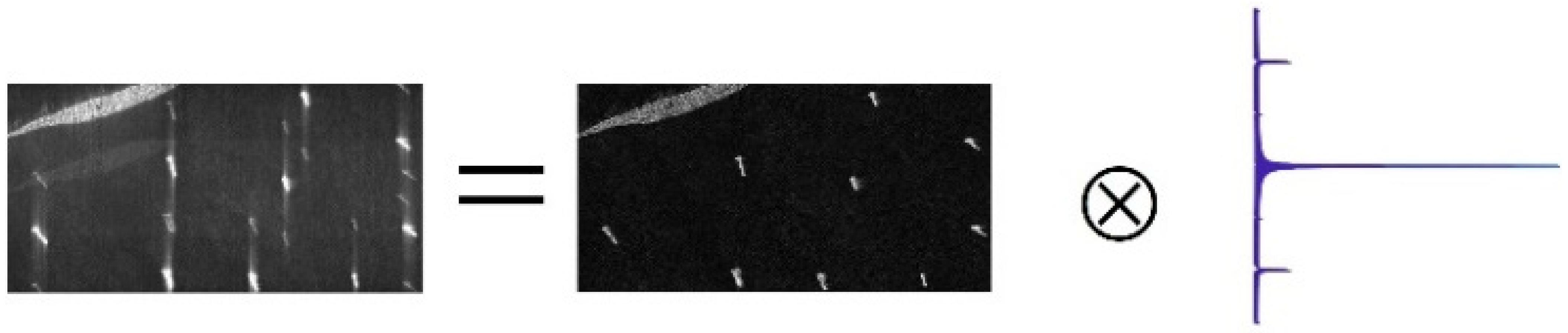
These grating lobes distort the imaging results and degrade LS-SAR image quality, increasing the difficulty of target detection and image interpretation. The position shift-invariant property of grating lobes in LS-SAR images provides a theoretical foundation and makes the convolution model an ideal mathematical model for characterizing the grating lobes-induced degradation. In this part, a general image degradation model that combines a linear convolution operation and an additive noise term is established to describe the relationship between the observed scene, the system PSF, and the degraded LS-SAR image. On this basis, the general mathematical expression shown in Equation (21) is further simplified as
I x = σ x F y q x + N x
as demonstrated in Figure 2, where I ( x ) = B P s r c τ 0 , η and B P denotes the BP imaging procedure. N x is the image noise. Figure 2 clearly illustrates the entire degradation process: the scene RCS σ x is convolved with the PSF F y q x to generate the grating lobes-degraded image I ( x ) without noise.

2.2. LS-SAR Image Grating Lobes Reduction via Deconvolution

In image processing, deconvolution, an image restoration technique, features a theoretical framework being easy to comprehend and straightforwardly derives its mathematical formulas, while providing a computationally low solution with minimal information loss. Deconvolution can simultaneously recover the observed scene and reduce grating lobes by solving the theoretically analyzed convolution model (23) in combination with the PSF of the LS-SAR system. Therefore, this paper proposes the LS-SAR image grating lobes reduction via deconvolution, where the obtaining of the PSF and the deconvolution algorithm are two important issues. The detailed procedure is shown in the following. Compared with the echo reconstructed method and the CS-based method, the proposed method solves the problem from the essential cause of grating lobes generation in LS-SAR images.

2.2.1. The Obtaining of PSF

PSF can be used as an evaluation of the system imaging performance, whose characteristics are inherently determined by the system parameters of LS-SAR, including the PRI variation strategy and azimuthal antenna pattern. The PSF mainlobe determines the azimuth impulse response width, a parameter correlated with achievable resolution. A narrower mainlobe corresponds to higher azimuthal resolution and more target details in the SAR image. In contrast, the PSF sidelobes determine the amplitude level of ambiguities in the final imaging result, where excessive sidelobes lead to severe ambiguity interference, blur target features, and degrade the overall SAR image quality. For deconvolution-based SAR image restoration and grating lobes reduction, the accuracy of the PSF is a critical and decisive factor that directly affects the effectiveness of the deconvolution. An inaccurate PSF fails to match the actual system imaging characteristics, resulting in insufficient grating lobes reduction or possibly inducing false targets in the restored image. Considering the low-oversampled staggered sampling method of LS-SAR, it is therefore necessary to obtain a physically consistent and accurate LS-SAR system PSF combined with a nonuniform PRI sampling strategy, azimuth signal processing, and azimuth antenna pattern.
The BP imaging result, which is the coherent superposition of the azimuthal response at all the sampling points, can be written as:
F y q = B P s r c τ 0 , η = t σ x p F p , q η W p , q τ 0 , η exp j 4 π λ R s e t η R p , q η + n τ 0 , η
where a certain range of time τ 0 corresponds to the range cell y = y q . PSF can be obtained. R s e t η is the slant range of the setting scene. The corresponding procedure for obtaining the PSF is as follows:
  • Select a certain range cell y q , and set the amplitude of the cell σ x p = 0 1 0 T ;
  • Calculate the slant range R s e t η n and construct the observed and reconstructed matrix
D o b = D 1 o b D p o b D P o b N × P
D r e = D 1 r e D p r e D P r e N × P
where
D p o b η n = exp j 4 π R s e t η n / λ sin c 2 L a / λ a cos R s e t η n e a r / R s e t η n θ s q
D p r e η n = exp j 4 π R s e t η n / λ
where sin c and a cos denote the sin c and anticosine function, respectively. L a is the azimuthal antenna length. R s e t η n e a r is the nearest slant range from the radar to the setting targets at a certain range cell y q . θ s q is the squint angle for the reference point at the beam center crossing time;
iii.
Construct the azimuthal signal s a z i = D o b σ x p .
iv.
Obtain the PSF F y q = D r e H s a z i .
v.
Repeat i~iv on each range cell.

2.2.2. The LS-SAR Image Grating Lobes Reduction Based on the LR Principle

Deconvolution has been adopted in image restoration applications, where the LR principle has the apparent characteristic of recovering good-quality images with no knowledge of noise power [24,25,26,27]. This characteristic is particularly valuable for SAR images, where the accurate quantification of noise power is inherently challenging. The variable practical application conditions introduce unpredictable noise and interference during signal acquisition and image processing, which makes it difficult to obtain the noise power. Therefore, this paper adopts the LR principle to address the grating lobes reduction problem.
As a nonlinear iterative algorithm for image restoration based on Bayesian probability theory, the LR deconvolution method is built on a fundamental statistical hypothesis: I x follows a Poisson distribution with σ x as the conditional parameter. Through minimizing the mean square error between the observed degraded image and the reconstructed ideal image based on the maximum likelihood estimation, the likelihood function is defined as follows:
P I ( x ) | σ ( x ) F y q = σ ( x ) F y q I ( x ) × exp σ ( x ) F y q I ( x ) !
It can be solved by minimizing Z σ ( x ) = ln P I ( x ) | σ ( x ) F y q
Z σ ( x ) = x I ( x ) ln σ ( x ) F y q + σ ( x ) F y q + ln I ( x ) !
Let Z σ ( x ) / σ ( x ) = 0 and normalize F y q , then we have
I ( x ) σ ( x ) o F y q ( x ) F y q ( x ) = 1
where o is the number of iterations, and F y q ( x ) is the transpose of F y q ( x ) . Multiplying both sides of (31) by σ ( x ) , the LR algorithm performs O iterations and converges to a stable solution, and the final result of the LR principle is as follows
σ ^ ( x ) o + 1 = σ ^ ( x ) o I ( x ) σ ^ ( x ) o F y q F y q
σ ^ ( x ) o and σ ^ ( x ) o + 1 represent the values of the restored image after the o and o + 1 iterations, respectively. The maximum likelihood estimation of the amplitude of the observed scene can be obtained by calculating (32). The observed scene on the range cell y = y q is recovered via
σ ^ x = L R I x , F y q
where L R denotes the procedure of the LR principle.

3. Results

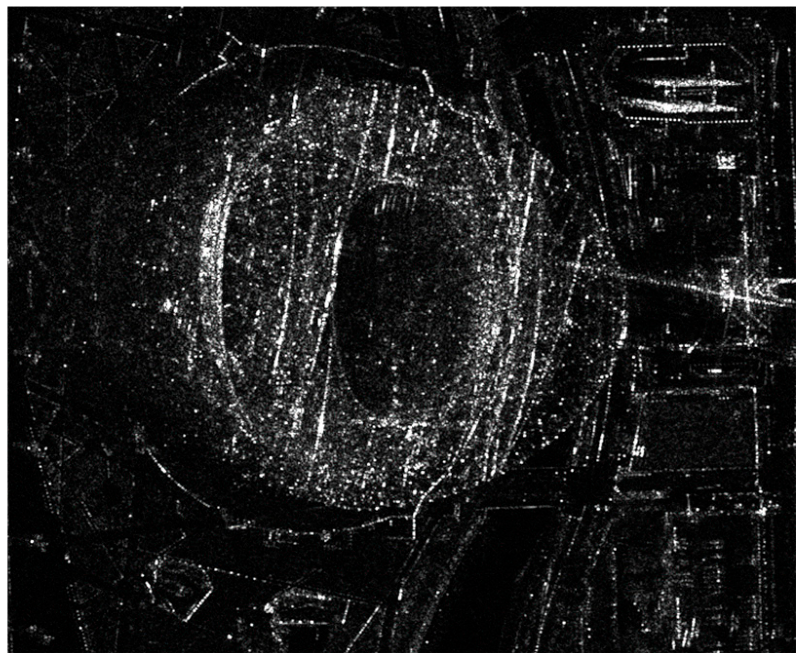
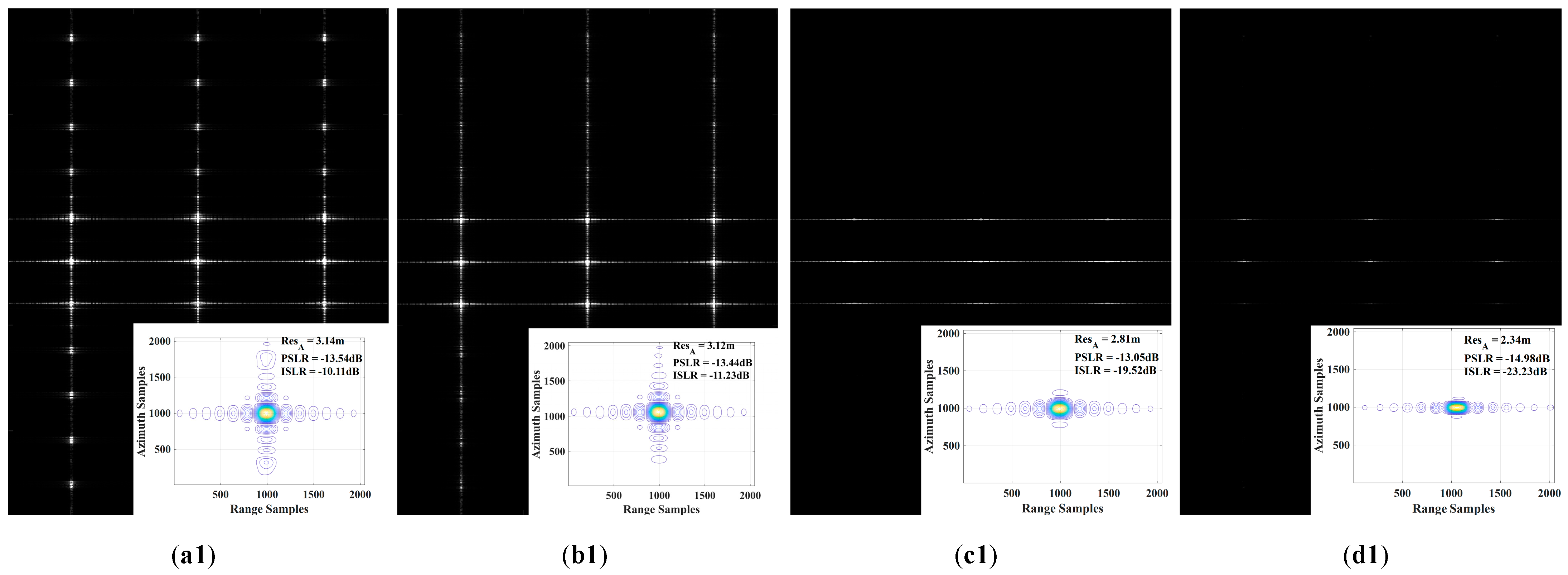
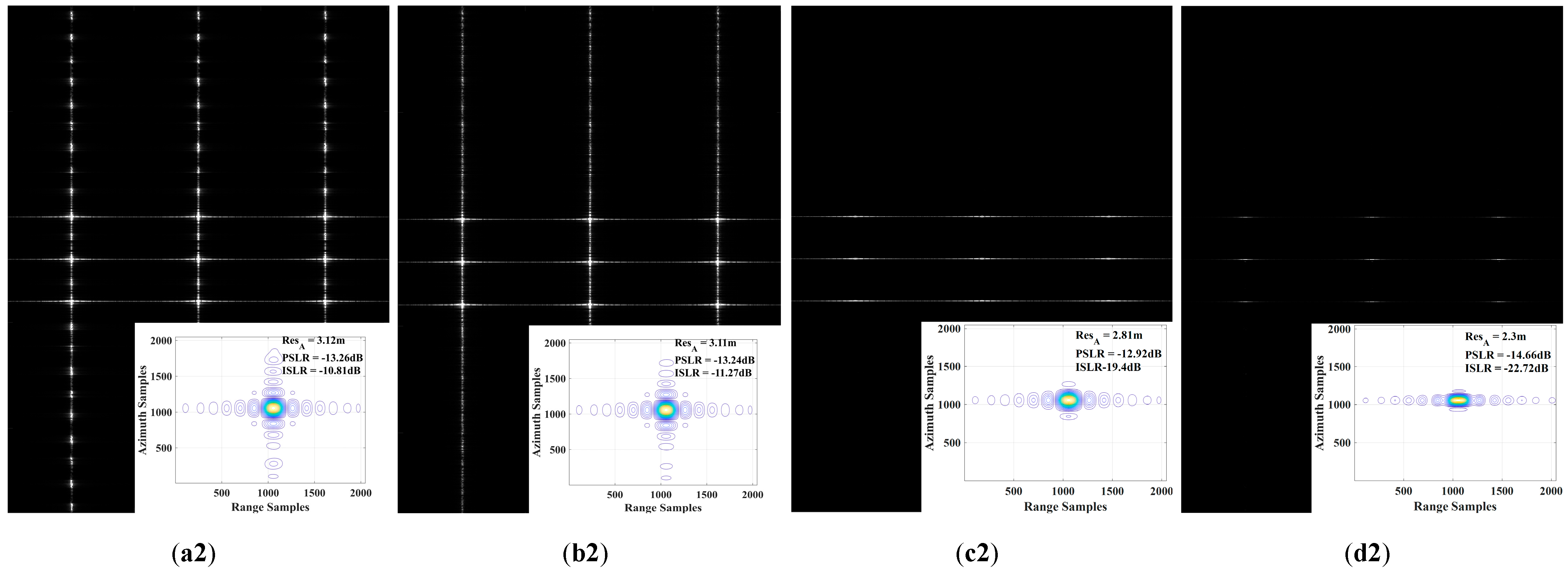
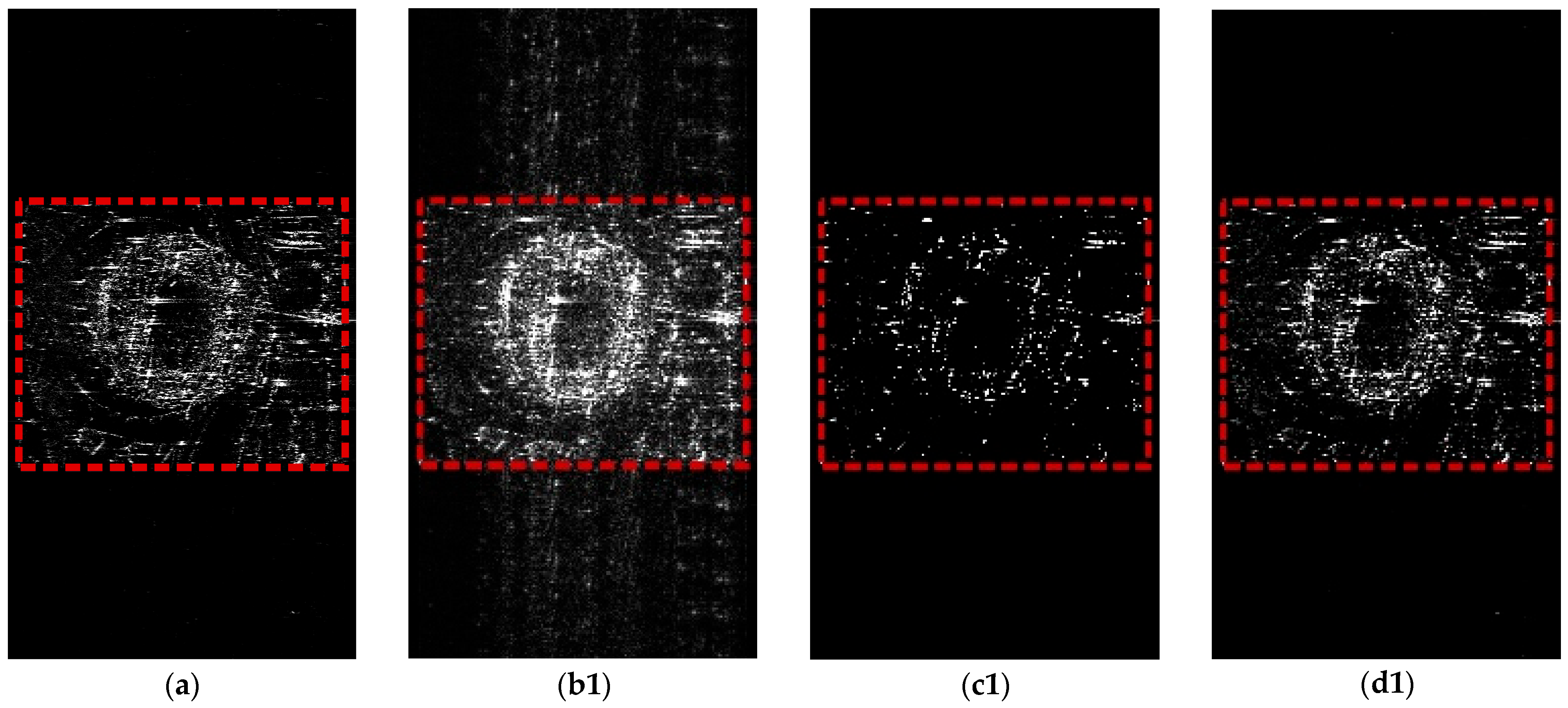
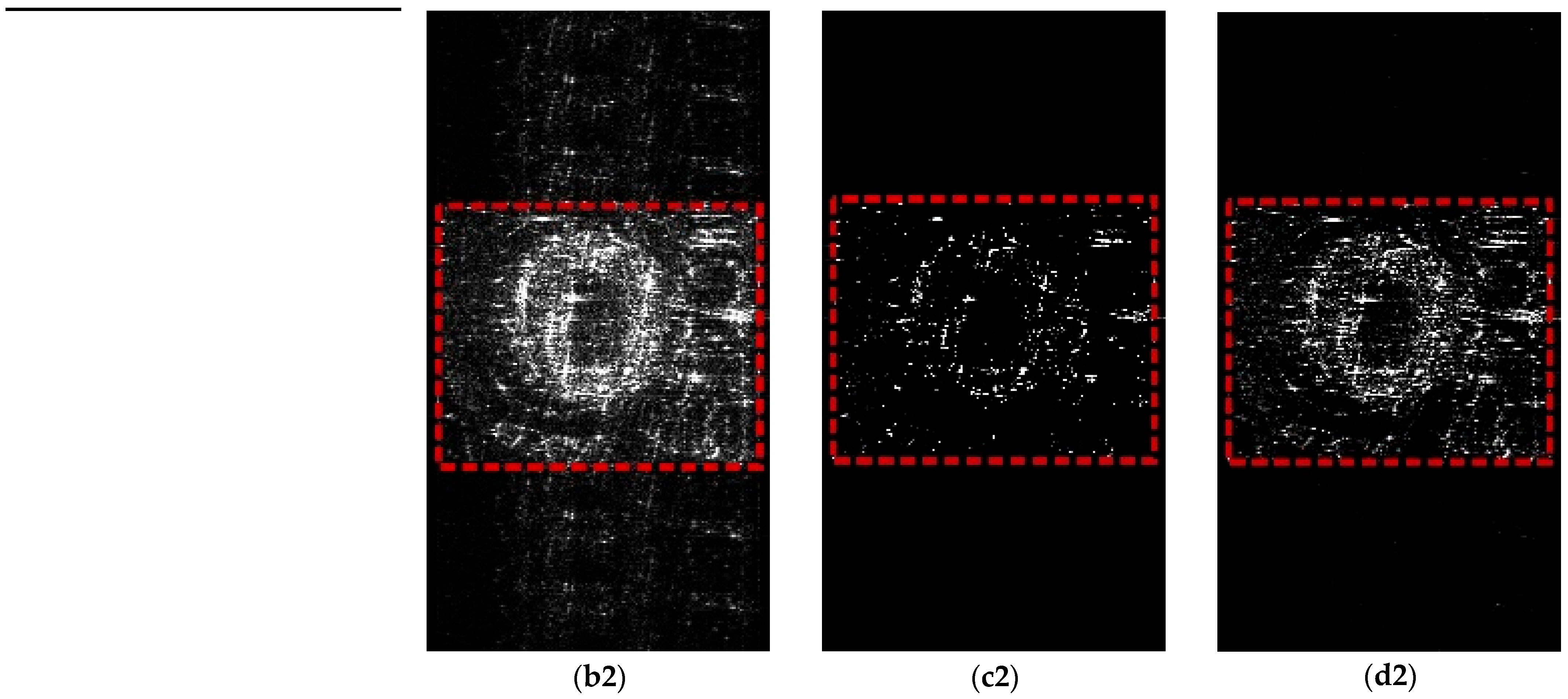
In this section, simulated experiments of point targets, real SAR images, and real measured SAR airborne data are implemented to verify the effectiveness of the proposed LS-SAR image grating lobes reduction via deconvolution. Simulated experiments use nine-point targets, and the 1m-resolution TerraSAR-X image of Beijing’s Bird Nest (acquired on 25 March 2012, shown in Figure 3) as observed scenes, with simulated parameters listed in Table 1, respectively. Additionally, real measured SAR airborne data, obtained in Guantou Ling, Guangxi Province, are used to simulate and verify in Figure 6. As shown in Figure 4 and Figure 5, two fast PRI variation sampling modes are employed in the experiments, where the first row adopts the elaborated fast variation sampling strategy, and the second row adopts the fast variation sampling strategy. For the nine-point target experiment in Figure 4, four columns are included corresponding to different imaging methods. The first column illustrates the imaging results obtained by using the best linear unbiased (BLU) estimation for azimuth resampling, followed by image focusing via the BP algorithm. The second column reconstructs the scene based on MIAA combined with BLU resampling. The third column shows the results obtained by applying the CS method to the conventional BP imaging output. The fourth column presents the reconstructed results achieved by the proposed deconvolution-based method in this paper. Regarding the column arrangement, there is a slight difference between Figure 4 and Figure 5. An additional column is added to present the original simulated scene, which serves as the reference for evaluating the imaging quality of different methods. Results of distributed scatters in Figure 5 with MIAA are not provided, as it is only effective for point targets and degrades for extended and distributed scatterers [2]. The imaging methods of the second, third, and fourth columns in Figure 5 correspond to those of the first, third, and fourth columns in Figure 4, respectively. For the point target in Figure 4, the quantitatively evaluated indexes, i.e., the resolution, the peak sidelobe ratio (PSLR) and the integrated sidelobe ratio (ISLR), of the middle point target are also given in the lower-right corner of each subplot for the central point target, facilitating the quantitative comparison of the imaging performance of different methods. For the distributed targets in Figure 5, the mean square error (MSE) and the structural similarity (SSIM) are adopted to evaluate the image quality of the region marked by the red rectangle. MSE is defined as the ratio of the error energy to the true signal energy
MSE = σ ^ σ 2 2 σ 2 2
where σ ^ is the recovered scene, i.e., the result of Equation (30). SSIM compares local patterns of pixel intensities that have been normalized for luminance and contrast [33]. In SSIM, the product of three components between the original observed scene σ and the recovered scene σ ^ is computed to estimate the image’s local quality
SSIM ( σ ^ , σ ) = α ( σ ^ , σ ) ς 1 β ( σ ^ , σ ) ς 2 γ ( σ ^ , σ ) ς 3
where α ( σ ^ , σ ) , β ( σ ^ , σ ) and γ ( σ ^ , σ ) are luminance comparison, contrast comparison, and structure comparison, respectively, and the calculation methods can be found in [33]. ς 1 , ς 2 and ς 3 are positive constants used to adjust the relative importance of these three components. A simple setting ς 1 = ς 2 = ς 3 = 1 is adopted, and this setting follows the widely used setting in the original SSIM paper [33] and the common image quality assessment. Lower values of MSE and larger values of SSIM represent better image quality.
In terms of the BLU-based method in Figure 4a and Figure 5b, ghost artifacts are visible along the azimuth in the reconstructed images, so that the azimuth grating lobes cannot be effectively suppressed. The reason for this phenomenon is that the BLU-based method performs a linear estimation and fails to fundamentally solve the problem of azimuth frequency spectrum aliasing due to the continuous PRI variation and echo data loss. So the target energy disperses in the azimuth direction, and the target contour is blurred by the grating lobes. In contrast, the CS-based method achieves image focusing and a certain degree of grating lobes suppression, and the overall imaging effect is better than that of the BLU-based method. Nevertheless, the recovery performance of the CS-based method is still inferior to that of the proposed deconvolution-based method, which is reflected in the quantitative evaluation indexes in Table 2. The limitation of the CS-based method lies in the strict dependence on the sparsity assumption of the observed scene. This method can have good performance in the reconstruction of sparse scenes such as isolated point targets, but for the distributed scene like the SAR image of the Bird Nest, the CS-based method need to filter out a large number of structural information and texture features of the scene to meet the sparsity constrain, resulting in the loss of detailed information in the reconstructed image in Figure 4b and Figure 5c. The proposed deconvolution-based method achieves the optimal imaging and recovery performance in all simulation experiments, and its effectiveness is verified by quantitative evaluation indices, as shown in Table 2. The proposed method effectively suppresses azimuth grating lobes and improves the quality of LS-SAR images while retaining the structural information and a certain degree of texture details.
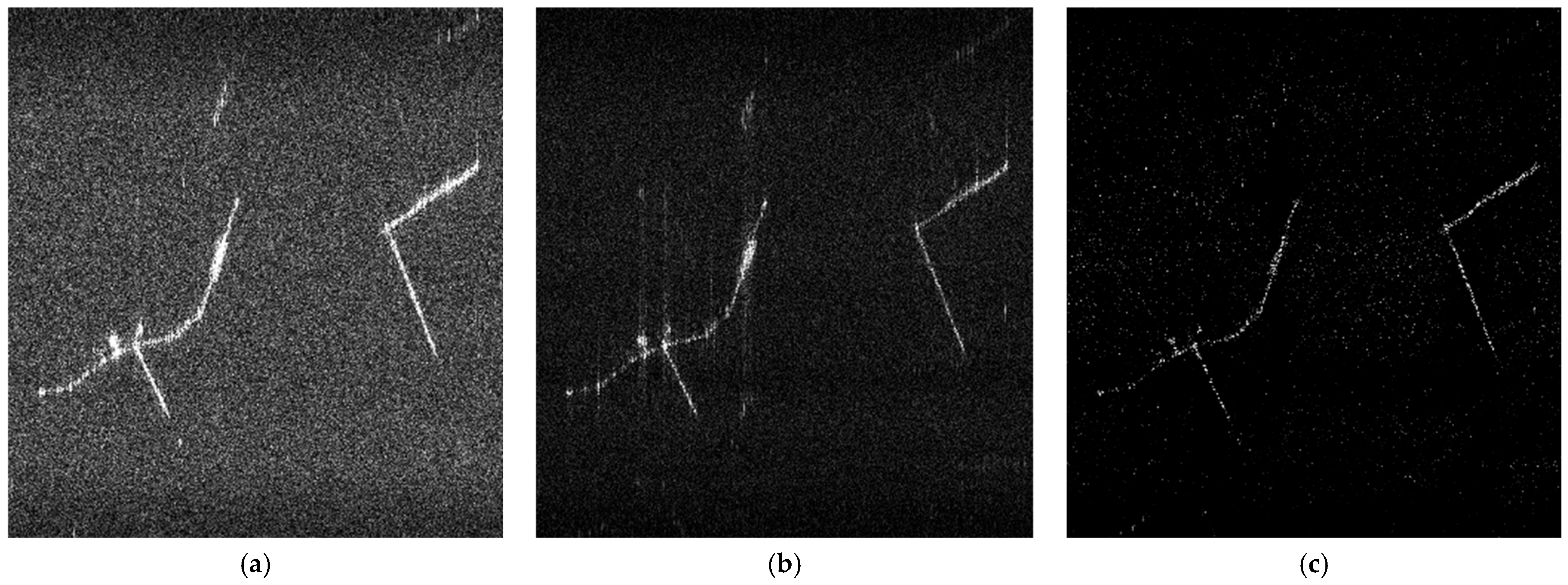
Figure 6 presents the experimental results conducted on real measured SAR airborne data, which further verifies the practical applicability and effectiveness of the proposed method in real data processing. The experimental data processing is designed with a control variable approach to demonstrate the impact of nonuniform sampling and different processing methods on LS-SAR image quality, and further, the imaging results of different processing methods are compared and analyzed. In Figure 6a, the raw data is uniformly extracted from the highly oversampled real measured SAR airborne data and satisfies the Nyquist sampling theorem to avoid the azimuth spectrum aliasing, and then it is recovered based on the BP imaging algorithm. The imaging result in Figure 6a achieves perfect focus and preserves the detailed structural information of the observed scene, which is taken as the reference. In Figure 6b,c, the raw data are nonuniformly extracted from the highly oversampled real measured SAR airborne data obeying the sampling strategy of the staggered SAR system, which simulates the actual LS-SAR observation conditions with PRI variation and echo pulse loss, making the experimental scenario consistent with the engineering application of LS-SAR. The result (b) is recovered based on the BP imaging algorithm with the BLU method on the azimuth dimension. The result (c) is recovered based on the BP imaging algorithm with the LR method on the azimuth dimension. Comparing Figure 6b,c, the imaging result of the proposed algorithm exhibits better focusing quality than that of the BLU-based method. The recovered result (b) is defocused, and the energy is spreading over azimuth. The reason for this phenomenon is that the BLU method only performs linear unbiased estimation and resampling on the nonuniform azimuth data, which cannot fundamentally reduce the azimuth grating lobes. In contrast, the grating lobes in Figure 6c are reduced, and the structural information is well preserved. The experimental results of real measured SAR airborne data verify the practical effectiveness and engineering applicability of the proposed method for LS-SAR images.

4. Discussion

This section mainly discusses the inapplicability of the proposed method to the slow PRI variation sampling strategy, the improvement of the azimuth resolution, and the iteration number of the proposed method.
(1)
The inapplicability of the proposed method to the slow PRI variation sampling strategy
The applicable scope of the proposed method should be clearly clarified. The method in this paper is applicable to fast PRI variation and elaborated fast PRI variation sampling strategies, while it is not incompatible with the slow PRI variation sampling strategy. This limitation is inherently determined by the structural characteristic of the sampling sequence, which is closely associated with the position-invariant property of grating lobes and the establishment of the convolution mathematical model.
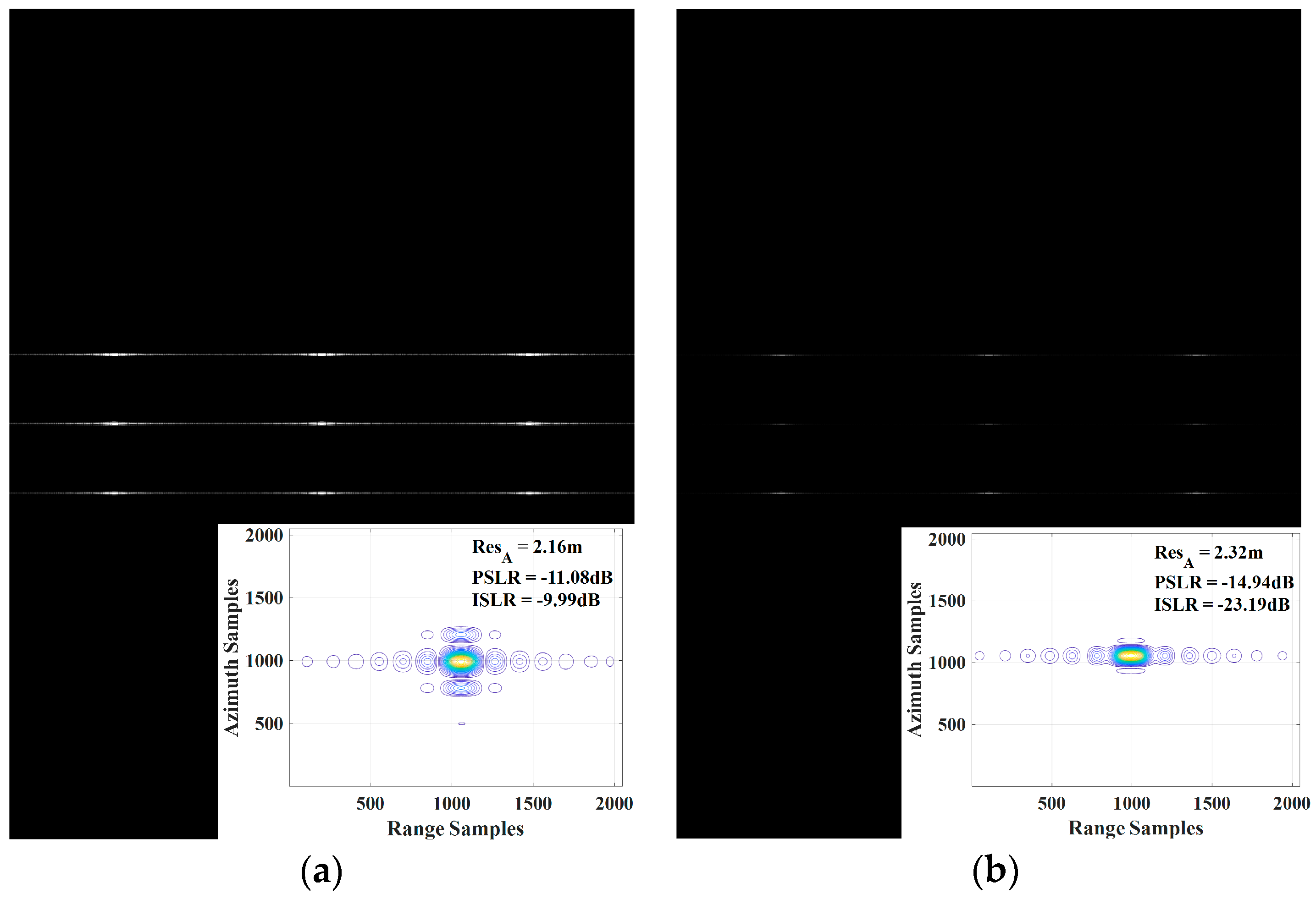
The difference between (elaborated) fast and slow PRI variation strategies lies in the periodicity of the sampling sequence. For the (elaborated) fast PRI variation sampling strategies, PRI changes rapidly within a short azimuth observation time, allowing the sampling sequence to be approximated as the sum of several periodic sequences, which is consistent with Equation (4). This periodicity enables analysis of the sampling sequence based on periodic signal theory and further validates the position-variant property of grating lobes. At the slow PRI variation sampling strategy, PRI varies over a long flight time so that there is no obvious periodicity for the sampling sequence. Correspondingly, the value of K in Equation (4) is equal to a large sampling number, and it does not satisfy the periodic sequence assumption. The absence of regularity fails to compute the frequency spectrum of the sampling strategy in Equation (13), further to derive the positions of azimuth grating lobes, and to verify their position-invariant property. Grating lobes under slow PRI variation are irregularly distributed, so the positions of grating lobes cannot be guaranteed to be consistent on different range cells, and the established convolution mathematical model is not applicable for slow PRI variation. Further, the proposed LR deconvolution-based algorithm cannot be effectively applied to the slow PRI variation sampling strategy. For the slow PRI variation strategy, the imaging performance of the proposed method is related to the position of the missing data, as illustrated in Figure 7. When data loss occurs in the middle of the receiving window, the proposed method cannot effectively suppress grating lobes, as demonstrated by PSLR and ISLR in Figure 7a. In contrast, when data is lost at the two ends of the receiving window, the imaging performance is significantly improved. This improvement can be attributed to the fact that the remaining data in this case is equivalent to a low-resolution sampled dataset and the inherent super-resolution capability of the RL algorithm. By iteratively deconvoluting the PSF, the proposed method can recover the target response with small grating lobes, leading to the superior performance observed in Figure 7b.
(2)
The improvement of the azimuth resolution
The azimuth resolution was quantitatively evaluated using the middle point target in Figure 4. The system theoretical azimuth resolution, determined by the LS-SAR system parameters in Table 1 and the uniform sampling strategy, is 3 m. As demonstrated in Table 3, the proposed LR-based method exhibits the ability to recover and enhance the actual azimuth resolution while reducing grating lobes of the LS-SAR image. The resolution improvement is of practical significance for the engineering application of high-resolution wide-swath LS-SAR systems.
For the BLU-based method in Figure 4(a1,a2), the resolution degrades due to azimuth spectrum aliasing induced by nonuniform sampling and echo pulse loss. The CS-based method in Figure 4(b1,b2) also achieves the resolution improvement by the l δ -regularized ( 0 < δ 1 ) prior, while the requirement of the sparse property constrains the reconstructed performance of the observed scene. Although point-array targets in Figure 4 are recovered based on the CS-based method, the reconstruction of the observed scene in Figure 5 loses partial structural information to satisfy the sparsity constraint. In contrast, the proposed LR-based method effectively narrows the impulse response width and improves the resolution by performing iterative deconvolution with the numerically calculated system PSF. Simultaneously, the PSLR and ISLR are also improved. The super-resolution enhancement of the proposed method mainly depends on the maximum likelihood estimation under the Poisson noise assumption, which enables reconstruction of out-of-band information [34]. Additionally, the degree of resolution improvement is closely related to the number of LR iterations. Few iterations result in the incomplete reduction in grating lobes and resolution unimprovement, and excessive iterations may generate extra noise. Therefore, the appropriate iteration number should be selected to balance resolution enhancement and noise robustness.
(3)
The iteration number of the proposed method
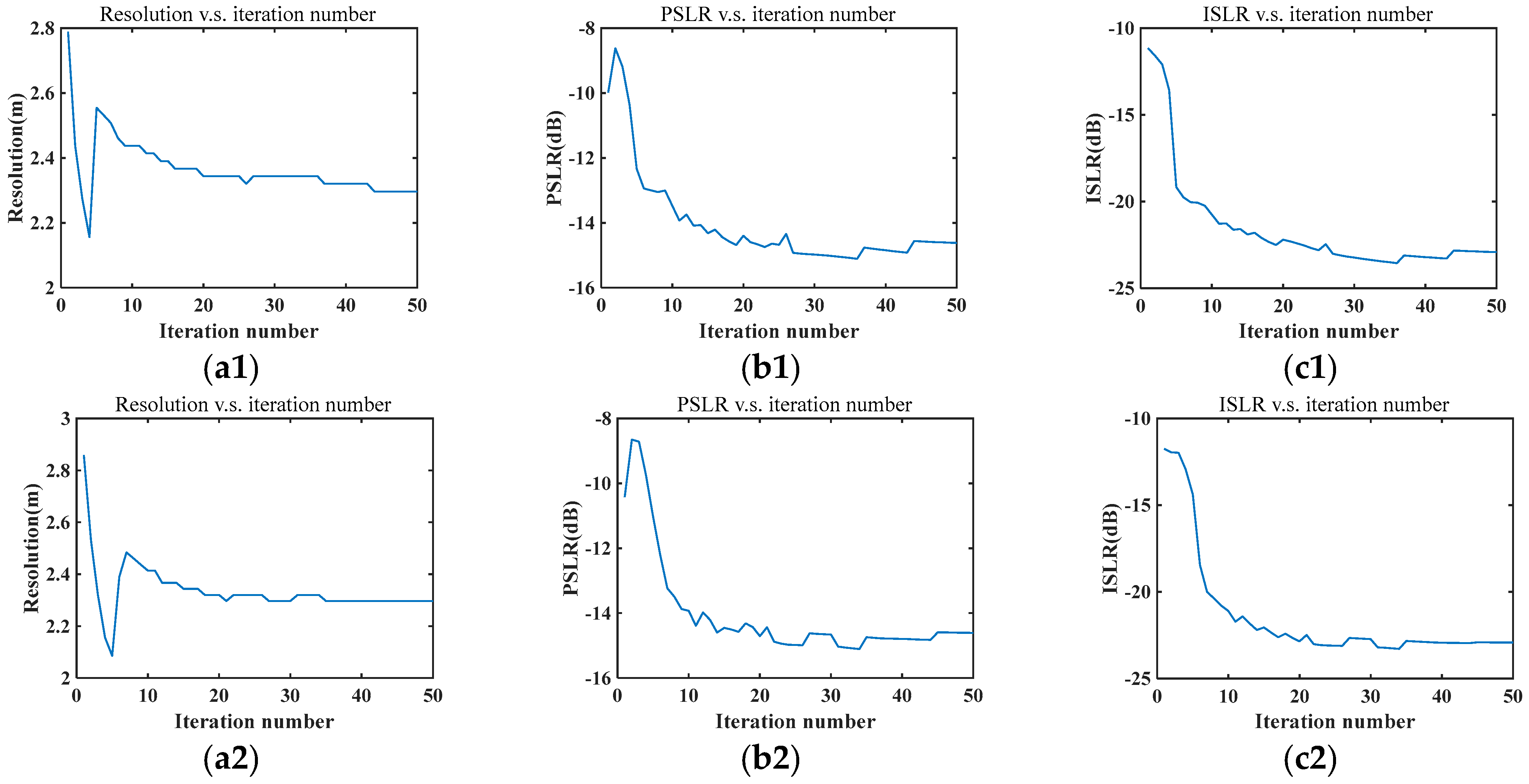
The optimal number of LR iterations depends on the recovered scene and simulation parameters (e.g., signal-to-noise ratio, target distribution, scene sparsity), and no common value is applicable to all scenarios. To analyze the parameter configuration rules, this paper selects the typical point target scene. As shown in Figure 8, the quantitatively evaluated indexes, i.e., the resolution, PSLR, and ISLR, exhibit a rapid improvement and then converge to their optimal stable values. For resolution convergence, the mainlobe width decreases rapidly in the first approximately 15 iterations, leading to a significant improvement in spatial resolution. The improvement rate slows after 20 iterations, and further, the curve converges. Similarly, PSLR and ISLR decrease rapidly in the first nearly 20 iterations, showing effective grating lobes reduction. By iteration 30, PSLR and ISLR converge to stable and near-optimal values. This makes 30 iterations a practical choice that balances imaging quality and computational efficiency, which is especially relevant for the fast and elaborate fast PRI variation sampling strategies for efficiency. This configuration ensures the algorithm achieves optimal imaging performance without unnecessary iterations or noise amplification.

5. Conclusions

In this paper, we propose a deconvolution-based method for LS-SAR image grating lobes reduction. First, azimuth grating lobes and their positions for nonuniformly sampled signals are analyzed to verify the position-invariant property, and the LS-SAR image is modeled as the convolution of the backscatter coefficient with the PSF, plus noise. Then, PSF is obtained according to the PRI variation strategy and azimuthal antenna pattern. Finally, the recovery of the observed scene and grating lobes reduction can be simultaneously achieved by deconvoluting the LS-SAR image with the acquired PSF in accordance with the LR principle. Simulated data of point-array scatters and a real SAR image demonstrate the ability to reduce azimuth grating lobes caused by a nonuniform low-oversampled azimuth sampling sequence. Results using real airborne data are also presented, which demonstrate effective reduction in grating lobes and validate the proposed method.
This paper can solve the technical problem of azimuth grating lobes and defocusing caused by the nonuniform sampling strategy of actual LS-SAR data processing, improve the imaging quality, achieve image restoration, and provide a reliable technical solution for the actual engineering application of high-resolution wide-swath LS-SAR systems.

Author Contributions

Methodology, W.C.; validation, W.C. and J.G.; formal analysis, J.G.; data curation, C.W., J.Y. and L.Y.; writing—original draft, W.C.; supervision, W.C. All authors have read and agreed to the published version of the manuscript.

Funding

This research received no external funding.

Institutional Review Board Statement

Not applicable.

Informed Consent Statement

Not applicable.

Data Availability Statement

The original contributions presented in this study are included in the article. Further inquiries can be directed to the corresponding author.

Acknowledgments

The authors would like to express their sincere gratitude to the corresponding author Jiwen Geng for his consistent support, professional guidance, and patient assistance throughout the entire research and manuscript preparation process. His expertise has been instrumental in the successful completion of this work.

Conflicts of Interest

Jiwen Geng is employed by the Nanjing Corad Electronic Equipment Company, Limited. The remaining authors declare that the research was conducted in the absence of any commercial or financial relationships that could be construed as a potential conflict of interest.

References

  1. Villano, M.; Krieger, G.; Moreira, A. Staggered SAR: High-Resolution Wide-Swath Imaging by Continuous PRI Variation. IEEE Trans. Geosci. Remote Sens. 2014, 52, 4462–4479. [Google Scholar] [CrossRef]
  2. Pinheiro, M.; Prats-Iraola, P.; Rodriguez-Cassola, M.; Villano, M. Analysis of Low-Oversampled Staggered SAR Data. IEEE J. Sel. Top. Appl. Earth Obs. Remote Sens. 2020, 13, 241–255. [Google Scholar] [CrossRef]
  3. Villano, M.; Krieger, G.; Jäger, M.; Moreira, A. Staggered SAR: Performance Analysis and Experiments with Real Data. IEEE Trans. Geosci. Remote Sens. 2017, 55, 6617–6638. [Google Scholar] [CrossRef]
  4. Hou, S.X.; Deng, Y.K.; Qiu, J.S.; Zhang, H.; Wang, W.; Lv, Z.S.; Chen, Z.; Fan, H.T.; Zhao, F.J. On Low-Oversampled ST-Staggered SAR Signal Reconstruction Scheme. IEEE Trans. Aerosp. Electron. Syst. 2025, 61, 7107–7124. [Google Scholar] [CrossRef]
  5. Chen, W.; Geng, J.; Meng, F.; Zhu, W. Low-oversampled staggered SAR imaging in present of a random PRI variation strategy. In Proceedings of the IET International Radar Conference (IRC 2023), Chongqing, China, 3–5 December 2023. [Google Scholar]
  6. Chen, W.; Zhang, L.; Geng, J.; Liu, H. Image Reconstruction for Low-Oversampled Staggered SAR Based on Bayesian Compressive Sensing. In Proceedings of the IGARSS 2023—2023 IEEE International Geoscience and Remote Sensing Symposium, Pasadena, CA, USA, 16–21 July 2023. [Google Scholar]
  7. Liu, M.Q.; Pan, J.; Zhu, J.B.; Chen, Z.C.; Zhang, B.C.; Wu, Y.R. A Sparse SAR Imaging Method for Low-Oversampled Staggered Mode via Compound Regularization. Remote Sens. 2024, 16, 1459. [Google Scholar] [CrossRef]
  8. Moreira, A.; Krieger, G.; Hajnsek, I.; Papathanassiou, K.; Younis, M.; Lopez-Dekker, P.; Huber, S.; Villano, M.; Pardini, M.; Eineder, M.; et al. Tandem-L: A Highly Innovative Bistatic SAR Mission for Global Observation of Dynamic Processes on the Earth’s Surface. IEEE Geosci. Remote Sens. Mag. 2015, 3, 8–23. [Google Scholar] [CrossRef]
  9. Rosen, P.A.; Bawden, G.W.; Barela, P.; Chapman, B.; Fattahi, H.; Jones, C.E.; Joughin, I.R.; Lavalle, M.; Lohman, R.B.; Simons, M.; et al. The NASA-ISRO SAR Mission: A summary. IEEE Geosci. Remote Sens. Mag. 2025, 13, 8–34. [Google Scholar] [CrossRef]
  10. Agrawal, K.M.; Thakur, S.; Gupta, S.; Ramanujam, V.M. NISAR S-SAR Echo Data Simulation. In Proceedings of the 2024 IEEE India Geoscience and Remote Sensing Symposium (INGARSS), Goa, India, 2–5 December 2024. [Google Scholar]
  11. Thakur, S.; Agrawal, K.M.; Ramanujam, V.M. Simulation and Analysis of Staggered PRI Sequence for NISAR. In Proceedings of the 2021 IEEE International India Geoscience and Remote Sensing Symposium (InGARSS), Ahmedabad, India, 6–10 December 2021. [Google Scholar]
  12. Pinheiro, M.; Prats, P.; Villano, M.; Rodriguez-Cassola, M.; Rosen, P.A.; Hawkins, B.; Agram, P. Processing and Performance Analysis of NASA-ISRO SAR (NISAR) Staggered Data. In Proceedings of the 2019 IEEE International Geoscience and Remote Sensing Symposium IGARSS, Yokohama, Japan, 28 July–2 August 2019. [Google Scholar]
  13. Ustalli, N.; Steinbrecher, U.; Peixoto, M.N.; Krieger, G.; Kraus, T.; Villano, M. Demonstration of Staggered Ambiguous SAR Mode for Ship Monitoring Using TerraSAR-X. In Proceedings of the 2023 8th Asia-Pacific Conference on Synthetic Aperture Radar (APSAR), Bali, Indonesia, 23–27 October 2023. [Google Scholar]
  14. Ustalli, N.; Peixoto, M.N.; Kraus, T.; Steinbrecher, U.; Krieger, G.; Villano, M. Experimental Demonstration of Staggered Ambiguous SAR Mode for Ship Monitoring With TerraSAR-X. IEEE Trans. Geosci. Remote Sens. 2023, 61, 5221816. [Google Scholar] [CrossRef]
  15. Wang, X.; Wang, R.; Deng, Y.; Wang, W.; Li, N. SAR Signal Recovery and Reconstruction in Staggered Mode with Low Oversampling Factors. IEEE Geosci. Remote Sens. Lett. 2018, 15, 704–708. [Google Scholar] [CrossRef]
  16. Huang, H.; Lin, X.; Huang, P.H.; Fan, H.T.; Liu, Y.Y.; Xi, P.L.; Liu, X.Z.; Chen, G.Z. A Novel Signal Restoration Method for Staggered-SAR System. In Proceedings of the 2022 IEEE International Geoscience and Remote Sensing Symposium (IGARSS), Kuala Lumpur, Malaysia, 17–22 July 2022. [Google Scholar]
  17. Sun, M.Z.; Wei, Q.; Yu, Y.J.; Liu, Z.; Li, W.C. Nonuniform Resampling for Staggered SAR. In Proceedings of the 2015 IEEE International Geoscience and Remote Sensing Symposium (IGARSS), Milan, Italy, 26–31 July 2015. [Google Scholar]
  18. Xu, W.; Hu, J.L.; Huang, P.P.; Tan, W.X.; Gao, Z.Q.; Dong, Y.F. Continuous PRI Variation and Phase Center Adjustment for Azimuth Uniform Sampling in Staggered SAR. IEEE Trans. Geosci. Remote Sens. 2022, 60, 52085123. [Google Scholar] [CrossRef]
  19. Wang, X.; Wang, R. A Novel Signal Processing Algorithm for Staggered SAR with Low Oversampling Factors. In Proceedings of the 11th European Conference on Synthetic Aperture Radar (EUSAR), Hamburg, Germany, 7–9 June 2016. [Google Scholar]
  20. Liu, Z.; Liao, X.; Wu, J. Image Reconstruction for Low-Oversampled Staggered SAR via HDM-FISTA. IEEE Trans. Geosci. Remote Sens. 2022, 60, 5204514. [Google Scholar] [CrossRef]
  21. Zhang, Y.; Qi, X.; Jiang, Y.; Li, H.; Liu, Z. Image Reconstruction for Low-Oversampled Staggered SAR Based on Sparsity Bayesian Learning in the Presence of a Nonlinear PRI Variation Strategy. IEEE Trans. Geosci. Remote Sens. 2022, 60, 5229824. [Google Scholar] [CrossRef]
  22. Zhou, Z.X.; Deng, Y.; Wang, W.; Jia, X.; Wang, R. Linear Bayesian Approaches for Low-Oversampled Stepwise Staggered SAR Data. IEEE Trans. Geosci. Remote Sens. 2022, 60, 5206123. [Google Scholar] [CrossRef]
  23. Liao, X.; Liu, Z.; Jin, C. Compressed Sensing Imaging for Staggered SAR with Low Oversampling Ratio. In Proceedings of the EUSAR 2021—13th European Conference on Synthetic Aperture Radar, Online, Germany, 29 March–1 April 2021. [Google Scholar]
  24. Lucy, L. An Iterative Technique for the Rectification of Observed Distribution. Astron. J. 1974, 79, 745–754. [Google Scholar] [CrossRef]
  25. Richardson, W.H. Bayesian-Based Iterative Method of Image Restoration. J. Opt. Soc. Amer. 1972, 62, 55–59. [Google Scholar] [CrossRef]
  26. He, Z.; Zhang, X.; Li, Y.; Wang, H. A Deconvolutional Reconstruction Method Based on Lucy–Richardson Algorithm for Joint Scanning Laser Thermography. IEEE Trans. Instrum. Meas. 2021, 70, 4501508. [Google Scholar] [CrossRef]
  27. Cui, Z.Y.; Ren, J.J.; Li, L.J.; Gu, J.; Zhang, J.Y. Defocusing Recovery Technology of Terahertz Image Based on 3-D PSF Simulations. IEEE Trans. Instrum. Meas. 2023, 72, 5021910. [Google Scholar] [CrossRef]
  28. Cumming, I.; Wong, F. Digital Signal Processing of Synthetic Aperture Radar Data: Algorithms and Implementation; Artech House: Norwood, MA, USA, 2004. [Google Scholar]
  29. Ozsoy, S.; Ergin, A.A. Pencil back-projection method for SAR imaging. IEEE Trans. Image Process 2009, 18, 573–581. [Google Scholar] [CrossRef] [PubMed]
  30. Durand, R.; Ginolhac, G.; Thirion-Lefevre, L.; Forster, P. Back Projection Version of Subspace Detector SAR Processors. IEEE Trans. Aerosp. Electron. Syst. 2011, 47, 1489–1497. [Google Scholar] [CrossRef]
  31. Oppenheim, A.V.; Willsky, A.S.; Nawab, S.H. Signals and Systems, 2nd ed.; Prentice-Hall: Upper Saddle River, NJ, USA, 1997. [Google Scholar]
  32. Bracewell, R.N. The Fourier Transform and Its Applications, 3rd ed.; McGraw-Hill: New York, NY, USA, 2000. [Google Scholar]
  33. Wang, Z.; Bovik, A.C.; Sheikh, H.R.; Simoncelli, E.P. Image quality assessment: From error visibility to structural similarity. IEEE Trans. Image Process. 2004, 13, 600–612. [Google Scholar] [CrossRef]
  34. Liu, Y.; Panezai, S.; Wang, Y.; Stallinga, S. Noise amplification and ill-convergence of Richardson-Lucy deconvolution. Nat. Commun. 2025, 16, 911. [Google Scholar] [CrossRef] [PubMed]
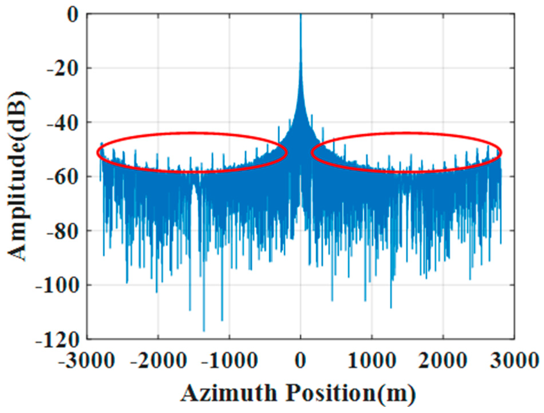
Figure 1. Nonuniformly sampled signals lead to grating lobes.
Remotesensing 18 01489 g001
Figure 2. The convolution model of the LS-SAR image grating lobes reduction.
Remotesensing 18 01489 g002
Figure 3. One SAR image is achieved by the TerraSAR-X satellite radar, and observed in Beijing’s Bird Nest.
Remotesensing 18 01489 g003
Figure 4. Experimental results of nine-point targets for the PRI variation modes, which are fast PRI variation (the first row), and elaborated fast PRI variation (the second row). (a1) The recovered image based on the BP algorithm with the BLU method for the fast PRI variation sampling strategy. (b1) The recovered image based on MIAA combined with BLU resampling for the fast PRI variation sampling strategy. (c1) The recovered image based on the BP algorithm with the CS method for the fast PRI variation sampling strategy. (d1) The recovered image based on the proposed method for the fast PRI variation sampling strategy. (a2) The recovered image based on the BP algorithm with the BLU method for the elaborated fast PRI variation sampling strategy. (b2) The recovered image based on MIAA combined with BLU resampling for the elaborated fast PRI variation sampling strategy. (c2) The recovered image based on the BP algorithm with the CS method for the elaborated fast PRI variation sampling strategy. (d2) The recovered image based on the proposed method for the elaborated fast PRI variation sampling strategy.
Remotesensing 18 01489 g004aRemotesensing 18 01489 g004b
Figure 5. The experimental results of real SAR images for the PRI variation modes, which are fast PRI variation (the first row), and elaborated fast PRI variation (the second row). (a) The simulated scene. (b1) The reconstructed image based on the BP algorithm with the BLU method for the fast PRI variation sampling strategy. (b2) The reconstructed image based on the BP algorithm with the BLU method for the elaborated fast PRI variation sampling strategy. (c1) The reconstructed image based on the BP algorithm with the CS method for the fast PRI variation sampling strategy. (c2) The reconstructed image based on the BP algorithm with the CS method for the elaborated fast PRI variation sampling strategy. (d1) The reconstructed image based on the proposed method for the fast PRI variation sampling strategy. (d2) The reconstructed image based on the proposed method for the elaborated fast PRI variation sampling strategy.
Remotesensing 18 01489 g005aRemotesensing 18 01489 g005b
Figure 6. The experiment of real measured SAR data. (a) The reconstructed image with uniformly Nyquist samples based on the BP algorithm. (b) The reconstructed image with a nonuniform LS-SAR sampling strategy based on the BP algorithm with the BLU method. (c) The reconstructed image with a nonuniform LS-SAR sampling strategy based on the BP algorithm with the LR method on the azimuth dimension.
Remotesensing 18 01489 g006
Figure 7. The recovered results of nine-point targets for the slow PRI variation based on the proposed method. For the slow PRI variation mode, the raw data may be lost in the middle and side of the receiving window corresponding to figures (a) and (b), respectively.
Remotesensing 18 01489 g007
Figure 8. Curves of quantitative performance indexes (resolution, PSLR, and ISLR) versus iteration number for the PRI variation modes, which are fast PRI variation (the first row), and elaborated fast PRI variation (the second row). (a1) resolution versus iteration number for fast PRI variation sampling strategy. (b1) PSLR versus iteration number for fast PRI variation sampling strategy. (c1) ISLR versus iteration number for fast PRI variation sampling strategy. (a2) resolution versus iteration number for elaborated fast PRI variation sampling strategy. (b2) PSLR versus iteration number for elaborated fast PRI variation sampling strategy. (c2) ISLR versus iteration number for elaborated fast PRI variation sampling strategy.
Remotesensing 18 01489 g008
Table 1. Simulated parameters and real measured SAR airborne parameters.
ParametersValue of Simulated Parameters in Figure 4 and Figure 5Value of Real Measured Airborne Parameters in Figure 6
Signal Bandwidth (MHz)44.3420
The modulated-frequency rate (MHz/us)4.43−16.8
Sampling Frequency (MHz)70500
Pulse Width (us)10
Wavelength (m)0.030.0086
Height (Km)600
Velocity (m/s)710090.30
Antenna Length (m)6
Resolution (m)3
Squint angle (°)00
The Doppler center (Hz)00
The Doppler bandwidth (Hz)2097110
The reference slant range (Km)62327.21
Mean oversampling ratio under fast PRI variation sampling strategy (Hz)1.151.45
Mean percentage of lost pulses10%21%
Table 2. Evaluated result.
MSESSIM
The observed scene for the fast PRI
variation method
(b4)1.21960.8144
(c4)1.02900.8866
The observed scene for the elaborate
PRI variation method
(b3)1.21380.8146
(c3)0.92170.8841
The lower MSE means that the pixel-level gray deviation between the reconstructed image and the original scene is minimized, and the higher SSIM indicates that the reconstructed image can accurately restore the structural characteristics of the original observed scene.
Table 3. Evaluated the indices of the middle point target in Figure 4.
CaptionResolutionPSLRISLR
BLU-based method(a1)3.14 m−13.54 dB−10.11 dB
(a2)3.12 m−13.26 dB−10.81 dB
MIAA combined with the BLU method(b1)3.12 m−13.44 dB−11.23 dB
(b2)3.11 m−13.24 dB−11.27 dB
CS-based method (c1)2.81 m−13.05 dB−19.52 dB
(c2)2.81 m−12.92 dB−19.40 dB
Proposed method(d1)2.34 m−14.98 dB−23.23 dB
(d2)2.30 m−14.66 dB−22.72 dB
Disclaimer/Publisher’s Note: The statements, opinions and data contained in all publications are solely those of the individual author(s) and contributor(s) and not of MDPI and/or the editor(s). MDPI and/or the editor(s) disclaim responsibility for any injury to people or property resulting from any ideas, methods, instructions or products referred to in the content.