A Spectral Variability and Class-Constrained Diffusion Model for Unsupervised Hyperspectral Unmixing

Highlights

What are the main findings?

• The proposed SVCDM designs a DVAE to construct a spectral library with a class constraint and prior distribution, mitigating the impact of complex SV induced by imaging characteristics.
• The conditional information is added into DM to extract endmembers across different class labels, while simultaneously optimizing abundance maps during the reverse process of the DM.

What are the implications of the main findings?

• The class labels of the endmembers on the spectral library are used as conditional information to accurately model complex SV and guide the DM in learning the distribution more accurately.
• The gradient of the log-likelihood loss is leveraged to jointly optimize abundance maps with the endmember matrix, enhancing the abundance optimization along with the updating of endmembers.

Abstract

Hyperspectral remote sensing is increasingly utilized due to its high spectral resolution and broad observational capabilities, and hyperspectral unmixing aims to decompose mixed pixels into their constituent endmembers with corresponding classes. The core research directions in this area include how to construct a proprietary spectral library and how to optimize the corresponding abundance maps. However, due to the influence of complex terrain and variable illumination conditions, hyperspectral images (HSI) exhibit significant spectral variability (SV), which undermines the performance of traditional unmixing methods. In the paper, we propose an SV and class-constrained diffusion model (SVCDM) for unsupervised hyperspectral unmixing that integrates endmember extraction and abundance optimization. Specifically, a Dirichlet-based variational autoencoder is employed to construct a spectral library from the original HSI with a class constraint and prior distribution, which subsequently guide a conditional diffusion model to learn the distribution. During the reverse process, the endmembers are iteratively updated at each time step, enhancing diversity while ensuring class consistency. Subsequently, the endmember matrix is synthesized with the original HSI to optimize the abundance maps under the linear mixing assumption. The proposed SVCDM effectively mitigates the impact of SV induced by imaging characteristics. Experimental results demonstrate that the SVCDM achieves a root mean square error (RMSE) of 0.0371 for abundance maps on a synthetic dataset and a spectral angle mapper (SAM) for endmembers of 0.0309 on the Samson dataset, outperforming existing state-of-the-art hyperspectral unmixing methods on both synthetic and real datasets.

1. Introduction

Remote sensing techniques synthesize the spectral signatures of various objects, thereby capturing the reflectance from various substances within an image, and providing a rich spectrum of information about the observed scene. Consequently, hyperspectral images (HSI) have found widespread application in fields such as mineral exploration [1], environmental monitoring [2], and urban planning [3]. Compared to multispectral imaging, HSI captures precise spectral responses across hundreds of contiguous bands, enabling the detection of subtle spectral differences between substances [4,5]. However, due to diluted photon energy, the small size of the optical aperture imposed by spatial resolution, and the inherent complexity of HSIs, a single pixel in an HSI represents a mixture of spectra from multiple endmembers [6]. This spectral mixing introduces significant challenges in several remote sensing applications, including land-cover classification [7] and object detection [8]. As a result, hyperspectral unmixing has emerged as a critical task for addressing mixed pixels, aiming to separate the constituent endmembers and estimate their corresponding proportion of a specific object in each pixel, which is defined as abundance in the context [9,10].

The linear mixing model (LMM) is a widely adopted framework in hyperspectral unmixing, which assumes that the spectrum of each pixel can be expressed as a convex combination of multiple endmembers. The corresponding coefficients are constrained by the abundance non-negativity constraint (ANC) and the sum-to-one constraint (ASC) [11,12]. A variety of methods have been developed based on the LMM, including geometry-based approaches under the pure-pixel assumption, such as pixel purity index (PPI) [13], N-FINDR [14] and vertex component analysis (VCA) [15], as well as minimum volume-based approaches like minimum volume simplex analysis (MVSA) [16] and minimum volume enclosing simplex (MVES) [17]. These approaches improve the physical interpretability of hyperspectral unmixing by constructing minimal simplices that enclose the pure pixels. However, the LMM fails to account for nonlinear mixing effects and endmember variability (EV) under varying spatial resolutions and imaging conditions [18,19], including spectral variability (SV) induced by factors such as illumination conditions, sensor viewing angles, or imaging characteristics of the objects [20,21]. As a result, hyperspectral unmixing under the LMM becomes a nonconvex optimization problem, thereby limiting its effectiveness in real-world applications [22,23].

To overcome the limitations of the LMM in effectively modeling EV, several extended versions of the LMM have been proposed. These models typically introduce variable parameters into the endmember representations to capture EV. For instance, a perturbation term is utilized to account for intensity variations caused by nonlinear mixing effects, while additive perturbations or linear transformation matrices are incorporated to flexibly model the shape distortions of endmembers [24]. Compared to the traditional LMM, these extended models demonstrate superior adaptability and robustness, resulting in improved unmixing performance under non-ideal lighting conditions [25]. However, these methods rely on parametric spectral modeling, such as linear scaling or band-wise projection, which restrict their capacity to fully capture the diversity and nonlinearity of endmembers [26].

Generative frameworks have shown significant potential in capturing the underlying structure of high-dimensional data by modeling complex distributions. These frameworks are capable of generating new samples by learning latent representations from limited training data, thereby enabling effective data reconstruction and augmentation [27]. To enhance the modeling of EV, researchers have increasingly focused on generative approaches for hyperspectral unmixing, including variational autoencoders (VAEs) and generative adversarial networks (GANs) [28,29,30]. Notably, an endmember-oriented Transformer network (EOT-Net) [31] and a probabilistic generative model for spectral unmixing (PGMSU) [32] employ an encoder–decoder architecture, where the encoder learns the latent representations of endmembers, simultaneously optimizing the abundance maps. However, due to the lack of prior knowledge and instability during training, these methods produce endmembers that are inconsistent with the corresponding classes, limiting the effectiveness of hyperspectral unmixing.

In contrast to earlier generative frameworks, the diffusion model (DM) exhibits superior stability and generative capacity, particularly in the presence of noisy data [33,34]. Consequently, DMs have found applications in image generation and signal reconstruction, and recent research has extended their use to hyperspectral unmixing with the aim of more effectively characterizing endmembers [35,36]. In these approaches, prior knowledge derived from the existing spectral library is integrated with likelihood estimation based on the LMM during the reverse process. This integration facilitates the handling of endmembers and abundances from the prior distribution, overcoming the limitations of sparse regression by enabling the generation of new endmembers within a continuous distribution. As a result, DMs are better equipped to address SV induced by factors such as illumination conditions and sensor viewing angles [37,38]. However, current diffusion-based methods for hyperspectral unmixing lack sufficient conditional information to guide the generation period, making it difficult to accurately distinguish similar classes of endmembers.

In this paper, we propose an SV and class-constrained DM (SVCDM) for unsupervised hyperspectral unmixing that integrates endmember extraction and abundance optimization. The model consists of two parts: a Dirichlet-based VAE (DVAE) is designed to construct a spectral library with a class constraint and prior distribution. Furthermore, a DM with conditional information is employed, combining class labels as conditional information to learn the distribution and progressively extract endmembers through the reverse process. Simultaneously, at each time step, the endmember matrix is synthesized with the original HSI to optimize the abundance maps, enabling joint and continuous optimization of abundances. The main contributions of this paper are listed as follows:

• A DVAE is designed to construct a spectral library with a class constraint and prior distribution, mitigating the impact of SV induced by imaging characteristics.
• A DM with conditional information is employed to extract endmembers across different class labels, while simultaneously optimizing abundance maps during the reverse process of the DM.

The remainder of this paper is organized as follows. Section 2 reviews the related work and background of hyperspectral unmixing and provides the motivation. Section 3 describes the proposed methodology and its implementation details. Section 4 presents the experimental results, followed by a discussion of ablation studies. Finally, Section 5 concludes the paper and highlights potential avenues for future research.

2. Related Work and Background

In this section, we review various hyperspectral unmixing methods, categorizing them into four types: LMM-based, extended versions of LMM-based, generative framework-based, and DM-based methods. Additionally, we discuss the motivation behind the proposed method.

2.1. Hperspectral Unmixing with LMM

The LMM is one of the fundamental models in hyperspectral unmixing. It assumes that the spectrum of each pixel is represented as a linear combination of several endmembers, with an additive noise component [39]. The mathematical formulation is given as follows: where $\mathbf{X}\in {\mathbb{R}}^{L\times 1}$ denotes an observed pixel with L bands, $\mathbf{W}\in {\mathbb{R}}^{L\times P}$ is the P endmembers, with each column indicating the proportion of each endmember, $\mathbf{H}\in {\mathbb{R}}^{P\times 1}$ is the abundance coefficients, and $\mathbf{E}\in {\mathbb{R}}^{L\times 1}$ represents the additive noise.

$$\mathbf{X}=\mathbf{W}·\mathbf{H}+\mathbf{E}$$

(1)

To ensure the physical interpretability of hyperspectral unmixing, the LMM typically incorporates the following constraints: the Endmember Non-Negativity Constraint (ENC), ANC and ASC, as formulated below:

$$\left\{\begin{array}{c}{\mathbf{W}}_i\ge 0,\hfill \\ {\mathbf{H}}_i\ge 0,\hfill \\ {\displaystyle {\displaystyle \sum _{i=1}^P}{\mathbf{H}}_i=1}\hfill \end{array}\right.$$

(2)

where $1\le i\le P$ denotes the i-th endmember. Due to its straightforward implementation and physical interpretability, the LMM has been widely used in hyperspectral unmixing. However, the core assumption—that all pixels share a fixed set of endmembers—fails to account for SV [40]. Consequently, the LMM faces difficulties in accurately extracting endmembers when significant SV exists across HSIs.

2.2. Extended Versions of the LMM for Hyperspectral Unmixing

To improve the standard LMM in capturing SV, several extended versions of the LMM have been proposed. For example, Brezini et al. [41] proposed a structured additively tuned LMM with an associated unmixing framkwork, and a cost function was optimized with iterative and multiplicative update rules by additional constraints that controlled the SV. Thouvenin et al. [42] introduced an LMM that explicitly accounted for spatial and spectral EVs with an additive spatially varying perturbation matrix, alternating marginal minimizations of an appropriately regularized cost function. In recent years, Hong et al. [43] introduced an augmented LMM (ALMM), which incorporated an SV dictionary to model the mismatch between the original and estimated spectra with penalty parameters, introducing a sparsity penalty within the optimization process, and enabling effective separation of the variability components associated with the endmembers. Drumetz et al. [44] proposed an extended LMM (ELMM) that modeled SV induced by illumination conditions by assigning a scaling factor to each endmember with the Hapke model, relaxing the rigid simplex assumption by allowing endmembers to be independently scaled across different pixels, thereby providing greater flexibility in modeling SV. Imbiriba et al. [45] proposed a generalized LMM (GLMM), which modeled SV across different bands by introducing pixel-specific linear transformation matrices. This method allowed for more flexible modeling of SV across bands. However, the aforementioned methods primarily rely on parametric spectral modeling that remain fixed during endmember updates, making it challenging to effectively model complex SV.

2.3. Generative Hyperspectral Unmixing

Generative framework introduces pixel-wise latent representation to model SV [46]. Specifically, let ${\mathbf{y}}_n$ denote the vector of the n-th pixel in the HSI. The framework assumes that ${\mathbf{y}}_n$ follows a multivariate Gaussian distribution:

$${\mathbf{y}}_n\sim \mathcal{N}({\mathbf{M}}_n{\mathbf{a}}_n,\mathsf{\Lambda })$$

(3)

where ${\mathbf{M}}_n$ represents the endmember matrix associated with pixel n, ${\mathbf{a}}_n$ is the corresponding abundance vector satisfying the ASC and ANC, and $\mathbf{\Lambda }={\lambda }_0\mathbf{I}$ denotes the noise covariance matrix.

A latent vector ${\mathbf{z}}_n$ is introduced for each pixel to represent implicit factors influencing the pixel’s spectrum. A nonlinear generative function $f_{\theta }(·)$ is then used to produce the vectorized form of the pixel-specific endmember matrix:

$$\mathrm{vec}\left({\mathbf{M}}_n\right)=f_{\theta }\left({\mathbf{z}}_n\right)$$

(4)

where $\mathrm{vec}\left({\mathbf{M}}_n\right)$ denotes the vectorization of ${\mathbf{M}}_n$ by stacking its columns. This process enables the framework to better model SV. However, such methods lack explicit prior knowledge, which compromises the physical interpretability of hyperspectral unmixing.

2.4. DM-Based Hyperspectral Unmixing

The core principle of the DM lies in constructing a pair of forward and reverse stochastic processes, where the forward process progressively adds noise, and the reverse process learns to denoise, ultimately recovering clean samples from the learned distribution. Chen et al. [47] proposed a diffusion-based HSI classification framework, SpectralDiff, which designed a DM over spatially partitioned image blocks to capture discriminative spectral–spatial characteristics, leveraging the generalization ability of DMs to progressively generate latent representations. Yu et al. [48] integrated the DM into HSI classification, with UnmixDiff, which trained the model on abundance maps derived from hyperspectral unmixing and subsequently synthesized HSIs aligning with the learned abundance maps during the reverse process. Additionally, Deng et al. [49] introduced a DM-based hyperspectral unmixing method, DiffUn, which incorporated DM into hyperspectral unmixing by learning the prior distribution of endmembers from a reference spectral library, performing joint sampling of endmembers and abundances during the reverse process. However, DM-based hyperspectral unmixing methods generally lack conditional information derived from class labels of endmembers, which limits the flexibility of the unmixing process and reduces discriminability when handling similar endmembers with different classes.

2.5. Motivation

In summary, extended versions of the LMM utilize scaling or perturbation factors to model SV to some extent. However, these models still depend on predefined parametric forms, which limit their ability to effectively capture nonlinear or complex SV. Moreover, generative frameworks introduce pixel-wise latent representations to model SV, but the forward process in these frameworks lacks explicit prior knowledge, which compromises their physical interpretability and results in weak class consistency with endmembers. DM-based hyperspectral unmixing, which jointly handle endmembers and abundances during the reverse process, offer advantages in modeling SV. However, they face challenges in distinguishing the spectral characteristics of endmembers from different classes, limiting their discriminability between endmembers.

The proposed SVCDM constructs a spectral library with a class constraint and prior distribution using a DVAE and incorporates class labels as conditional information. This combination allows the DM to accurately capture the spectral characteristics of endmembers, enhancing the distinguishability between endmembers from different classes. Additionally, at each time step of the reverse process, the reconstruction error between the output and representative spectra is introduced as a likelihood term to guide the reverse process, thereby enabling joint abundance optimization alongside the updating of endmembers.

3. Methodologies

The architecture of the proposed SVCDM is illustrated in Figure 1 and consists of two primary parts: (1) a DVAE for spectral library construction, and (2) a DM with conditional information for endmember extraction with dynamic abundance optimization. In details, a DVAE is designed to construct a spectral library with a class constraint and prior distribution, where the representative spectra extracted from the original HSI serve as training samples and their associated classes are used as conditional information to guide the DM in learning the prior distribution of endmembers corresponding to different classes. During the reverse process, the gradient of the log-likelihood with respect to the endmembers is computed based on the linear mixing assumption and integrated with the prior distribution, jointly guiding the reverse process. By integrating the endmember matrix with the original HSI, the abundance maps are dynamically optimized in parallel with the updating of endmembers.

3.1. Spectral Library Construction

In the construction of the spectral library, local VCA is applied to HSI blocks, which limits global class consistency and fails to capture SV. The core idea of the proposed DVAE is to encode the class constraint and prior distribution as the knowledge via Dirichlet distribution, enforcing the ENC and constructing a spectral library within realistic spectral bounds.

The VAE consists of two components: the encoder and the decoder. The encoder learns the latent representation of spectra while simultaneously estimating the components of different classes within each mixed pixel of the HSI. The decoder then maps the latent representation to the knowledge and associates them with the corresponding components to synthesize the pixel through the LMM.

Given an input mixed pixel $\mathbf{x}\in {\mathbb{R}}^L$, the encoder outputs $\mathit{\alpha }\in {\mathbb{R}}^C$ as the parameters of Dirichlet distribution for the representative spectra. To address the non-differentiability of the Dirichlet distribution during sampling, reparameterization is applied using the Gamma distribution, from which the latent representation of spectra is sampled. The sampling process is expressed as follows:

$$z_c={\displaystyle \frac{g_c}{{\sum }_{j=1}^c{g}_j}}$$

(5)

where $g_c,g_j$ denote the random variables sampled from $\mathrm{Gamma}({\alpha }_c,1)$, which are used to construct the latent representation for Dirichlet distribution. Here, j is the index variable, c is the number of classes, and ${\alpha }_c$ is used to control the concentration of the components in latent representation. The Dirichlet distribution enforces the ENC limit $\mathbf{z}$ into $(0,1)$, thereby enhancing the physical meaning of the latent representation $\mathbf{z}$.

Furthermore, after assessing the latent representation $\mathbf{z}$, the reconstruction term in the variation is interpreted as the expectation of the conditional likelihood under the prior distribution ${\mathbb{E}}_{q_{\varphi }\left(\mathbf{z}\right|\mathbf{x})}\left[log{p}_{\theta }\left(\mathbf{x}\right|\mathbf{z})\right]$.

This term measures that the representative spectra generated from the latent representation $\mathbf{z}$ reconstruct the mixed pixel $\mathbf{x}$. A higher value indicates that the spectra are more consistent with the observed spectral characteristics. Since the above expectation is generally intractable, a Monte Carlo approximation is adopted to estimate the expectation. Specifically, a single sample is drawn from the prior distribution, which is approximated as

$${\mathbb{E}}_{q_{\varphi }\left(\mathbf{z}\right|\mathbf{x})}\left[log{p}_{\theta }\left(\mathbf{x}\right|\mathbf{z})\right]\approx log{p}_{\theta }\left(\mathbf{x}\right|\mathbf{z})$$

(6)

Through this sampling process, the matrix ${\mathbf{M}}_c$ is computed by the latent representation ${\mathbf{z}}_c$ and is then partitioned into c groups, which are used to construct the spectral library, providing prior distribution of the representative spectral composition, and stronger support for the DM in modeling EV.

3.2. Diffusional Endmember Extraction

After constructing the spectral library, the network is reformulated as a diffusion-based endmember extraction framework. Specifically, the DM is trained conditionally across different classes, with the spectrum of specific classes serving as inputs to represent the class-wise endmembers. This enables the extraction of diverse and class-consistent endmembers from noise. The forward process of the DM is inspired by nonequilibrium thermodynamics and is modeled as a Markov chain, which progressively adds Gaussian noise to representative spectra, thereby transforming them into a Gaussian distribution. The Gaussian noise is incrementally introduced over T time steps, resulting in noisy spectra ${\mathbf{x}}_1,\dots ,{\mathbf{x}}_t$. Let $\mathbf{x}$ denote the representative spectrum for a specific class at time step $t=0$. At time step t of the forward process, Gaussian noise controlled by variance schedule ${\beta }_t$ is added to the representative spectrum, and the distribution of noisy spectrum is expressed as

$$q({\mathbf{x}}_t\mid {\mathbf{x}}_{t-1})=\mathcal{N}({\mathbf{x}}_t;\sqrt{{\alpha }_t}{\mathbf{x}}_{t-1},(1-{\alpha }_t)\mathbf{I})$$

(7)

where ${\mathbf{x}}_{t-1}$ and ${\mathbf{x}}_t$ denote the noisy spectrum at time steps $t-1$ and t, respectively, ${\alpha }_t$ is calculated by $1-{\beta }_t$, and $\mathbf{I}$ is the unit covariance matrix.

The amplitude of Gaussian noise added at time step t is controlled by the variance scheduling parameter ${\alpha }_t$. At time step 1, the forward process is defined as

$${\mathbf{x}}_1=\sqrt{{\alpha }_1}{\mathbf{x}}_0+\sqrt{1-{\alpha }_1}\mathit{ϵ},\mathit{ϵ}\sim \mathcal{N}(\mathbf{0},\mathbf{I})$$

(8)

where ${\mathbf{x}}_0$ and ${\mathbf{x}}_1$ denote the noisy spectrum at time step 0 and 1, respectively, ${\alpha }_t$ is computed by $1-{\beta }_t$, and $\mathit{ϵ}$ is the added Gaussian noise. From Equations (7) and (8), it is deduced that ${\mathbf{x}}_t$ is computed directly from the representative spectrum ${\mathbf{x}}_0$ with noise $\mathit{ϵ}$:

$$\left\{\begin{array}{cc}\hfill {\mathbf{x}}_t& ={\overline{\alpha }}_t{\mathbf{x}}_0+\sqrt{1-{\overline{\alpha }}_t}\mathit{ϵ},\hfill \\ \hfill {\overline{\alpha }}_t& ={\displaystyle \prod _{i=1}^t}{\alpha }_i\hfill \end{array}\right.$$

(9)

where ${\overline{\alpha }}_t$ denotes the accumulation of $\alpha$ from time step 1 to t. Thus, the noisy spectrum ${\mathbf{x}}_t$ is represented by a linear combination of ${\mathbf{x}}_0$ and $\mathit{ϵ}$. The prior distribution of the forward process is utilized to recover the endmember from the noise by ${\nabla }_{{\mathbf{x}}_t}logp\left({\mathbf{x}}_t\right)$.

The reverse process of the DM is regarded as the inversion of the Markov chain. In the reverse process, the DM progressively denoises the endmembers corrupted by Gaussian noise, ultimately extracting endmembers corresponding to specific classes. The goal is to analyze and recover the underlying distribution. Given the noisy spectrum ${\mathbf{x}}_t$ and the condition c at the current time step t, the distribution at the previous time step is predicted. Assuming that it obeys a Gaussian distribution, the expression is listed as follows:

$$p_{\theta }({\mathbf{x}}_{t-1}\mid {\mathbf{x}}_t,c)=\mathcal{N}\left({\mathbf{x}}_{t-1};{\mathsf{\mu }}_{\theta }({\mathbf{x}}_t,c,t),{\sigma }_t^2\mathbf{I}\right)$$

(10)

where ${\mathsf{\mu }}_{\theta }({\mathbf{x}}_t,c,t)$ and ${\sigma }_t^2$ are the mean and variance of distribution $p_{\theta }({\mathbf{x}}_{t-1}\mid {\mathbf{x}}_t,c)$. Meanwhile, a module is trained to predict the added Gaussian noise $\mathit{ϵ}$. The expression for the mean of the distribution is as follows:

$${\mathsf{\mu }}_{\theta }({\mathbf{x}}_t,c,t)={\displaystyle \frac{1}{\sqrt{{\alpha }_t}}}\left({\mathbf{x}}_t-{\displaystyle \frac{1-{\alpha }_t}{\sqrt{1-{\overline{\alpha }}_t}}}{\widehat{\mathit{ϵ}}}_{\theta }({\mathbf{x}}_t,c,t)\right)$$

(11)

where ${\widehat{\mathit{ϵ}}}_{\theta }({\mathbf{x}}_t,c,t)$ denotes the predicted noise; ${\alpha }_t$ is the noise scheduling coefficient, which is calculated by $1-{\beta }_t$; and ${\overline{\alpha }}_t$ denotes the accumulation of noise scheduling coefficients from time step 1 to T.

Meanwhile, the noise variance ${\sigma }_t^2$ in the reverse process is determined by the noise scheduling factor ${\alpha }_t$ with the following expression:

$${\sigma }_t^2={\displaystyle \frac{1-{\overline{\alpha }}_{t-1}}{1-{\overline{\alpha }}_t}}(1-{\alpha }_t)$$

(12)

According to the forward process, the prediction of the original endmember matrix from step t is given by

$${\mathbf{S}}_{0/t}={\displaystyle \frac{1}{{\overline{\alpha }}_t}}\left({\mathbf{S}}_{0/t}-\sqrt{1-{\overline{\alpha }}_t}\mathit{ϵ}\right)$$

(13)

where ${\mathbf{S}}_t$ is the endmember matrix at time step t, and ${\mathbf{S}}_{0/t}$ denotes the predicted endmember matrix.

To guide the direction of updating of endmembers at each time step of the reverse process, the gradient of log-likelihood is calculated [50,51,52]. The gradient term is defined by the following equation:

$${\nabla }_{{\mathbf{S}}_{0/t}}logp({\mathbf{S}}_{0/t}\mid \mathbf{Y},{\mathbf{H}}_t)={(\mathbf{Y}-{\mathbf{H}}_t{\mathbf{S}}_{0/t}^{\top })}^{\top }{\mathbf{H}}_t$$

(14)

The gradient ${\nabla }_{{\mathbf{S}}_{0/t}}logp({\mathbf{S}}_{0/t}\mid \mathbf{Y},{\mathbf{H}}_t)$ is computed by minimizing the approximation error between $\mathbf{Y}$ and the linear combination of the endmember matrix ${\mathbf{S}}_{0/t}$ with the corresponding abundance map ${\mathbf{H}}_t$, thereby guiding the posterior denoising of endmembers to strike a balance between endmember diversity and reconstruction error.

Building upon this, to ensure that the output closely aligns with the representative spectra, the mean square error (MSE) between the output and representative spectra is employed to enhance class consistency. The gradient term is expressed as follows:

$${\nabla }_{{\mathbf{S}}_{0/t}}^{\mathrm{MSE}}={\displaystyle \frac{2}{L}}({\mathbf{S}}_{0/t}-\widehat{\mathbf{S}})$$

(15)

where $\widehat{\mathbf{S}}$ denotes the endmember matrix constructed from class-wise mean representative spectra and L is the number of bands.

After adding the weighting coefficients ${\lambda }_{mse}$, the integrated gradient bootstrap is updated as

$${\nabla }_{{\mathbf{S}}_{0/t}}^{\mathrm{total}}={\nabla }_{{\mathbf{S}}_{0/t}}logp({\mathbf{S}}_{0/t}\mid \mathbf{Y},{\mathbf{H}}_t)+{\lambda }_{mse}{\nabla }_{{\mathbf{S}}_{0/t}}^{\mathrm{MSE}}$$

(16)

Combined with the gradient term, the posterior denoising of endmembers during the reverse process of the DM is defined as

$${\mathbf{x}}_{t-1}={\mathsf{\mu }}_{\theta }({\mathbf{x}}_t,c,t)+{\nabla }_{{\mathbf{S}}_{0/t}}^{\mathrm{total}}+{\sigma }_t\mathbf{z}$$

(17)

where $\mathbf{z}$ is the standard Gaussian noise.

3.3. Dynamic Abundance Optimization

Based on the iterative updating of the endmember matrix during the reverse process, the corresponding abundance map is optimized at each time interval $\mathsf{\Delta }t$ using the current endmember matrix and the original HSI. Specifically, the minimization objective is formulated as

$$min\parallel \mathbf{Y}-{\mathbf{S}}_{0/t}{\mathbf{H}}_t^{\top }{\parallel }_F^2+{\lambda }_{spare}R\left({\mathbf{H}}_t\right)$$

(18)

where $\mathbf{Y}$ is the original HSI, $\mathbf{H}$ is the abundance map, and ${\mathbf{S}}_{0/t}$ is the endmember matrix at time step t. ${\lambda }_{\mathrm{sparse}}$ is the sparsity penalty weight. $R\left({\mathbf{H}}_t\right)$ is a regularization term that promotes sparsity in the abundance map. It is formulated as

$$\left\{\begin{array}{c}R\left({\mathbf{H}}_t\right)={\parallel {\mathbf{H}}_t\parallel }_1,\hfill \\ {\mathbf{H}}_t>0,{\mathbf{H}}_t^{\top }{\mathbf{1}}_P={\mathbf{1}}_N\hfill \end{array}\right.$$

(19)

where P denotes the number of endmembers and N denotes the number of pixels in the HSI. The term $R\left({\mathbf{H}}_t\right)$ imposes an ${\mathsf{\ell }}_1$-based sparsity prior on the abundances. The ANC and ASC are enforced by projecting ${\mathbf{H}}_t$ onto the probability simplex after each optimization step. The gradient term of the log-likelihood with respect to the abundance is defined by the following equation [53,54]:

$${\nabla }_{{\mathbf{H}}_t}logp\left({\mathbf{H}}_t\right|\mathbf{Y},{\mathbf{S}}_{0/t})=2({\mathbf{H}}_t{\mathbf{S}}_{0/t}-\mathbf{Y}){\mathbf{S}}_{0/t}^{\top }$$

(20)

The Limited-memory Broyden–Fletcher–Goldfarb–Shanno (L-BFGS) algorithm is employed for abundance optimization, offering an effective trade-off between computational efficiency and memory usage, while ensuring adequate convergence of the optimization process [55].

Additionally, CFG is utilized, allowing for conditional generation without the need for an auxiliary classifier. This approach simultaneously learns both conditional and unconditional noise predictions by randomly discarding the condition with a specified probability. During the reverse process, the predicted noise is linearly adjusted to extract endmembers that exhibit greater compatibility with distinct classes:

$${\widehat{\mathit{ϵ}}}_{\theta }({\mathbf{x}}_t,c,t)=(1+w){\mathit{ϵ}}_{\theta }({\mathbf{x}}_t,c,t)-w{\mathit{ϵ}}_{\theta }({\mathbf{x}}_t,t)$$

(21)

where ${\mathbf{x}}_t$ is the noisy spectra, c is the condition, and w is an adjustable parameter that ensures a flexible trade-off between class consistency and endmember diversity by controlling its value. ${\mathit{ϵ}}_{\theta }({\mathbf{x}}_t,c,t)$ is the conditionally predicted noise, and ${\mathit{ϵ}}_{\theta }({\mathbf{x}}_t,t)$ is the unconditionally predicted noise.

3.4. Model Evaluation

The $L_1$ distance is utilized in the VAE to decrease the difference between input and output pixels of the DVAE, which is defined as follows:

$$L_{\mathrm{rec}}={\parallel {\mathbf{y}}_i-{\widehat{\mathbf{y}}}_i\parallel }^2$$

(22)

where ${\mathbf{y}}_i$ denotes the i-th pixel of the original HSI and ${\widehat{\mathbf{y}}}_i$ denotes the output pixel of the DVAE.

To minimize the reconstruction error in the VAE, it is essential to minimize the Kullback–Leibler (KL) divergence between the Dirichlet distribution and the prior knowledge. This allows for the construction of the evidence lower bound (ELBO) as the optimization objective. The loss function for the KL divergence is defined as follows:

$$L_{\mathrm{KL}}=\mathrm{KL}(q_{\theta }\left(\mathbf{z}\right|\mathbf{x})\parallel p\left(\mathbf{z}\right))$$

(23)

In order to address the KL divergence of the Dirichlet distribution, the approximate computation is defined as follows [56]:

$$\begin{array}{cc}\hfill \mathrm{KL}(q\left(\mathbf{z}\right|\mathbf{x};\widehat{\mathit{\alpha }})\parallel p(\mathbf{z};\mathit{\alpha }))=\sum _k& [log\mathsf{\Gamma }\left({\alpha }_k\right)-log\mathsf{\Gamma }\left({\widehat{\alpha }}_k\right)\hfill \\ \hfill & +({\widehat{\alpha }}_k-{\alpha }_k)\psi \left({\widehat{\alpha }}_k\right)]\hfill \end{array}$$

(24)

where $\widehat{\mathit{\alpha }}$ is the parameter of the Dirichlet distribution, $\mathit{\alpha }$ is a parameter of the prior distribution, $\mathsf{\Gamma }$ denotes the Gamma function, and $\psi$ is the Digamma function.

The overall loss function is defined as

$$L_{\mathrm{vae}}=L_{\mathrm{rec}}+{\lambda }_1·L_{\mathrm{KL}}$$

(25)

where ${\lambda }_1$ is a hyperparameter to balance the contribution between the reconstruction loss and the KL scatter.

To train the DM, a loss function based on noise prediction is employed. Specifically, ${\mathbf{x}}_0$ is sampled from the representative spectra, and the noise samples $\mathit{ϵ}$ are generated from the Gaussian distribution with the same shape as ${\mathbf{x}}_0$. Subsequently, the time step t is uniformly sampled from the discrete set $\{1,\dots ,T\}$, and the noisy spectra is constructed. Finally, the noisy spectra, time step t, and condition c are fed together into the network to predict the added noise. The final loss function is defined as follows:

$$L_{\mathrm{DM}}={\displaystyle \sum _{i=1}^N}{∥{\mathit{ϵ}}^{\left(i\right)}-{\mathit{ϵ}}_{\theta }\left(\sqrt{{\overline{\alpha }}_t}{\mathbf{x}}_0^{\left(i\right)}+\sqrt{1-{\overline{\alpha }}_t}{\mathit{ϵ}}^{\left(i\right)},c^{\left(i\right)},t\right)∥}_1$$

(26)

where N denotes the number of endmembers, and ${\mathbf{x}}_0^{\left(i\right)}$, ${\mathit{ϵ}}^{\left(i\right)}$, and $c^{\left(i\right)}$ are the i-th noisy spectra, noise, and class, respectively. The loss function adopts the $L_1$ norm, which measures the difference between the predicted and the true noise.

4. Experimental Results and Discussions

To evaluate the effectiveness of the proposed SVCDM, a series of experiments are conducted. Seven hyperspectral unmixing methods are used for comparison, including VCA [57], SCLSU [58], ELMM [44], GLMM [45], PGMSU [32], EOT-Net [31], and Diffun [49]. Section 4.1 outlines the evaluation metrics employed to comprehensively assess unmixing performance. Section 4.2 provides a detailed description of the experiments conducted on a synthetic dataset, while Section 4.3 presents both quantitative and qualitative analyses of several real datasets. Section 4.4 and Section 4.5 are the ablation studies and discussions about the proposed SVCDM, respectively. For the SVCDM, the parameters T and $\mathsf{\Delta }t$ are set to 300 and 10, ${\lambda }_{\mathrm{mse}}$ and ${\lambda }_{\mathrm{sparse}}$ are set to 2 and 0.01. All experiments are performed on a Python 3.8 Windows PC equipped with an NVIDIA RTX 4060 GPU and 64 GB of RAM.

4.1. Evaluation Metrics

Three commonly used quantitative metrics are employed to comprehensively evaluate the unmixing performance of the proposed SVCDM: the spectral angle mapper (SAM) for endmembers, the root mean square error of abundance maps (aRMSE), and the root mean square error of the reconstructed HSI (rRMSE).

The SAM quantifies the angular deviation between the output endmembers and the reference endmembers selected from the HSI, and is defined as follows:

$$\mathrm{SAM}={\displaystyle \frac{1}{P}}{\displaystyle \sum _{j=1}^P}arccos\left({\displaystyle \frac{{\mathbf{x}}_j·{\widehat{\mathbf{x}}}_j}{\parallel {\mathbf{x}}_j{\parallel }_2·{\parallel {\widehat{\mathbf{x}}}_j\parallel }_2}}\right)$$

(27)

where $\mathbf{x}$ denotes the endmember matrix for the reference, $\widehat{\mathbf{x}}$ is the endmember matrix for output, and j is the index of endmembers.

The aRMSE is used to evaluate the error between the output and reference abundances, which are optimized from the endmembers and the original HSI, and is defined as follows:

$$\mathrm{aRMSE}(H,\widehat{H})={\displaystyle \frac{1}{P}}{\displaystyle \sum _{r=1}^P}\sqrt{{\displaystyle \frac{1}{N}}\sum _{n=1}^N{\left(H_{i,r}-{\widehat{H}}_{i,r}\right)}^2}$$

(28)

where H is the reference abundance matrix, $\widehat{H}$ is the output abundance matrix, r denotes the endmembers of different classes, i denotes the traverse of pixels, and N and P denote the number of pixels and endmembers, respectively.

The rRMSE quantifies the error between the reconstructed and original HSIs, and is defined as follows:

$$\mathrm{rRMSE}(Y,\widehat{Y})={\displaystyle \frac{1}{L}}{\displaystyle \sum _{m=1}^L}\sqrt{{\displaystyle \frac{1}{N}}\sum _{i=1}^N{\left(Y_{i,m}-{\widehat{Y}}_{i,m}\right)}^2}$$

(29)

where Y is the original HSI, m denotes the index of bands, $\widehat{Y}$ is the reconstructed HSI, and L is the number of bands.

4.2. Experiments on Synthetic Dataset

The synthetic dataset, constructed in [59], is used to quantitatively evaluate the unmixing performance. The dataset consists of a 50 × 50 pixel grid with three primary endmembers, all selected from the United States Geological Survey (USGS) spectral library, and contains 224 bands. The EV is modeled using GLMM, with scaling factors that exhibit smooth variations along both spatial and spectral dimensions. The abundance maps are estimated to exhibit spatial correlation, effectively capturing the subtle shading of endmembers. Additionally, Gaussian noise is introduced to simulate the effects of EV, yielding signal-to-noise ratios (SNRs) ranging from 10 dB to 30 dB.

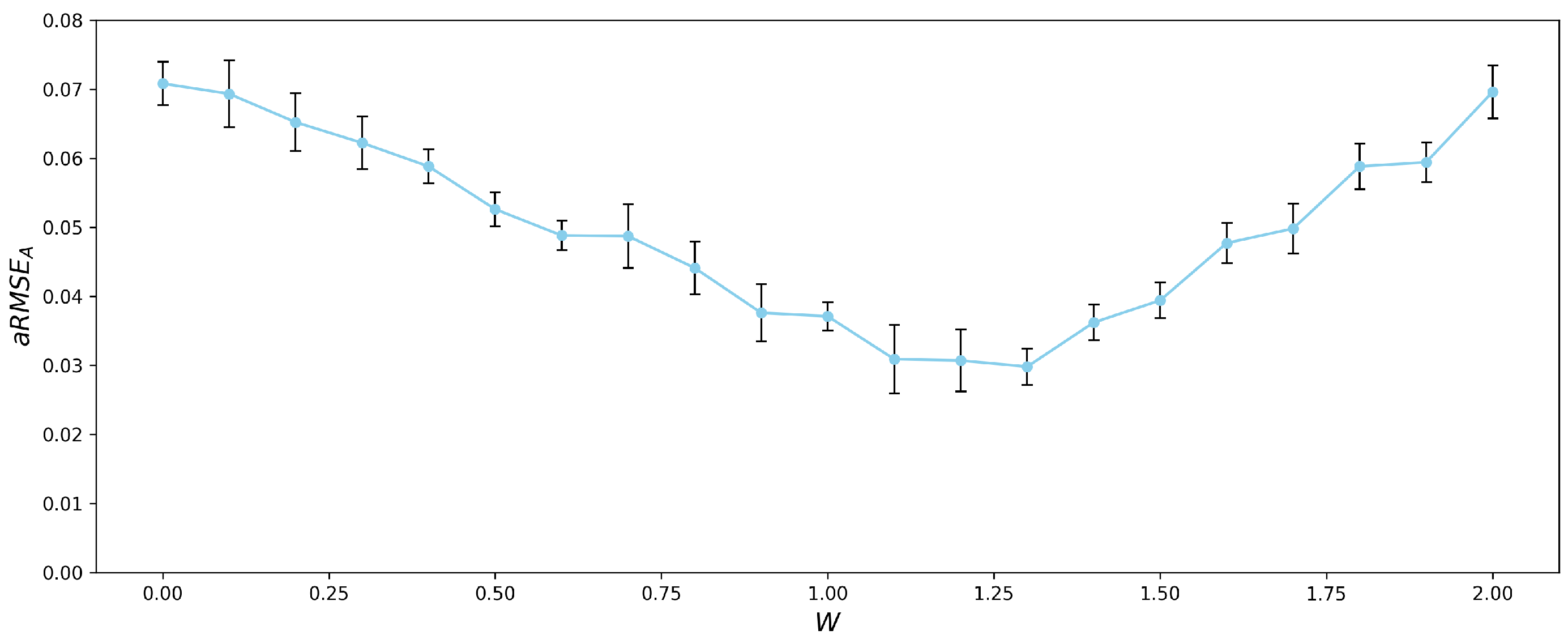
A key hyperparameter in the proposed SVCDM is the classifier-free guidance (CFG) coefficient w, which controls the trade-off between class consistency and endmember diversity. A larger value of w emphasizes the influence of class-conditional guidance, thereby improving the alignment between the endmembers and their respective classes. Conversely, a smaller value of w enhances the model’s flexibility, promoting greater endmember diversity. To further investigate the impact of this parameter, w is varied within the range of [0, 2], with an interval of 0.1. The corresponding aRMSE for each setting of w is shown in Figure 2; the lowest aRMSE of 0.03 is achieved when w is set to 1.3.

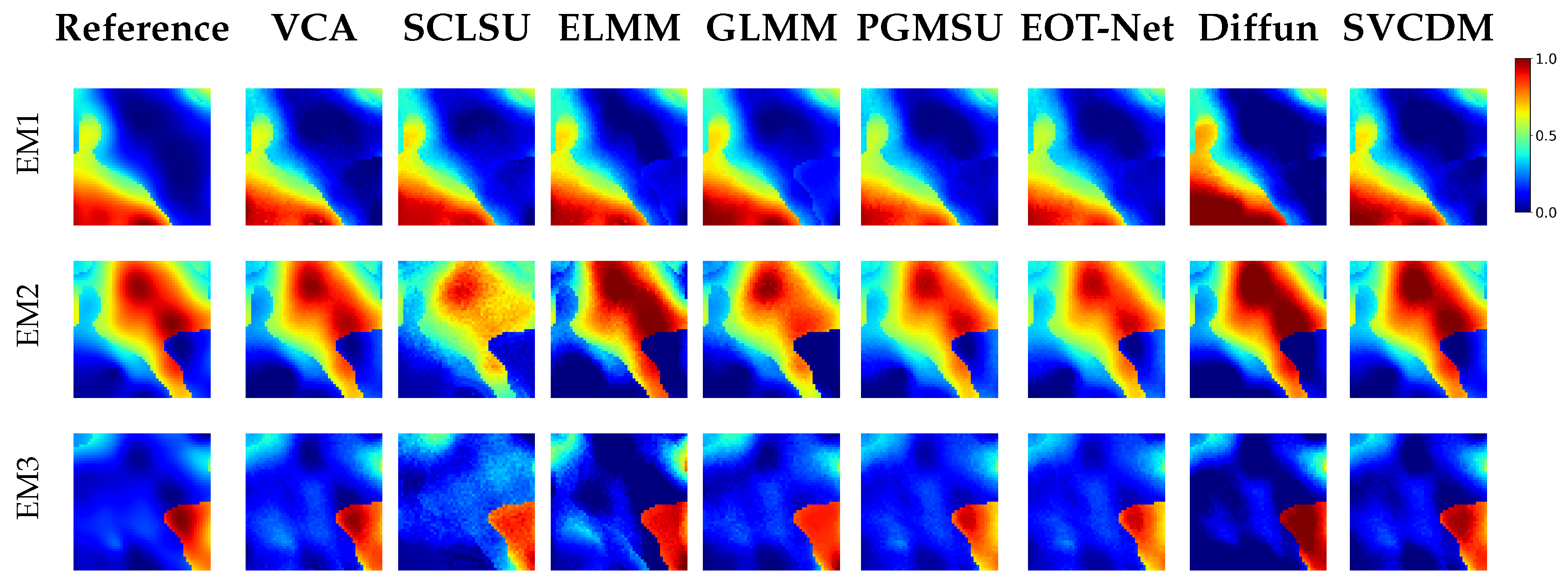
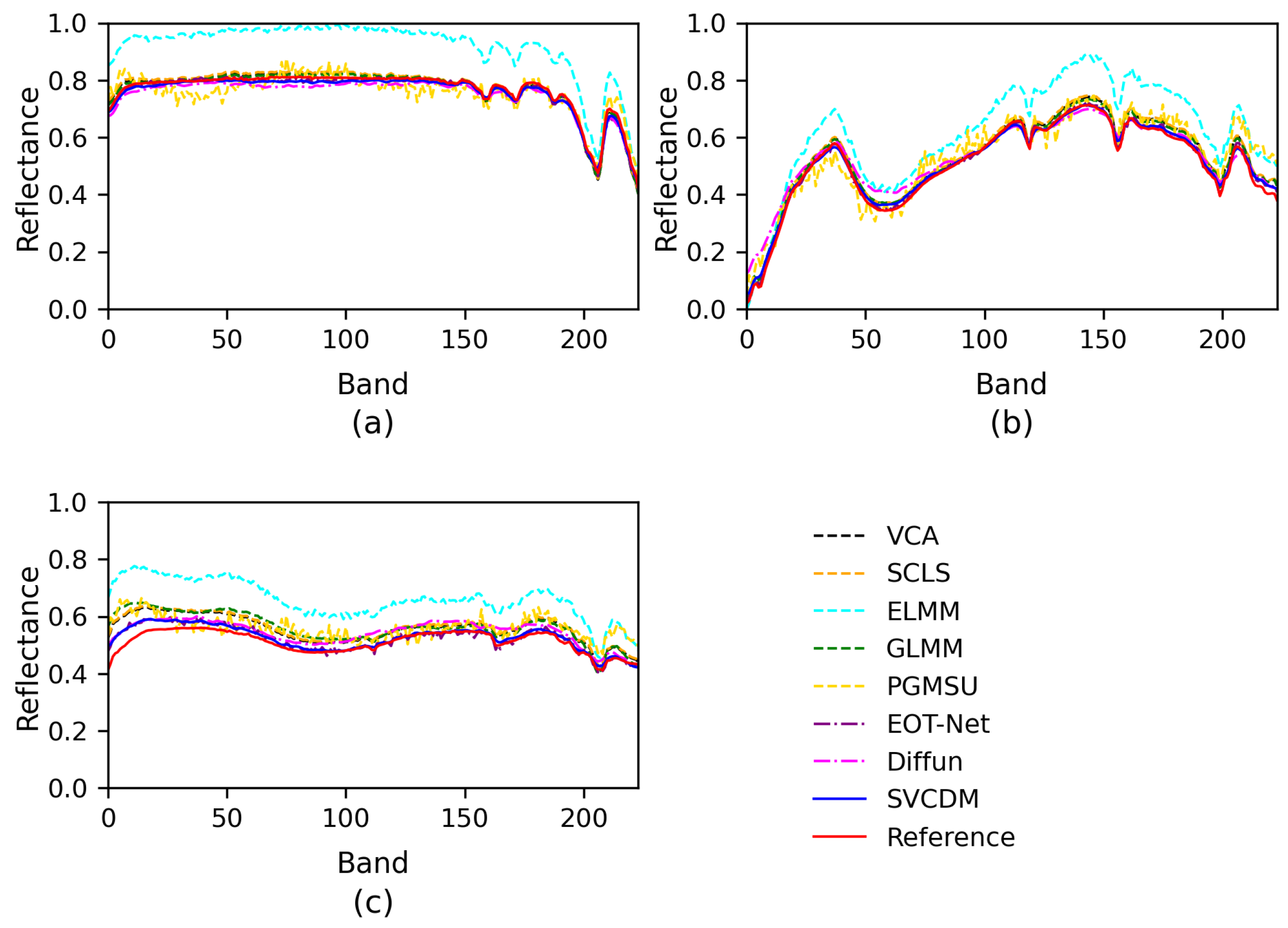
(1) Results and Discussion: 

Table 1. Comparison of evaluation metrics on synthetic datasets with Gaussian noise varying from SNR = 10 to 30 dB.

SNR = 30 dB
Methods	SAM	aRMSE	rRMSE
VCA	0.0343	0.0828	0.0351
SCLSU	0.0239	0.0794	0.0348
ELMM	0.0223	0.0737	0.0251
GLMM	0.0303	0.0574	0.0229
PGMSU	0.0474	0.0991	0.0268
EOT-Net	0.0416	0.0942	0.0259
Diffun	0.1745	0.0708	0.1688
SVCDM	0.0202	0.0371	0.0236
SNR = 20 dB
Methods	SAM	aRMSE	rRMSE
VCA	0.0484	0.0988	0.0657
SCLSU	0.0273	0.0903	0.0692
ELMM	0.0256	0.0579	0.0662
GLMM	0.0329	0.0657	0.0653
PGMSU	0.1382	0.0828	0.0661
EOT-Net	0.0915	0.0869	0.0678
Diffun	0.1721	0.0666	0.0664
SVCDM	0.0227	0.0416	0.0658
SNR = 10 dB
Methods	SAM	aRMSE	rRMSE
VCA	0.0767	0.1681	0.2206
SCLSU	0.0745	0.2526	0.2248
ELMM	0.0727	0.2045	0.2221
GLMM	0.0432	0.1391	0.2055
PGMSU	0.1961	0.0828	0.2344
EOT-Net	0.1627	0.0894	0.2291
Diffun	0.1727	0.0827	0.2046
SVCDM	0.0263	0.0797	0.2043

presents a quantitative evaluation on the synthetic dataset, using three evaluation metrics: SAM for endmember extraction, aRMSE for abundance optimization, and rRMSE at the pixel level, and the minimum values are highlighted in bold. Figure 3 and Figure 4 display the abundance maps and the corresponding endmembers extracted by various methods. Among the methods, VCA shows inferior performance across all metrics, primarily due to its sensitivity to random projections, noise, and outliers during endmember extraction, which ultimately reduces the accuracy of hyperspectral unmixing. SCLSU, while enforcing ANC and ASC to promote spatial smoothness, lacks proper regularization, resulting in suboptimal abundance estimates. In contrast, ELMM relaxes the rigid simplex assumption in a more flexible manner and incorporates regularization terms, leading to more feasible results in terms of aRMSE and rRMSE. Moreover, GLMM introduces band-wise scaling factors for each endmember, allowing for improved HSI reconstruction. Diffun demonstrates an ability to model SV but struggles to maintain class consistency of the endmembers, leading to inferior performance, especially in terms of SAM. In comparison, the proposed SVCDM achieves superior unmixing performance, with SAM and aRMSE outperforming all other methods. Although its rRMSE is slightly higher than that of GLMM, the minimal reconstruction error does not necessarily indicate inaccurate abundance estimates, thus confirming the superiority of the SVCDM on the synthetic dataset.

(2) Robustness to Noise: To assess the robustness of different methods under varying noise levels, Gaussian noise with SNRs of 30 dB, 20 dB, and 10 dB was added to the synthetic dataset. The quantitative evaluation under different SNRs is summarized in Table 1. As the SNR decreases, unmixing performance declines across all methods to varying extents, highlighting the significant impact of noise on both endmember extraction and abundance optimization. Traditional methods, such as VCA and SCLSU, exhibit a sharp degradation in performance under high noise levels, especially at 10 dB, both their aRMSE and rRMSE increase substantially. EOT-Net shows relatively better performance in terms of aRMSE but is more sensitive to noise in terms of SAM and rRMSE. Diffun outperforms most methods at 30 dB and 20 dB; however, its aRMSE increases notably to 0.0827 at 10 dB, accompanied by a rise in rRMSE to 0.2046, suggesting limited stability under severe noise. In contrast, the proposed SVCDM demonstrates superior noise robustness across all noise levels, achieving the lowest SAM values of 0.0202, 0.0227, and 0.0263, and the lowest aRMSE values of 0.0371, 0.0416 and 0.0797 at SNRs of 30 dB, 20 dB and 10 dB, respectively. Even under the most challenging noise, the rRMSE remains relatively low, underscoring the strong resilience of the SVCDM to noise.

4.3. Experiments on Real Datasets

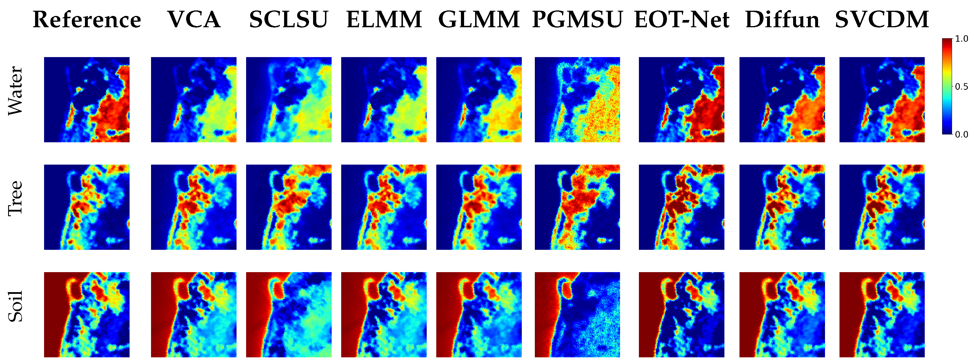
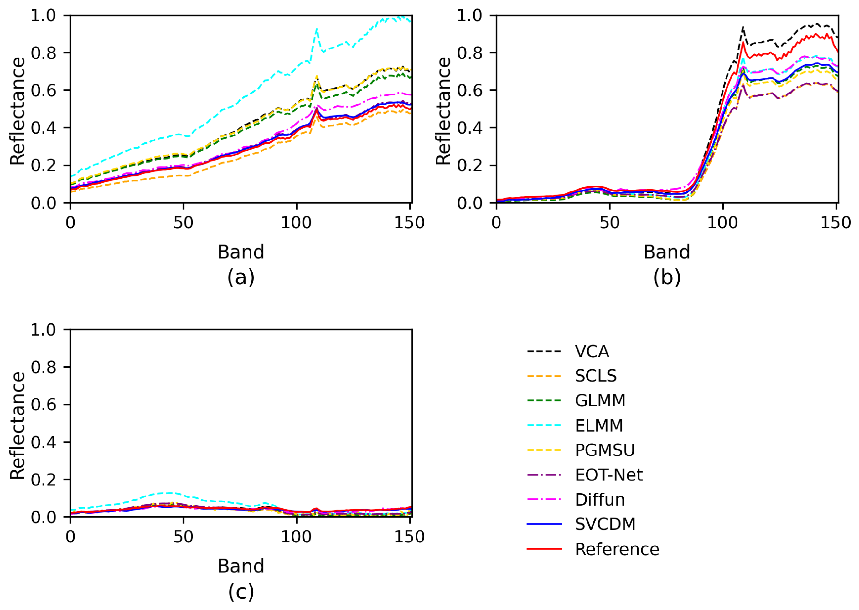
(1) Samson dataset: The original image of the Samson dataset has a size of 952 × 952, a number of bands of 156, a spectral range of 401–889 $\mathrm{n}$$\mathrm{m}$, and a spectral resolution of 3.13 $\mathrm{n}$$\mathrm{m}$. In order to reduce the computational effort, a 95 × 95 region is selected starting from (252, 332) for the experiment. This area contains three main types of objects: soil, trees and water. The pure pixels were selected as reference endmembers through manual analysis, and their abundance maps were optimized under the linear assumption to be used as benchmarks for the subsequent evaluations.

The abundance maps and the corresponding endmembers are illustrated in Figure 5 and Figure 6. The first column shows the reference abundance maps, while the remaining columns display the results obtained from different methods. The class-wise results show that the SVCDM achieves SAM values of 0.0127, 0.0171 and 0.0629, and corresponding aRMSE values of 0.0412, 0.0478 and 0.0562 for soil, trees and water, respectively. It can be observed that both VCA and ELMM exhibit significant deficiencies in the abundance maps for the soil class. Specifically, these methods produce poorly defined abundance maps, accompanied by local misclassifications, which indicates their limitations in effectively modeling SV. These observations are further corroborated by the evaluation metrics presented in

Table 2. Comparison of evaluation metrics on the Samson dataset.

Methods	SAM	aRMSE	rRMSE
VCA	0.1890	0.1212	0.0149
SCLSU	0.1983	0.1839	0.0603
ELMM	0.1816	0.1194	0.0209
GLMM	0.1964	0.1073	0.0203
PGMSU	0.0474	0.0909	0.0272
EOT-Net	0.0732	0.1664	0.0751
Diffun	0.0518	0.0502	0.1248
SVCDM	0.0309	0.0484	0.1236

, with the minimum values highlighted in bold. Although VCA achieves an rRMSE of 0.0143, its aRMSE is considerably higher than other methods, which compromises its ability to accurately optimize the abundance maps. This is largely because VCA adopts reconstruction error as the object function and introduces a substantial number of auxiliary parameters to fit the reconstruction error. In contrast, the SVCDM consistently outperforms all other methods, achieving the lowest values in both SAM and aRMSE (less than 0.05). This highlights the superior performance of SVCDM in terms of both endmember extraction and abundance optimization.

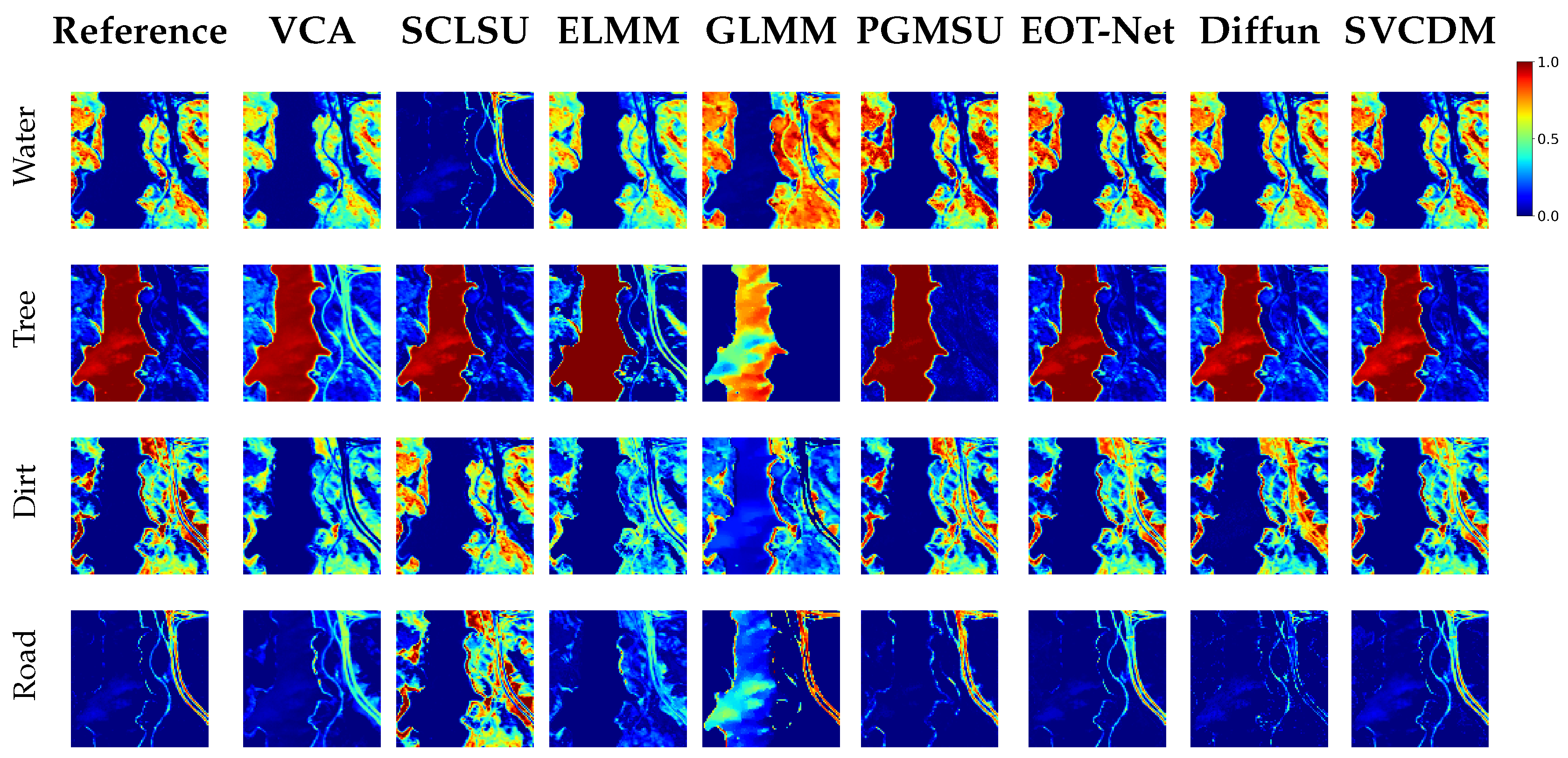
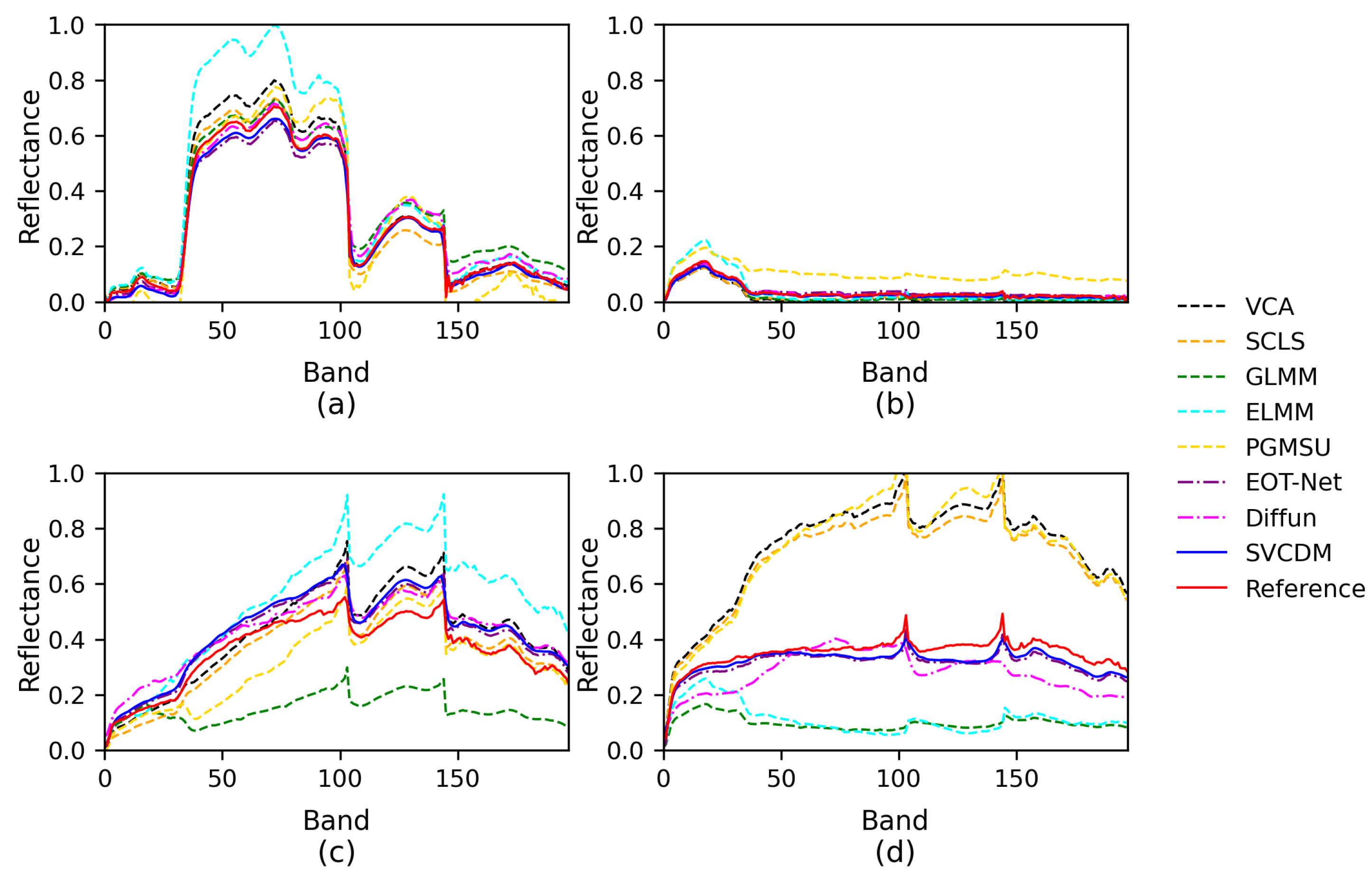
(2) Jasper Ridge dataset: Jasper Ridge is a widely used HSI dataset with a size of 512 × 614, covering 224 bands from 380 $\mathrm{n}$$\mathrm{m}$ to 2500 $\mathrm{n}$$\mathrm{m}$, and a spectral resolution of 9.46 $\mathrm{n}$$\mathrm{m}$. In our experiments, the central region of 100 × 100 pixels was selected, bands that are seriously affected by water absorption and atmosphere (1–3, 108–112, 154–166 and 220–224) were removed, and 198 bands were retained for hyperspectral unmixing. The dataset contains four main objects: dirt, soil, water and road. Similarly, the pure pixels were selected from the original HSI to construct the reference endmembers, and the corresponding abundance maps were optimized under the linear assumption.

Figure 7 and Figure 8 demonstrate abundance maps and corresponding endmembers of different methods. The class-wise results show that the SVCDM achieves SAM values of 0.0467, 0.0696, 0.0326 and 0.0514, and corresponding aRMSE values of 0.0382, 0.0445, 0.0479 and 0.0566 for tree, water, soil and road, respectively. Among these, VCA exhibits clear boundary distortions and shows limitations in accurately estimating the abundance map for water. ELMM and GLMM, which rely on parametric spectral modeling, struggle to effectively model complex SV, resulting in inaccurate endmember extraction for certain classes. Specifically, the abundance maps produced by GLMM exhibit fuzzy boundaries and unreasonably high abundance values. While PGMSU adopts a probabilistic generative framework to model the relationship between reference and extracted endmembers, the abundance maps reveal significant misclassification between soil and water.

Table 3. Comparison of evaluation metrics on the Jasper Ridge dataset.

Methods	SAM	aRMSE	rRMSE
VCA	0.1133	0.1184	0.0426
SCLSU	0.1584	0.1305	0.0547
ELMM	0.2002	0.1309	0.0216
GLMM	0.2226	0.2370	0.0285
PGMSU	0.0626	0.0481	0.0221
EOT-Net	0.0622	0.0891	0.0444
Diffun	0.1086	0.0951	0.2265
SVCDM	0.0505	0.0468	0.2263

presents the evaluation metrics for the SVCDM and all comparative methods, with the minimum values highlighted in bold. In contrast, the SVCDM demonstrates superior capability in modeling EV and produces reasonable abundance maps, particularly excelling in preserving clearer boundaries between classes.

(3) Houston dataset: This image was acquired over the campus of the University of Houston, TX, USA, in June 2012, and originally published in the 2013 IEEE GRSS data fusion competition. The original image has a size of 349 × 1905, contains 144 bands, and covers a range of 0.364–1.046 $\mathsf{\mu }$$\mathrm{m}$. In this experiment, one of the sub-images was selected, with a size of 170 × 170, containing four main objects: parking lot1, parking lot2, running track and grass healthy [60]. The pure pixels were selected from the original HSI, and the abundance maps were optimized under the linear assumption.

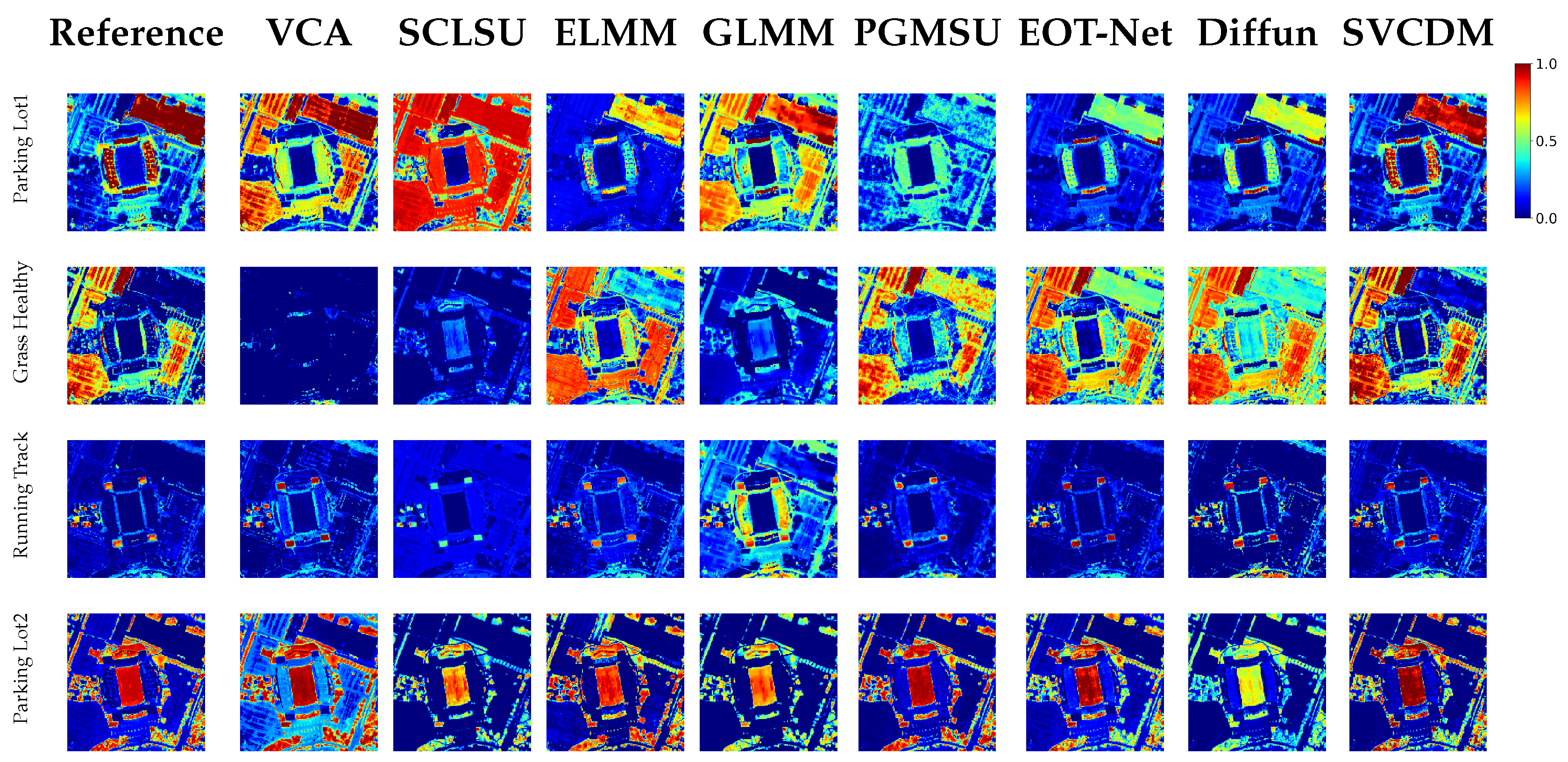
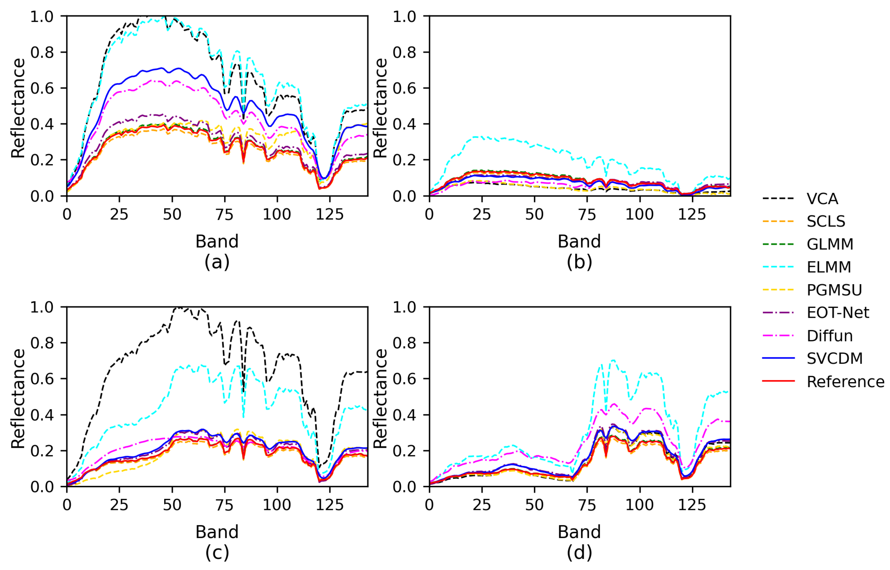
The abundance maps and corresponding endmembers of different methods are presented in Figure 9 and Figure 10. For a more detailed evaluation, the class-wise results show that the SVCDM achieves SAM values of 0.0414, 0.0441, 0.0551 and 0.0537, and corresponding aRMSE values of 0.0725, 0.0786, 0.0962 and 0.0863 for parking lot1, parking lot2, running track and grass healthy, respectively. It is evident that VCA struggles to distinguish between parking lot 1 and parking lot 2, leading to blurred boundaries between these classes. While GLMM achieves lower values of rRMSE, its abundance maps exhibit a clear estimation bias, with indistinct boundaries observed in several regions. In contrast, the SVCDM demonstrates superior accuracy in differentiating spectrally similar classes, particularly at the boundary between parking lot 1 and parking lot 2. The evaluation metrics for all comparative methods are summarized in

Table 4. Comparison of evaluation metrics on the Houston dataset.

Methods	SAM	aRMSE	rRMSE
VCA	0.1522	0.1052	0.0464
SCLSU	0.1468	0.2874	0.0947
ELMM	0.1553	0.1029	0.0392
GLMM	0.1115	0.3026	0.0736
PGMSU	0.0525	0.0867	0.1054
EOT-Net	0.0521	0.1986	0.0691
Diffun	0.1208	0.1878	0.1112
SVCDM	0.0486	0.0834	0.1134

, with the minimum values highlighted in bold. Although the rRMSE of the SVCDM (0.1134) is slightly higher than that of GLMM, the reconstruction-driven bias observed in these method—where reconstruction error is treated as the primary objective—highlights a key limitation. By incorporating conditional information into the reverse process, the SVCDM mitigates the bias introduced by reconstruction-error-driven optimization, ultimately resulting in more robust and accurate unmixing performance.

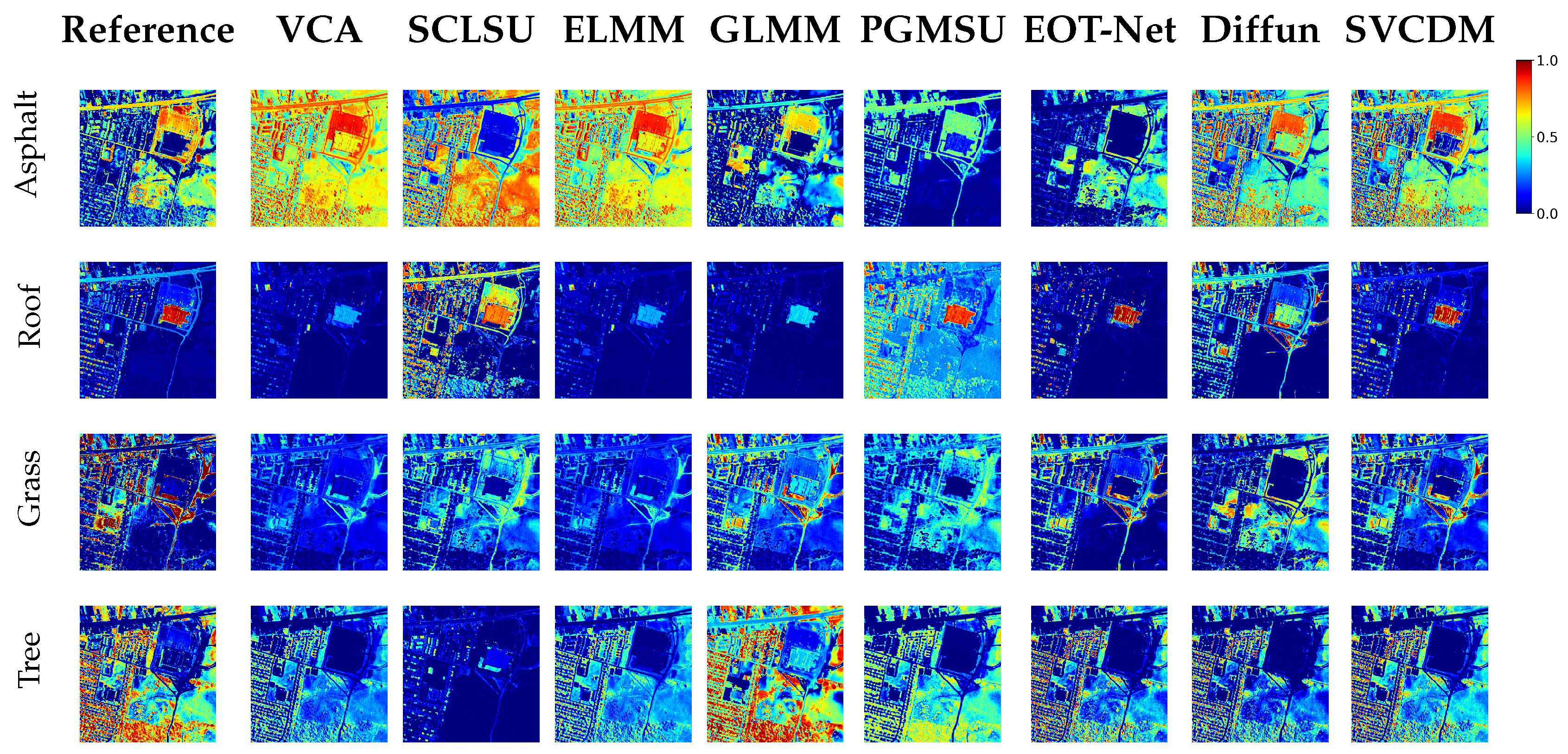
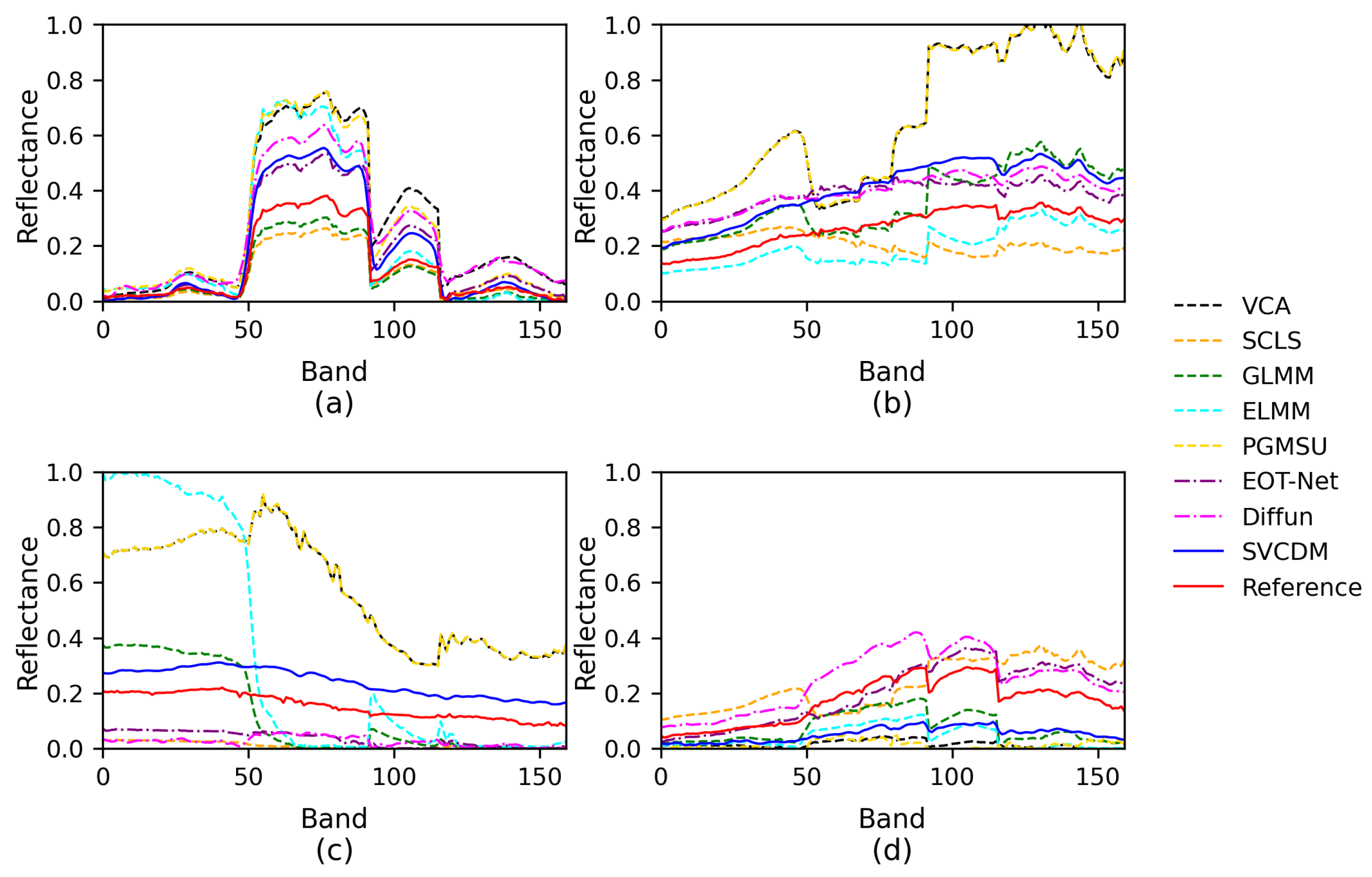
(4) Urban dataset: Urban is a classical HSI dataset in the field of hyperspectral unmixing, with 210 bands covering wavelengths from 400 $\mathrm{n}$$\mathrm{m}$ to 2500 $\mathrm{n}$$\mathrm{m}$ and a spectral resolution of 10 $\mathrm{n}$$\mathrm{m}$. Among them, bands 1–4, 76, 87, 101–111, 136–153 and 198–210 were removed to maintain a sufficient SNR, and we finally retained 162 bands for spectral unmixing. The image has a size of 307 × 307 and contains four objects: asphalt, grass, tree and roof. Moreover, four reference endmembers were selected for the experiment, and the abundance maps were optimized under the linear assumption.

Figure 11 and Figure 12 present the abundance maps and corresponding endmembers of various methods. For a more detailed evaluation, the class-wise results show that the SVCDM achieves SAM values of 0.0765, 0.0211, 0.0971 and 0.0841, and corresponding aRMSE values of 0.1667, 0.1482, 0.2004 and 0.1839 for tree, asphalt, roof and grass, respectively. Diffun demonstrates limitations in both endmember diversity and representativeness due to the absence of conditional information, resulting in less discriminative abundance maps that fail to differentiate between distinct classes. In contrast, the SVCDM preserves the boundaries between different objects more effectively and suppresses confusion between spectrally similar classes, such as roof and asphalt.

Table 5. Comparison of evaluation metrics on the Urban dataset.

Methods	SAM	aRMSE	rRMSE
VCA	0.1398	0.2647	0.1511
SCLSU	0.2426	0.2543	0.1924
ELMM	0.2376	0.2965	0.1274
GLMM	0.3402	0.1979	0.1163
PGMSU	0.1912	0.2454	0.1271
EOT-Net	0.2088	0.2714	0.0805
Diffun	0.1657	0.2747	0.1263
SVCDM	0.0514	0.1748	0.1270

summarizes the evaluation metrics for the SVCDM and all comparative methods, with minimum values highlighted in bold. Although the rRMSE of the SVCDM is 0.1270, slightly higher than that of EOT-Net, its SAM and aRMSE values are 0.1748 and 0.0514, respectively. These results indicate that a lower reconstruction error does not necessarily correlate with better abundance optimization, as it may simply reflect a closer fit between the reconstructed and original HSIs, without improving the physical accuracy of the endmembers or the discriminative quality of the abundance maps. While EOT-Net achieves the lowest reconstruction error among all methods, it suffers from reconstruction bias, where excessive emphasis on minimizing reconstruction error leads to less physically consistent endmembers. In contrast, the SVCDM incorporates appropriate conditional information during the reverse process, which slightly increases the reconstruction error but significantly improves the physical meaning of the endmembers and the discrimination of the abundance maps. This leads to more realistic and reliable unmixing performance.

4.4. Ablation Studies

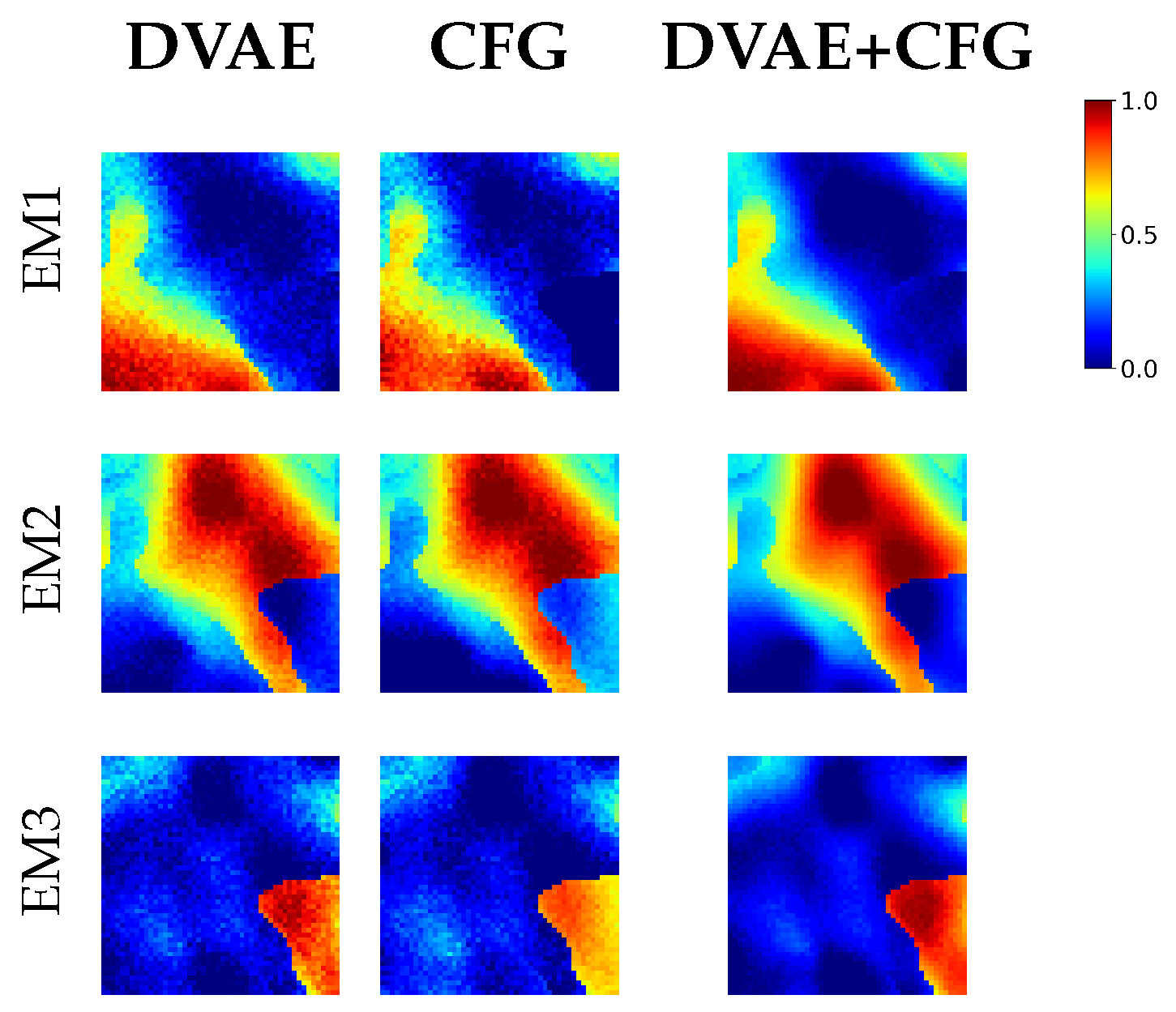
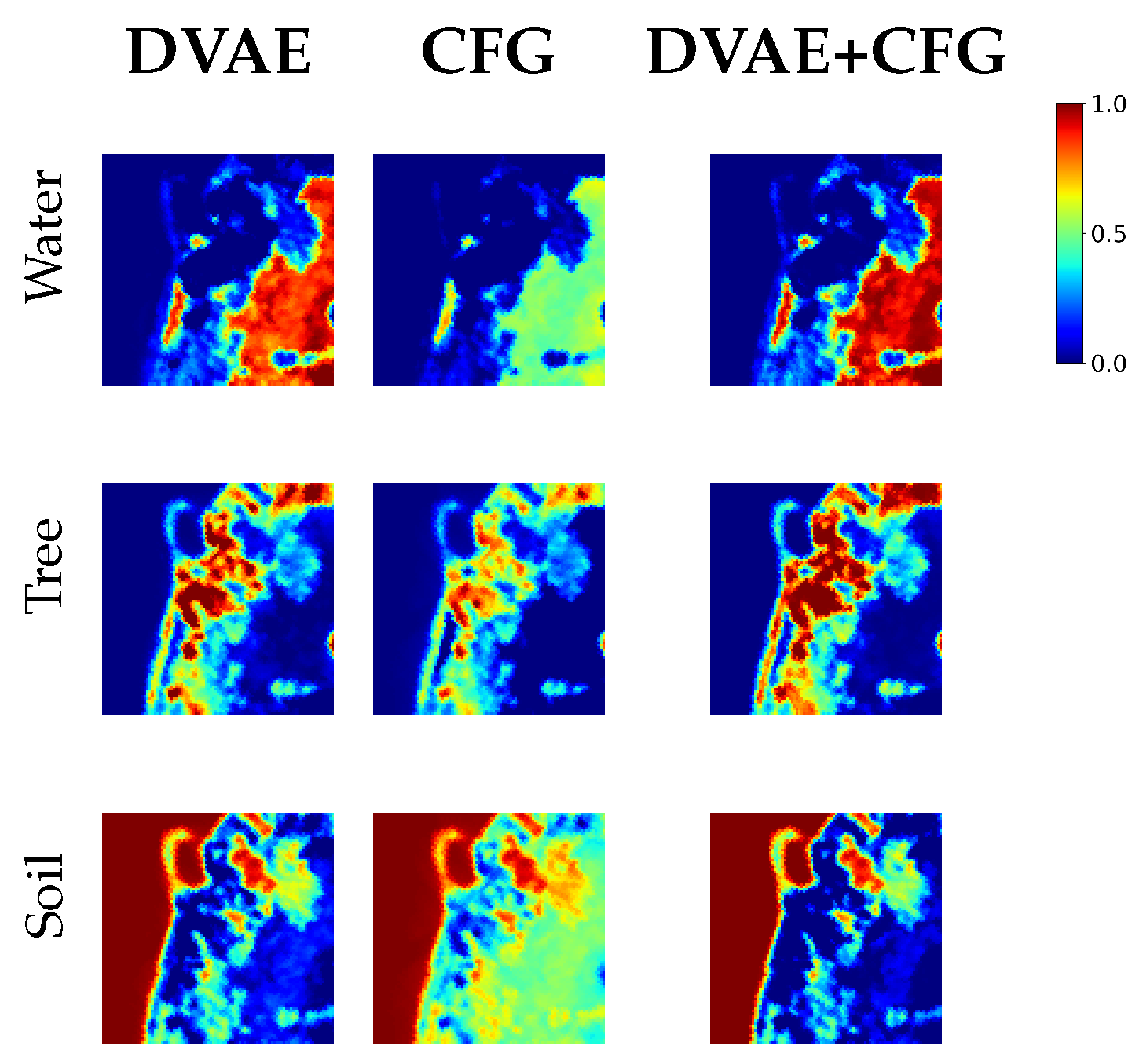
To evaluate the contributions of the DVAE and CFG modules, an ablation study was conducted, as summarized in

Table 6. Ablation analysis of the proposed SVCDM with Dirichlet distribution and CFG on the synthetic dataset with Gaussian noise of SNR = 30 dB.

Module		SAM			Mean SAM	aRMSE
DVAE	CFG	EM1	EM2	EM3
N	N	0.1098	0.0417	0.0864	0.0793	0.0915
Y	N	0.0295	0.0246	0.0318	0.0286	0.0438
N	Y	0.0469	0.0228	0.0572	0.0423	0.0614
Y	Y	0.0212	0.0207	0.0189	0.0202	0.0371

and

Table 7. Ablation analysis of the proposed SVCDM with Dirichlet distribution and CFG on the Samson dataset.

Module		SAM			Mean SAM	aRMSE
DVAE	CFG	Water	Tree	Soil
N	N	0.4049	0.0461	0.1191	0.1901	0.1482
Y	N	0.0566	0.0542	0.0476	0.0528	0.0512
N	Y	0.2521	0.0343	0.0991	0.1285	0.1484
Y	Y	0.0335	0.0311	0.0281	0.0309	0.0484

and Figure 13 and Figure 14, and the minimum values are highlighted in bold. Three model variants were assessed by selectively disabling these modules while maintaining consistent hyperparameter settings to ensure fair comparison.

With the introduction of the DVAE, the abundance maps exhibit improved spatial smoothness and more coherent coverage for dominant endmembers such as soil and water. Quantitatively, incorporating the DVAE reduces the mean SAM from 0.1901 to 0.0528 on the Samson dataset compared to the baseline without either module. This improvement arises from the Dirichlet distribution, which constrains the endmembers onto a simplex and encourages globally consistent mixing proportions. However, due to the absence of CFG, the model still struggles to distinguish objects with highly similar spectral characteristics (e.g., tree vs. water), leading to misclassification of the abundance maps in spectrally similar regions.

In contrast, the introduction of CFG strengthens class-specific separability by explicitly injecting class-aware conditional information into the reverse process. This improves the structural fidelity of each endmember and yields clearer boundaries between abundance maps of different classes, and the influence of abundance maps is controllable on the synthetic dataset. However, without the stabilizing effect of DVAE and the associated simplex constraint, the abundance maps exhibit pronounced spatial instability and the abundances are confused for different objects, characterized by excessive local fluctuations, over-fragmentation and reduced overall coherence.

The combination of both the DVAE and CFG yielded the most favorable results across all evaluation metrics. Specifically, the mean SAM is further reduced to 0.0309, and the aRMSE reaches the lowest value of 0.0484 on the Samson dataset. Similar trends are also observed on the synthetic dataset, where the mean SAM is further decreased to 0.0202 and the aRMSE achieves the lowest value of 0.0371. The Dirichlet distribution regularizes the latent representations within realistic spectral bounds, while CFG improved semantic alignment and discrimination during the reverse process. This complementary interaction allows the model to better capture intrinsic SV. Overall, both components are integral to enhancing the unmixing performance of the proposed SVCDM.

4.5. Discussion

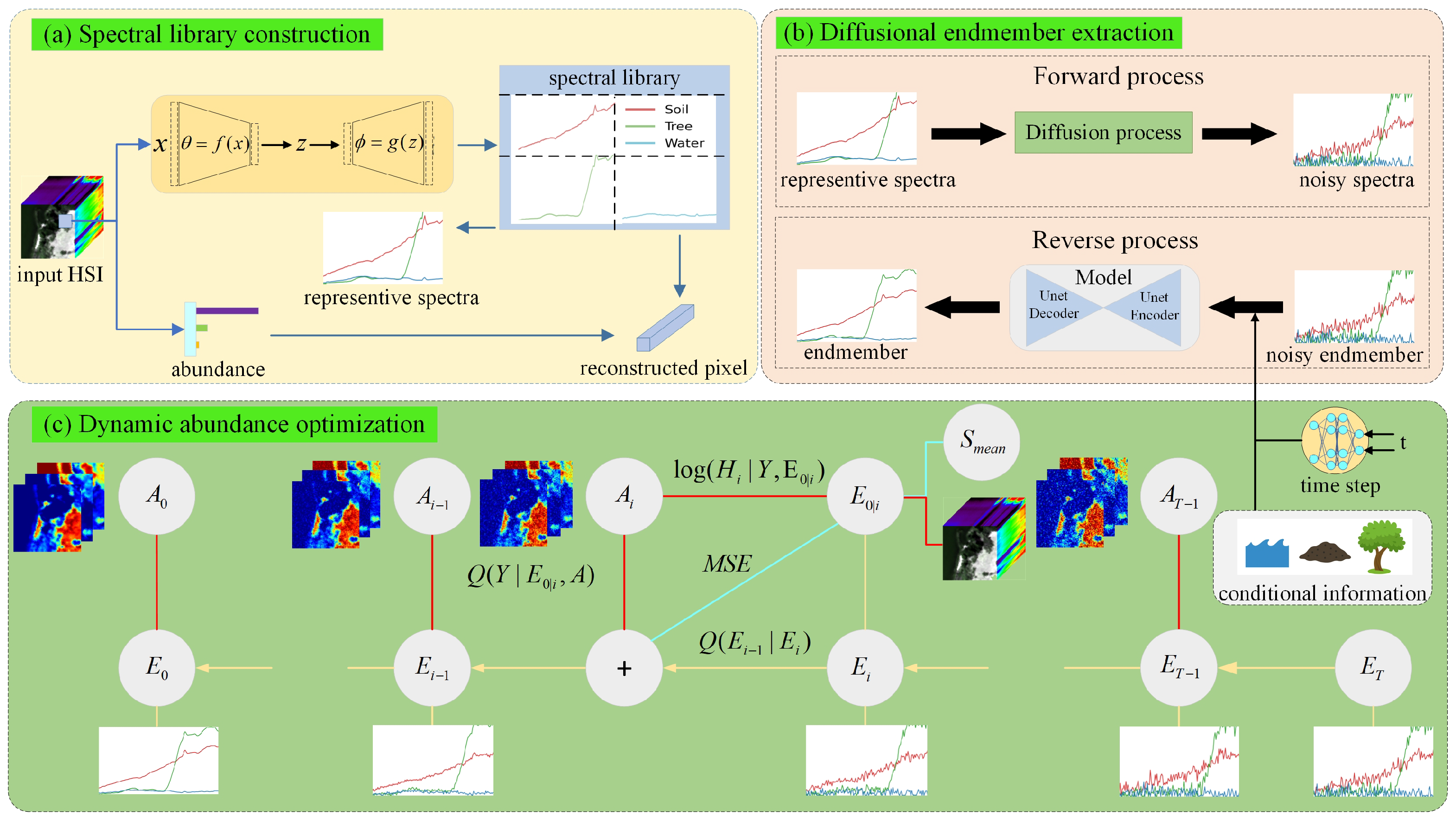
The proposed SVCDM demonstrates strong performance in hyperspectral unmixing, particularly in accurately modeling SV and incorporating class constraints into the endmember extraction. The spectral library obviously ignores the redundant spectra in the HSI, and narrows the range of endmember extraction. On the synthetic dataset, the influence of noise is slight for the SVCDM; the SAM is on the magnitude of 0.02, which is approximate to the reference endmembers; and the details of the abundance maps are close to the ground truth. On the Samson and Jasper Ridge datasets, the SVCDM is used successfully to recognize soil, tree and water, the aRMSE is less than 0.06 for all objects, and the differences in the abundance maps are subtle, compared to the reference. On the Houston and Urban datasets, the SAM values are under 0.05, with 0.0414 and 0.0441 for parking lot1 and parking lot2 respectively, which proves that the SVCDM is efficient in recognizing similar objects. Although the aRMSE is higher than 0.2 for asphalt, the corresponding value is only 0.0211, which is because the SVCDM does not explicitly optimize reconstruction error as the primary objective, but instead emphasizes physically meaningful endmember and abundance estimation, which may lead to slightly higher reconstruction errors in some cases. The SVCDM is able to generate complex prior distributions and extract physically consistent endmembers, and the use of CFG further enhances class discriminability, leading to more accurate and stable abundance maps. These advantages are consistently reflected in the experimental results, where SVCDM achieves superior performance in terms of SAM and aRMSE across synthetic and real datasets.

The SVCDM models the underlying prior distribution of endmembers, and employs iterative optimization (e.g., L-BFGS) to refine abundance optimization. This process is interpreted as a two-layer dynamic programming, which contributes to coverage to the global optimum with the increased computational overhead. Moreover, the unmixing performance of the SVCDM is influenced by several hyperparameters, such as the CFG coefficient w, which may require fine-tuning for different datasets, and thus may have limited capability in handling complex scenarios.

5. Conclusions

This paper proposes an SVCDM for unsupervised hyperspectral unmixing that designs a DVAE for constructing a spectral library with a class constraint and prior distribution and a DM with conditional information for endmember extraction with dynamic abundance optimization. The proposed method addresses the challenges of modeling complex SV in HSIs. Specifically, the class labels of the endmembers are used as conditional information to guide the DM in learning the distribution more accurately. At each time step of the reverse process, the gradient of the log-likelihood is leveraged to jointly optimize abundance maps with the endmember matrix, enhancing the abundance optimization along with the updating of endmembers.

Experimental results on both synthetic and real datasets demonstrate the superior unmixing performance of the proposed method, particularly in handling complex SV. Compared to existing approaches, the SVCDM exhibits notable advantages in accurately modeling SV. By effectively combining the generative power of the DM with the linear unmixing assumption, the method provides a novel approach for hyperspectral unmixing. In future work, we aim to extend the network to handle dynamic scenarios with time-varying characteristics and explore more sophisticated bootstrapping strategies to further enhance the unmixing performance and the ability to model SV. Additionally, hyperspectral unmixing of satellite-acquired data remains challenging, particularly over large and diverse regions. Future work will focus on developing more advanced strategies to improve scalability and robustness in real-world applications.