Sun-Induced Chlorophyll Fluorescence (SIF) Enhances Soil Respiration Estimation in Desertified Mining Areas

Highlights

What are the main findings?

• SIF improves soil respiration (Rs) inversion accuracy in desertification mining areas by 26.8%.
• The RF model outperforms other machine learning methods for Rs remote sensing inversion.

What are the implications of the main findings?

• SIF proves to be a more accurate vegetation representation factor than vegetation indices.
• SIF provides insights for understanding carbon cycle dynamics in large-scale mining areas.

Abstract

Soil respiration (Rs) is influenced by various factors, including soil temperature (ST), soil moisture (SM), and vegetation growth. Accurately and quantitatively estimating Rs from remote sensing data is essential for understanding the carbon cycle in desertification ecosystems. However, selecting appropriate vegetation representation factors poses a significant challenge during the remote sensing inversion. Sun-Induced Chlorophyll Fluorescence (SIF) is used extensively to monitor vegetation diseases and pests, assess drought conditions, and estimate Gross Primary Production (GPP). Nevertheless, the applicability of SIF for estimating Rs from remote sensing data and whether Rs modeling surpasses traditional vegetation indices requires further investigation. This study focuses on the Hongshaquan mining area, utilizing UAV hyperspectral, thermal infrared, and in situ monitoring data, combined with four machine learning methods: Random Forest (RF), Partial Least Squares (PLS), Support Vector Machine (SVM), and Back Propagation Neural Network Algorithm (BP) to establish a model for estimating Rs from remote sensing data. The determination coefficient (R²) and root mean square error (RMSE) were used to assess the performance of Rs inversion models characterized by SIF, Normalized Difference Vegetation Index (NDVI), and Near-Infrared Reflectance of Vegetation (NIRv) improved by radiance. The feasibility and modeling potential of estimating Rs from remote sensing data using SIF were explored. The results indicate that vegetation significantly impacts Rs in desertification mining area ecosystems, and the inversion accuracy of Rs improved by 26.8% after incorporating vegetation factors. The RF model displayed the best overall performance among the four machine learning methods. When the Salinity Index (SI) and Temperature Vegetation Dryness Index (TVDI) were treated as fixed components of the modeling independent variable, the modeling accuracy of the various vegetation representation factors ranked from highest to lowest as follows: SIF > NIRv > NDVI, with corresponding R² values of 0.63, 0.58, and 0.57, and RMSEs of 0.08 μmol·m⁻²·s⁻¹, 0.12 μmol·m⁻²·s⁻¹, and 0.13 μmol·m⁻²·s⁻¹, respectively. The research findings suggest that SIF holds significant promise for remote sensing estimation of Rs. The use of SIF can enhance the accuracy of Rs estimation.

1. Introduction

Soil respiration (Rs) is the second-largest flux in the ecosystem carbon cycle, contributing to 60% to 90% of total respiration in terrestrial ecosystems. Each year, soil releases 90 PgC into the atmosphere [1]. In developing countries, coal remains a primary energy source [2]. While coal mining fosters economic development, it also significantly harms ecological conditions, impacting vegetation, terrain, and soil in mining areas [3]. This damage leads to increased carbon emissions and diminishes the carbon sequestration capacity in those regions [4]. As a key component of the carbon cycle in terrestrial ecosystems, vegetation root respiration substantially affects Rs [5]. Rs in vegetated areas closely correlate with plant growth. Most existing studies have utilized optical vegetation indices (such as Normalized Difference Vegetation Index (NDVI), Enhanced Vegetation Index (EVI), Ratio Vegetation Index (RVI), etc.) for soil respiration (Rs) [6,7,8,9]. The, yet the effectiveness of solar-induced fluorescence (SIF) in Rs inversion remains uncertain. Therefore, examining the feasibility of using SIF for Rs inversion and investigating the differences between SIF and various vegetation spectral indices in remote sensing estimates of Rs can provide new insights for quantitatively monitoring Rs in mining regions and on a global scale. This research offers a solid data foundation for carbon sequestration in ecosystems and a scientific basis for regulating carbon cycling and mitigating global warming.

Researchers have conducted extensive research on the components of assertions that Rs generally involves: three organic biological processes (namely soil microbial respiration, soil animal respiration, and plant root respiration) and one inorganic chemical oxidation process, noting that soil animal respiration and the inorganic chemical oxidation process exert minimal effects on Rs. Rs includes plant root autotrophic respiration and soil microbial heterotrophic respiration. The influence of autotrophic and heterotrophic respiration on total respiration varies under different soil conditions. Subke et al. [5] indicate that in tropical regions, autotrophic respiration significantly contributes to total respiration, with a contribution rate of approximately 60%. Lee et al. [10] discovered that in the cold temperate zone of Japan, the contribution rate of autotrophic respiration to total respiration in deciduous forests varied with the seasons, with a difference of up to 44%. This phenomenon is particularly notable in desert ecosystems; Yang et al. [11] reported that the contribution rate of root respiration to the total Rs of four desert vegetation species—Sammy, Setaria, Laterica, and Artemisia Shabana—exceeded 60%, with the contribution rate of Setaria’s root respiration reaching 80%. Liu et al. [12] demonstrated that the contribution rate of autotrophic respiration in the shrubland ecosystem of the Mu Us desert fluctuated between 54% and 69% with seasonal changes. Zhou et al. [13] found that Rs intensity in desert areas varied significantly with differences in plant rhizosphere microbial abundance. In summary, autotrophic respiration is crucial for the Rs rate in desertification ecosystems, highlighting the importance of selecting vegetation factors. Furthermore, SIF directly correlates with plant photosynthetic activity, offering mechanistic insights that traditional optical vegetation indices do not provide. Consequently, this study introduces SIF to create an RS remote sensing inversion model and compares its modeling performance with that of vegetation indices. This study aims to investigate the potential and practicality of SIF in monitoring Rs, presenting innovative ideas and practical strategies for quantitatively monitoring Rs in desertification coal mine reclamation areas and natural regions.

Due to the influence of mining activities, the pattern of carbon sources and sinks in desert areas has changed dramatically because of poor natural conditions and a fragile ecological environment. Accurate measurement of Rs in desertified mining regions serves as the foundation for clarifying the carbon cycle in these areas. Currently, the in situ monitoring method is the primary approach for measuring Rs in mining locations. Mukhopadhyay et al. [14] utilized the in situ observation method to calculate the Rs rate in reclamation areas of coal mines, finding that the longer the reclamation period, the higher the Rs. Ren et al. [15] employed the in situ monitoring method to assess Rs in the Jinshaan-Meng mining area, discovering that various soil structures in reclamation areas of the dumps significantly influenced Rs. Fang et al. [16] point out that the soil carbon emissions in mining areas mainly rely on in situ monitoring methods. The research subjects were mainly focused on the reclamation ecosystems of coal mines and metal mining areas, and it was found that the emission process was dynamically changing due to the influence of mining and reclamation. Although the in situ monitoring method can accurately measure Rs, it is limited to small-scale data collection. It inevitably causes damage to soil structure, making it unsuitable for large-scale Rs estimation. With advancements in remote sensing technology, several studies have combined hyperspectral, multispectral, and related environmental factors to construct Rs remote sensing models for large-scale spatial inversion. Liu et al. [17] used the green chlorophyll vegetation index and red edge chlorophyll index to represent vegetation factors in the mining area, along with soil temperature, humidity, and salinity indices, building a machine learning remote sensing inversion model to accurately depict the spatial distribution of Rs in the Hongshaquan mining area. Cui et al. [6] integrated NDVI, EVI, and RVI with hyperspectral characteristics to create Rs inversion models, finding a higher correlation between EVI and RVI with Rs than with NDVI. Azevedo et al. [8] employed NDVI to predict Rs in the Arctic tundra, discovering a correlation of about 0.55, indicating a nonlinear relationship, suggesting that the remote sensing method predicts Rs better. Weiland et al. [9] used satellite surface temperature and soil moisture data to estimate Rs in temperate deciduous and coniferous forests in Canada through three empirical models of Rs and a Random Forest model, finding that the Random Forest model, based on satellite temperature and moisture data, could explain 70% of the variations in Rs. Huang et al. [7] utilized remote sensing data such as land surface temperature, NDVI, and EVI as independent variables, combined with three machine learning methods: Random Forest regression (RFR), Support Vector Machine regression (SVR), and artificial neural network (ANN), to invert global Rs changes. They discovered that land cover changes significantly influenced the regulation of Rs in temperate and cold zones during 2000–2014. Rs frequently and significantly fluctuated in areas with low vegetation cover (vegetation height less than 5 m). Currently, the vegetation representation factors used in existing studies are dimensionless spectral indices, such as NDVI, EVI, and RVI. Simultaneously, few studies on Rs incorporate mechanistic parameters that can directly reflect actual photosynthetic activities of plants (such as SIF, etc.). Although SIF has made significant strides in remote sensing of the carbon cycle [18,19,20] and vegetation stress [21,22,23], it remains unclear whether it can be utilized for quantitative inversion of Rs and whether its modeling performance surpasses that of traditional vegetation indices, and its direct link to root autotrophic respiration (via photosynthetic substrates) has not been exploited for Rs modeling.

This study focuses on the Hongshaquan open-pit coal mine as the research area, utilizing Unmanned Aerial Vehicle (UAV) hyperspectral data, in situ monitoring Rs data, and temperature and humidity data to explore the potential of SIF for quantitatively estimating Rs from remote sensing data through remote sensing, and it compares this with traditional optical vegetation indices. We developed the optimal remote sensing inversion model for Rs to reveal the spatial distribution of soil carbon emissions in desert mining ecosystems, providing a scientific method for non-destructive detection to accurately estimate the carbon cycle of desert ecosystems. This offers essential data and a scientific basis for land reclamation in desertified mining areas and the sustainable development of mining areas in line with the “carbon peaking and carbon neutrality” policy.

2. Materials and Methods

2.1. Study Area

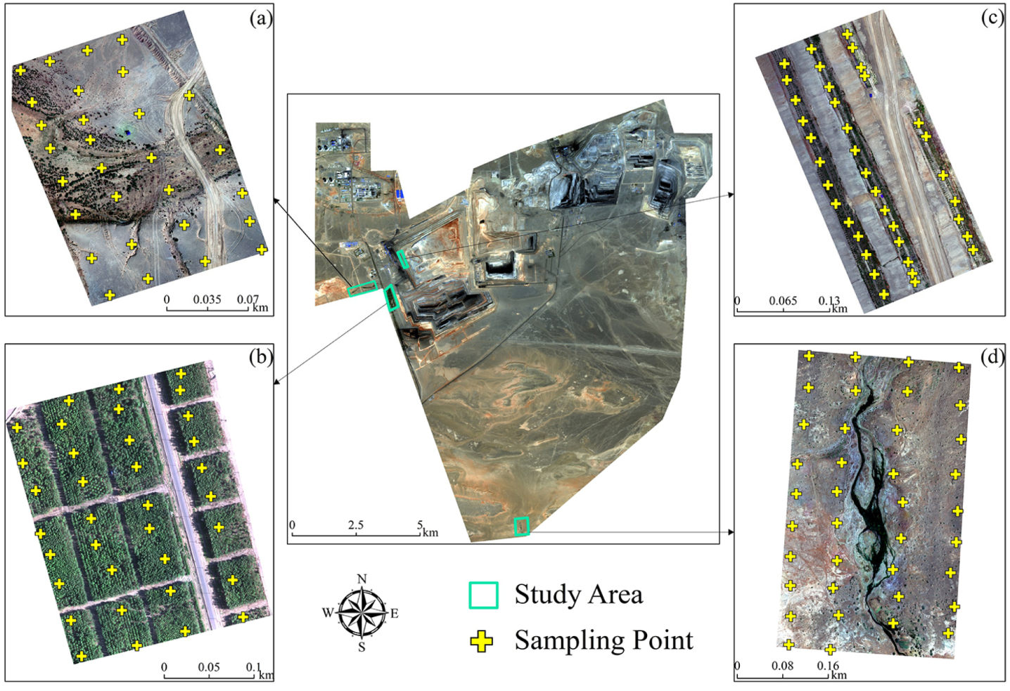
The Hongshaquan mining area is located 78 km north of Qitai County in Changji Prefecture, Xinjiang Uygur Autonomous Region, China (Figure 1), with coordinates approximately at 90.25°E to 90.42°E and 44.41°N to 44.52°N, and has an elevation ranging from 657 to 753 m. The climate in the mining area is dry and windy, characterized by low rainfall, significant evaporation, and abundant sunshine, typical of the arid climate found in continental deserts. The average annual precipitation is around 106 mm, while the annual evaporation ranges from 1200 to 2400 mm, with an average annual temperature of 5.5 °C. Both annual and diurnal temperature variations are considerable [24]. The soil in the study area contains over 85% gravel (particle size 2 to 0.2 mm). According to international classification standards [25], the soil is classified as sandy soil. The pH level of the soil exceeds 7, indicating its alkalinity. Surface vegetation is sparse, with coverage between 3% and 5%. The vegetation type is uniform, sparse, and low; the community and ecosystem structures are fragile, with the leading dominant species including Salicornia europaea, Haloxylon ammodendron, and Alhagi sparsifolia, among others. On the west side of the mine, there is a dry riverbed extending from southwest to northeast, featuring low-growing vegetation primarily composed of Tamarisk (Figure 1a). Within the mining area, there are two reclamation sites: a plantation (Figure 1b) and a waste dump (Figure 1c). A spring located 10 km from the southern end of the mining area (Figure 1d) serves as the source of northward runoff. After approximately 800 m of runoff, the water percolates or evaporates at the endpoint [26].

2.2. Theoretical Basis for Inversion of Soil Respiration by SIF

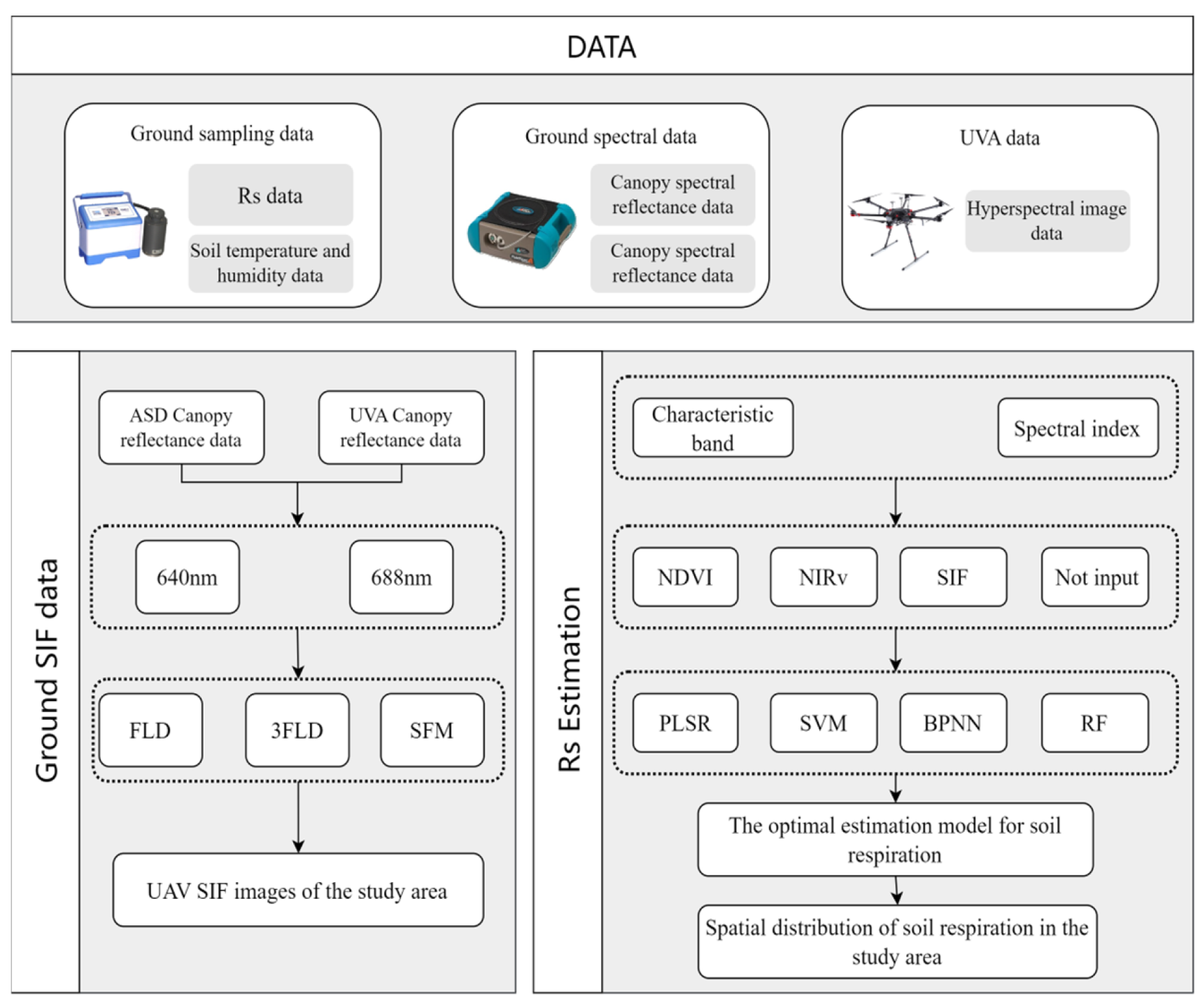
Rs mainly comprises autotrophic respiration (Ra) and heterotrophic respiration (Rh). Ra pertains to the respiratory process of plant roots that produce CO₂ from substrates arising from photosynthesized products distributed by plants to the soil. Besides temperature and humidity, the rate of Rs is also influenced by the photosynthetic status of plants. In contrast, Rh is the result of CO₂ released during the decomposition of organic matter by soil microorganisms, predominantly affected by soil temperature and moisture [27]. Studies indicate that in desert ecosystems, plant Ra constitutes a significant portion (40–80%) of total Rs [11,12]. Hence, understanding the influence of desert vegetation is crucial for accurately monitoring the spatial distribution of Rs in arid regions and further investigating the ecosystem’s carbon cycle. From a remote sensing perspective, a stronger correlation between factors representing vegetation and GPP suggests a more accurate reflection of changes in vegetation’s physiological activities [19]. Current studies commonly use NDVI to characterize vegetation, although some also utilize chlorophyll-related spectral indices, such as the green chlorophyll vegetation index (CI_green) and the red-edge chlorophyll vegetation index (CI_red-edge). Nonetheless, these indices are scalar values based on reflectance and lack comprehensive insights into photosynthetic processes. When coupled with machine learning techniques, these parameters can lead to improved inversion results, but lack mechanistic explanations during the process. SIF represents the spectral signal emitted by plants under sunlight, encapsulating quantitative information regarding their photosynthetic activity. This correlation is why SIF aligns more closely with GPP than other vegetation indices [28,29]. The photosynthetic substrates that plants transport to their roots form the basis for root respiration. These substrates that influence root respiration are components of GPP, which is also closely associated with SIF (Figure 2). Can SIF be utilized to create a remote sensing model for Rs that produces more reliable outcomes? To assess the feasibility and potential of SIF for estimating soil respiration, this study evaluated the accuracy of soil respiration estimation models developed with three different vegetation factors: NDVI, NIRv, and SIF. Additionally, the varying performance of these factors in estimating soil respiration was illustrated via model accuracy. The technical roadmap for this study is presented in Figure 2.

2.3. Data Collection

2.3.1. Local Data

The soil respiration rate of surface soil in four areas of the Hongshaquan open-pit mining site was determined using an EGM-5 portable infrared gas analyzer (PP-Systems, Amesbury, MA, USA), with 137 sample points measured (

Table 1. Distribution of the number of sampling points.

Experimental Plot (Management Type)	Dump Reclamation Area (Microbial Reclamation)	Plantation Forest (Traditional Reclamation)	Tamarix Forest (Natural Drought)	Hongsha Spring (Natural Drought)
sampling number	36	35	29	37

). Measurements were conducted from 10:00 to 15:00, and the respiration rings were buried at the corresponding points one to two days in advance to minimize errors caused by soil structure damage during the rings’ burial. Once the rings were buried, their positions remained unchanged. Each sampling with the instrument lasted 100 s, and the soil respiration rate at each point was measured three times, with the average value recorded as the respiration rate for that sample point. The soil carbon flux measurement system, which included the STP-2 Soil Temperature Probe, SRC-2 Soil Respiration Chamber, and EGM-5 (PP-Systems, Amesbury, MA, USA) soil carbon flux host, collected data on the soil respiration rate and recorded changes in soil temperature at that time. A PR2 profile probe (British PR2) measured the soil moisture content at the sample points. The exact coordinates of the sampling points were obtained using the Stone S10 GPS-RTK (Stone, Guangzhou, China). The spectrum of the vegetation canopy was collected using the ASD FieldSpec 4 (Analytical Spectral Devices [ASD] Inc., Boulder, CO, USA) between 13:00 and 13:30. During this period, the probe was suspended approximately 50 cm above the canopy to ensure no shadow affected the collection area. Ten spectral curves were obtained for each canopy, and the arithmetic mean was calculated as the corrected pure spectral curve of the canopy after adjusting for the jump point.

2.3.2. UAV Data

The hyperspectral image data for the study area were acquired using the PikaL hyperspectral imager (Resonon, Bozeman, MT, USA) mounted on the DJI Jingwei M600Pro RTK UAV (DJI, Shenzhen, China). The spectrometer’s spectral range extended from 400 to 1000 nm, with a spectral resolution of approximately 4 nm. The imaging spectrometer’s field of view (FOV) was set to 25°, and the flight altitude was established at 120 m according to the pre-planned route. The heading and side overlap were configured to 75% and 80%, respectively, while the radiation was calibrated using reflective gray cloth. MegaCube 2.7.0 and ENVI 5.3 software were utilized to process the original UAV data, yielding hyperspectral radiance and reflectance image data with 150 bands, each with pixel sizes of 0.05 m. Given that the UAV operated close to the ground, the absorption and scattering effects of the atmosphere were disregarded. The real-time irradiance data corresponding to the flight area was obtained by extracting the mean pixel values from the gray cloth region in the radiance image using ENVI 5.3 and combining them with the standard reflectivity file of the gray cloth.

Thermal infrared and multispectral projective images of the study area were captured using the Zenmuse XT2 thermal infrared (7.5–13.5 μm) sensor and the red edge multispectral sensor on the DJI Jingwei M300 RTK drone (DJI, Shenzhen, China). The data collection occurred between 13:00 and 14:00 on the same day. The ASD-2000 spectrometer measurement calibration reflector was employed to calibrate the sensor before the flight, with the flight altitude, heading, and side overlap matching those of the hyperspectral acquisition system. The thermal infrared camera has a resolution of 0.05 °C. The spatial resolution of the acquired multispectral orthophotography data is equivalent to that of the hyperspectral image, which will be used for the geographic registration of hyperspectral data later. After collecting all the UAV image data, ArcMap 10.5 was utilized to extract pixel values at the upper sampling points of the image for subsequent feature selection, model construction, and accuracy verification.

2.4. Data Processing

2.4.1. Feature Band Selection

The feature bands for modeling were chosen through the analysis method based on the Pearson correlation coefficient. The correlation between the feature bands and the measured soil respiration was confirmed using a 99% significance test.

2.4.2. Calculate UAV SIF Data

In the band with SIF emission (650 nm~800 nm), the reflected energy of vegetation is affected by SIF, and the reflection at wavelength λ can be expressed as the following formula [30]:

$$L(\lambda )={\displaystyle \frac{\rho (\lambda )\times E(\lambda )}{\pi }}+f^{SIF}(\lambda )$$

(1)

where L(λ) represents the apparent plant radiance at wavelength λ, ρ(λ) represents the actual reflectance at wavelength λ, E(λ) represents the solar irradiance at wavelength λ, and f_SIF(λ) represents the emission SIF at wavelength λ.

Due to the sampling equipment, accurately estimating SIF in the O₂-A band (759 nm to 770 nm) is impossible, with a deviation of about ±15% of the radiation energy of the homogeneous pixel in the same field image. Therefore, in this study, the H_α band (656.1 nm to 656.5 nm) and the O₂-B band (686 nm to 688 nm) were used as inversion windows, and Fraunhofer Line Discrimination (FLD), three-band Fraunhofer Line Discrimination (3FLD), and the Spectral Fitting Method (SFM) were utilized to invert SIF.

(1)

FLD

The FLD algorithm was proposed by Plascyk and Gabriel [31]. Using the apparent radiance and irradiance of a band inside the Fraunhofer line (λ_in) and a band outside the Fraunhofer line (λ_out), brought into (1), we obtain:

$$\left\{\begin{array}{l}L({\lambda }_{in})={\displaystyle \frac{\rho ({\lambda }_{in})\times E({\lambda }_{in})}{\pi }}+f^{SIF}({\lambda }_{in})\\ L({\lambda }_{out})={\displaystyle \frac{\rho ({\lambda }_{out})\times E({\lambda }_{out})}{\pi }}+f^{SIF}({\lambda }_{out})\end{array}\right.$$

(2)

Suppose that the SIF remains constant within the inversion range, then $\rho ({\lambda }_{in})=\rho ({\lambda }_{out})$, $f^{SIF}({\lambda }_{in})=f^{SIF}({\lambda }_{out})$. By combining Equation (2), we obtain:

$$f^{SIF}={\displaystyle \frac{E({\lambda }_{out})\times L({\lambda }_{in})-L({\lambda }_{out})\times E({\lambda }_{in})}{E({\lambda }_{out})-E({\lambda }_{in})}}$$

(3)

where L(λ) represents the apparent plant radiance at wavelength λ, ρ(λ) represents the actual reflectance at wavelength λ, E(λ) represents the solar irradiance at wavelength λ, and f^SIF represents the emission SIF at wavelength λ_in.

(2)

3FLD

3FLD is an improved SIF calculation method based on FLD [32]. It uses one band within the Fraunhofer line and two bands on either side of the Fraunhofer line to calculate two weight coefficients (${\omega }_{left}={\displaystyle \frac{{\lambda }_{right}-{\lambda }_{in}}{{\lambda }_{right}-{\lambda }_{left}}}$ and ${\omega }_{right}={\displaystyle \frac{{\lambda }_{in}-{\lambda }_{left}}{{\lambda }_{right}-{\lambda }_{left}}}$) to relax the restrictive assumptions of the original FLD method and improve retrieval accuracy. The standard FLD method assumes that solar irradiance at the Fraunhofer line can be estimated using only one adjacent continuum band, which implicitly requires a perfectly linear spectral trend over a very narrow wavelength range. By contrast, 3FLD interpolates the continuum irradiance using two continuum bands on both sides of the absorption feature, which allows the spectral variation to be better described without relying on the simplified single-band linearity assumption. This reduction in the strength of the underlying assumption, referred to here as “weakening the hypothesis”, effectively reduces systematic bias in the retrieved SIF. Maier et al. [30] derived the formula as follows:

$$E({\lambda }_{out})={\omega }_{left}\times E({\lambda }_{left})+{\omega }_{right}\times E({\lambda }_{right})$$

(4)

$$L({\lambda }_{out})={\omega }_{left}\times L({\lambda }_{left})+{\omega }_{right}\times L({\lambda }_{right})$$

(5)

Bring (4) and (5) into (3) to get:

$$f^{SIF}={\displaystyle \frac{({\omega }_{left}\times E({\lambda }_{left})+{\omega }_{right}\times E({\lambda }_{right}))\times L({\lambda }_{in})-({\omega }_{left}\times L({\lambda }_{left})+{\omega }_{right}\times L({\lambda }_{right}))\times E({\lambda }_{in})}{({\omega }_{left}\times E({\lambda }_{left})+{\omega }_{right}\times E({\lambda }_{right}))-E({\lambda }_{in})}}$$

(6)

(3)

SFM

The SFM requires very high spectral resolution. Due to the low spectral resolution of the sensor used in this study, the simplified SFM model proposed by Meroni et al. [32] was selected in this study, ρ(λ) and f^SIF(λ) were denoted as constants a and b, so that (1) could be rewritten as:

$$L(\lambda )=a\overline{E}(\lambda )+b$$

(7)

where $\overline{E}(\lambda )$ = ${\displaystyle \frac{E(\lambda )}{\pi }}$, a represents the actual reflectance, and b represents the calculated fluorescence.

2.4.3. Calculate Spectral Index

The study area is part of the desert ecosystem, characterized by water-scarce soil that has been slightly salinized for some time. The sensitivity of soil respiration to soil moisture increases at relatively high temperatures [12]. Consequently, UAV hyperspectral and thermal infrared remote sensing images were utilized in this study to calculate the soil Salinity Index (SI) and Temperature Vegetation Dryness Index (TVDI). Previous research [26] has shown that these two spectral indices more accurately represent local soil salinization and moisture levels, with the specific calculation formula provided in

Table 2. Spectral index calculation table.

Spectral Index	Formula	Reference
NDVI	$\frac{(NIR-R)}{(NIR+R)}$	Kriegler et al. [34]
SI	$\sqrt{B\times R}$	Allbed et al. [35]
TVDI	$\frac{T_{s_i}-T_{s_{\min }}}{T_{s_{\max }}-T_{s_{\min }}}$	Sandholt et al. [36]

Note: B, R, NIR represent the average reflectance of 450 nm~510 nm, 650 nm~680 nm, 850 nm~880 nm, $T_{s_i}$ represents the surface temperature, $T_{s_{\max }}$ is the dry edge of the vegetation index–temperature space, representing the highest surface temperature corresponding to the same NDVI value in a certain period in the study area. $T_{s_{\min }}$ the wet edge represents the lowest land surface temperature, corresponding to the same NDVI for a certain period in the study area.

. In addition, two conventional vegetation indices, NDVI and Near-Infrared Reflectance (NIRv), were calculated to compare and analyze the impact of different spectral indices on modeling accuracy. Given that desert vegetation faces water scarcity and experiences a significant temperature difference between day and night throughout the year, the leaves are predominantly needle-shaped, the Leaf Area Index (LAI) is very low, and NDVI is significantly influenced by ground-reflected light. Zeng et al. [33] noted that when the soil background is bright, NDVI tends to be underestimated. Multiplying $R_{radiance}({\lambda }_{in})$ by NDVI will eliminate the influence of the soil background. The calculation formula for NIRv used in this study is as follows:

$$NIRv=NDVI\times R_{radiance}({\lambda }_{in})$$

(8)

$R_{radiance}({\lambda }_{in})$ represents the radiance value at λ_in, the inversion window.

2.4.4. Model Construction and Accuracy Evaluation

In this study, Random Forest (RF), Partial Least Squares Regression (PLSR), Support Vector Machines (SVM), and Back Propagation Neural Network Algorithm (BP) were utilized to create a soil respiration remote sensing inversion model. Among them, the initial decision tree of the Random Forest (RF) is 300 with 4 leaves; the number of principal components of the Partial Least Squares (PLSR) is 5; the final setting of the BP Neural Network (BPNN) for the network iteration times is 5000, with a learning rate of 0.01 to ensure the convergence and prediction accuracy of the model; the Support Vector Machine (SVM) SVR sets the penalty factor as C = 4.0 and the kernel function parameter as G = 0.8 for modeling. The model’s performance is evaluated using the coefficient of determination R² and the root mean square error (RMSE). The closer R² is to 1 and the smaller the RMSE, the better the model’s performance and the higher the accuracy. The calculation formula for the evaluation index is as follows:

$$R^2=1-{\displaystyle \frac{{\displaystyle \sum _{i=1}^n{({\widehat{y}}_i-y_i)}^2}}{{\displaystyle \sum _{i=1}^n{({\widehat{y}}_i-\overline{y})}^2}}}$$

(9)

where ŷ_i represents the measured soil respiration rate, y_i represents models to predict the soil respiration rate, ӯ represents the measured average respiratory rate, and n represents sample size.

3. Results

3.1. UAV SIF Verification

Using ASD hyperspectral data, three types of ground SIF were calculated using the three methods outlined in Section 2.4.2 (FLD, 3FLD, SFM) as ground verification data for UAV retrieval of SIF. The methods for calculating ground SIF and UAV SIF are consistent throughout the verification process. In the calculations, the minimum spectral resolution (1 nm) of ASD exceeds the width of the H_α absorption line (0.4 nm), making the spectral data at the H_α absorption line unsuitable for SIF retrieval. Therefore, in this study, the ground SIF data calculated using the O₂-B band was utilized as verification data for the UAV SIF. Meanwhile, to minimize errors caused by the retrieval method and original data, this study used the 686–690 nm range as the ground SIF retrieval window. We normalized the UAV SIF retrieved using the FLD and 3FLD methods [37].

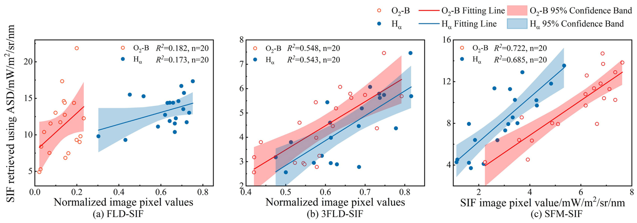
As shown in Figure 3, the SIF calculated by the FLD inversion method in the H_α band on the UAV platform (hereafter referred to as “H_α-FLD-SIF”) and the SIF obtained by the FLD inversion method in the O₂-B band (hereafter referred to as “O₂-B-FLD-SIF”) exhibited low fitting accuracy compared to the SIF calculated by ground ASD, with R² values of 0.173 and 0.182, respectively. The fitting accuracy for the SIF in the H_α band (hereafter referred to as “H_α-3FLD-SIF”) and the O₂-B band (hereafter referred to as “O₂-B-3FLD-SIF”) calculated by the 3FLD method using ground data showed some improvement, with R² values of 0.544 and 0.548, respectively. In the H_α band (hereafter referred to as “H_α-SFM-SIF”) and the O₂-B band (hereafter referred to as “O₂-B-SFM-SIF”), the highest fitting accuracy R² for SIF and ground calculation results obtained by SFM reached 0.685 and 0.723, respectively. In summary, the fitting accuracy of ground and UAV SIF data retrieved by the FLD method is the lowest, whereas that of the SFM is the highest. However, the difference between the SIF values retrieved from the ground and those retrieved by UAV is approximately doubled.

3.2. Correlation Analysis of Rs Rate and Image Band

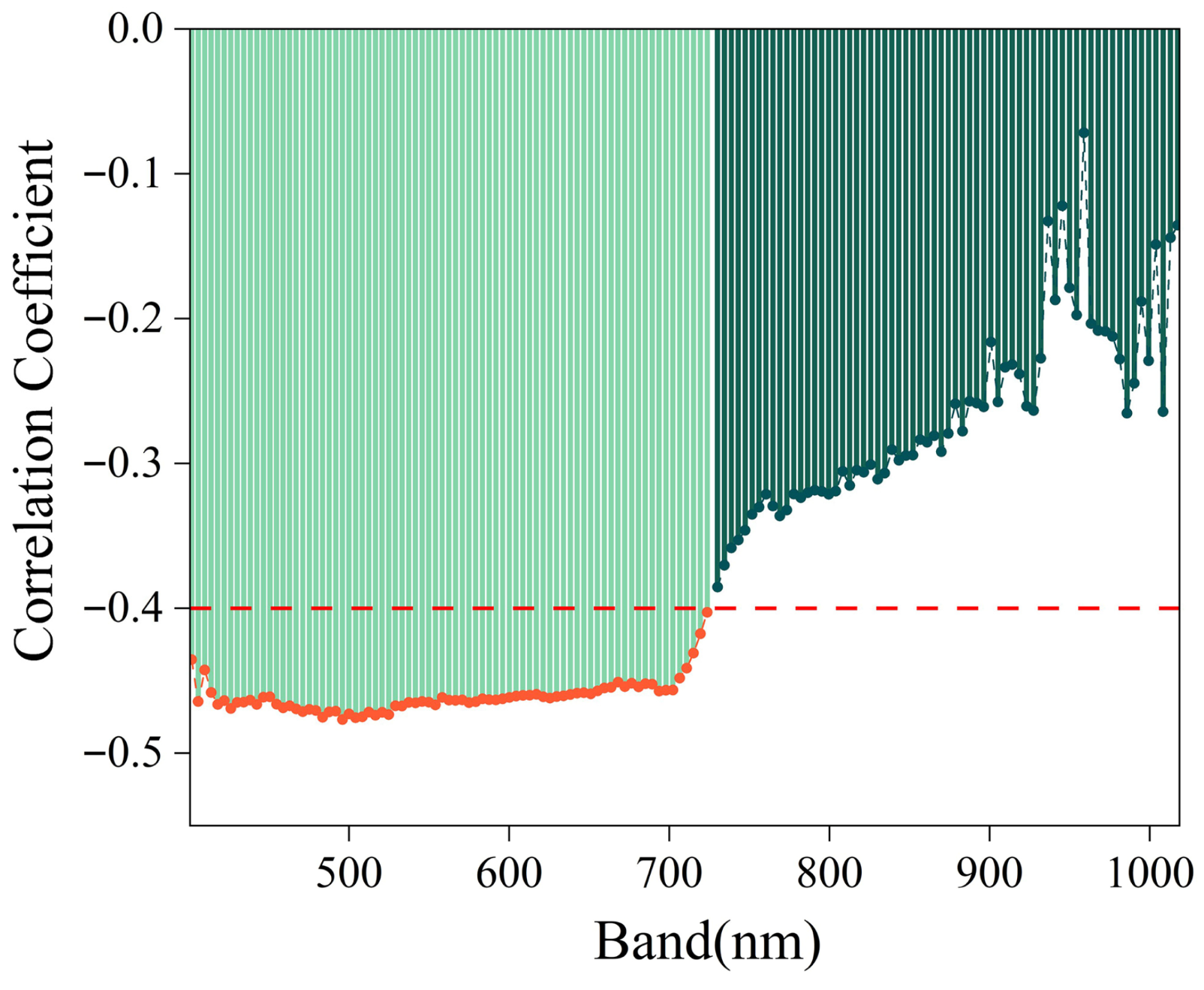
As illustrated in Figure 4, the Rs rate in the study area shows a negative correlation with the reflectance of each UAV band, and this correlation decreases sharply from around 720 nm, with a band exhibiting a “continuous aggregation” distribution through a 0.01 significance test (|correlation coefficient| > 0.4). It is noteworthy that within the 400–700 nm visible light range, the correlation coefficients exhibit remarkable consistency and stability. This “flat” distribution of correlations does not stem from sensor noise—as the UAV data have undergone rigorous radiometric calibration to compensate for spectral sensitivity variations—but rather reflects the high redundancy and strong similarity between adjacent bands in hyperspectral data [37]. Furthermore, it indicates a consistent response of surface reflectance to biophysical changes influencing Rs across the visible spectrum. However, the results from the coefficient correlation screening indicate similar values across many feature bands. This study employs differences in color light as the basis for secondary screening to minimize the number of feature bands. Within the spectral range of the selected feature bands, four color lights (purple, indigo, green, and red) are selected alongside the correlation coefficient values and the index selection scheme of current mainstream multi-spectral cameras [38]. Furthermore, four characteristic bands corresponding to the wavelength range of each light color are chosen to calculate the average value, which is used as the final band for modeling [39]. A total of four feature bands (

Table 3. Feature band screening results table.

Wavelength Range (nm)	Color Description	Correlation Coefficient (r)
435, 439, 443, 447	purple	−0.46
496, 500, 504, 509	indigo	−0.47
563, 567, 571, 576	green	−0.46
626, 630, 634, 639	red	−0.46

) were obtained using this method for the subsequent construction of the remote sensing model.

3.3. Selection of Vegetation Characterization Factors

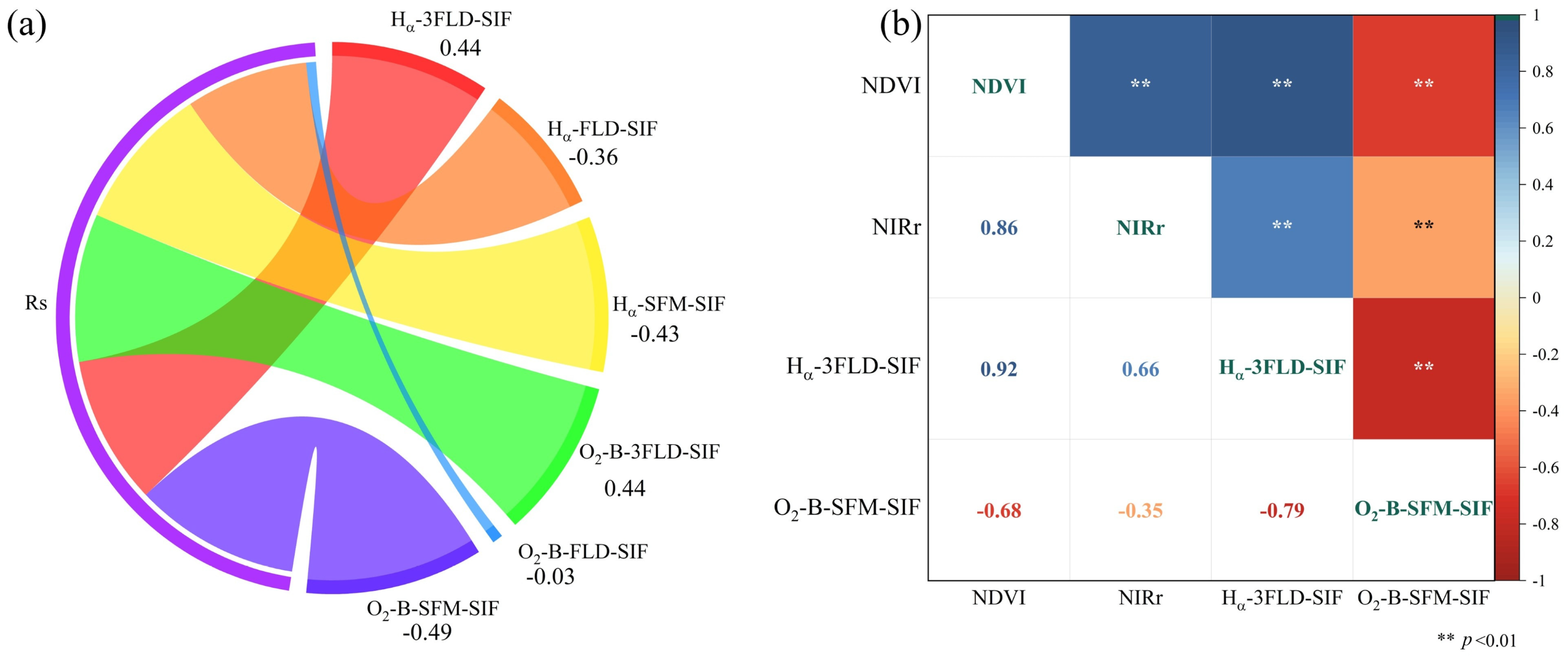
To compare and analyze the effects of various vegetation representation factors on remote sensing inversion modeling of Rs under vegetation cover in desert regions, this study first utilized the Pearson correlation coefficient method to compute the correlation between six types of SIF data and the measured Rs rate. As shown in Figure 5a, there was a significant positive correlation between H_α-3FLD-SIF and the Rs rate (p < 0.01), with a correlation coefficient of 0.44. The correlation between H_α-FLD-SIF and the Rs rate was low, resulting in a correlation coefficient of −0.36. A significant negative correlation existed between H_α-SFM-SIF and the Rs rate, with a correlation coefficient of −0.43. O₂-B-3FLD-SIF was positively correlated with the Rs rate, having a correlation coefficient of 0.44. No correlation was observed between O₂-B-FLD-SIF and the Rs rate, as the correlation coefficient was merely −0.03. The correlation between O₂-B-SFM-SIF and the Rs rate was the highest among all SIF data, reaching −0.49. The correlation between SIF retrieval and Rs rate through 3FLD and SFM is generally high. Considering the three factors of the inversion window, the inversion method, and correlation, H_α-3FLD-SIF and O₂-B-SFM-SIF are ultimately chosen as the representative SIF indicators for this study.

The principles and calculation methods for different vegetation factors differ significantly in the modeling process, and the vegetation information remains incomplete. Various vegetation factors were combined as modeling components to illustrate the growth conditions of vegetation better. A stronger correlation between the two vegetation factors indicates greater homogeneity; conversely, a weaker correlation highlights more significant differences between the two factors, accentuating the contrasting vegetation characteristics expressed [40]. Therefore, cross-correlation among different vegetation factors assesses whether their combination is necessary. Cross-correlation analysis was performed for NDVI, NIRv, H_α-3FLD-SIF, and O₂-B-SFM-SIF. Figure 5b indicates that the other indices display strong cross-correlation, except for the weak correlation between O₂-B-SFM-SIF and NIRv. Based on the results of the correlation analysis, the five characterized factor schemes of NDVI, NIRv, H_α-3FLD-SIF, O₂-B-SFM-SIF, and NIRv+O₂-B-SFM-SIF were ultimately established.

3.4. Influence of Different Combinations of Independent Variables on Modeling Accuracy

According to previous research results [41,42], this study utilized characteristic band, ST, SI, and TVDI as the “fixed part” of independent variables in modeling. It examined the differences in modeling performance among the five factors represented in Section 3.3 based on these variables. A comparative analysis illustrated the feasibility of using SIF for Rs inversion and the differences in inversion accuracy between SIF and traditional vegetation indices.

3.4.1. Make the “Fixed Part” Construct the Rs Model

First, the Rs inversion model was constructed using only the “fixed part,” without accounting for the influence of vegetation factors. As shown in

Table 4. Modeling results without using vegetation factors.

Model	Training Set		Test Set
	RMSE (μmol·m−2·s−1)	R2	RMSE (μmol·m−2·s−1)	R2
RF	0.09	0.69	0.09	0.50
PLSR	0.14	0.30	0.09	0.31
BP	0.10	0.40	0.15	0.45
SVM	0.12	0.36	0.11	0.36

, the absence of vegetation factors results in a generally low R² value for the model produced by the four machine learning methods, with the Random Forest (RF) method achieving the best performance (R² = 0.5, RMSE = 0.09 μmol·m⁻²·s⁻¹).

3.4.2. Feasibility Analysis and Modeling Accuracy Comparison of SIF Inversion of Rs

According to the five planting factors scheme detailed in Section 3.3, various vegetation factors were transformed based on the “fixed part.” A feasibility analysis of the SIF inversion of Rs and the modeling performance of different vegetation factors were compared and analyzed. Based on Table 4 and

Table 5. Modeling results of different vegetation representation factors.

Vegetation Factor	Model	Training Set		Test Set		Changing Situation (%) (Compared with Without Adding Vegetation Factors)
		RMSE (μmol·m−2·s−1)	R2	RMSE (μmol·m−2·s−1)	R2	RMSE (μmol·m−2·s−1)	R2
NDVI	RF	0.093	0.706	0.088	0.566	−2.2	13
	PLSR	0.130	0.308	0.125	0.308	38.9	−0.6
	BP	0.106	0.495	0.120	0.452	−20	0.4
	SVM	0.123	0.351	0.110	0.366	0	1.7
NIRv	RF	0.087	0.712	0.117	0.581	30	16.2
	PLSR	0.137	0.310	0.107	0.300	18.9	−3.2
	BP	0.120	0.397	0.136	0.409	−0.93	−9.1
	SVM	0.113	0.733	0.133	0.470	20.9	30.6
Hα-3FLD	RF	0.088	0.683	0.122	0.560	35.6	12
	PLSR	0.105	0.303	0.168	0.302	86.7	−2.6
	BP	0.112	0.366	0.133	0.373	−11.3	−17.1
	SVM	0.115	0.431	0.108	0.407	−1.8	13.1
O2-B-SFM-SIF	RF	0.083	0.694	0.127	0.634	41.1	26.8
	PLSR	0.112	0.314	0.148	0.357	64.4	15.2
	BP	0.117	0.437	0.109	0.445	−27.3	−1.1
	SVM	0.117	0.808	0.101	0.361	−8.1	0.3
NIRv+ O2-B-SFM-SIF	RF	0.090	0.681	0.103	0.579	14.4	15.8
	PLSR	0.122	0.312	0.126	0.313	40	1
	BP	0.111	0.492	0.121	0.458	−19.3	1.8
	SVM	0.127	0.784	0.114	0.415	3.6	15.3

, RF showed the best inversion effect among the four machine learning methods. After incorporating vegetation factors, the accuracy of the Rs inversion models constructed by RF improved to varying degrees, indicating that vegetation is a crucial influencing factor of Rs that cannot be overlooked, even in desert ecosystems with limited vegetation. As shown in Table 5, when NDVI was included in the modeling, the R² of the model increased by 13%. The RMSE decreased by 2.2% (R² = 0.566, RMSE = 0.088 μmol·m⁻²·s⁻¹), suggesting that NDVI was ineffective for Rs inversion in sparse vegetation areas; however, when NIRv was utilized for modeling, the RF model R² increased by 16.2%, while RMSE rose by 30% (R² = 0.581, RMSE = 0.117 μmol·m⁻²·s⁻¹). Compared to NDVI, the accuracy of the NIRv model improved to some extent. The results indicate that the vegetation index corrected by radiance was more suitable for Rs retrieval than NDVI. When H_α-3FLD-SIF was used for modeling, the model R² increased by 12%, similar to that of NDVI, but RMSE rose by 35.6% (R² = 0.56, RMSE = 0.122 μmol·m⁻²·s⁻¹). The RF inversion model based on O₂-B-SFM-SIF achieved the highest accuracy (R² = 0.63, RMSE = 0.127 μmol·m⁻²·s⁻¹), with the test set R² being 26.8% higher than that without vegetation factors and 13.8% and 10.6% higher than those with NDVI and NIRv, respectively. The test set RMSE increased by 41.1%. When NIRv + O₂-B-SFM-SIF was employed for modeling, R² and RMSE increased by 15.8% and 14.4% (R² = 0.579, RMSE = 0.103 μmol·m⁻²·s⁻¹) compared to the non-vegetation model. Compared to the previously mentioned vegetation factor models, except for O₂-B-SFM-SIF, the accuracy improvement was insignificant, and the modeling accuracy resembled that of NIRv. The results indicated that combining SIF and the vegetation index did not effectively reflect the photosynthetic activity of vegetation and may reduce the modeling accuracy of Rs.

In summary, SIF can be used for remote sensing of Rs inversions, and the modeling accuracy significantly surpasses that of the traditional optical vegetation index NDVI and NIRv. Even in desert regions with sparse vegetation, Rs inversion accuracy can still be achieved using SIF.

3.5. Spatial Inversion of Soil Respiration and Evaluation of Accuracy

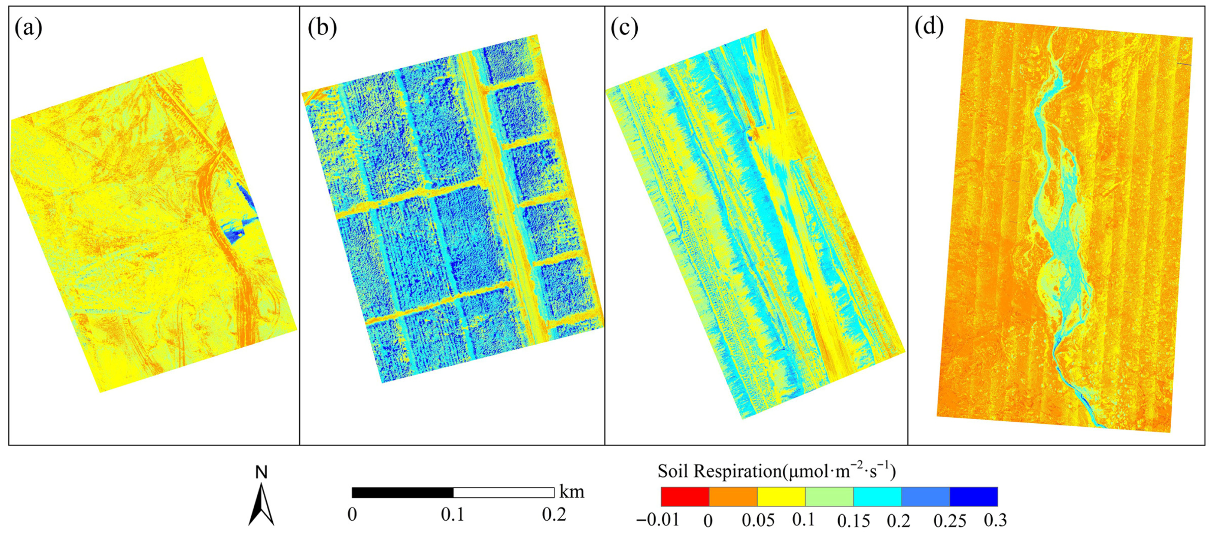
In Section 3.4, by comparing various vegetation factor modeling schemes, it was found that the accuracy of the Rs inversion model constructed using O₂-B-SFM-SIF as a vegetation characterization factor was superior to that of other optical vegetation indices. Based on the inversion model, the feature band images of UAV, ST, TVDI, and SIF were used to create the Rs spatial distribution map in the study area (Figure 6).

The Rs rates of different plots in the study area are as follows: Tamarisk forest (0.159 ± 0.1 μmol·m⁻²·s⁻¹), red sand spring (0.158 ± 0.122 μmol·m⁻²·s⁻¹), plantation (0.22 ± 0.14 μmol·m⁻²·s⁻¹), and dump (0.172 ± 0.12 μmol·m⁻²·s⁻¹). The predicted results closely align with the measured values. The findings indicate that the Rs rate went from high to low, from plantation > dump > Hongsha spring ≈ Tamarisk forest.

As shown in Figure 6a, Rs in the Tamarisk forest area is generally low and is influenced by the presence of plants. The Rs rate in the vegetated area is significantly higher than in the bare land. In the plantation reclamation area (Figure 6b), where land reclamation has been implemented and vegetation is relatively lush, the spatial distribution characteristics of Rs align with those of the vegetation. The vegetation cover in this area leads to heightened Rs activity. In the reclamation area of the dump site (Figure 6c), microbial restoration technology was employed to rehabilitate the region, resulting in improved Rs levels wherever vegetation has grown. Additionally, the slope surface between different platforms of the dump site also exhibited an increase in Rs. In the Hongsha spring area (Figure 6d), it is evident that the Rs in regions fed by central spring water are significantly higher than in non-flowing areas, and the Rs in areas with lush vegetation flanking the water flow are correspondingly elevated.

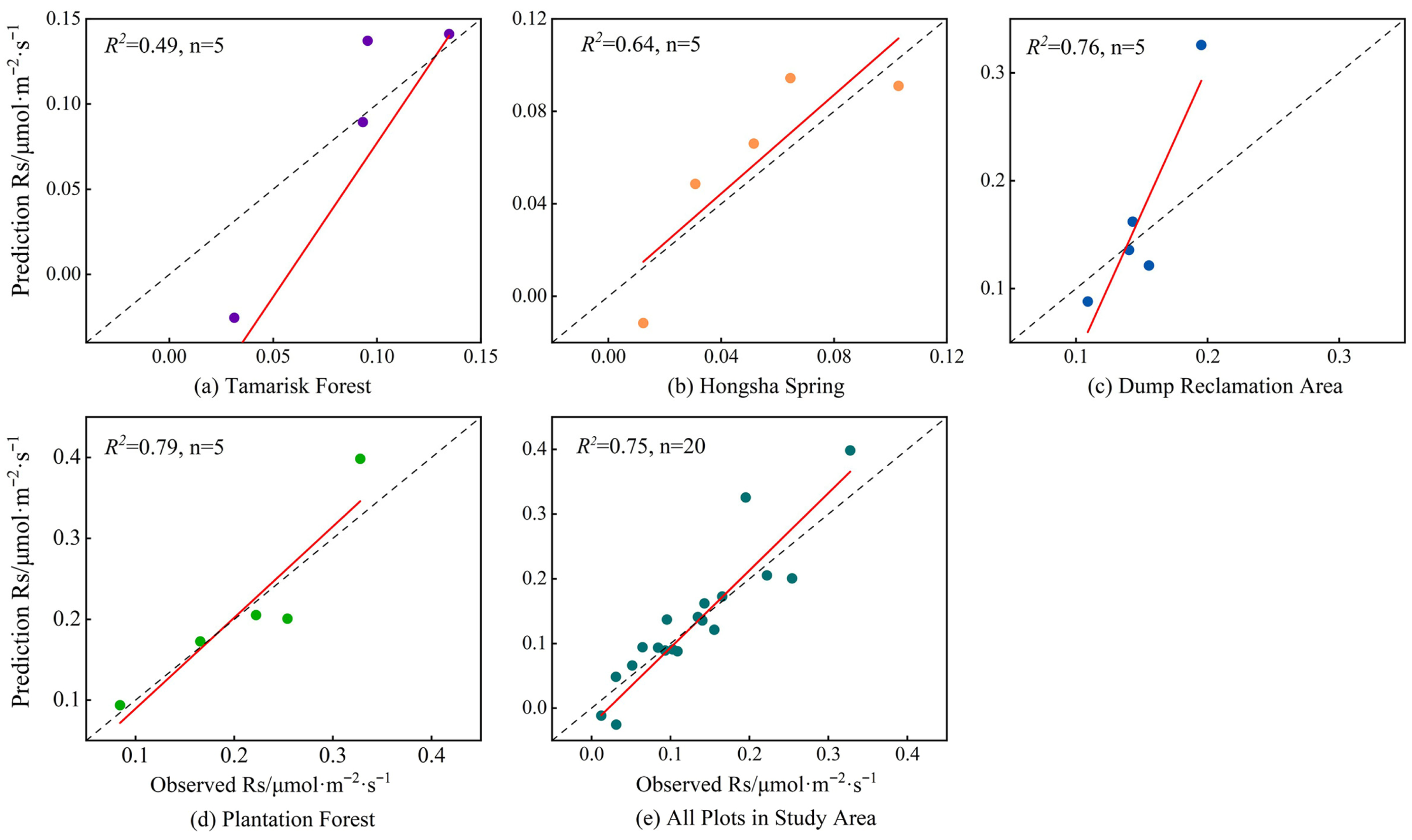
To verify the prediction accuracy of the Rs inversion model, five measured points (out of twenty in the study area) were reserved for each plot and not included in the modeling. As shown in Figure 7, the fitting R² of the Rs rate predicted by the Tamarix forest (Figure 7a) and Hongsha spring (Figure 7b), along with the measured Rs, was 0.49 (p > 0.05) and 0.64 (p > 0.05), respectively. Neither value achieved the 95% significance threshold, suggesting that the inversion accuracy of the Rs inversion models in these two regions was insufficient. However, the fitting R² between the predicted Rs rate and the measured Rs rate at the dump site (Figure 7c) and plantation forest (Figure 7d) was 0.76 (p < 0.05) and 0.79 (p < 0.05), respectively, and both passed the 95% significance test. This inversion accuracy was considerably higher than that of the Tamarix forest and Hongsha spring, primarily due to the significantly higher vegetation coverage in these two reclamation areas compared to the former. The vegetation was lusher. Considering all sample sites (Figure 7e), the model’s inversion accuracy was notable, with a fitting R² of 0.75 (p < 0.05) between the predicted Rs rate and the measured Rs rate, which also passed the 95% significance test.

In summary, using the measured Rs rate as the dependent variable and the characteristic bands, ST, SI, TVDI, and O₂-B-SFM-SIF as the independent variables for modeling, the Rs inversion model constructed using RF can accurately invert the spatial distribution of Rs in areas with dense vegetation. The inversion accuracy of the model decreases in regions with sparse vegetation. However, the model’s inversion values remain close to the measured values in areas with vegetation cover. The research findings suggest that SIF is more effective than traditional optical vegetation indices in Rs remote sensing inversion. The information related to vegetation photosynthetic activity provided by SIF is richer than that from vegetation indices. SIF’s unique “mechanical” characteristics offer advantages in quantitative remote sensing. Consequently, the Rs inversion model based on SIF can more accurately predict the spatial distribution of Rs. These results provide new ideas and methods for studying the carbon cycle in deserts and other ecosystems.

4. Discussion

4.1. Estimating Rs Potential Using SIF

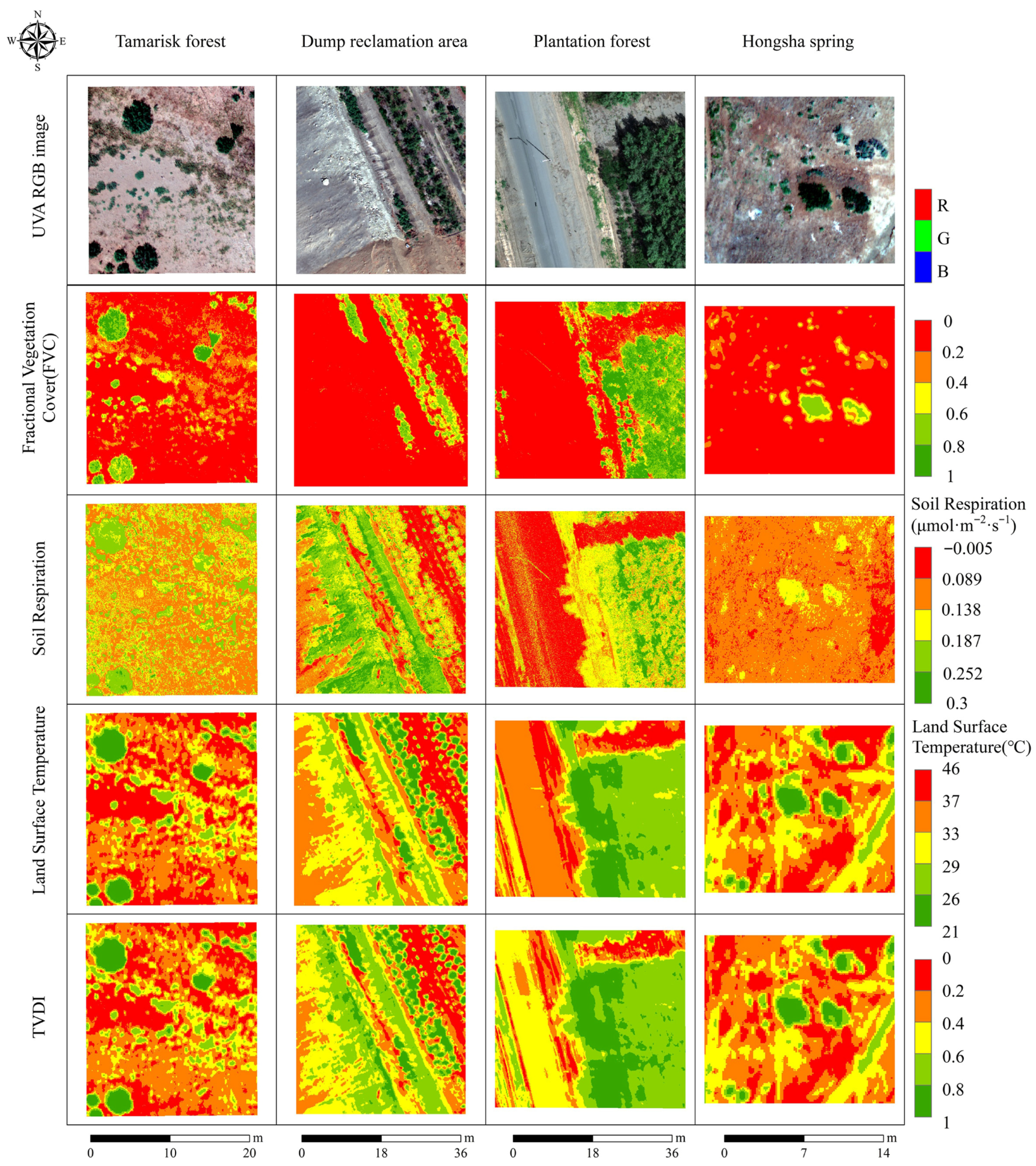
SIF is directly related to photosynthesis in vegetation. It is often utilized as a mechanistic representation factor for vegetation in contexts such as drought stress, pest monitoring, and the ecosystem carbon cycle. Research on the carbon cycle primarily examines the relationship between SIF and GPP and has informed studies on changes in atmospheric CO₂ levels [43]. However, research on remote sensing inversion of Rs through SIF is quite limited due to limitations regarding the accuracy of remote sensing signals for vegetation fluorescence, physiological processes associated with plant growth, and local soil conditions. Most existing studies have relied on traditional vegetation indices as representation factors. For instance, Chen et al. [44] used LAI to explore global annual Rs variations, while Jagermeyr et al. [45] employed EVI to estimate ecosystem respiration on a continental scale. To date, there are no reports of using SIF to estimate Rs, primarily due to: (1) the limited accuracy of SIF remote sensing solutions, challenges related to the structure of vegetation canopies, and the reabsorption of elements within leaves and the atmosphere [27]; (2) Rs generated from both autotrophic respiration of plant roots and heterotrophic respiration by soil microorganisms, which is influenced by temperature, humidity, soil microorganisms, plant growth conditions, and other factors [25]. The presence of multiple parameters in remote sensing inversion also implies that the sensitivity of these parameters varies across regions, leading to potential inversion errors [46,47]. (3) The diffusion process of Rs within the soil medium is still not fully understood [48]. A better understanding of Rs emissions in vegetated areas can be developed by linking the soil’s respiration emission rate to that measured through ground observations, laying solid scientific groundwork for the ecosystem’s carbon budget, and predicting future shifts in carbon sources and sinks. In this study, no strict physiological process models were applied to the modeling. Instead, ST, SM, SI, and SIF, along with characteristic bands, were utilized as independent variables for modeling, leading to the development of a statistical model for Rs remote sensing inversion using machine learning. While this model produced a more accurate spatial distribution of Rs, it lacked a mechanistic explanation. As shown in Figure 7, the inversion accuracy for Rs rates is higher in reclamation areas of waste dumps and plantations but less accurate in Tamarisk forests and the Hongsha spring. The vegetation species in the plantation and dump areas included elm, sea buckthorn, and Tamarisk, respectively, with a relatively dense canopy, resulting in better SIF quality from inversion. In contrast, Tamarisk forests and Hongsha spring predominantly feature sparse desert vegetation, leading to poorer SIF accuracy retrieval. Despite these discrepancies, the accuracy of the Rs inversion model based on SIF exceeds that of traditional optical vegetation indices. This suggests that using SIF to monitor Rs is both feasible and precise. Future studies should incorporate mechanistic models to enhance generalization performance and application across different scenarios, contributing innovative insights for the global quantitative survey of Rs. Fractional Vegetation Cover (FVC) is calculated within the study area, utilizing various local image maps (Figure 8) to analyze the spatial distribution characteristics of Rs, vegetation, and other factors. As illustrated in Figure 8, the spatial distribution of FVC and Rs correspond to each other, with Rs being more potent in areas exhibiting significant vegetation growth. However, notable phenomena arise, such as in the Tamarisk forest and Hongshaquan area, where the FVC is slightly smaller than the retrieved Rs. Significant Rs is also observed in areas lacking vegetation cover in both dump and plantation zones. Insights into this phenomenon can be gleaned from LST and TVDI images. In the specific humidity region of bare soil (with a TVDI around 0.4), the bare soil temperature in the dump area reaches about 30 °C, which is similarly observed in artificial forests. This indicates that soil temperature and humidity substantially influence Rs, consistent with existing research findings [49]. In the Tamarisk forest and Hongsha spring, the growth of desert vegetation improves soil conditions to some extent, reduces surface temperature, maintains soil moisture, and promotes increases in Rs.

4.2. Preprocessing and Feature Extraction of Hyperspectral Data

The primary feature of hyperspectral data is its ultra-high spectral resolution. Although it contains rich information, there is also significant information redundancy. Therefore, it is essential to emphasize the differences between bands through data preprocessing to achieve better results in subsequent feature extraction [50]. This study examined the root and logarithmic reciprocal transformations of hyperspectral reflectance images. It was found that the correlation between the bands and the measured Rs data did not improve significantly after the mathematical transformation. However, the correlation among the band data post-transformation still displayed a clustered distribution, with the absolute value of the correlation remaining relatively stable (around 0.5). Given this, the hyperspectral data used in this study is not mathematically transformed; the band reflectance is used directly for modeling. Some common spectral pretreatment methods, such as Standard Normal Variate Transformation (SNV) and Multiple Scattering Correction (MSC), are widely employed for treating individual sample spectra. However, they are not suitable for processing image-dimensional spectral data. To mitigate the effects of scattering on the spectrum, these two methods must compute the mean value of multiple spectral curves of the same ground object before performing the corresponding mathematical calculations. However, since the ground objects corresponding to each pixel of the hyperspectral image are not identical, these preprocessing methods cannot be used to process the hyperspectral image.

Since the correlation between adjacent bands of hyperspectral data is very high, correlation coefficient screening is typically performed twice to retain sufficient information and reduce redundancy. The Successive Projections Algorithm (SPA) [51] or Competitive Adaptive Reweighted Sampling (CARS) [52] algorithms may be utilized to refine the screening results. However, the bands that were highly correlated with the measured Rs rate clustered and showed a distribution according to the correlation analysis in this study (Figure 2), resulting in a situation where all bands were characteristic bands using the secondary screening method, which failed to achieve dimensionality reduction. Therefore, this study refers to the visible spectrum and considers the differences among bands of light colors. Based on these color differences, four characteristic bands are ultimately identified as part of the independent variables for modeling.

4.3. Problems with SIF Search

Currently, SIF near-surface inversion methods are developed based on the Fraunhofer dark line method proposed by Plascyk and Gabriel [31]. Through ongoing exploration and optimization, researchers have proposed various improved algorithms, such as 3FLD, iFLD, SFM, etc. When addressing SIF, researchers employed dark bands near 687 nm and 760.6 nm in the solar spectrum, known as the O₂-B band and O₂-A band [43]. Among these, the O₂-A band is most frequently utilized due to its more significant element absorption effect, deeper absorption valley, and reduced SIF signal reabsorption by the leaf [53]. In this study, limitations of the hyperspectral image acquisition equipment in retrieving SIF present several challenges: (1) The amplitude error of homogeneous pixels in the same field image for the O₂-A band is approximately ±15%, resulting in irretrievable band noise in the retrieved SIF, thus making the O₂-A band unsuitable for SIF inversion; (2) According to research by Meroni and Colombo [54], retrieving SIF with SFM requires a high spectral resolution (≤0.1 nm) in the inversion window to provide sufficient irradiance and radiance for the inversion of the undetermined coefficient [53]. However, the spectral resolution of the hyperspectral image data used in this study is 4 nm, which does not meet SFM’s requirements, and the absorption valley cannot be adequately reconstructed through interpolation, leading to poor inversion performance. Consequently, the simplified SFM proposed by Meroni and Colombo [54] was ultimately chosen for retrieving SIF values in the two windows. However, this simplified method assumes that the SIF and actual reflectance in the inversion window are constant, which is inconsistent with the exact conditions. These two factors contribute to errors in the SIF signals retrieved by UAVs. In subsequent research, it is necessary to improve spectral acquisition equipment to enhance spectral resolution and the accuracy of SIF retrieval, thereby increasing the remote sensing inversion accuracy of Rs.

5. Conclusions

Using four machine learning methods, this study utilized UAV hyperspectral data and ground Rs data to assess the quantitative inversion performance of Rs across three factors, NDVI, NIRv, and SIF. The results indicate that acquiring characteristic bands, correlation with spectral index, and SIF through UAV enables Rs estimation. Employing SIF in modeling enhances accuracy by 41.1%. Among the methods, the Random Forest approach based on O₂-B-SFM-SIF achieved the highest accuracy (R² = 0.63, RMSE = 0.127 μmol·m⁻²·s⁻¹) for remote sensing estimation of Rs, demonstrating that SIF is a viable option for estimating Rs in desertification mining areas. Additionally, this study found that SIF allows for estimating ground Rs and surpasses traditional optical vegetation indices (NDVI, NIRv) in accuracy during Rs modeling. When using SIF as an independent variable, the model’s accuracy improved by 13.8% compared to NDVI and 10.6% compared to NIRv. The findings of this study contribute to understanding SIF’s potential for remote sensing inversion of Rs, offer a fresh perspective for improving the accuracy of carbon cycle estimations in sandy mining areas, and serve as a reference for large-scale remote sensing estimations of Rs.

References

1. Wang, J.Y.; Wei, J.; Wen, X.F. Advances in theory, hypothesis and application of soil CO2 flux gradient observation techniques and methods. J. Plant Ecol. 2022, 46, 1523–1536. [Google Scholar] [CrossRef]
2. Xiao, W.; Zhang, W.; Ye, Y.; Lv, X.; Yang, W. Is underground coal mining causing land degradation and significantly damaging eco-systems in semi-arid areas? A study from an Ecological Capital perspective. Land Degrad. Dev. 2020, 31, 1969–1989. [Google Scholar] [CrossRef]
3. Ahirwal, J.; Maiti, S.K.; Singh, A.K. Changes in ecosystem carbon pool and soil CO2 flux following post-mine reclamation in dry tropical environment, India. Sci. Total Environ. 2017, 583, 153–162. [Google Scholar] [CrossRef]
4. Huang, Y.; Tian, F.; Wang, Y.; Wang, M.; Hu, Z. Effect of coal mining on vegetation disturbance and associated carbon loss. Environ. Earth Sci. 2015, 73, 2329–2342. [Google Scholar] [CrossRef]
5. Subke, J.A.; Inglima, I.; Cotrufo, M.F. Trends and methodological impacts in soil CO2 efflux partitioning: A metanalytical review. Glob. Change Biol. 2006, 12, 921–943. [Google Scholar] [CrossRef]
6. Cui, H.J.; Liu, J.; Du, Z.Q.; Yan, J.; Jiao, X. Hyperspectral characteristics of sorghum under biochar and mulch and their ccrelationship with soil respiration. Res. Soil Water Conserv. 2020, 27, 15–22. [Google Scholar]
7. Huang, N.; Wang, L.; Song, X.P.; Black, T.A.; Jassal, R.S.; Myneni, R.B.; Wu, C.; Wang, L.; Song, W.; Ji, D.; et al. Spatial and temporal variations in global soil respiration and their relationships with climate and land cover. Sci. Adv. 2020, 6, eabb8508. [Google Scholar] [CrossRef]
8. Azevedo, O.; Parker, T.C.; Siewert, M.B.; Subke, J.-A. Predicting soil respiration from plant productivity (NDVI) in a sub-Arctic tundra ecosystem. Remote Sens. 2021, 13, 2571. [Google Scholar] [CrossRef]
9. Weiland, L.; Rogers, C.A.; Sothe, C.; Arain, M.A.; Gonsamo, A. Satellite-based land surface temperature and soil moisture observations accurately predict soil respiration in temperate deciduous and coniferous forests. Agric. For. Meteorol. 2023, 340, 109618. [Google Scholar] [CrossRef]
10. Lee, M.S.; Nakane, K.; Nakatsubo, T.; Koizumi, H. Seasonal changes in the contribution of root respiration to total soil respiration in a cool-temperate deciduous forest. Plant Soil 2003, 255, 311–318. [Google Scholar] [CrossRef]
11. Yang, Y.L.; Chen, Y.P.; Yao, C.P.; Zheng, Y. Contribution of root respiration of different psammophytes to soil respiration. J. Lanzhou Jiaotong Univ. 2022, 41, 115–122. (In Chinese) [Google Scholar]
12. Liu, P.; Jia, X.; Yang, Q.; Zha, T.; Wang, B.; Ma, J. Soil respiration characteristics of Artemisia Orcharis shrub ecosystem in Mu Us Sandy Land. Sci. Silvae Sin. 2018, 54, 10–17. [Google Scholar]
13. Zhou, X.; Zhang, Y. Seasonal pattern of soil respiration and gradual changing effects of nitrogen addition in a soil of the Gurbantunggut Desert, northwestern China. Atmos. Environ. 2014, 85, 187–194. [Google Scholar] [CrossRef]
14. Mukhopadhyay, S.; Maiti, S.K. Soil CO2 flux in grassland, afforested land and reclaimed coalmine overburden dumps: A case study. Land Degrad. Dev. 2014, 25, 216–227. [Google Scholar] [CrossRef]
15. Ren, Z.S.; Qi, R.P.; Wang, T.T.; Xie, Q.; Zheng, J.Y.; Zhang, X.C. Effect of weathered coal on soil respiration of newly constructed soil in the dump of Jinshaan-Menghui Mining area. Trans. Chin. Soc. Agric. Eng. 2015, 31, 230–237. [Google Scholar]
16. Fang, P.; Yao, X.Y.; Dong, R.X.; Bu, W.C.; Li, H.D.; Yang, W.L.; Liu, Y.; Yue, H. Research progress on characteristics and driving mechanism of soil CO2 emission in mining areas. J. Min. Sci. Technol. 2026, 11, 63–74. [Google Scholar]
17. Liu, Y.; Lin, J.Q.; Yue, H.; Bi, Y.L.; Peng, S.P. Soil respiration and its influencing factors of different land use types in desertification mining area. J. Coal Sci. Eng. 2023, 48, 2893–2905. [Google Scholar]
18. Damm, A.; Elbers, J.A.N.; Erler, A.; Gioli, B.; Hamdi, K.; Hutjes, R.; Kosvancova, M.; Meroni, M.; Miglietta, F.; Moersch, A.; et al. Remote sensing of sun-induced fluorescence to improve modeling of diurnal courses of gross primary production (GPP). Glob. Change Biol. 2010, 16, 171–186. [Google Scholar] [CrossRef]
19. Frankenberg, C.; Fisher, J.B.; Worden, J.; Badgley, G.; Saatchi, S.S.; Lee, J.-E.; Toon, G.C.; Butz, A.; Jung, M.; Kuze, A.; et al. New global observations of the terrestrial carbon cycle from GOSAT: Patterns of plant fluorescence with gross primary productivity. Geophys. Res. Lett. 2011, 38, L17706. [Google Scholar] [CrossRef]
20. Guanter, L.; Zhang, Y.; Jung, M.; Joiner, J.; Voigt, M.; Berry, J.A.; Frankenberg, C.; Huete, A.R.; Zarco-Tejada, P.; Lee, J.-E.; et al. Global and time-resolved monitoring of crop photosynthesis with chlorophyll fluorescence. Proc. Natl. Acad. Sci. USA 2014, 111, E1327–E1333. [Google Scholar] [CrossRef]
21. Lee, J.E.; Frankenberg, C.; Van der Tol, C.; Berry, J.A.; Guanter, L.; Boyce, C.K.; Fisher, J.B.; Morrow, E.; Worden, J.R.; Asefi, S.; et al. Forest productivity and water stress in Amazonia: Observations from GOSAT chlorophyll fluorescence. Proc. R. Soc. B Biol. Sci. 2013, 280, 20130171. [Google Scholar] [CrossRef]
22. Zhang, Y.; Guanter, L.; Berry, J.A.; Joiner, J.; van der Tol, C.; Huete, A.; Gitelson, A.; Voigt, M.; Köhler, P. Estimation of vegetation photosynthetic capacity from space-based measurements of chlorophyll fluorescence for terrestrial biosphere models. Glob. Change Biol. 2014, 20, 3727–3742. [Google Scholar] [CrossRef]
23. Wang, S.; Huang, C.; Zhang, L.; Lin, Y.; Cen, Y.; Wu, T. Monitoring and assessing the 2012 drought in the great plains: Analyzing satellite-retrieved solar-induced chlorophyll fluorescence, drought indices, and gross primary production. Remote Sens. 2016, 8, 61. [Google Scholar] [CrossRef]
24. Yue, H.; Zhu, R.; Liu, Y.; Wei, J.L.; Bi, Y.L.; Jiang, K.S. Construction of soil moisture monitoring model in desertification open-pit mine: A case study of Hongshaquan Mining area. Coal Sci. Technol. 2022, 50, 300–311. [Google Scholar]
25. Wu, K.N.; Zhao, R. Classification of soil texture and its application in China. Acta Pedol. Sin. 2019, 56, 227–241. [Google Scholar]
26. Liu, Y.; Lin, J.; Yue, H. Soil respiration estimation in desertified mining areas based on UAV remote sensing and machine learning. Earth Sci. Inform. 2023, 16, 3433–3448. [Google Scholar] [CrossRef]
27. Wu, D.Y.; Wang, X.J.; Lei, H.M. Construction of soil autotrophic and heterotrophic respiration models in winter wheat-summer maize farmland ecosystem in North China Plain. Ecol. Sin. 2024, 6, 2364–2378. [Google Scholar]
28. He, L.; Chen, J.M.; Liu, J.; Mo, G.; Joiner, J. Angular normalization of GOME-2 Sun-induced chlorophyll fluorescence observation as a better proxy of vegetation productivity. Geophys. Res. Lett. 2017, 44, 5691–5699. [Google Scholar] [CrossRef]
29. Gong, E.J. Spatial and Temporal Dynamics and Influencing Factors of Terrestrial Ecosystem GPP in China in Recent 20 Years. Ph.D. Thesis, North China University of Water Resources and Electric Power, Zhengzhou, China, 2023. (In Chinese) [Google Scholar]
30. Maier, S.W.; Günther, K.P.; Stellmes, M. Sun-induced fluorescence: A new tool for precision farming. Digit. Imaging Spectr. Tech. Appl. Precis. Agric. Crop Physiol. 2004, 66, 207–222. [Google Scholar]
31. Plascyk, J.A.; Gabriel, F.C. The Fraunhofer line discriminator MKII-an airborne instrument for precise and standardized ecological luminescence measurement. IEEE Trans. Instrum. Meas. 1975, 24, 306–313. [Google Scholar] [CrossRef]
32. Meroni, M.; Rossini, M.; Guanter, L.; Alonso, L.; Rascher, U.; Colombo, R.; Moreno, J. Remote sensing of solar-induced chlorophyll fluorescence: Review of methods and applications. Remote Sens. Environ. 2009, 113, 2037–2051. [Google Scholar] [CrossRef]
33. Zeng, Y.; Badgley, G.; Dechant, B.; Ryu, Y.; Chen, M.; Berry, J.A. A practical approach for estimating the escape ratio of near-infrared solar-induced chlorophyll fluorescence. Remote Sens. Environ. 2019, 232, 111209. [Google Scholar] [CrossRef]
34. Kriegler, F.J.; Malila, W.A.; Nalepka, R.F.; Richardson, W. Preprocessing transformations and their effects on multispectral recognition. In Proceedings of the Sixth International Symposium on Remote Sensing of Environment, Ann Arbor, MI, USA, 13–16 October 1969; pp. 97–131. [Google Scholar]
35. Allbed, A.; Kumar, L.; Aldakheel, Y.Y. Assessing soil salinity using soil salinity and vegetation indices derived from IKONOS high-spatial resolution imageries: Applications in a date palm dominated region. Geoderma 2014, 230, 1–8. [Google Scholar] [CrossRef]
36. Sandholt, I.; Rasmussen, K.; Andersen, J. A simple interpretation of the surface temperature/vegetation index space for assessment of surface moisture status. Remote Sens. Environ. 2002, 79, 213–224. [Google Scholar] [CrossRef]
37. Li, T.X.; Zhang, F.; Feng, J. Convolutional neural network combined with improved spectral processing method for potato disease detection. Spectrosc. Spectr. Anal. 2024, 44, 215–224. [Google Scholar]
38. Zhang, Z.H.; Gan, F.P.; Wang, J. Discussion on index setting of Spaceborne Multispectral camera based on Application requirements. Remote Sens. Nat. Resour. 2015, 27, 1–7. [Google Scholar]
39. Zhang, L.; Liu, L.Y.; Gao, J.W.; Jiao, Q.J.; Jia, J.H. Exploration of remote sensor band setting based on ant colony optimization algorithm. Remote Sens. Technol. Appl. 2016, 31, 488–496. [Google Scholar]
40. Luo, L.L. Remote Sensing Research on Maize Physiological and Biochemical Parameters Based on Ground and Low-Altitude UAVs. Ph.D. Thesis, Northwest A&F University, Yangling, China, 2022. (In Chinese) [Google Scholar]
41. Liu, S.H.; Fang, J.Y. Factors influencing soil respiration and effects of temperature on global scale. Acta Ecol. Sin. 1997, 5, 19–26. [Google Scholar]
42. Wang, X.Y.; Li, Y.L.; Zhao, X.Y.; Mao, W.; Cui, D.; Qu, H.; Lian, J.; Luo, Y.Q. Research progress on effects of different environmental factors on soil respiration in arid and semi-arid regions. Acta Ecol. Sin. 2012, 32, 4890–4901. [Google Scholar] [CrossRef]
43. Zhang, Z.Y.; Wang, S.H.; Qiu, B.; Song, L.; Zhang, Y.G. Remote sensing inversion of Sun induced chlorophyll fluorescence and its application in carbon cycle. J. Remote Sens. 2019, 23, 37–52. [Google Scholar]
44. Chen, S.; Zou, J.; Hu, Z.; Chen, H.; Lu, Y. Global annual soil respiration in relation to climate, soil properties and vegetation characteristics: Summary of available data. Agric. For. Meteorol. 2014, 198, 335–346. [Google Scholar] [CrossRef]
45. Jägermeyr, J.; Gerten, D.; Lucht, W.; Hostert, P.; Migliavacca, M.; Nemani, R. A high-resolution approach to estimating ecosystem respiration at continental scales using operational satellite data. Glob. Change Biol. 2014, 20, 1191–1210. [Google Scholar] [CrossRef] [PubMed]
46. Hibbard, K.A.; Law, B.E.; Reichstein, M.; Sulzman, J. An analysis of soil respiration across northern hemi-sphere temperate ecosystems. Biogeochemistry 2005, 73, 29–70. [Google Scholar] [CrossRef]
47. Chen, S.T.; Zou, J.W.; Hu, Z.H. Observation and simulation of soil respiration in terrestrial ecosystem. J. Ecol. Environ. 2017, 26, 1985–1996. [Google Scholar]
48. Wang, G.; Zhou, J. Multiobjective optimization of carbon emission reduction responsibility allocation in the open-pit mine production process against the background of peak carbon dioxide emissions. Sustainability 2022, 14, 9514. [Google Scholar] [CrossRef]
49. Wang, B.; Jiang, Y.; Guo, H.; Zhao, G.D.; Bai, X.L. Study on soil respiration and its three biological processes. Chin. J. Soil Sci. 2011, 42, 483–490. [Google Scholar]
50. Di, W.P.Y.; Bian, X.H.; Wang, Z.F.; Liu, W. Study on the selection of spectral pretreatment methods. Spectrosc. Spectr. Anal. 2019, 39, 2800–2806. [Google Scholar]
51. Deng, F.; Ding, Y.; Chen, Y.J.; Zhu, S.N.; Chen, F.F. Quantitative analysis of the content of nitrogen and sulfur in coal based on laser-induced breakdown spectroscopy: Effects of variable selection. Plasma Sci. Technol. 2020, 22, 074005. [Google Scholar] [CrossRef]
52. Zhao, X.H.; Feng, X.Q.; Nie, X.J.; Zhang, Y.; Guo, E.H. Estimation of soil phosphorus content in mining area based on CARS-CNN and hyperspectral remote sensing. Chin. J. Ecol. 2024, 43, 3553–3562. [Google Scholar]
53. Wu, L.; Zhang, Y.; Zhang, Z.; Zhang, X.; Wu, Y.; Chen, J.M. Deriving photosystem-level red chlorophyll fluorescence emission by combining leaf chlorophyll content and canopy far-red solar-induced fluorescence: Possibilities and challenges. Remote Sens. Environ. 2024, 304, 114043. [Google Scholar] [CrossRef]
54. Meroni, M.; Colombo, R. Leaf level detection of solar induced chlorophyll fluorescence by means of a subnanometer resolution spectroradiometer. Remote Sens. Environ. 2006, 103, 438–448. [Google Scholar] [CrossRef]
Figure 1. The study area includes the locations of the Hongshaquan mining area and the experimental plot. (ad) UAV RGB images of Tamarix forest, plantation forest, dump reclamation area, and Hongsha spring, respectively.
Remotesensing 18 01475 g001
Figure 2. Technical roadmap.
Remotesensing 18 01475 g002
Figure 3. UAV and ground ASD retrieve SIF accuracy maps using different SIF retrieval methods; (ac) the SIF results corresponding to different retrieval methods.
Remotesensing 18 01475 g003
Figure 4. Map of the correlation coefficient between drone band and Rs.
Remotesensing 18 01475 g004
Figure 5. (a) Different UAV SIF and Rs correlation diagram; (b) the four planting factors were characterized by mutual correlation heat maps.
Remotesensing 18 01475 g005
Figure 6. Spatial distribution of Rs; (ad) Tamarix forest, plantation forest, dump reclamation area, and Hongsha spring, respectively.
Remotesensing 18 01475 g006
Figure 7. The prediction accuracy of remote sensing models differs in the study area. (a) Tamarix forest, (b) Hongsha spring, (c) dump reclamation area, (d) plantation forest, and (e) all sampling areas.
Remotesensing 18 01475 g007
Figure 8. Comparison of the spatial distribution of different indicators in different regions.
Remotesensing 18 01475 g008