Satellite-Based Assessment of Marine Environmental Indicators and Their Variability in the South Pacific Island Regions: A National-Scale Perspective

Highlights

What are the main findings?

• Satellite products (sea surface temperature and salinity) showed generally agreement with in-situ data, and acceptable performance for Secchi disk depth, surface chlorophyll-a, net primary production, and sea level anomaly across 12 Exclusive Economic Zones (EEZs) of the South Pacific Island Countries (SPICs).
• During the past decades, satellite data revealed general rises in regional sea surface temperature and sea level, with marked within-EEZ-scale heterogeneity in inter-annual changing rates of chlorophyll-a and net primary production, underscoring the need for national-scale assessments.
• Satellite data could help constrain CMIP6 uncertainty, but it is subject to the accuracy.
• Southeastern EEZs exhibit sensitivity to satellite-based constraints, leading to pronounced changes in CMIP6 projections.

Abstract

The marine environment in the South Pacific Island Countries (SPICs) is sensitive and vulnerable to climate change. While large-scale changes in this region are well-documented, national-scale analyses that address management needs remain limited. This study evaluated the performance of satellite-derived datasets—including sea surface temperature (SST), sea surface salinity (SSS), Secchi disk depth (SDD), chlorophyll-a (Chl-a), net primary production (NPP), and sea level anomaly (SLA)—against in situ observations, and analyzed their spatial and temporal variability across 12 national Exclusive Economic Zones (EEZs) during 1998–2023. Validation results presented that current satellite datasets could provide applicable information for EEZ-scale analyses. In the past decades, the SPICs experienced a general increase in SST and SLA, accompanied by marked within-EEZ heterogeneity in Chl-a and NPP variations, with Papua New Guinea exhibiting the largest within-EEZ inter-annual variability. In addition to monitoring, satellite data would help to constrain the uncertainty of CMIP6 results in the SPICs, subject to the accuracy of specific products. By 2100, Nauru might experience the most vulnerable EEZ, while the marine environment in the French Polynesian EEZ can keep relatively stable among all 12 EEZs. Meanwhile, CMIP6 projections in the Southeastern EEZs are more sensitive to satellite-based constraints, showing pronounced adjustments. Our results demonstrate the potential of combining validated satellite data with CMIP6 models to provide national-scale decision support for climate adaptation and marine resource management in the SPICs.

1. Introduction

The South Pacific Island Countries (SPICs) consist of numerous island nations and regions dispersed across the tropical Pacific Ocean [1]. Despite their wide geographic dispersion and small land areas, the SPICs possess extensive Exclusive Economic Zones (EEZs), which account for approximately 97% of their maritime jurisdictions [2]. Marine resources form the cornerstone of sustainable development in these nations, providing essential services such as food, transportation, and tourism [3]. In the context of ongoing global climate change, the SPICs have been identified as among the regions most vulnerable to its adverse impacts [4,5]. In recent decades, discernible changes in marine environment variables—sea level, temperature, ocean acidification, and chlorophyll-a (Chl-a)—have been observed across the SPICs [6,7,8,9], contributing to declines in the sustainable supply capacity of freshwater and fisheries [10,11]. Obtaining reliable information on the current status, historical, and potential future variations in the marine environment remains a key scientific priority to support in time adaptation measures and the pursuit of local sustainable development goals within the SPICs [6,12].

In addition to the large-scale overall changes observed in the surrounding waters, the status and variations in marine environment indicators presented apparent differences on SPICs EEZs-scale [6,13]. Reports showed that Samoa experienced the highest rate of seawater warming between 1983 and 2021, at 0.31 °C per decade. During the period from 1993 to 2020, the Solomon Islands recorded the fastest rate of sea level rise, ranging from 3.5 to 5.5 mm/year [14]. Despite the overall trend of warming seawater and rising sea levels (when evaluated using averaged values across the entire EEZs), certain regions within EEZs of Kiribati and French Polynesia could present a downward trend in water temperature and sea level height [8]. However, for the SPICs national-scale decision-making, the available knowledge and spatial scale from regional observations are limited [15,16]. With evidence indicating increasing variability and uncertainty in the global climate system [3] it is imperative to acquire science-based data and information at the national scale within the SPICs to support the formulation of local development strategies [6].

The simulation results of CMIP6 (Coupled Model Intercomparison Project Phase 6) provide an important scientific basis for formulating future ocean management strategies in the SPICs. CMIP6 has projected high-confidence changes in ocean ecological conditions, such as sea level rise and increased marine heatwaves [5]. However, the influence of ENSO (El Niño–Southern Oscillation) events could introduce considerable uncertainty into current CMIP6 model projections of the marine environment indicators in the SPICs [17,18,19,20]. As current predictions for small island regions are primarily derived from global-scale CMIP6 models, whose accuracy diminishes at finer spatial scales, their reliability remains variable, which would result in uncertainties when applied at the national EEZ scale. [21].

Since deployment, satellite observations have become a pivotal approach in analyzing the status and variations in the marine ecological environment, owing to their flexible observation across multiple spatial (from meter to kilometer) and temporal (from hourly to monthly for past decades) scales [22]. In the SPICs region, satellite observations have contributed to the monitoring of several critical marine-related issues, e.g., quantitative assessment of sea level rise, sea surface temperature (SST) increases, Chl-a declines, etc. [8,14,23]. Studies have also utilized satellite data to obtain insights into regional development strategy issues, such as fishery yields [24,25], freshwater supply [26], coastal erosion [8], by grabbing fundamental variabilities information in marine hydrodynamic (e.g., temperature, fronts, and salinity) [9,27] and ecological indicators (e.g., Chl-a, water quality, and pH) [3,23,28]. Meanwhile, by incorporating additional constraints, satellite observations have enhanced the accuracy of model predictions in this region. For instance, the widely used OISST (Optimum Interpolation Sea Surface Temperature) product is an assimilation result incorporating in situ (buoy, float, and ship-based) and satellite data [29]. Dhage and Widlansky [15] assessed the ability of CMIP6 simulations to predict sea surface height and precipitation by comparing multi-model means with contemporaneous satellite observations in the SPICs. By applying the satellite–derived robust relationship between net primary production (NPP) and Niño 3.4 SST anomalies as a constraint, Kwiatkowski et al. [20] found that the model-derived sensitivity of NPP to Niño 3.4 SST anomalies could decrease by 17–40%, which would help to reduce the probability of extreme projections in tropical NPP decline.

Yet, in meeting the need for taking national-scale climate adaptation actions, the present satellite-based assessment results still have certain gaps [30]. Current satellite-based national-scale analyses have mainly focused on variations in atmospheric, SST, sea level, and wave dynamics [14], with limited capacity to address climate-related issues affecting local marine ecosystems [6,11]. Meanwhile, through indirect measurements of water optical properties, inevitable uncertainties exist in satellite observations [31]. Field survey data are crucial for evaluating the performance of satellite-derived products across multiple indicators [22]. Given the scarcity of in situ observations in the SPICs [9], efforts are needed to enhance the assessment of the regional availability of satellite data for relevant indicators, and to strengthen the coupling between satellite observations, in situ measurements, and model predictions [6,32].

Focusing on the national-scale requirements for monitoring and evaluating the variability of marine environmental indicators in the SPICs, this study aims to establish an integrated satellite-based assessment framework that bridges satellite data and climate model projections. We selected 12 EEZs, covering most small island states in the South Pacific and representing the core member states of SPREP (Secretariat of the Pacific Regional Environment Program), for research. Within the marine biogeographic framework [33] these EEZs extend across multiple key ecoregions, such as the Western and Eastern Coral Triangle and the South Pacific Subtropical Gyre Province. Therefore, analyses based on these 12 EEZs can provide robust and representative insights for the SPICs.

2. Materials and Methods

2.1. Study Area

Our study area encompasses the marine EEZs of the major SPREP (Secretariat of the Pacific Regional Environment Program) member countries, including Federated States of Micronesia (FSM), Nauru (NRU), Kiribati (KIR), Papua New Guinea (PNG), Solomon Islands (SLB), Vanuatu (VUT), Fiji (FJI), Tonga (TON), Samoa (WSM), Niue (NIU), Cook Islands (COK), and French Polynesia (PYF) (Figure 1a). Referring to the marine ecological provinces division method [33], we divided the 12 EEZs of SPICs into three parts for analysis, of which the first part includes FSM, NRU, and KIR (shown in red in Figure 1b). The second part consists of PNG, SLB, VUT, FJI, and TON (shown in blue in Figure 1b). The third part includes WSM, NIU, COK, and PYF (shown in black in Figure 1b).

2.2. Data Used in Research

2.2.1. In Situ Data

Sea surface Chl-a (mg m⁻³, 1998–2023) was collected from the global bio-optical in situ compilation dataset (https://essd.copernicus.org/articles/11/1037/2019/ (accessed on 2 July 2024)). This dataset provides a comprehensive global collection of in situ measurements, which is instrumental for assessing the quality of ocean color satellite data records [34]. Secchi disk depth (SDD, m, 1998–2023) was obtained from the World Ocean Database (WOD), which provides a global dataset containing in situ SDD records since 1997 (https://www.ncei.noaa.gov/ (accessed on 2 July 2024)). NPP (mg C m⁻² d⁻¹, 1998–2023), measured using the C¹⁴ incubation method, was collected from the University of Oregon’s Primary Productivity database (http://orca.science.oregonstate.edu/index.php (accessed on 5 July 2024)). Since most of the in situ measurements were conducted before the operation of ocean color satellites (i.e., before 1998), we used measured data as input to evaluate the applicability of the NPP model structure in our study region. In addition, to evaluate the performance of satellite-derived NPP, monthly observation data at the ALOHA station were collected for comparison (aco-ssds.soest.hawaii.edu (accessed on 16 December 2025)). ALOHA is a time-series study site with a sampling radius of 9.66 km at 22°45′N, 158°W, 100 km North of O’ahu island. Additionally, ALOHA is located outside our study area; its similar oligotrophic tropical water characteristics make it a reliable reference for assessing the applicability of satellite-derived NPP products in oligotrophic tropical oceans [35]. Given that NPP measurements at the ALOHA station are integrated over a fixed depth (e.g., 150 m), we employed depth-averaged NPP values for comparison to ensure a fair assessment.

Field SST (°C, 1998–2023) and sea surface salinity (SSS, psu, 2010–2023) data were collected from the Surface Ocean CO₂ Atlas (SOCAT) dataset (https://socat.info/index.php/ (accessed on 5 July 2024)). The purpose of the SOCAT dataset is to integrate and provide global ocean observations to support ocean carbon cycle studies. During data processing, the original survey measurements underwent rigorous quality control before being compiled into the SOCAT dataset. We used version 2024 in our subsequent analysis (https://doi.org/10.25921/9wpn-th28 (accessed on 10 July 2024)). Sea level height (SLH, cm, 1993–2023) data measured by the Pacific Sea Level and Geodetic Monitoring Project (PSLGM) were collected in research (http://www.bom.gov.au/pacific/ (accessed on 20 July 2024)). This system provides a continuous record of SLH at several fixed stations. Since satellite observation is sea level anomaly (SLA, cm, 1993–2023), we assessed its applicability by comparing the changing rates between SLA and field SLH in the same period. According to evaluation reports [36,37], the field SLH records at the WSM station may be affected by station-related issues, including earthquake impacts and land subsidence. Therefore, to assess satellite-derived SLA performance, the overall statistical metrics (e.g., R and RMSE) were calculated both including and excluding the WSM station.

2.2.2. Satellite and CMIP6 Data

Monthly Chl-a (mg m⁻³), SDD (m), and NPP (mg C m⁻² d⁻¹) data from 1998 to 2023, with spatial resolution of 4 km, were collected from the Global Ocean Phytoplankton Carbon Fixation Parameter Dataset, which is stored on the Marine Satellite Data Online Analysis Platform (SatCO₂) (https://www.satco2.com/zxsj/qqhy/ (accessed on 2 August 2024)). Among these datasets, SDD was derived following the method of He et al. [38], which estimated SDD using both the inherent and apparent optical properties of water, achieving an accuracy of approximately 27.3% in global ocean evaluations, including offshore regions. The Chl-a data were obtained from a multi-sensor fusion product, as demonstrated by Yu et al. [39], which is suitable for long-term time-series analyses and trend detection. NPP data were generated using the VGPM model proposed by Behrenfeld and Falkowski [40]. Modification was that the euphotic zone depth (Zeu) in the VGPM model was estimated from SDD rather than Chl-a, thereby improving its performance in nearshore turbid waters. The applicability of this NPP dataset in such environments, including the Yangtze River Estuary, has been supported by the findings of Wang et al. [41].

Daily SST (°C) from 1998 to 2023 were collected from the OISST dataset (https://www.ncei.noaa.gov/ (accessed on 2 August 2024)). We employed the OISST v2.1 product, and the original daily data were aggregated into monthly averages to analyze. Monthly SSS (psu) data from 2010 to 2023 were produced by the ESA Sea Surface Salinity Climate Change Initiative (v5.5) (https://climate.esa.int/en/ (accessed on 10 July 2024)). Monthly SLA (cm) data for the period 1993–2023 were provided by the Sea Level Thematic Center (SL-TAC, https://marine.copernicus.eu/ (accessed on 5 August 2024)). This SLA product ensures broad spatial coverage by integrating measurements from multiple satellites. The spatial resolution of the satellite-derived SST, SSS, and SLA datasets was 1/4°.

CMIP6-derived sea surface Chl-a (mg m⁻³), SST (°C), and NPP (mg C m⁻² d⁻¹) data under the SSP1.26 and SSP5.85 scenarios were obtained from NOAA’s Climate Change Web Portal (https://aims2.llnl.gov/search (accessed on 22 June 2025)). Spatial resolution of CMIP6 data is 1°. SSP1.26 and SSP5.85 are commonly selected in CMIP6 studies because they represent the lower and upper bounds of future anthropogenic forcing, enabling a robust assessment of climate-driven changes and their sensitivity to emission pathways. In this study, 30-year moving averages covering the period 1985–2100 were analyzed. For each indicator, ensemble values from all available CMIP6 models at the web server portal were employed to minimize model-specific biases.

2.3. Analysis Method

2.3.1. Statistical Parameters

To evaluate the accuracy of satellite-derived data, statistical parameters were calculated as follows: (1) MRE (median relative difference, Equation (1)). (2) RMSE (root mean squared error, Equation (2)). These statistical parameters provided the uncertainty for the comparison. In addition, the correlation coefficient (R) and significance level (P) were also evaluated. Statistical analyses were conducted using OriginPro 2024 software:

$$\mathrm{MRE} = {\displaystyle \frac{1}{\mathrm{N}}}{\sum }_{ \mathrm{i} = 1}^{ \mathrm{N}}\left|{\displaystyle \frac{{\mathrm{y}}_{\mathrm{i}} - \widehat{{\mathrm{y}}_{\mathrm{i}}}}{{\mathrm{y}}_{\mathrm{i}}}}\right|$$

(1)

$$\mathrm{RMSE}=\sqrt{{\displaystyle \frac{1}{\mathrm{N}}}{\sum }_{\mathrm{i}=1}^{\mathrm{N}}{\left({\mathrm{y}}_{\mathrm{i}}-\widehat{{\mathrm{y}}_{\mathrm{i}}}\right)}^2}$$

(2)

where ${\mathrm{y}}_{\mathrm{i}}$ and $\widehat{{\mathrm{y}}_{\mathrm{i}}}$ are in situ and satellite data, respectively; N is the number of matching data pairs.

2.3.2. Approach to Obtain the Changing Rates

To minimize the influence of intra-annual variability on the analysis of long-term changing rates, we first calculated monthly anomaly datasets for each indicator. Anomaly data was obtained by subtracting the monthly climatological means from the original satellite data. These anomalies were then subjected to least-squares regression to estimate the changing rates, defined as the slope of the fitted lines. This approach was applied to indicators including SSS, SST, Chl-a, SDD, and NPP. For SLA, since the satellite-derived data are already provided in anomaly form, we directly used the original SLA values for rate estimation. The statistical significance (p-value) of the estimated changing rates (slopes) was assessed using a two-tailed t-test, which is an integral output of the linear regression analysis performed in OriginPro 2024. All fitting analyses were performed using OriginPro 2024 software. The calculation of the monthly anomaly $x_{\mathrm{anom}}$ is expressed as:

$$x_{\mathrm{anom}}\left(i, m\right) = x_{\mathrm{orig}}(i, m)- {\overline{x}}_{\mathrm{clim}} \left(m\right)$$

(3)

where $x_{\mathrm{orig}}(i,m)$ is the original value for the year $i$ and month $m$, and ${\overline{x}}_{\mathrm{clim}}\left(m\right)$ is the climatological mean value for a specific month $m$ over the research period (SSS: 2010–2023; SST, Chl-a, SDD, and NPP: 1998–2023).

2.3.3. Satellite-Based Statistical Downscaling Approach

To discuss the regional-scale uncertainty inherent in CMIP6 model projections for small island regions, a satellite-based statistical downscaling framework was adopted following the approach of Leroux et al. [42]. This method relies on the principle that the historical climatological state and variability, as derived from satellite observations, can serve as physical constraints for refining coarse-resolution CMIP6 outputs at the national EEZ-scale [43,44]. Previous studies have shown that, although absolute values may vary substantially among models, the temporal relationship between simulated historical climatological variables and projected future climatological variables is often approximately linear across models [45].

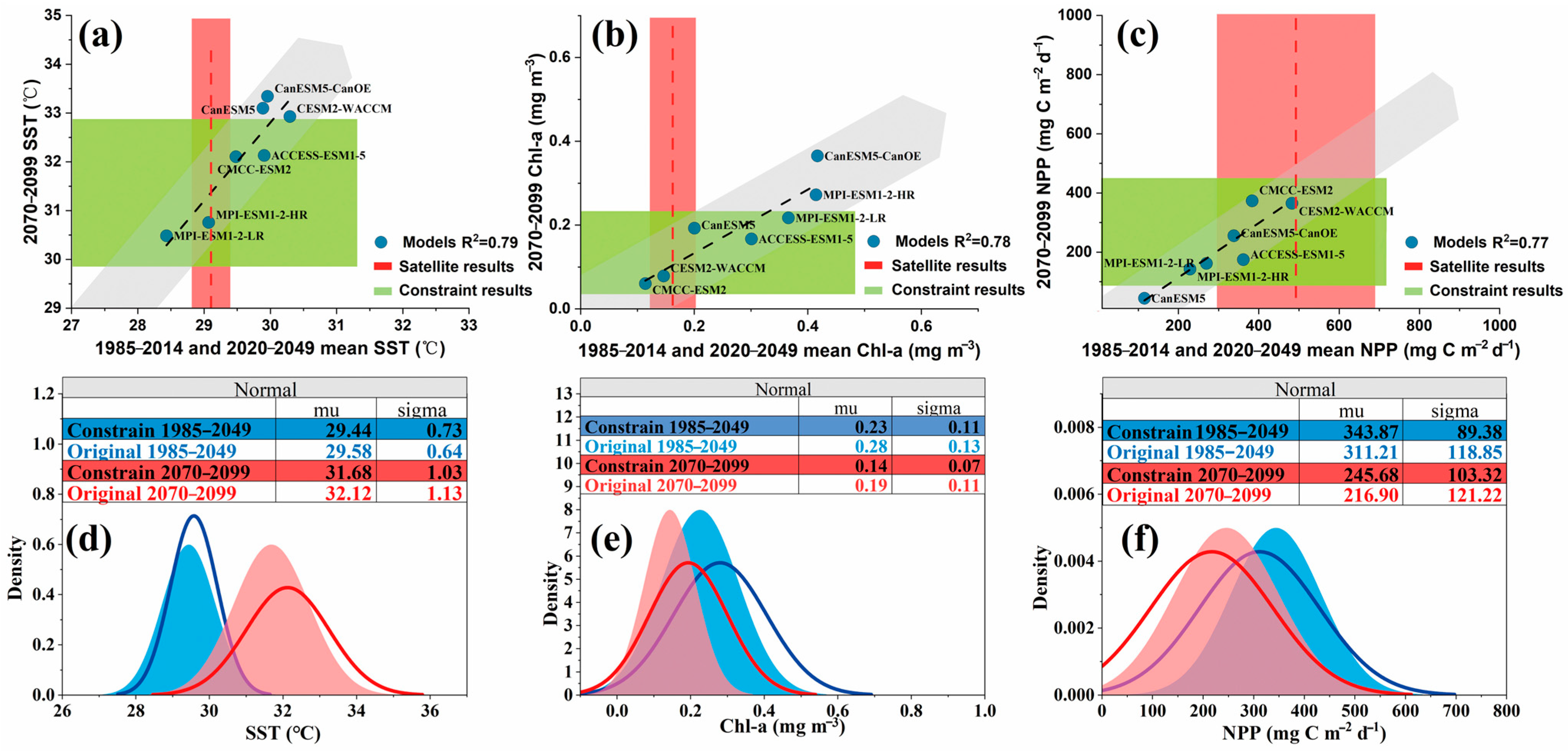
As shown in Figure 2a, we first examined the relationship between CMIP6 simulations for the present period and their corresponding projections for the end of the century, assuming a linear relationship. When a statistically significant correlation was identified, the present-day simulations and future projections were considered to be mutually constrained, with uncertainties quantified by the inter-model relative deviations. Meanwhile, as the remote sensing products have been regionally evaluated, satellite-derived estimates for the present period were regarded as reliable and used, together with their uncertainties quantified by the MRE values based on in situ observations, to constrain the CMIP6 simulations. CMIP6 models whose simulations at the present period are consistent with the satellite-derived estimates were then selected, and projections from these models were treated as the constrained future estimates. In practice, at first, for each CMIP6 model, its data within individual EEZ for the two periods (1985–2015 and 2020–2049) were extracted and spatiotemporally averaged. Then, we collected all CMIP6 models’ results and used the results from the two periods to establish a linear relationship. This relationship is then constrained by historical data from satellite observations, resulting in constrained estimates with reduced uncertainty for future climatological variables.

The calculations were as follows:

(1) For the marine environment indicator (SST, Chl-a, and NPP in this research), the satellite-derived Xsat (climatological mean) and δsat ($\mathrm{MRE} \mathrm{values}$) during 1998–2023 were calculated within each EEZ as:

$$\mathrm{Xsat} = {\displaystyle \frac{1}{\mathrm{N}}}{\sum }_{\mathrm{i} = 1}^{\mathrm{N}}\mathrm{Xsat},\mathrm{i}$$

(4)

$$\mathsf{\delta }\mathrm{sat}=\mathrm{MRE} \mathrm{values} \mathrm{based} \mathrm{on} \mathrm{filed} \mathrm{data} \mathrm{by} \mathrm{Equation} \left(1\right)$$

(5)

where $\mathrm{Xsat},\mathrm{i}$ is the satellite-derived regional mean results within each EEZ, N is the number of monthly data. These metrics represent the observed baseline conditions and natural variability from high-resolution satellite observations, which are later used to constrain CMIP6 model projections.

(2) A linear function was established to connect CMIP6 projections for 2070–2099 and the mean values from two earlier periods (1985–2014 and 2020–2049). The inter-model variability of CMIP6 projections in the 2070–2099 period (δcmip) was also calculated to represent the uncertainty of the linear function.

$${\mathrm{CMIP}6}_{2070–2099}=\mathrm{A} \times {\mathrm{mean}(\mathrm{CMIP}6}_{1985–2014} \mathrm{and} {\mathrm{CMIP}6}_{2020–2049})+\mathrm{B}$$

(6)

$$\mathsf{\delta }\mathrm{cmip}=\mathrm{abs}(\mathrm{Xcmip},\mathrm{i}-\mathrm{Xcmip}) \times 100\%/\mathrm{Xcmip}$$

(7)

where A and B denote the slope and intercept obtained from linear regression performed independently for each EEZ and all climate models under the chosen scenario (SSP1.26 or SSP5.85). $\mathrm{Xcmip},\mathrm{i}$ is the regional mean from each CMIP6 model-derived within different EEZs on the 2070–2099 period, and $\mathrm{Xcmip}$ is the ensemble mean from all available CMIP6 models on the 2070–2099 period.

(3) [Xsat × (1 − δsat), Xsat × (1 + δsat)] were used as a constraint range and applied to constrain the mean (${\mathrm{CMIP}6}_{1985–2014}$ and ${\mathrm{CMIP}6}_{2020–2049}$) in Equation (6) to achieve linear function constrained results: CMIP6 (Xsat × (1 − δsat)) and CMIP6 (Xsat × (1 + δsat)).

(4) The final scope of constrained results was then obtained as shown in Equation (8). For the ensemble of CMIP6 models, only those with predicted results on 2070–2099 falling within the above scope were adopted to form the constrained predictions.

$$\begin{array}{c}\left[\mathrm{m}\mathrm{i}\mathrm{n}\right(\mathrm{C}\mathrm{M}\mathrm{I}\mathrm{P}6 (\mathrm{X}\mathrm{s}\mathrm{a}\mathrm{t} \times (1 - \mathsf{\delta }\mathrm{s}\mathrm{a}\mathrm{t}\left)\right) \times (1 \pm \mathsf{\delta }\mathrm{c}\mathrm{m}\mathrm{i}\mathrm{p}), \mathrm{C}\mathrm{M}\mathrm{I}\mathrm{P}6 (\mathrm{X}\mathrm{s}\mathrm{a}\mathrm{t} \times (1+\mathsf{\delta }\mathrm{s}\mathrm{a}\mathrm{t}\left)\right) \times (1 \pm \mathsf{\delta }\mathrm{c}\mathrm{m}\mathrm{i}\mathrm{p})),\\ \mathrm{m}\mathrm{a}\mathrm{x}(\mathrm{C}\mathrm{M}\mathrm{I}\mathrm{P}6 (\mathrm{X}\mathrm{s}\mathrm{a}\mathrm{t} \times (1 - \mathsf{\delta }\mathrm{s}\mathrm{a}\mathrm{t})) \times (1 \pm \mathsf{\delta }\mathrm{c}\mathrm{m}\mathrm{i}\mathrm{p}), \mathrm{C}\mathrm{M}\mathrm{I}\mathrm{P}6 (\mathrm{X}\mathrm{s}\mathrm{a}\mathrm{t} \times (1+\mathsf{\delta }\mathrm{s}\mathrm{a}\mathrm{t})) \times (1 \pm \mathsf{\delta }\mathrm{c}\mathrm{m}\mathrm{i}\mathrm{p}\left)\right)]\end{array}$$

(8)

(5) To quantify the impact of the downscaling constraint, the statistical values (‘sigma’ of normal distribution fitting using OriginPro 2024 software) were compared before and after applying satellite-based adjustment. A reduced ‘sigma’ value indicates a decline in model uncertainty due to the satellite constraint.

The final downscaled products provide EEZ-scale refined projections of SST, Chl-a, and NPP changes between 1985 and 2014 and 2070–2099. These results reflect both the historical satellite-observed climatology and the long-term CMIP6 trends, thereby enhancing the regional relevance of projected marine environment changes for the SPICs.

3. Results and Discussion

3.1. Performance of the Satellite-Derived Data in Research Areas

3.1.1. Match-Up Between Satellite and in Situ Data

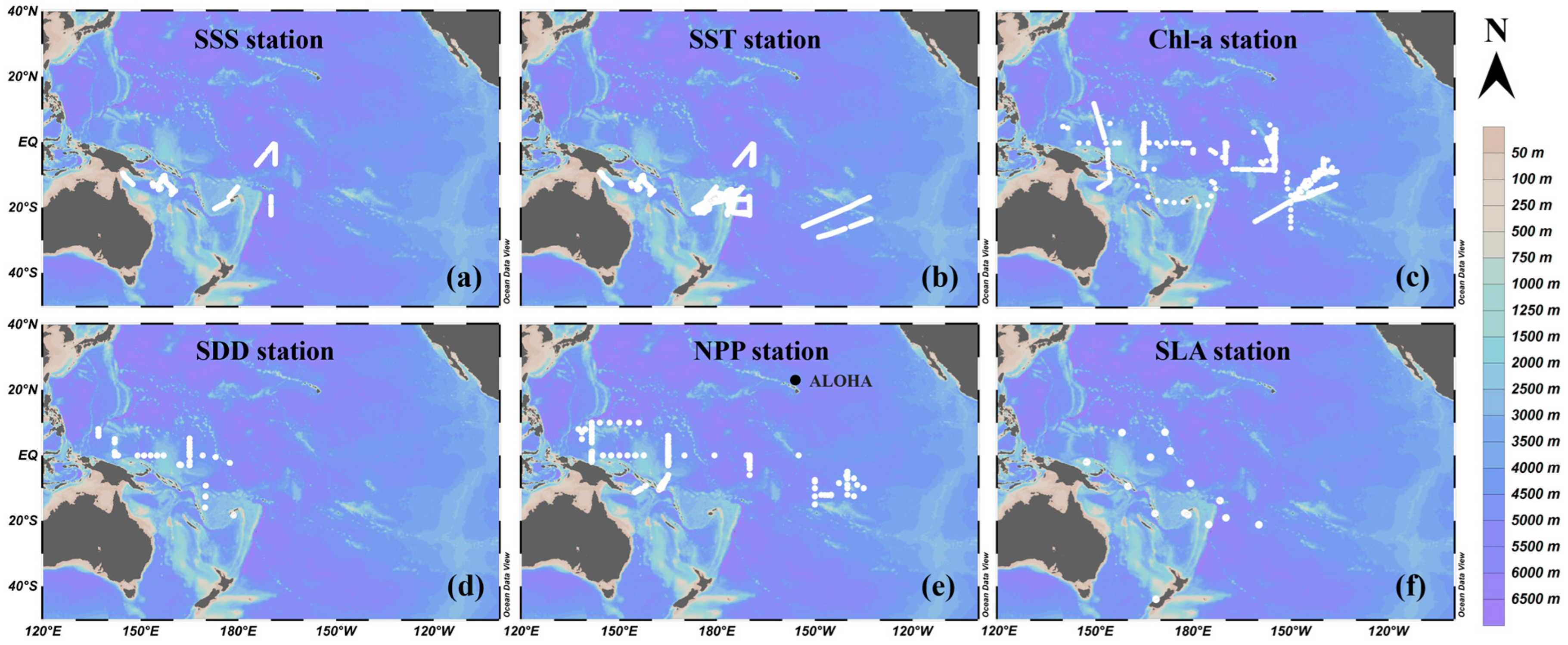
Unlike in situ measurements performed at fixed locations, satellite-derived pixels reflected an average state of the observation object in a certain square (depending on the production spatial resolution, e.g., 4 km) as the satellite passed by. During the performance evaluation process, a flexible spatiotemporal scale is required to balance the trade-off between maximizing the number of matched data points and ensuring the closest possible alignment between satellite and in situ observations in both time and space [46]. In this research, the field dataset was first filtered according to the boundaries of the EEZs of 12 SPICs. The satellite data were then matched with filtered in situ data at the nearest pixel on a monthly scale (Spatio-temporal matching schemes are shown in

Table 1. Spatio-temporal matching strategy of the multi-source remote sensing data.

Parameter (Units)	SSS (psu)	SST (°C)	Chl-a (mg m−3)	SDD (m)	NPP (mg C m−2 d−1)	SLA (m)
Temporal Resolution	monthly	monthly	monthly	monthly	monthly	monthly
Spatial Resolution	25 km	4 km	4 km	4 km	4 km	0.25°

). To assess the spatio-temporal representativeness of the limited matched-up in situ data, we compared the distribution of the matched-up in situ dataset against that of the entire in situ dataset over the study period and region. The station distribution of the matched-up in situ dataset stations is shown in Figure 3, the station distribution of the entire in situ dataset around the EEZs is shown in Supplementary Figure S1, and the comparison of the frequency distribution between the matched-up in situ data and the entire dataset is shown in Supplementary Figure S2. The frequency distributions of in situ SSS, SST, Chl-a, SDD, and NPP demonstrate that the matched-up data are reasonably distributed in the entire dataset (Supplementary Figure S2). This indicates that although the matched-up in situ data are sparse, they capture the key variation features in the entire in situ dataset.

3.1.2. Evaluation of Satellite-Derived Data

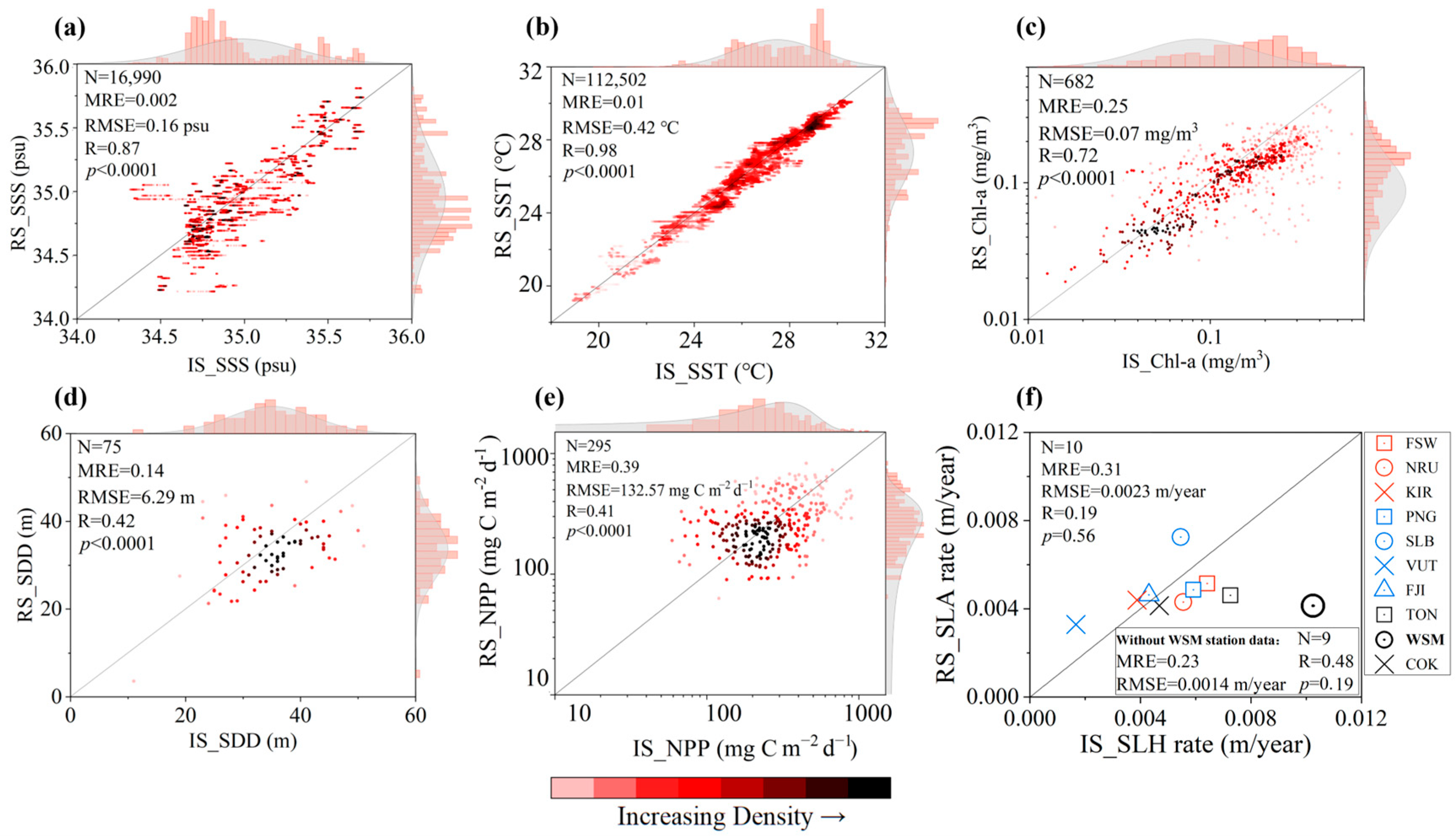
Figure 4 presents the comparison results of satellite and in situ data based on matched-up data pairs in the EEZs of the 12 SPICs. In general, satellites can serve as a reliable platform for monitoring marine environment changes in this region. Satellite-derived data showed the highest consistency with field observations for SST and SSS, with R of 0.98 and 0.87, and RMSE of 0.42 °C and 0.16 psu, respectively. Among the ecological indicators (Chl-a, SDD, and NPP), Chl-a performed best, exhibiting an MRE of 0.25 and an R of 0.72. For SDD and NPP, although the R values of match-up data decreased, significant correlations were still observed, with p-values < 0.0001 and MRE values < 0.40 (Figure 4d,e). For NPP, the evaluation of NPP model structure suitability using in situ observations as input supported the subsequent application of satellite-derived data in similar marine regions (Figure 4e). Based on field data at the ALOHA location, the satellite-derived NPP could perform relatively consistent variability with in situ observations, with MRE and RMSE values of 0.30 and 1.44 mg C m⁻³ d⁻¹, respectively (Supplementary Figure S3). For the hydrodynamic indicator (SLA or SLH), satellite-derived SLA showed consistent variability with in situ SLH observations over the same period. Across different EEZs in the study area, both in situ and satellite observations revealed a persistent sea level rise from 1993 to 2023 (Figure 5). Statistical analyses further supported the applicability of satellite-derived SLA in this region. Except for the WSM region, which exhibited a notable deviation, satellite-derived SLA captured sea level change rates consistent with those recorded by in situ SLH at other monitoring sites (Figure 4f). In fact, according to evaluation reports [36,37], the SLH records at WSM are considered unreliable due to station-related issues, such as earthquake impacts and land subsidence. Therefore, we also assessed the applicability of satellite-derived SLA in the region after excluding the potentially unreliable WSM station (Figure 4f). The validation metrics improved notably, with R increasing from 0.19 to 0.48 and RMSE decreasing from 0.0023 to 0.0014 m/year. Overall, the relative consistency between satellite data and in situ observations in this area supports research using satellite data to analyze changing characteristics of marine environment indicators across different EEZs.

3.1.3. National-Scale Uncertainty Analyses

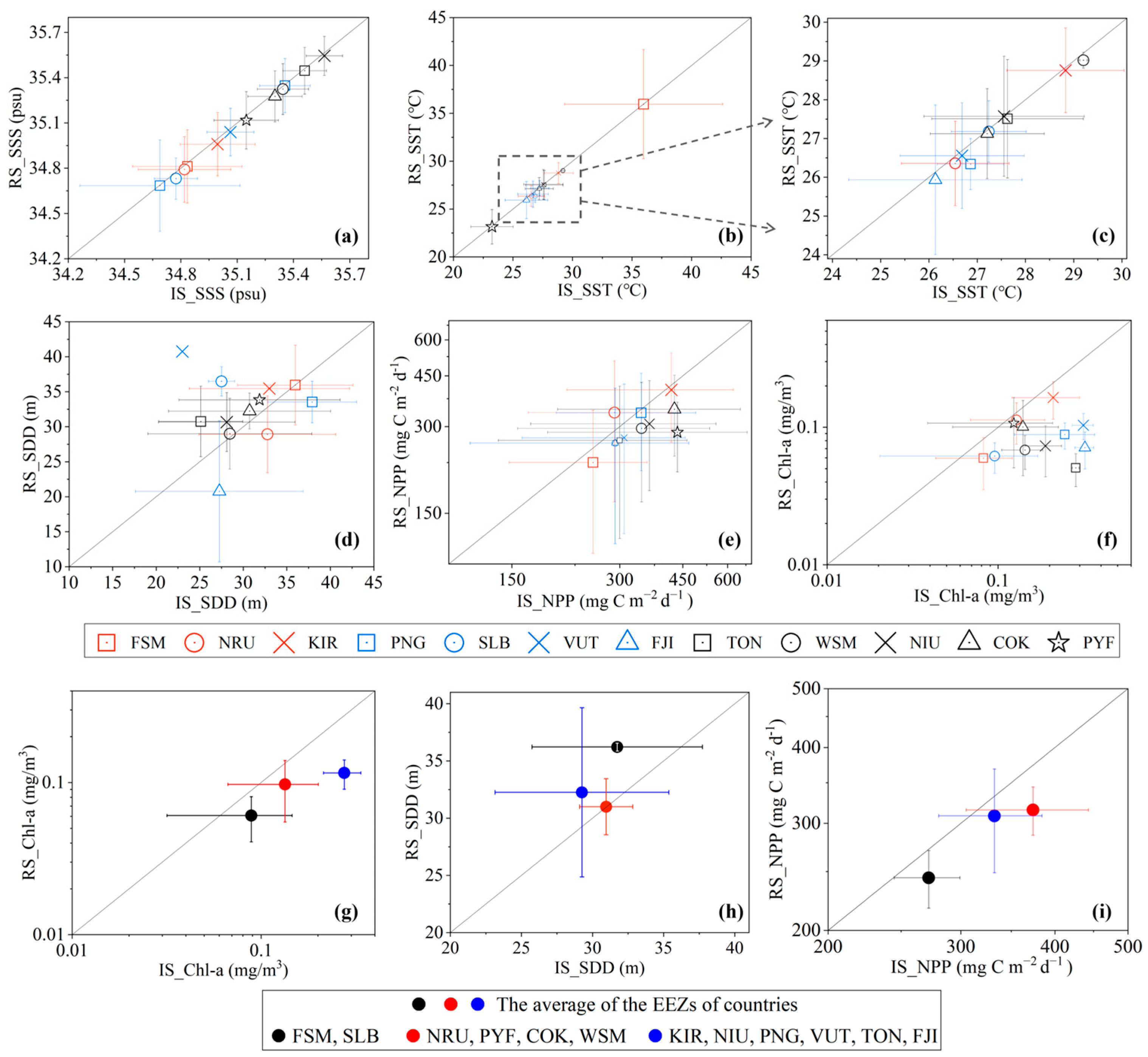
The uncertainty of satellite-derived data is associated with water constituent concentrations, exhibiting spatial variability [47]. To assess the applicability of satellite data for supporting EEZ-scale analyses in this region, we compared the median values within each EEZ based on all available matchup data. As shown in Figure 6, satellite-derived SSS and SST show high consistency with in situ observations across all EEZs, with MREs generally below 0.2% for SSS and 2% for SST. The EEZ-averaged errors were 0.62% (MRE) and 0.22 °C (RMSE) for SST, and 0.06% (MRE) and 0.03 psu (RMSE) for SSS, respectively. For SDD, the largest deviation was found in VUT, where MRE exceeded 50%. In other EEZs, SDD MREs remained below 30%. NPP exhibited larger intra-EEZ variability, but except for slightly higher deviations in PYF (34%), the MREs were generally within 20%, indicating acceptable consistency between satellite models and field observations. In contrast to the point-based assessment (Figure 4c), larger differences between satellite-derived and in situ Chl-a were found at the EEZ scale, with an overall MRE of 45%. In TON, FIJ, VUT, and PNG, MREs of Chl-a ranged between 60% and 80%. We further conducted three binned analyses for Chl-a, SDD, and NPP, using Chl-a thresholds of 0.1 and 0.2 mg m⁻³ as bin cutoffs. For SDD, MREs remained below 20% across bins. For Chl-a, in EEZs with median values below 0.2 mg m⁻³, satellite and in situ values showed reasonable consistency (MREs < 35%). However, when Chl-a exceeded 0.2 mg m⁻³, MRE increased to approximately 58%. As a comparison, NPP estimates (which depend on Chl-a as a model input) showed MRE within 20% in high-productivity waters (>400 mg C m⁻² d⁻¹) when in situ Chl-a data were used, highlighting the importance of improving Chl-a retrieval accuracy under high-biomass conditions.

Climatological Chl-a concentrations above 0.2 mg m⁻³ are associated with equatorial upwelling zones and nearshore waters (Section 3.2.1). However, in KIR, which is affected by equatorial upwelling, satellite and in situ Chl-a showed 22% MRE. Therefore, the discrepancies in Chl-a between satellite-derived and in situ data should be mainly concentrated in the coastal areas of this region. Previous studies have highlighted several key indicators affecting the regional accuracy of satellite-derived Chl-a products, including the accuracy of remote sensing reflectance (Rrs) inputs, the structure of the algorithms, and the spatiotemporal matchup methods [48,49]. Rrs accuracy is affected by both atmospheric correction [50,51] and radiative transfer conditions such as optical shallow depth and sun glint [47]. In our study region, although wildfires and volcanic activity can intermittently elevate terrestrial aerosols, sea-salt aerosols remain the dominant component of the regional aerosol composition [52]. Under these conditions, the current atmospheric correction algorithms employed for generating global satellite products can achieve satisfactory performance. Evaluations suggest that commonly used sensors (SeaWiFS, MODIS, MERIS) could produce accurate Rrs in clear waters within the study area [53,54], with uncertainties in the blue and green bands Rrs—used for Chl-a inversion—generally within 15% [55]. Optically shallow conditions, which are widespread in nearshore areas, likely constitute a significant source of error in satellite-derived Chl-a estimates. Given the 4 km spatial resolution of the global products employed in this study, pixels in nearshore regions may contain a mixture of optically shallow and deep waters, compromising the accuracy of satellite Chl-a. Satellite Chl-a products we selected generally rely on blue-to-green band ratio algorithms when Chl-a concentrations exceed 0.25 mg m⁻³ [56]. The fundamental assumption of global blue–green band ratio algorithms for ocean color remote sensing is that Chl-a absorbs strongly in the blue wavelengths while comparatively reflecting green wavelengths. Therefore, Chl-a concentration can be retrieved from the blue–green reflectance difference in the phytoplankton-dominated waters [57]. This assumption underpins classical global Chl-a algorithms (e.g., OC3, OC4), widely implemented in NASA’s ocean color products [56].

However, numerous studies have demonstrated that while the blue–green ratio correlates well with Chl-a in open ocean conditions, it frequently overestimates Chl-a concentrations in optically complex inland and coastal waters due to interference from colored dissolved organic matter (CDOM), non-algal particulates, and other constituents [58]. Unlike the global models’ assumption of optically deep conditions, spectrally selective bottom reflectance in shallow waters alters both the magnitude and shape of Rrs spectra, leading to substantial biases in satellite products, especially in the non-phytoplankton-dominated (Case-2) waters [59]. Furthermore, the IOCCG report [60] on ocean color algorithm performance emphasizes that strong blue absorption by CDOM and enhanced green scattering from suspended particles greatly violate the core assumptions of global algorithms, leading to substantial uncertainties in chlorophyll retrievals. Dekker et al. [61] showed that in different coastal zones of Australia and the Caribbean, due to significant disparities in water optical constituents (e.g., Chl-a, CDOM, suspended sediments) and substrate reflectance, the mean absolute error (MAE) between retrieved (e.g., Chl-a) results using global scale algorithms and in situ measurements could be 50% larger than that at the global scale. Aurin and Dierssen [62] provided a concrete example, indicating that in CDOM-dominated waters off the U.S. East Coast, standard ocean Chl-a algorithms (e.g., OC4) could overestimate Chl-a concentrations by 200–300% without adjustment. By incorporating regionally tuned optical parameters for correction, this bias could be constrained to within 30%.

In nearshore waters, the blue–green bands method often requires spectral adjustment (e.g., inclusion of red bands) or coefficient tuning to improve accuracy [63]. Evaluation in New Caledonia [64] indicated an underestimation of about 33% by blue-to-green ratio models, with similar underestimation recently also reported in Fiji [65]. Dupouy et al. [66] showed that for shallow coral reef lagoons in South Pacific islands (e.g., Fiji and New Caledonia), regional optimization of parameters in standard ocean color algorithms (e.g., OC3, OCI) or the development of region-specific algorithms could reduce the root mean square error (RMSE) of Chl-a estimation by approximately 20–30%. This finding provides a useful benchmark for our future work. Acknowledging the potentially higher uncertainty in nearshore regions, our results generally reinforce the reliability of satellite data for analyzing marine environment variability at the EEZ-scale in the SPICs. As research transitions from EEZ-scale to ecosystem-scale assessments, further enhancing the utility and service capacity of satellite-derived products will require several advances, e.g., strengthening in situ networks to provide sufficient data for accuracy assessment, refining satellite approaches by incorporating bottom reflectance effects [61,67], and developing regionally optimized models [62,66].

3.2. Variability of Marine Environment Indicators in EEZs

3.2.1. Climatological Intra-Annual Change

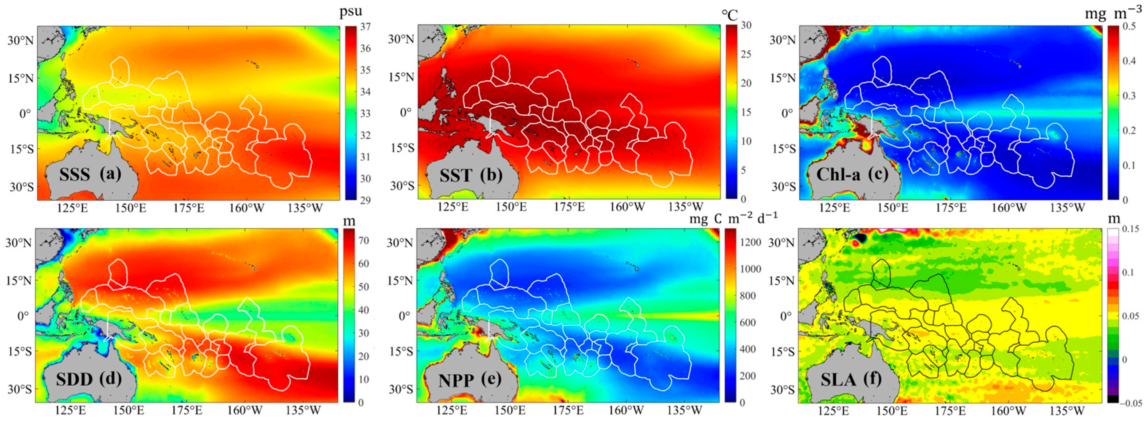
Figure 7 presents the climatological spatial distributions of SSS, SST, Chl-a, SDD, NPP, and SLA in the 12 EEZs of SPICs and their surrounding waters. In general, the marine environment in the study region exhibits apparent spatial variability, with distinct patterns observed across different indicators. SSS is relatively low (~34 psu) in the Northwestern part and the ocean near PNG. From Northwest to Southeast, SSS gradually increases from approximately 34 to 36 psu. In contrast, SST reaches its maximum (~30 °C) in the warm pool region (near PNG) and decreases to ~26 °C at latitudes above 15°S. Elevated Chl-a and NPP values are observed near island coasts and in areas influenced by equatorial upwelling, reaching up to 0.2 mg m⁻³ and 600 mg C m⁻² d⁻¹, respectively. In the oligotrophic gyre centers, Northwest and Southeast of the equator, Chl-a and NPP are generally below 0.1 mg m⁻³ and 300 mg C m⁻² d⁻¹. SDD exhibits an inverse relationship compared to Chl-a and NPP, being shallow (<40 m) in high-biomass zones and deep (up to ~70 m) in the low-biomass gyre centers. SLA demonstrates a latitudinal gradient, maintaining values of about 0.05 m near the equator and decreasing to about 0.03 m at latitudes greater than 15°S.

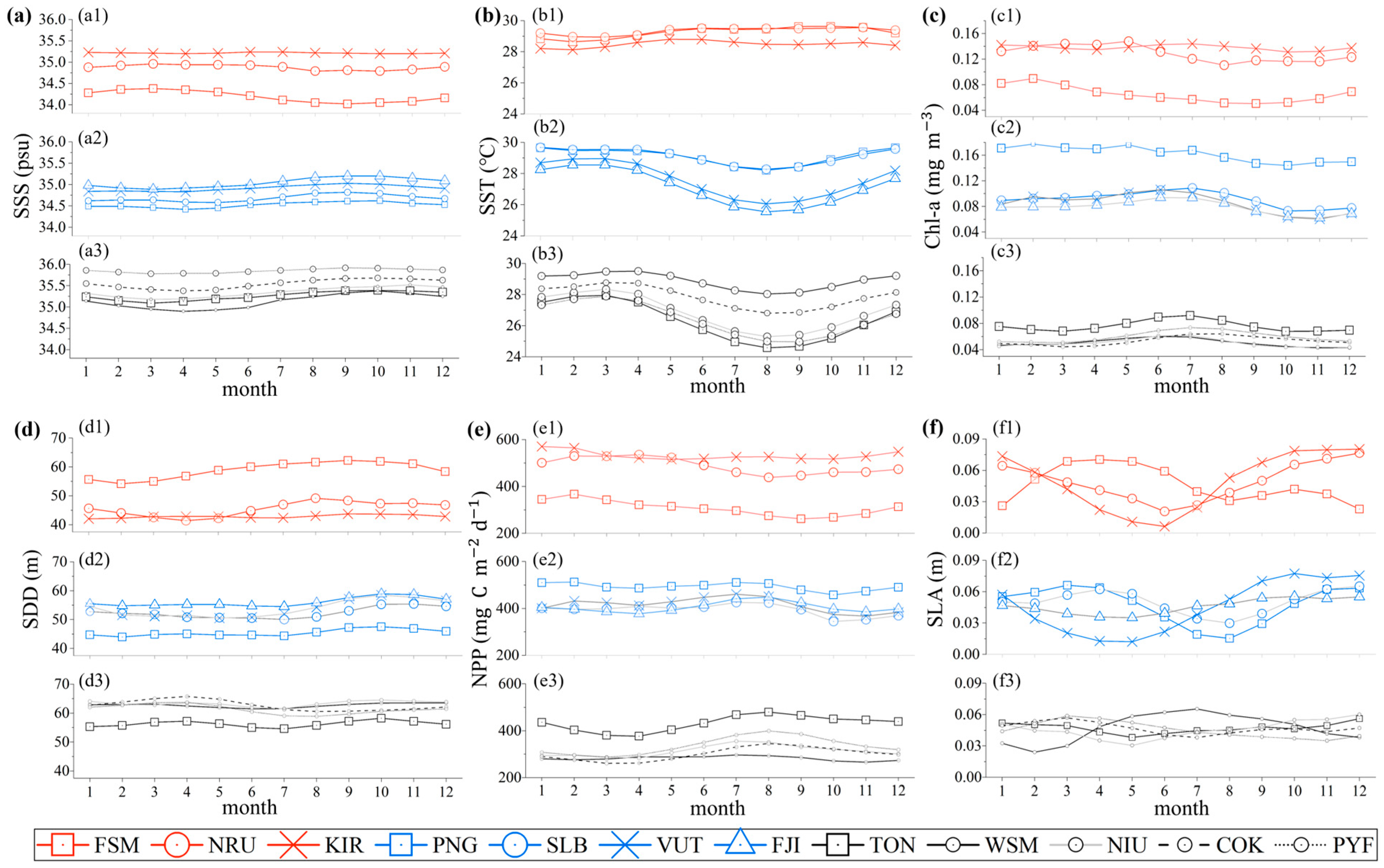
Figure 8 shows the climatological monthly variability of environment indicators across different EEZs, using regional median values. For the upwelling-influenced equatorial provinces (FSM, NRU, and KIR), SST remained high throughout the year, while intra-annual variability in SSS was limited. The relatively stable physical conditions supported weak seasonal variability in biological indicators (Chl-a and NPP), although Chl-a and NPP in KIR and NRU remained higher than those observed in FSM. In contrast, the Southeastern small island (TON, WSM, NIU, COK, and PYF) EEZs were characterized by high salinity levels (SSS > 35 psu) and pronounced seasonal SST fluctuations. SST was higher in December–April compared to in May–November, with seasonal amplitudes reaching up to 4 °C. Meanwhile, these regions generally exhibited low biological productivity, with Chl-a and NPP peaking in June–August, but their maximum values remained below 0.9 mg m⁻³ and 350 mg C m⁻² d⁻¹, respectively. Compared to the Southeastern small island EEZs, SST in the large island EEZs (PNG, SLB, VUT, and FJI) regions remained slightly higher, and SSS lower (SSS < 35 psu), with SST decreasing and SSS increasing during May–November. Chl-a and NPP in these areas were also higher than in the small island group, but still lower than in upwelling-influenced NRU and KIR EEZs. Across all EEZs, SDD exhibited an inverse relationship with Chl-a. In high-Chl-a regions, such as KIR and NRU, SDD values were typically less than 45 m, whereas in the oligotrophic Southeastern EEZs, SDD reached up to 65 m. Regarding SLA, Southeastern regions exhibited minimal seasonal variability (~0.03 m), while other EEZs displayed greater fluctuations with amplitudes around 0.05 m. It is worth noting that changes in environment variables do not completely align with the ecological provinces classification by Spalding et al. [33]. Distinct intra-annual variation patterns can be observed within the same ecological provinces, e.g., the changes in Chl-a (Figure 8c) and SLA (Figure 8f).

3.2.2. Inter-Annual Variability

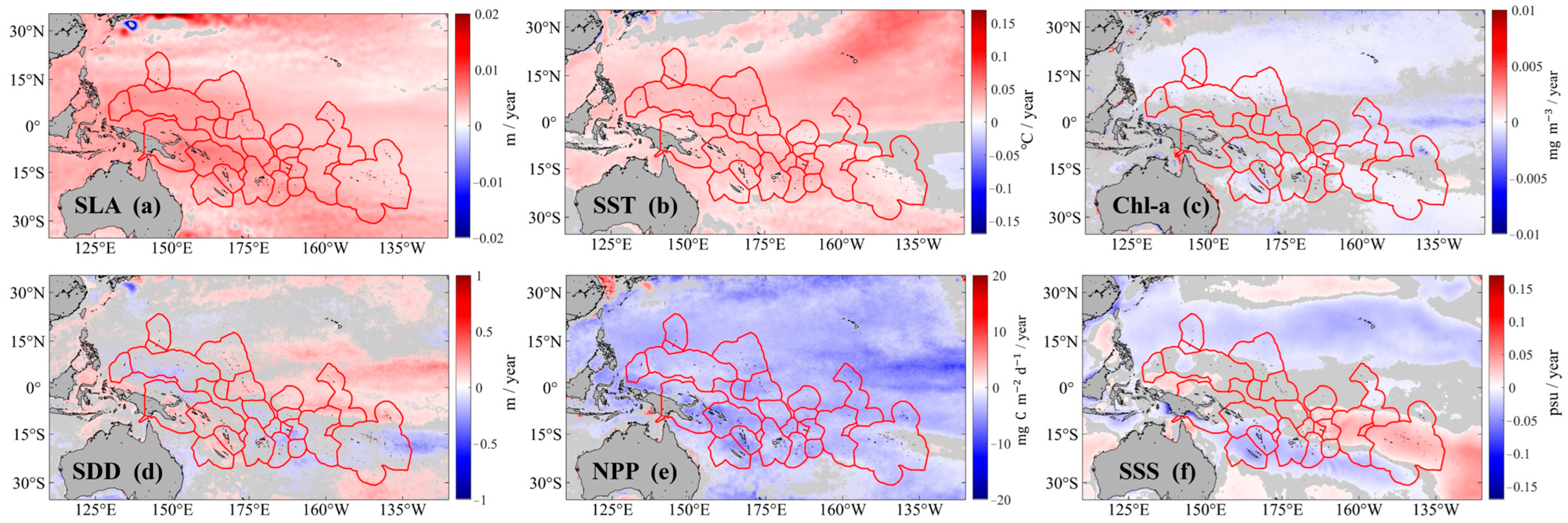
Over the past decades, all the 12 EEZs of SPICs have experienced a general increase in SST (1998–2023) (Figure 9b) and sea level rise (indicated by 1993–2023 SLA) (Figure 9a). In contrast, changes in biomass varied by region, with significant declines in Chl-a observed in several EEZs during 1998–2023. The reduction in Chl-a contributed to enhanced light penetration in the upper-layer waters, as indicated by increases in SDD. NPP—a key indicator for fisheries support—showed a declining change in all EEZs. Regarding SSS, an opposite change was observed over this region from 2010 to 2023. In the Eastern EEZs, SSS increased, whereas in the Western EEZs, surface waters became fresher, with decreasing SSS values.

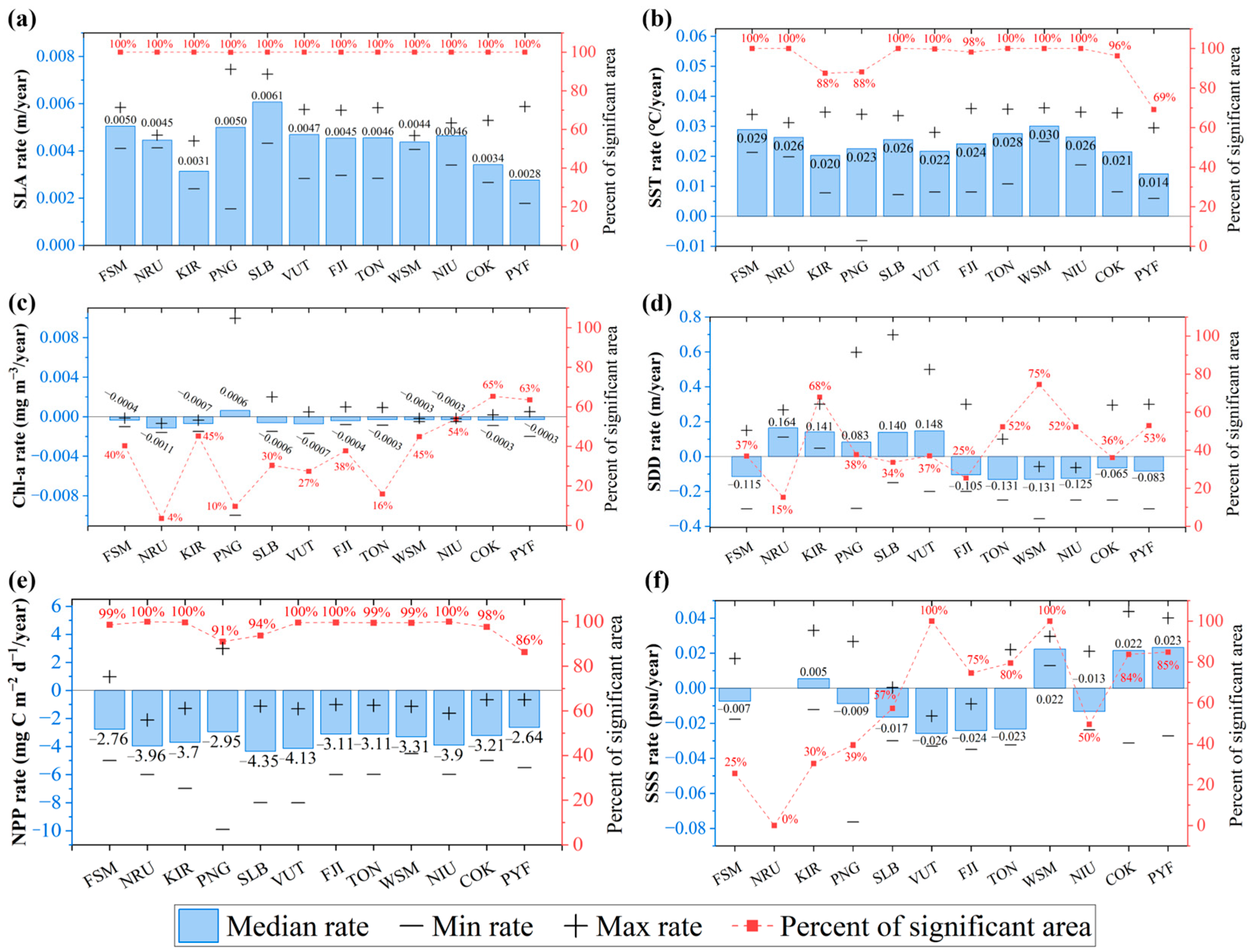
Figure 10 offers a national-scale perspective by illustrating the regional median, maximum, and minimum rates of change, together with the proportion of areas exhibiting statistically significant (p < 0.05) rates within each EEZ. Consistent with the patterns shown in Figure 9, both SLA and SST exhibited positive trends across all EEZs, with significant change areas covering over 100% and 70% of each EEZ, respectively. Among them, PYF recorded the smallest rates of increase in SLA (0.0028 m yr⁻¹) and SST (0.014 °C yr⁻¹), whereas SLB showed the highest rate of sea level rise (0.0061 m yr⁻¹). Relatively strong warming (>0.027 °C yr⁻¹) was also observed in FSM, TON, and WSM. Apart from PNG, where a slight increase in Chl-a was observed (0.0006 mg m⁻³ yr⁻¹), all other EEZs showed a decline in surface Chl-a. NRU exhibited the largest rate of decline (−0.0011 mg m⁻³ yr⁻¹), although this change was confined to only 4% of its EEZ. In contrast, NIU, COK, and PYF experienced significant and spatially extensive declines (over 50% of their EEZ area). While SDD increased in PNG, NRU, KIR, SLB, and VUT, other EEZs exhibited declining variability. As shown in Figure 10e, NPP declined across all EEZs. The largest declines occurred in NRU, SLB, VUT, and NIR, at approximately −4 mg C m⁻² d⁻¹ yr⁻¹. In contrast, the weakest declines occurred in FSM, PNG, and PYF, where rates were less than −3 mg C m⁻² d⁻¹ yr⁻¹. Regarding SSS (Figure 10f), no statistically significant change was detected in the NRU. Substantial declines in SSS were found in VUT, FJI, and TON (around −0.024 psu yr⁻¹), whereas WSM, COK, and PYF showed notable increases (~0.022 psu yr⁻¹). It is also worth noting that the considerable spatial heterogeneity in change rates was evident within individual EEZs. For variables such as SSS and SDD, both negative and positive rates co-occurred within the same EEZs. In particular, PNG exhibited the largest within-EEZ variability across all indicators, judging by the difference between the maximum and minimum values.

3.3. Evaluation of the CMIP6-Projected Results on EEZs Scale

3.3.1. CMIP6-Projected Results

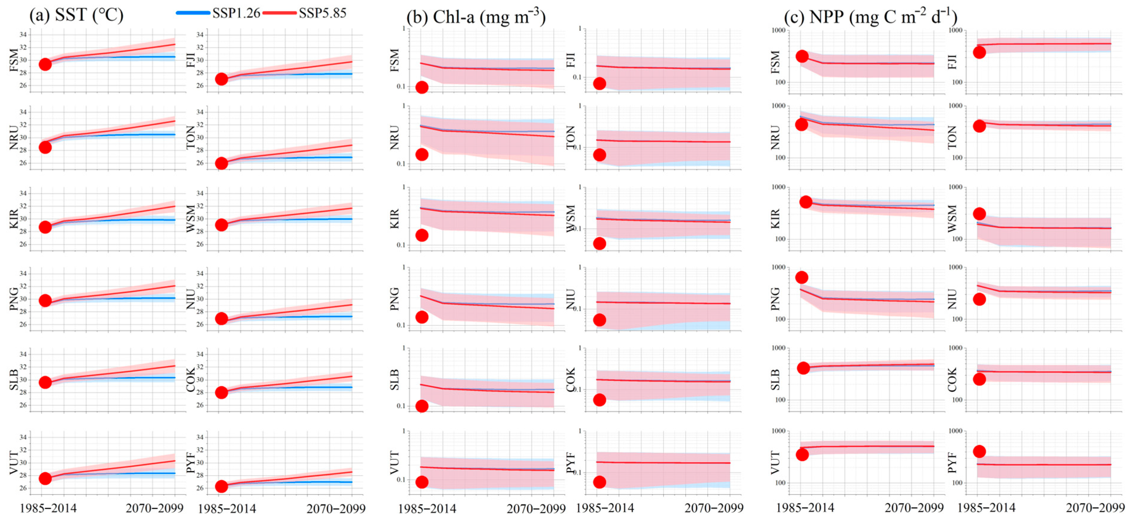
Consistent with current understanding based on local records, ocean warming enhances stratification and reduces biomass [11,23] CMIP6 projections widespread ocean warming and associated biomass decline in the study area by the end of the 21st century (Figure 11). The projected changes are closely linked to both the development scenarios and the indicators considered. SST increases faster under SSP5.85 than under the low-emission scenario SSP1.26. If the high-emission scenario SSP5.85 persists, SST in this region is expected to rise by approximately 3 °C by 2100. Even under SSP1.26, SST is projected to increase by about 1 °C. In contrast, due to overlapping uncertainty ranges, projected changes in Chl-a and NPP exhibit no significant differences between the two scenarios. On average, by 2100, the CMIP6-derived Chl-a and NPP are projected to decline by approximately 0.05 mg m⁻³ and 56 mg C m⁻² d⁻¹, respectively.

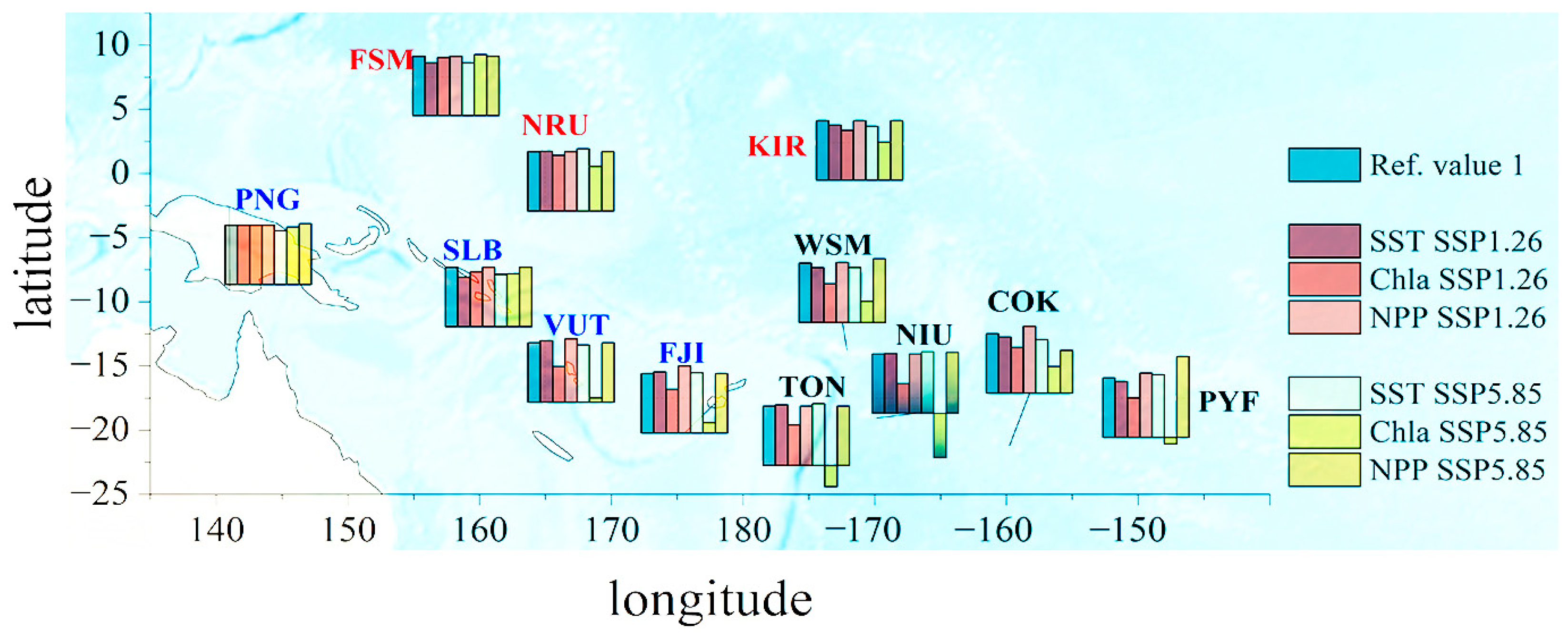
At the national scale, the largest projected changes in SST, Chl-a, and NPP are observed within the NRU EEZ, while the PYF EEZ is projected to maintain relatively stable ocean conditions (

Table 2. Changes (denoted by the symbol Δ) in SST (sea surface temperature, °C), Chl-a (chlorophyll-a, mg m⁻³), and NPP (net primary production, mg C m⁻² d⁻¹) within each EEZ (Exclusive Economic Zones) from 1984 to 2014 to 2070–2099 under the SSP1.26 and SSP5.85 scenarios.

	SSP1.26			SSP5.85
	ΔSST (°C)	ΔChl-a (mg m−3)	ΔNPP (mg C m−2 d−1)	ΔSST (°C)	ΔChl-a (mg m−3)	ΔNPP (mg C m−2 d−1)
FSM	1.11	−0.047	−79.63	3.05	−0.064	−89.02
NRU	1.42	−0.098	−190.81	3.46	−0.145	−246.70
KIR	1.36	−0.068	−104.07	3.38	−0.105	−152.99
PNG	1.06	−0.088	−136.86	3.02	−0.127	−156.76
SLB	1.02	−0.040	51.81	2.92	−0.063	71.20
VUT	0.90	−0.015	36.44	2.92	−0.027	27.36
FJI	0.97	−0.019	35.31	2.91	−0.023	30.69
TON	0.98	−0.016	−43.04	2.91	−0.014	−78.86
WSM	1.02	−0.023	−42.61	2.71	−0.028	−33.38
NIU	0.94	−0.012	−90.07	2.78	−0.012	−119.62
COK	0.89	−0.013	−17.21	2.55	−0.020	−14.51
PYF	0.65	−0.012	−6.75	2.19	−0.009	−3.60

The bold and underlined values indicate the regions exhibiting the largest and smallest changes for each indicator under a given scenario, respectively.

). In addition, when we used satellite-derived climatological results (1998–2023) as a reference, we found discrepancies between CMIP6 results (1984–2014) and satellite estimates across EEZs and indicators. For SST, the CMIP6 simulations exhibit overall consistency with satellite-based data. However, for Chl-a, CMIP6-derived results are higher than satellite estimates across all EEZs. In FSM, NRU, KIR, PNG, and WSM, the Chl-a discrepancies between CMIP6 and satellite results exceed the differences projected between SSP1.26 and SSP5.85. For NPP, CMIP6 results are higher than satellite values in PNG and PYF, but substantially lower in NRU and NIU. Considering that the satellite data have been validated against in situ observations in this region, these comparisons highlight the need for further evaluation of CMIP6 model applicability at the EEZ-scale within the SPICs region.

3.3.2. Re-Analysis of CMIP6 Projections with Satellite Results as Constraints

Taking the PNG region under SSP5.85 as an example (Figure 12), applying constraints would not alter the trends of rising SST and declining Chl-a and NPP. Meanwhile, applying constraints can reduce the uncertainty associated with projected SST, as evidenced by an approximate 8% decrease in the statistical fitting indicator (sigma, representing the width of the normal distribution). For Chl-a, the uncertainty in projections is expected to decrease by approximately 15% and 36% for the periods 1985–2049 and 2070–2099, respectively. Additionally, only one model fell outside the constraint boundaries for NPP; the adjustments nonetheless resulted in substantial reductions in uncertainty—approximately 25% for the period 1985–2019 and 15% for 2070–2099. When taking downscaling analysis at all EEZs, we observed that NRU and PYF remained, respectively, the regions with the largest and weakest projected changes in SST, Chl-a, and NPP (

Table 3. Changes (denoted by the symbol Δ) in SST (sea surface temperature, °C), Chl-a (chlorophyll-a, mg m⁻³), and NPP (net primary production, mg C m⁻² d⁻¹) within each EEZ (Exclusive Economic Zones) from 1984 to 2014 to 2070–2099 under the SSP1.26 and SSP5.85 scenarios after applying satellite constraints.

	SSP1.26			SSP5.85
	ΔSST (°C)	ΔChl-a (mg m−3)	ΔNPP (mg C m−2 d−1)	ΔSST (°C)	ΔChl-a (mg m−3)	ΔNPP (mg C m−2 d−1)
FSM	0.99	−0.046	−79.63 #	2.72	−0.066	−89.02 #
NRU	1.43	−0.092	−190.81 #	3.63 *	−0.109	−246.70 #
KIR	1.26	−0.057	−104.07 #	3.06	−0.067	−152.99 #
PNG	1.06 #	−0.088	−136.73	2.74	−0.123	−160.64
SLB	0.85	−0.037	51.81 #	2.57	−0.056	71.20 #
VUT	0.93	−0.009	38.91	2.81	−0.002	27.36 #
FJI	1.00	−0.014	39.86	2.95 #	−0.004	30.69 #
TON	1.00 *	−0.011	−43.04 #	3.03 *	0.005	−78.86 #
WSM	0.94 *	−0.015	−43.19	2.51	−0.010	−35.91
NIU	0.95 *	−0.006	−90.07 #	2.89 *	0.009	−122.63
COK	0.84	−0.010	−19.38	2.30	−0.009	−10.49
PYF	0.61	−0.008	−7.31	2.31	0.001	−4.90

The bold and underlined values indicate the regions exhibiting the largest and smallest changes for each indicator under a given scenario, respectively. Data marked with an ‘*’ indicate cases where no robust constraint relationship was found (r² < 0.5). Symbol ‘#’ means the constraints cannot filter out outlier CMIP6 models.

). Regarding the influence of constraints on the magnitude of change between 1985 and 2014 and 2070–2099 (Figure 13), we found that statistical downscaling showed minimal effect in FSM, PNG, and SLB. In contrast, for NRU and KIR, following statistical downscaling, the projected changes in Chl-a under SSP5.85 were weaker compared to the original estimates, as indicated by the ratio (<1) shown in Figure 13. Noticeable differences occurred in the Southeastern EEZs—VUT, FJI, WSM, and COK—where the magnitude of Chl-a changes under two scenarios was reduced after downscaling. For TON, NIU, and PYF, the downscaled projections even showed opposite trends for Chl-a under the SSP5.85 scenario, shifting from a decrease with the pre-downscaling estimates (Table 2) to an increase (Table 3).

Capabilities to obtain enough field data, the performance of CMIP6 models’ prediction for different indicators, and regional marine characteristics would account for the inter-country variability in downscaling analysis. As reported by SPREP [68], insufficient baseline data remain a major limitation for projecting climate impacts for small island developing nations (FSM, KIR, NRU, SLB, TON, and WSM). The CMIP6 models have shown varying degrees of skill in simulating oceanic conditions [69]. Compared with the high confidence in projected sea surface warming, the rates and magnitudes of biomass and NPP changes exhibit larger uncertainty and display substantial regional variability [5,70]. In addition, the inter-annual changes in Chl-a and NPP in the Southeastern oligotrophic EEZs were generally low (as shown in Figure 9). These weak signals may be masked by the CMIP6 model uncertainty and internal variability, thereby increasing the predicted uncertainty [71]. As reported by Schlunegger et al. [72], the time of emergence for statistically detectable Chl-a variability in CMIP6 simulations occurs approximately 20 years later in the Eastern marine regions than in the western parts of our study area. The EEZ, such as Nauru, are located in the equatorial Pacific, where marine ecosystems are strongly influenced by ENSO-driven variability, wind-driven upwelling, and thermocline depth fluctuations [73]. These processes lead to high natural variability in chlorophyll and primary productivity and increasing projected vulnerability [19,74]. In contrast, EEZs such as French Polynesia are primarily situated in the subtropical Southeastern Pacific, where oligotrophic conditions prevail, and large-scale circulation and thermodynamic forcing dominate [75]. The relatively stable physical environment results in lower natural variability and more stable ecosystem responses under future climate scenarios [76,77]. The same regional characteristics also explain why satellite data provide a stronger constraint on CMIP6 projections in Southeastern EEZs. Lower background variability enhances the signal-to-noise ratio, while satellite chlorophyll and primary productivity products generally perform better in open-ocean oligotrophic waters [18,19]. In addition, CMIP6 models exhibit more coherent systematic biases in subtropical oligotrophic regions, allowing satellite observations to more effectively discriminate between models [20]. As a result, satellite-based constraints lead to more pronounced adjustments of CMIP6 projections in Southeastern EEZs compared to equatorial or coastal-influenced regions. It should also be noted that our purpose is mainly to analyze the inter-country differences in CMIP6 performance before and after downscaling. To obtain convincing results of predicted change rates and magnitudes, a more comprehensive evaluation of the uncertainties in CMIP6 data within the specific EEZ regions is required [15]. In the absence of sufficient field data and given the substantial spatiotemporal mismatch between CMIP6 outputs and field observations, it is challenging to directly evaluate model performance at the EEZ scale. Our analysis reinforces confidence in using validated satellite data to assess CMIP6 performance at the EEZ scale in the PICTs region, as demonstrated in previous studies for other regions: the South China Sea [78] and the European marine [69].

The spatial resolution mismatch between satellite observations (4 km) and CMIP6 model outputs (∼1°) represents an inherent limitation for small island EEZ-scale analyses. Averaging coarse-resolution CMIP6 grid cells to the EEZ-scale inevitably smooths critical local environmental gradients captured by the satellite data, which are ecologically important for islands. As Evans et al. [21] demonstrated, for small island climates, the coarse resolution of the existing CMIP6 models is fundamentally insufficient. For most islands, higher-resolution (1 km-level) climate predictions need to be applied to capture the topography, coastline, and local circulation processes that determine the island’s climate, while islands surrounded by lagoons require even higher resolution [21,79]. However, this high resolution is only starting to become available [80,81]. In the future, when constructing observation constraints, it is advisable to consider resampling high-resolution satellite data to a scale that matches the CMIP6 model, thereby reducing the uncertainty caused by scale mismatch. On the other hand, as we discussed in Section 3.1.3, satellite-derived Chl-a and NPP products are known to be less reliable in high-biomass waters and shallow coastal regions, where optical complexity, bottom reflectance, and non-algal particles can introduce additional uncertainties [60,61,62]. We therefore emphasize that the satellite-based constraint could be effective when satellite retrieval algorithms have been validated and associated uncertainties are lower.

4. Conclusions

Focusing on the national-scale requirements for assessing marine environment changes in the SPICs region, this study evaluated the applicability of satellite-derived datasets in representing the variability of key oceanic indicators that are of regional concern. The main findings are as follows:

(1)

Validation results support our confidence in using current satellite products (SST, SSS, SDD, Chl-a, NPP, and SLA) to conduct EEZ-scale assessments. Further investigation is required to assess their applicability at nearshore or community–ecosystem scales, where increased local optical complexity and dynamic processes may introduce greater uncertainties.

(2)

All 12 EEZs experienced seawater warming and sea-level rise, while Chl-a, NPP, SDD, and SSS exhibited within-EEZ heterogeneity. Among the study areas, Papua New Guinea exhibited the largest within-EEZ inter-annual variability across the analyzed indicators.

(3)

Satellite-derived data would help to constrain the uncertainty of CMIP6 model projections in the SPICs, subject to the accuracy of the satellite products. By 2100, Nauru EEZ is projected to be the most vulnerable, while French Polynesia is expected to maintain relatively stable oceanic conditions among all 12 EEZs. In contrast, significant changes are exhibited between unconstrained and constrained CMIP6 projections in the Southeastern EEZs.

Overall, this study highlights the essential role of satellite observations as both monitoring tools and model constraints. The findings could offer actionable national-scale evidence for the application of satellite data in regional climate adaptation planning, sustainable marine resource management, and policy development in the SPICs.

References

1. Office of the UN Resident Coordinator. United Nations Pacific Strategy 2018–2022: A Multi-Country Sustainable Development Framework in the Pacific Region; United Nations: New York, NY, USA, 2017. [Google Scholar]
2. Thakur, R. Introduction to the South Pacific. In The South Pacific: Problems, Issues and Prospects; Palgrave Macmillan: London, UK, 1991; pp. 1–33. [Google Scholar]
3. Devlin, M.J.; Lyons, B.P.; Johnson, J.E.; Hills, J.M. The tropical Pacific Oceanscape: Current issues, solutions and future possibilities. Mar. Pollut. Bull. 2021, 166, 112181. [Google Scholar] [CrossRef]
4. Hay, J.E.; Mimura, N. Vulnerability, Risk and Adaptation Assessment Methods in the Pacific Islands Region: Past approaches, and considerations for the future. Sustain. Sci. 2013, 8, 391–405. [Google Scholar] [CrossRef]
5. IPCC. Summary for Policymakers. In Climate Change 2022: Impacts, Adaptation, and Vulnerability. Contribution of Working Group II to the Sixth Assessment Report of the Intergovernmental Panel on Climate Change; Pörtner, H.-O., Roberts, D.C., Tignor, M., Poloczanska, E., Mintenbeck, K., Alegría, A., Craig, M., Langsdorf, S., Löschke, S., Möller, V., et al., Eds.; Cambridge University Press: Cambridge, UK; New York, NY, USA, 2022; pp. 3–33. [Google Scholar]
6. Marra, J.J.; Gooley, G.; Johnson, M.-V.V.; Keener, V.W.; Kruk, M.; McGree, S.; Potemra, J.T.; Warrick, O. Pacific Islands Climate Change Monitor: 2021. In The Pacific Islands-Regional Climate Centre (PI-RCC) Network Report to the Pacific Islands Climate Service (PICS) Panel and Pacific Meteorological Council (PMC); PI-RCC: Geneva, Switzerland, 2022. [Google Scholar]
7. Barnett, J. Adapting to Climate Change in Pacific Island Countries: The Problem of Uncertainty. World Dev. 2001, 29, 977–993. [Google Scholar] [CrossRef]
8. WMO. State of the Climate in the South-West Pacific; 1356; World Meteorological Organization (WMO): Geneva, Switzerland, 2024; p. 31. [Google Scholar]
9. Keener, V.; Helweg, D.; Asam, S.; Balwani, S.; Burkett, M.; Fletcher, C.; Giambelluca, T.; Grecni, Z.; Nobrega-Olivera, M.; Polovina, J.; et al. Hawai’i and US-Affiliated Pacific Islands; U.S. Global Change Research Program: Washington, DC, USA, 2018.
10. Masson-Delmotte, V.; Zhai, P.; Pörtner, H.-O.; Roberts, D.; Skea, J.; Shukla, P.R.; Pirani, A.; Moufouma-Okia, W.; Péan, C.; Pidcock, R. Global Warming of 1.5 °C; IPCC: Geneva, Switzerland, 2018; Volume 1, pp. 43–50. [Google Scholar]
11. SPREP. SPREP Annual Report: 2023; 45826; Secretariat of the Pacific Regional Environment Programme (SPREP): Apia, Samoa, 2024; p. 92. [Google Scholar]
12. Benjamin, L.; Thomas, A. 1.5 To Stay Alive? AOSIS and the Long Term Temperature Goal in the Paris Agreement. Environ. Sci. Political Sci. 2016, 10, 277–282. [Google Scholar] [CrossRef]
13. Goldberg, W.M. An introduction to the tropical Pacific and types of Pacific Islands. In The Geography, Nature and History of the Tropical Pacific and Its Islands; Springer: Berlin/Heidelberg, Germany, 2017; pp. 1–38. [Google Scholar]
14. McGree, S.; Smith, G.; Chandler, E.; Harold, N.; Begg, Z.; Kuleshov, Y.; Malsale, P.; Ritman, M. Climate Change in the Pacific 2022: Historical and Recent Variability, Extremes and Change; Pacific Community (SPC): Suva, Fiji, 2022. [Google Scholar]
15. Dhage, L.; Widlansky, M.J. Assessment of 21st Century Changing Sea Surface Temperature, Rainfall, and Sea Surface Height Patterns in the Tropical Pacific Islands Using CMIP6 Greenhouse Warming Projections. Earth’s Future 2022, 10, e2021EF002524. [Google Scholar] [CrossRef]
16. Keener, V.W.; Grecni, Z.N.; Moser, S.C. Accelerating Climate Change Adaptive Capacity Through Regional Sustained Assessment and Evaluation in Hawai‘i and the U.S. Affiliated Pacific Islands. Front. Clim. 2022, 4, 869760. [Google Scholar] [CrossRef]
17. Zhong, S.; Ying, J.; Collins, M. Sources of Uncertainty in the Time of Emergence of Tropical Pacific Climate Change Signal: Role of Internal Variability. J. Clim. 2023, 36, 2535–2549. [Google Scholar] [CrossRef]
18. Wills, R.C.J.; Dong, Y.; Proistosecu, C.; Armour, K.C.; Battisti, D.S. Systematic Climate Model Biases in the Large-Scale Patterns of Recent Sea-Surface Temperature and Sea-Level Pressure Change. Geophys. Res. Lett. 2022, 49, e2022GL100011. [Google Scholar] [CrossRef]
19. Tagliabue, A.; Kwiatkowski, L.; Bopp, L.; Butenschön, M.; Cheung, W.; Lengaigne, M.; Vialard, J. Persistent Uncertainties in Ocean Net Primary Production Climate Change Projections at Regional Scales Raise Challenges for Assessing Impacts on Ecosystem Services. Front. Clim. 2021, 3, 738224. [Google Scholar] [CrossRef]
20. Kwiatkowski, L.; Bopp, L.; Aumont, O.; Ciais, P.; Cox, P.M.; Laufkötter, C.; Li, Y.; Séférian, R. Emergent constraints on projections of declining primary production in the tropical oceans. Nat. Clim. Change 2017, 7, 355–358. [Google Scholar] [CrossRef]
21. Evans, J.P.; Belmadani, A.; Menkes, C.; Stephenson, T.; Thatcher, M.; Gibson, P.B.; Peltier, A. Higher-resolution projections needed for small island climates. Nat. Clim. Change 2024, 14, 668–670. [Google Scholar] [CrossRef]
22. Amani, M.; Ghorbanian, A.; Asgarimehr, M.; Yekkehkhany, B.; Moghimi, A.; Jin, S.; Naboureh, A.; Mohseni, F.; Mahdavi, S.; Layegh, N.F. Remote Sensing Systems for Ocean: A Review (Part 1: Passive Systems). IEEE J. Sel. Top. Appl. Earth Obs. Remote Sens. 2022, 15, 210–234. [Google Scholar] [CrossRef]
23. Zhu, B.; Bai, Y.; He, X.; Chen, X.; Li, T.; Gong, F. Long-Term Changes in the Land–Ocean Ecological Environment in Small Island Countries in the South Pacific: A Fiji Vision. Remote Sens. 2021, 13, 3740. [Google Scholar] [CrossRef]
24. Wang, W.; Zhou, C.; Shao, Q.; Mulla, D.J. Remote sensing of sea surface temperature and chlorophyll-a: Implications for squid fisheries in the north-west Pacific Ocean. Int. J. Remote Sens. 2010, 31, 4515–4530. [Google Scholar] [CrossRef]
25. Hsu, T.; Chang, Y.; Lee, M.; Wu, R.-F.; Hsiao, S. Predicting Skipjack Tuna Fishing Grounds in the Western and Central Pacific Ocean Based on High-Spatial-Temporal-Resolution Satellite Data. Remote Sens. 2021, 13, 861. [Google Scholar] [CrossRef]
26. Marrack, L.; Wiggins, C.; Marra, J.J.; Genz, A.; Most, R.; Falinski, K.; Conklin, E. Assessing the spatial–temporal response of groundwater-fed anchialine ecosystems to sea-level rise for coastal zone management. Aquat. Conserv. Mar. Freshw. Ecosyst. 2021, 31, 853–869. [Google Scholar] [CrossRef]
27. Kim, H.; Timmermann, A.; Lee, S.-S.; Schloesser, F. Rainfall and Salinity Effects on Future Pacific Climate Change. Earth’s Future 2023, 11, e2022EF003457. [Google Scholar] [CrossRef]
28. Jiang, Z.; Song, Z.; Bai, Y.; He, X.; Yu, S.; Zhang, S.; Gong, F. Remote sensing of global sea surface pH based on massive underway data and machine learning. Remote Sens. 2022, 14, 2366. [Google Scholar] [CrossRef]
29. Huang, B.; Liu, C.; Banzon, V.; Freeman, E.; Graham, G.; Hankins, B.; Smith, T.; Zhang, H.-M. Improvements of the Daily Optimum Interpolation Sea Surface Temperature (DOISST) Version 2.1. J. Clim. 2021, 34, 2923–2939. [Google Scholar] [CrossRef]
30. Mortreux, C.; Jarillo, S.; Barnett, J.; Waters, E. Climate change and migration from atolls? No evidence yet. Curr. Opin. Environ. Sustain. 2023, 60, 101234. [Google Scholar] [CrossRef]
31. IOCCG. Uncertainties in Ocean Colour Remote Sensing; International Ocean Colour Coordinating Group (IOCCG): Dartmouth, NS, Canada, 2019; p. 163. [Google Scholar]
32. Powers, M.; Begg, Z.; Smith, G.; Miles, E. Lessons From the Pacific Ocean Portal: Building Pacific Island Capacity to Interpret, Apply, and Communicate Ocean Information. Front. Mar. Sci. 2019, 6, 476. [Google Scholar] [CrossRef]
33. Spalding, M.D.; Fox, H.E.; Allen, G.R.; Davidson, N.; Ferdaña, Z.A.; Finlayson, M.; Halpern, B.S.; Jorge, M.A.; Lombana, A.; Lourie, S.A.; et al. Marine Ecoregions of the World: A Bioregionalization of Coastal and Shelf Areas. BioScience 2007, 57, 573–583. [Google Scholar] [CrossRef]
34. Valente, A.; Sathyendranath, S.; Brotas, V.; Groom, S.; Grant, M.; Taberner, M.; Antoine, D.; Arnone, R.; Balch, W.M.; Barker, K. A compilation of global bio-optical in situ data for ocean-colour satellite applications–version two. Earth Syst. Sci. Data 2019, 11, 1037–1068. [Google Scholar] [CrossRef]
35. Karl, D.M.; Letelier, R.M.; Bidigare, R.R.; Björkman, K.M.; Church, M.J.; Dore, J.E.; White, A.E. Seasonal-to-decadal scale variability in primary production and particulate matter export at Station ALOHA. Prog. Oceanogr. 2021, 195, 102563. [Google Scholar] [CrossRef]
36. ADB. Sea-Level Change in the Pacific Islands Region: A Review of Evidence to Inform Asian Development Bank Guidance on Selecting Sea-Level Projections for Climate Risk and Adaptation Assessments; ADB: Manila, Philippines, 2022. [Google Scholar]
37. Hills, J.; Moore, T.; Goyet, S.; Singh, A.; Brodie, G.; Pringle, P.; Seuseu, S.; Straza, T.; Buckley, P.; Townhill, B.; et al. Pacific Marine Climate Change Report Card December 2018; Commonwealth Marine Economies Programme; UK’s Centre for Environment: Wallingford, UK, 2018. [Google Scholar]
38. He, X.; Pan, D.; Bai, Y.; Wang, T.; Chen, C.-T.A.; Zhu, Q.; Hao, Z.; Gong, F. Recent changes of global ocean transparency observed by SeaWiFS. Cont. Shelf Res. 2017, 143, 159–166. [Google Scholar] [CrossRef]
39. Yu, S.; Bai, Y.; He, X.; Gong, F.; Li, T. A new merged dataset of global ocean chlorophyll-a concentration for better trend detection. Front. Mar. Sci. 2023, 10, 1051619. [Google Scholar] [CrossRef]
40. Behrenfeld, M.J.; Falkowski, P.G. Photosynthetic rates derived from satellite-based chlorophyll concentration. Limnol. Oceanogr. 1997, 42, 1–20. [Google Scholar] [CrossRef]
41. Wang, K.; Cai, W.-J.; Chen, J.; Kirchman, D.; Wang, B.; Fan, W.; Huang, D. Climate and Human-Driven Variability of Summer Hypoxia on a Large River-Dominated Shelf as Revealed by a Hypoxia Index. Front. Mar. Sci. 2021, 8, 634184. [Google Scholar] [CrossRef]
42. Leroux, M.-D.; Bonnardot, F.; Somot, S.; Alias, A.; Kotomangazafy, S.; Ridhoine, A.-O.S.; Veerabadren, P.; Amélie, V. Advancing climate services for vulnerable islands in the Southwest Indian Ocean: A combined approach of statistical and dynamical Cmip6 downscaling. Clim. Serv. 2024, 34, 100491. [Google Scholar] [CrossRef]
43. Brient, F. Reducing Uncertainties in Climate Projections with Emergent Constraints: Concepts, Examples and Prospects. Adv. Atmos. Sci. 2020, 37, 1–15. [Google Scholar] [CrossRef]
44. Hall, A.; Cox, P.; Huntingford, C.; Klein, S. Progressing emergent constraints on future climate change. Nat. Clim. Change 2019, 9, 269–278. [Google Scholar] [CrossRef]
45. Tokarska, K.B.; Stolpe, M.B.; Sippel, S.; Fischer, E.M.; Smith, C.J.; Lehner, F.; Knutti, R. Past warming trend constrains future warming in CMIP6 models. Sci. Adv. 2020, 6, eaaz9549. [Google Scholar] [CrossRef]
46. Bailey, S.W.; Werdell, P.J. A multi-sensor approach for the on-orbit validation of ocean color satellite data products. Remote Sens. Environ. 2006, 102, 12–23. [Google Scholar] [CrossRef]
47. Zhang, M.; Ibrahim, A.; Franz, B.A.; Ahmad, Z.; Sayer, A.M. Estimating pixel-level uncertainty in ocean color retrievals from MODIS. Opt. Express 2022, 30, 31415–31438. [Google Scholar] [CrossRef]
48. Hu, S.; Zhou, W.; Wang, G.; Cao, W.; Xu, Z.; Liu, H.; Wu, G.; Zhao, W. Comparison of satellite-derived phytoplankton size classes using in-situ measurements in the South China Sea. Remote Sens. 2018, 10, 526. [Google Scholar] [CrossRef]
49. Blondeau-Patissier, D.; Gower, J.F.R.; Dekker, A.G.; Phinn, S.R.; Brando, V.E. A review of ocean color remote sensing methods and statistical techniques for the detection, mapping and analysis of phytoplankton blooms in coastal and open oceans. Prog. Oceanogr. 2014, 123, 123–144. [Google Scholar] [CrossRef]
50. Clark, D.K.; Gordon, H.R.; Voss, K.J.; Ge, Y.; Broenkow, W.; Treess, C. Validation of atmospheric correction over the oceans. J. Geophys. Res. Atmos. 1997, 102, 17209–17217. [Google Scholar] [CrossRef]
51. Zibordi, G.; Holben, B.; Slutsker, I.; Giles, D.; D’Alimonte, D.; Mélin, F.; Berthon, J.F.; Vandemark, D.; Feng, H.; Schuster, G.; et al. AERONET-OC: A network for the validation of ocean color primary products. J. Atmos. Ocean. Technol. 2009, 26, 1634–1651. [Google Scholar] [CrossRef]
52. Isaza, A.; Hilly, J.; Kay, M.; Prasad, A.; Dansie, A. Atmospheric aerosols in the South Pacific: A regional baseline and characterization of aerosol fractions. Atmos. Environ. 2025, 346, 121048. [Google Scholar] [CrossRef]
53. Wei, J.; Lee, Z.; Shang, S. A system to measure the data quality of spectral remote-sensing reflectance of aquatic environments. J. Geophys. Res. Ocean. 2016, 121, 8189–8207. [Google Scholar] [CrossRef]
54. Mélin, F.; Sclep, G.; Jackson, T.; Sathyendranath, S. Uncertainty estimates of remote sensing reflectance derived from comparison of ocean color satellite data sets. Remote Sens. Environ. 2016, 177, 107–124. [Google Scholar] [CrossRef]
55. Hu, C.; Feng, L.; Lee, Z. Uncertainties of SeaWiFS and MODIS remote sensing reflectance: Implications from clear water measurements. Remote Sens. Environ. 2013, 133, 168–182. [Google Scholar] [CrossRef]
56. O’Reilly, J.E.; Werdell, P.J. Chlorophyll algorithms for ocean color sensors—OC4, OC5 & OC6. Remote Sens. Environ. 2019, 229, 32–47. [Google Scholar] [CrossRef]
57. Morel, A.; Prieur, L. Analysis of variations in ocean color. Limnol. Oceanogr. 1977, 22, 709–722. [Google Scholar] [CrossRef]
58. Pahlevan, N.; Smith, B.; Schalles, J.; Binding, C.; Cao, Z.; Ma, R.; Alikas, K.; Kangro, K.; Gurlin, D.; Hà, N.; et al. Seamless retrievals of chlorophyll-a from Sentinel-2 (MSI) and Sentinel-3 (OLCI) in inland and coastal waters: A machine-learning approach. Remote Sens. Environ. 2020, 240, 111604. [Google Scholar] [CrossRef]
59. Lee, Z.; Hu, C.; Casey, B.; Shang, S.; Dierssen, H.; Arnone, R. Global shallow-water bathymetry from satellite ocean color data. Eos Trans. Am. Geophys. Union 2010, 91, 429–430. [Google Scholar] [CrossRef]
60. IOCCG. Remote Sensing of Ocean Colour in Coastal, and Other Optically-Complex, Waters; Reports of the International Ocean-Colour Coordinating Group; IOCCG: Dartmouth, NS, Canada, 2000. [Google Scholar]
61. Dekker, A.G.; Phinn, S.R.; Anstee, J.; Bissett, P.; Brando, V.E.; Casey, B.; Fearns, P.; Hedley, J.; Klonowski, W.; Lee, Z.P.; et al. Intercomparison of shallow water bathymetry, hydro-optics, and benthos mapping techniques in Australian and Caribbean coastal environments. Limnol. Oceanogr. Methods 2011, 9, 396–425. [Google Scholar] [CrossRef]
62. Aurin, D.A.; Dierssen, H.M. Advantages and limitations of ocean color remote sensing in CDOM-dominated, mineral-rich coastal and estuarine waters. Remote Sens. Environ. 2012, 125, 181–197. [Google Scholar] [CrossRef]
63. Le, C.; Hu, C.; Cannizzaro, J.; English, D.; Muller-Karger, F.; Lee, Z. Evaluation of chlorophyll-a remote sensing algorithms for an optically complex estuary. Remote Sens. Environ. 2013, 129, 75–89. [Google Scholar] [CrossRef]
64. Dupouy, C.; Neveux, J.; Ouillon, S.; Frouin, R.; Murakami, H.; Hochard, S.; Dirberg, G. Inherent optical properties and satellite retrieval of chlorophyll concentration in the lagoon and open ocean waters of New Caledonia. Mar. Pollut. Bull. 2010, 61, 503–518. [Google Scholar] [CrossRef]
65. Dupouy, C.; Tan, J.; Frouin, R.; Whiteside, A.; Singh, A.; Rodier, M.; Röttgers, R.; Oursel, B.; Murakami, H.; Goutx, M. Evaluating the applicability of ocean color algorithms in the Fiji region from in situ bio-optical data. In Proceedings of the SPIE Asia-Pacific Remote Sensing, Kaohsiung, Taiwan, 3 January 2025; Volume 13264. [Google Scholar] [CrossRef]
66. Dupouy, C.; Whiteside, A.; Tan, J.; Wattelez, G.; Murakami, H.; Andréoli, R.; Lefèvre, J.; Röttgers, R.; Singh, A.; Frouin, R. A Review of Ocean Color Algorithms to Detect Trichodesmium Oceanic Blooms and Quantify Chlorophyll Concentration in Shallow Coral Lagoons of South Pacific Archipelagos. Remote Sens. 2023, 15, 5194. [Google Scholar] [CrossRef]
67. Lubac, B.; Burvingt, O.; Nicolae Lerma, A.; Sénéchal, N. Performance and Uncertainty of Satellite-Derived Bathymetry Empirical Approaches in an Energetic Coastal Environment. Remote Sens. 2022, 14, 2350. [Google Scholar] [CrossRef]
68. SPREP. State of Environment and Conservation in the Pacific Islands: 2020 Regional Report; Secretariat of the Pacific Regional Environment Programme (SPREP): Apia, Samoa, 2020. [Google Scholar]
69. Kristiansen, T.; Butenschön, M.; Peck, M.A. Statistically downscaled CMIP6 ocean variables for European waters. Sci. Rep. 2024, 14, 1209. [Google Scholar] [CrossRef]
70. Ryan-Keogh, T.J.; Tagliabue, A.; Thomalla, S.J. Global decline in net primary production underestimated by climate models. Commun. Earth Environ. 2025, 6, 75. [Google Scholar] [CrossRef]
71. Gooya, P.; Swart, N.C.; Hamme, R.C. Time-varying changes and uncertainties in the CMIP6 ocean carbon sink from global to local scale. Earth Syst. Dyn. 2023, 14, 383–398. [Google Scholar] [CrossRef]
72. Schlunegger, S.; Rodgers, K.B.; Sarmiento, J.L.; Ilyina, T.; Dunne, J.P.; Takano, Y.; Christian, J.R.; Long, M.C.; Frölicher, T.L.; Slater, R.; et al. Time of Emergence and Large Ensemble Intercomparison for Ocean Biogeochemical Trends. Glob. Biogeochem. Cycles 2020, 34, e2019GB006453. [Google Scholar] [CrossRef]
73. Cravatte, S.; Delcroix, T.; Zhang, D.; McPhaden, M.; Leloup, J. Observed freshening and warming of the western Pacific Warm Pool. Clim. Dyn. 2009, 33, 565–589. [Google Scholar] [CrossRef]
74. Sen Gupta, A.; McGregor, S.; van Sebille, E.; Ganachaud, A.; Brown, J.N.; Santoso, A. Future changes to the Indonesian Throughflow and Pacific circulation: The differing role of wind and deep circulation changes. Geophys. Res. Lett. 2016, 43, 1669–1678. [Google Scholar] [CrossRef]
75. Claustre, H.; Sciandra, A.; Vaulot, D. Introduction to the special section bio-optical and biogeochemical conditions in the South East Pacific in late 2004: The BIOSOPE program. Biogeosciences 2008, 5, 679–691. [Google Scholar] [CrossRef]
76. Miranda-Alvarez, C.; González-Silvera, A.; Santamaría-del-Angel, E.; López-Calderón, J.; Godínez, V.M.; Sánchez-Velasco, L.; Hernández-Walls, R. Phytoplankton pigments and community structure in the northeastern tropical pacific using HPLC-CHEMTAX analysis. J. Oceanogr. 2020, 76, 91–108. [Google Scholar] [CrossRef]
77. Bopp, L.; Resplandy, L.; Orr, J.C.; Doney, S.C.; Dunne, J.P.; Gehlen, M.; Halloran, P.; Heinze, C.; Ilyina, T.; Séférian, R.; et al. Multiple stressors of ocean ecosystems in the 21st century: Projections with CMIP5 models. Biogeosciences 2013, 10, 6225–6245. [Google Scholar] [CrossRef]
78. Marshal, W.; Xiang Chung, J.; Roseli, N.H.; Md Amin, R.; Mohd Akhir, M.F.B. Evaluation of CMIP6 model performance in simulating historical biogeochemistry across the southern South China Sea. Biogeosciences 2024, 21, 4007–4035. [Google Scholar] [CrossRef]
79. Martins, K.; Bertin, X.; Mengual, B.; Pezerat, M.; Lavaud, L.; Guérin, T.; Zhang, Y.J. Wave-induced mean currents and setup over barred and steep sandy beaches. Ocean Model. 2022, 179, 102110. [Google Scholar] [CrossRef]
80. Dutheil, C.; Menkes, C.; Lengaigne, M.; Vialard, J.; Peltier, A.; Bador, M.; Petit, X. Fine-scale rainfall over New Caledonia under climate change. Clim. Dyn. 2021, 56, 87–108. [Google Scholar] [CrossRef]
81. Fandrich, K.M.; Timm, O.E.; Zhang, C.; Giambelluca, T.W. Dynamical Downscaling of Near-Term (2026–2035) Climate Variability and Change for the Main Hawaiian Islands. J. Geophys. Res. Atmos. 2022, 127, e2021JD035684. [Google Scholar] [CrossRef]
Figure 1. (a) Spatial distribution of the SPICs in this research. (b) Marine EEZs of the SPICs. Note: the different font colors in panel (b) distinguish the three categories of the 12 EEZs, classified following the method of Spalding et al. [33]. EEZs boundary data downloaded from https://www.marineregions.org/downloads.php (accessed on 23 July 2024).
Remotesensing 18 00165 g001
Figure 2. Schematic diagram of satellite-based statistical downscaling approach. (a) Main processing flow; (b) Quantification of key parameters. Dots within the gray shadow area represent the predicted results of CMIP6 models after applying constraints.
Remotesensing 18 00165 g002
Figure 3. Spatial distribution of satellite and in situ matching up data pairs within the 12 EEZs (Exclusive Economic Zones) of SPICs (South Pacific Island Countries) for marine environment indicators. (a) SSS (sea surface salinity), (b) SST (sea surface temperature), (c) Chl-a (chlorophyll-a), (d) SDD (Secchi disk depth), (e) NPP (net primary production), and (f) SLA (sea level anomaly).
Remotesensing 18 00165 g003
Figure 4. (ae) Density scatter plots of satellite and in situ matching data pairs for SSS (sea surface salinity), SST (sea surface temperature), Chl-a (chlorophyll-a), SDD (Secchi disk depth), and NPP (net primary production); (f) Comparison results of changing rates for field-observed SLH (sea level height) and satellite-derived SLA (sea level anomaly) with and without the WSM data. The prefixes‘ RS’ and ‘IS’ represent satellite and in situ results, respectively.
Remotesensing 18 00165 g004
Figure 5. Variability of satellite-derived SLA (sea level anomaly) and field SLH (sea level height) in the 1993–2023 period.
Remotesensing 18 00165 g005
Figure 6. (af) Accuracy evaluation of satellite data at the EEZ-scale (Exclusive Economic Zones) for the 12 SPICs (South Pacific Island Countries); (c) a magnified view of the main data distribution area in (b); (gi) based on (df), but the data matching points are binned into three categories according to the Chl-a (chlorophyll-a) values (0.1 and 0.2 mg m−3), with the countries marked on the legend.
Remotesensing 18 00165 g006
Figure 7. The climatological spatial distributions of marine environment indicators in EEZs (Exclusive Economic Zones) of the SPICs (South Pacific Island Countries) and surrounding waters. (a) SSS (sea surface salinity), (b) SST (sea surface temperature), (c) Chl-a (chlorophyll-a), (d) SDD (Secchi disk depth), (e) NPP (net primary production), and (f) SLA (sea level anomaly).
Remotesensing 18 00165 g007
Figure 8. Climatological monthly variability of regional median environment indicators in the 12 EEZs (Exclusive Economic Zones) of the SPICs (South Pacific Island Countries). (a) SSS (sea surface salinity), (b) SST (sea surface temperature), (c) Chl-a (chlorophyll-a), (d) SDD (Secchi disk depth), (e) NPP (net primary production), and (f) SLA (sea level anomaly).
Remotesensing 18 00165 g008
Figure 9. The annual change rates of marine environment indicators in EEZs (Exclusive Economic Zones) of the SPICs (South Pacific Island Countries) and surrounding waters. Only statistically significant (p < 0.05) change rates are colored. (a) SLA (sea level anomaly), (b) SST (sea surface temperature), (c) Chl-a (chlorophyll-a), (d) SDD (Secchi disk depth), (e) NPP (net primary production), and (f) SSS (sea surface salinity).
Remotesensing 18 00165 g009
Figure 10. Change rates of research indicators in the 12 EEZs (Exclusive Economic Zones). Blue bars are the regional median change rates. Symbols ‘+’ and ‘−’ represent the maximum and minimum rates within each EEZ. Red values represent the proportion of area with significant (p < 0.05) change in the EEZs. (a) SLA (sea level anomaly), (b) SST (sea surface temperature), (c) Chl-a (chlorophyll-a), (d) SDD (Secchi disk depth), (e) NPP (net primary production), and (f) SSS (sea surface salinity).
Remotesensing 18 00165 g010
Figure 11. Variability of CMIP6-derived SST (sea surface temperature), Chl-a (chlorophyll-a), and NPP (net primary production) in the 12 EEZs (Exclusive Economic Zones) of SPICs (South Pacific Island Countries) under SSP1.26 and SSP5.85 scenarios. The red dots represent the climatological regional mean values derived from satellite data for the period 1998–2023.
Remotesensing 18 00165 g011
Figure 12. CMIP6 projected 2070–2099 (a) SST (sea surface temperature), (b) Chl-a (chlorophyll-a), and (c) NPP (net primary production) with 1998–2023 satellite constraints in the PNG (Papua New Guinea) EEZ (Exclusive Economic Zones) region under the SSP5.85 scenario. Black dashed lines represent fitted results between CMIP6 projections for 2070–2099 and the mean values from two earlier periods (1985–2014 and 2020–2049). The red dashed lines indicate the mean satellite-derived results for 1998–2023. The red-shaded areas represent the ranges of MREs (median relative difference) for each satellite-derived indicator. The gray-shaded areas denote the inter-model standard deviation of CMIP6 projections for 2070–2099. The green-shaded areas highlight the CMIP6 projections constrained by satellite results. Panels (df) illustrate the statistical characteristics of CMIP6 data before and after applying the satellite constraints, providing the mean (mu) and standard deviation (‘sigma’ derived from normal distribution fitting using OriginPro 2024, indicative of uncertainty) values. The curves and color shadows respectively represent the original and constrained prediction results.
Remotesensing 18 00165 g012
Figure 13. The ratios of the difference for CMIP6-derived SST (sea surface temperature), Chl-a (chlorophyll-a), and NPP (net primary production) between 1985 and 2014 and 2070–2099 periods, before and after applying satellite constraints. Ratios are calculated as (X2070–2099X1985–2014)constrain/(X2070–2099X1985–2014)origin, in which the ‘X’ are the mean values of ensemble CMIP6 models.
Remotesensing 18 00165 g013