


An Analysis of Powder, Hard-Packed, and Wet Snow in High Mountain Areas Based on SAR, Optical Data, and In Situ Data


Abstract
1. Introduction
2. Materials and Methods
2.1. Study Area
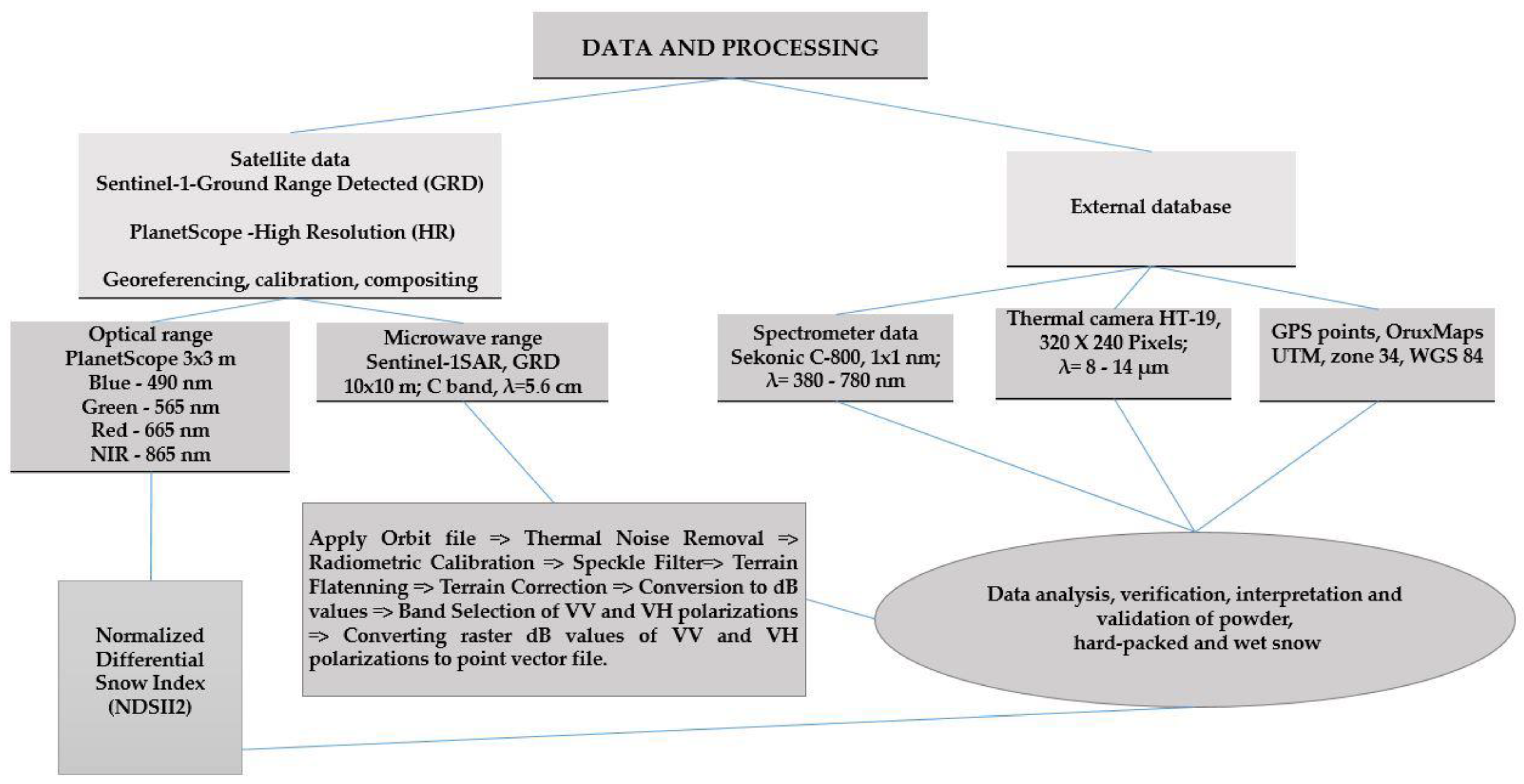
2.2. Data and Processing of Various Data Types
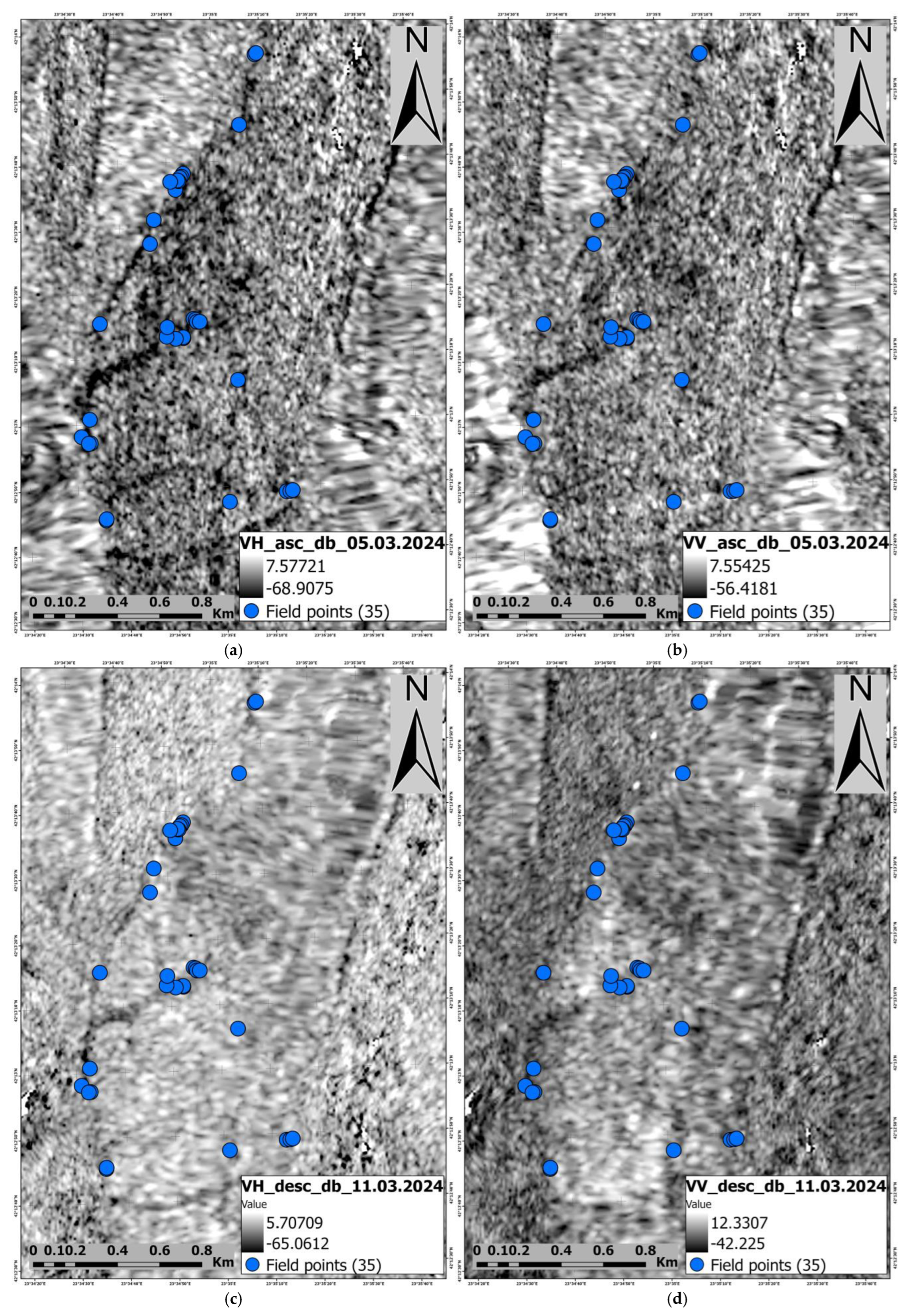
2.2.1. SAR Data
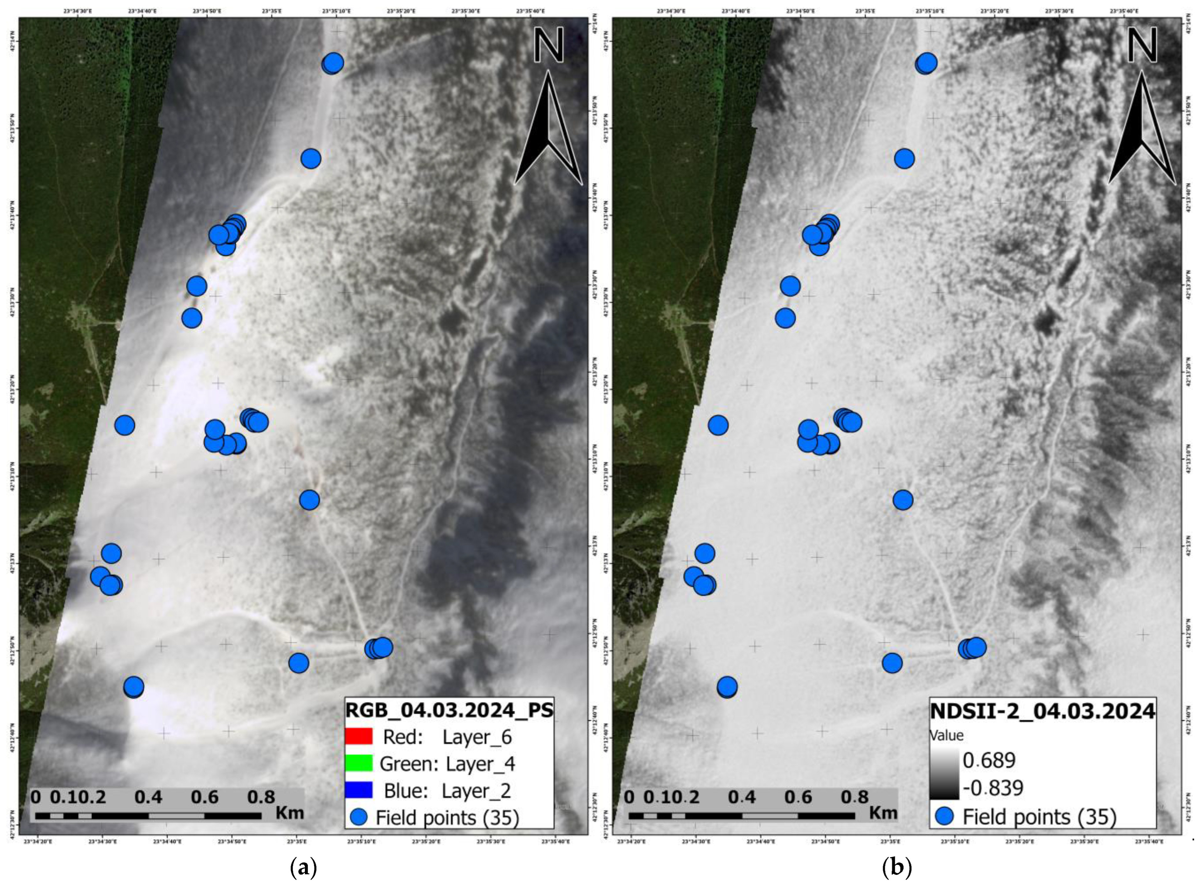
2.2.2. High-Resolution Data from PlanetScope
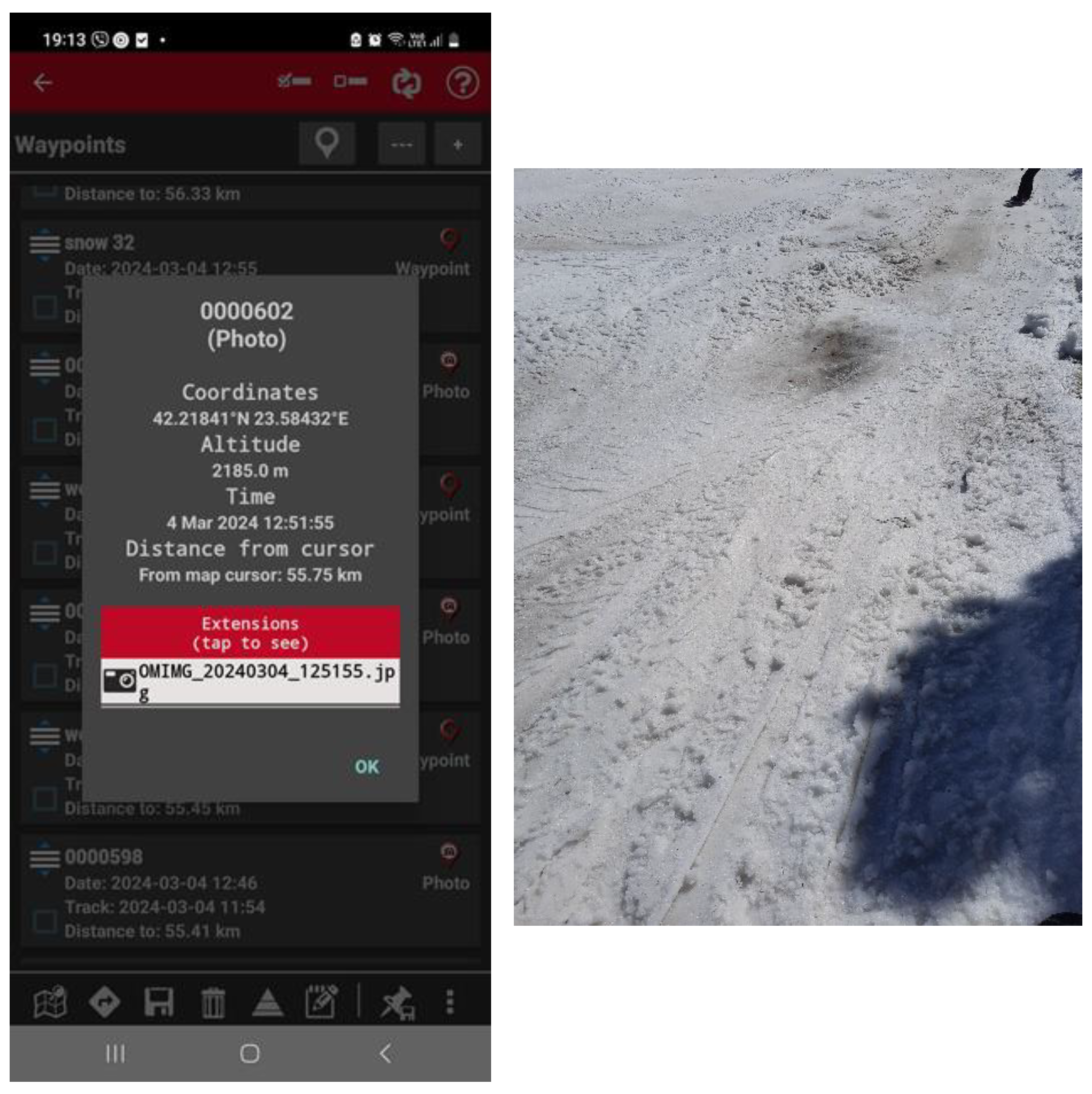
2.2.3. Field (In Situ) Data
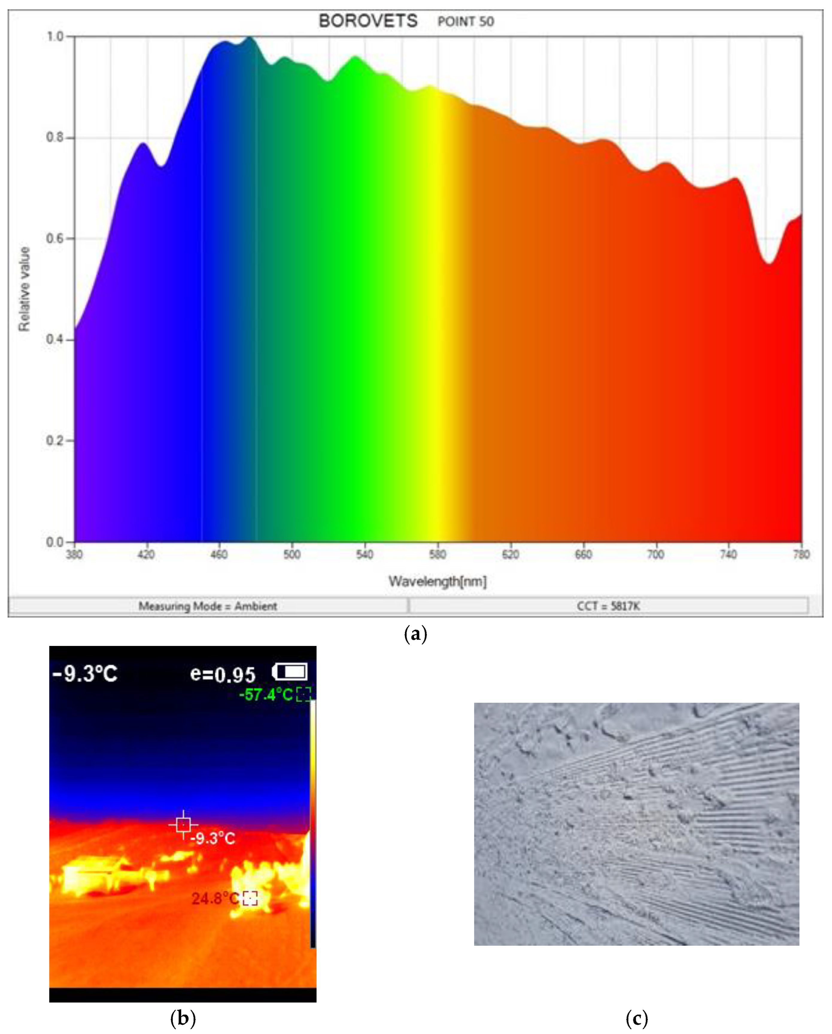
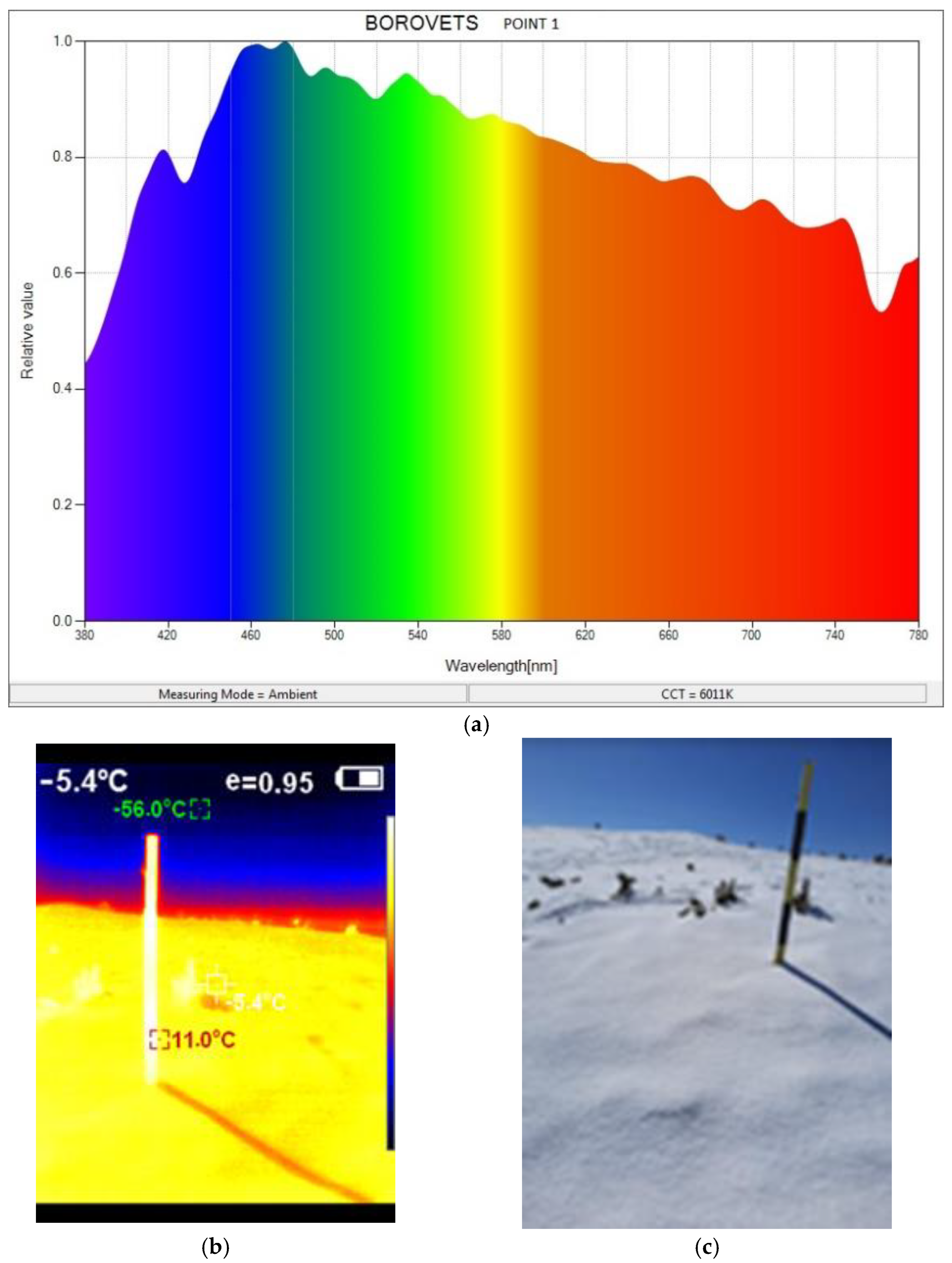
Mobile Spectrometer
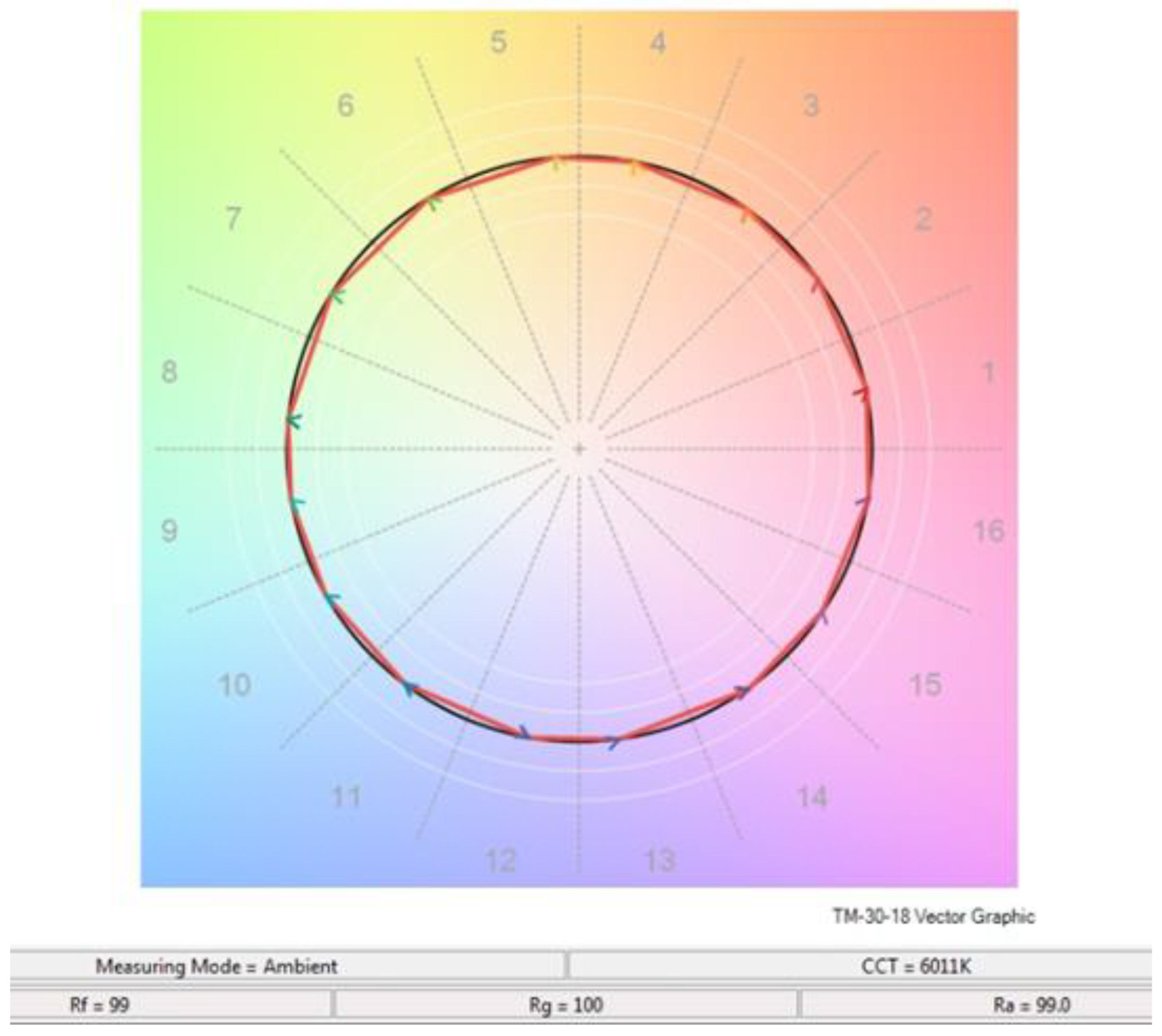
Color Vector Graph
Mobile Thermal Camera
2.3. Methods
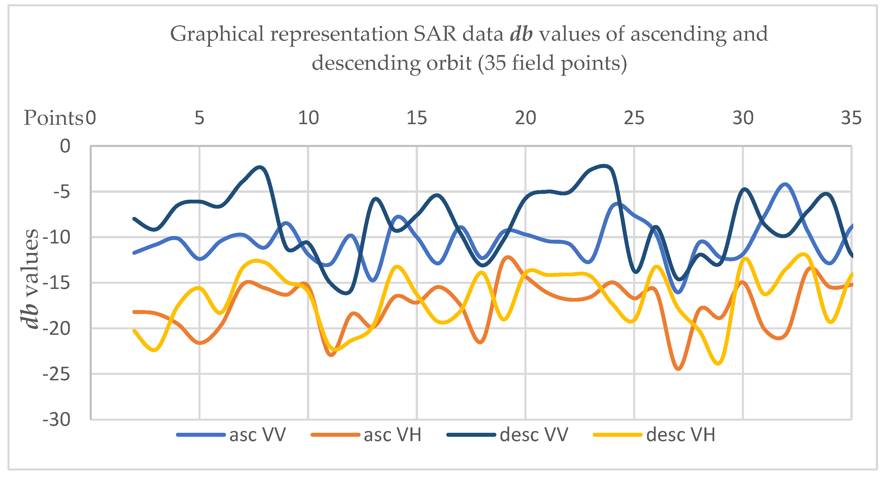
2.3.1. Remote Sensing Methods for Analysis of Powder, Hard-Packed, and Wet Snow Monitoring Based on SAR Data
2.3.2. Remote Sensing Methods and Indices for Analysis of Powder, Hard-Packed, and Wet Snow Based on Optical Data
Normalized Difference Snow Index (NDSI)
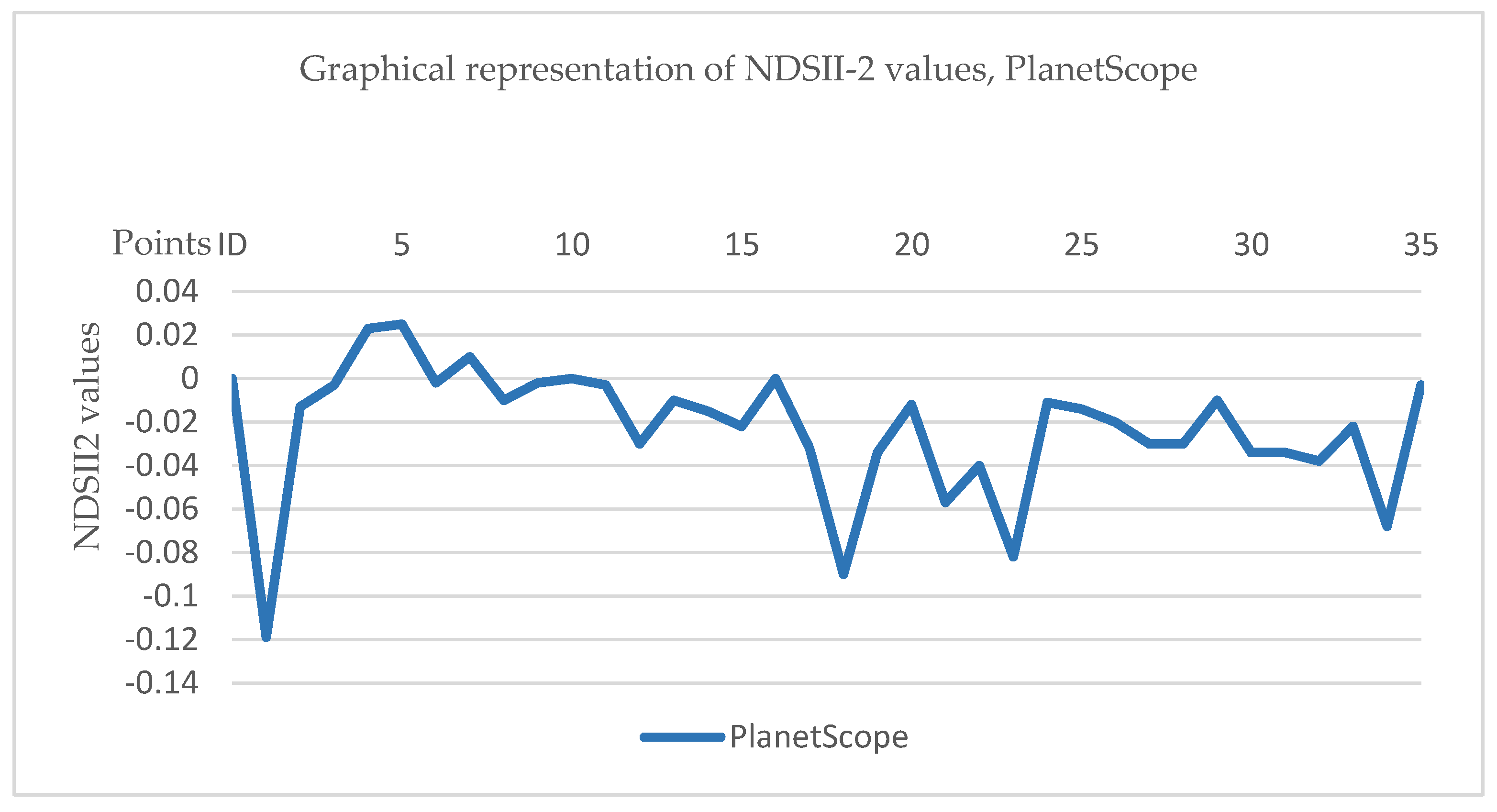
Normalized Difference Snow Ice Index-2 (NDSII2)
2.3.3. Verification
3. Results
3.1. Test Site
3.2. Validation Using In Situ Data
4. Discussion
5. Conclusions
Author Contributions
Funding
Data Availability Statement
Conflicts of Interest
Appendix A

| Spectral Parameters | Value Point 1 Powder Snow | Value Point 5 Powder Snow | Value Point 46 Wet Snow | Value Point 50 Hard-Packed | Value Point 61 Hard-Packed |
|---|---|---|---|---|---|
| CCT [K] | 6011 | 6137 | 5794 | 5817 | 6099 |
| CRI, Ra | 99 | 98.9 | 99.4 | 99.2 | 99.0 |
| CRI R1 | 98.7 | 98.5 | 99.5 | 99.0 | 98.7 |
| CRI R2 | 98.9 | 98.8 | 99.3 | 99.0 | 98.9 |
| CRI R3 | 99.6 | 99.7 | 99.5 | 99.5 | 99.7 |
| CRI R4 | 98.8 | 98.6 | 99.5 | 98.9 | 98.7 |
| CRI R5 | 98.6 | 98.5 | 99.4 | 98.8 | 98.6 |
| CRI R6 | 98.7 | 98.6 | 99.2 | 99.5 | 98.7 |
| CRI R7 | 99.7 | 99.8 | 99.4 | 99.8 | 99.8 |
| CRI R8 | 99.3 | 99.0 | 99.5 | 99.1 | 99.2 |
| CRI R9 | 97.4 | 96.6 | 99.0 | 99.0 | 97.2 |
| CRI R10 | 97.9 | 97.8 | 98.8 | 98.2 | 97.9 |
| CRI R11 | 98.4 | 98.2 | 99.3 | 98.7 | 98.3 |
| CRI R12 | 97.1 | 97.0 | 97.9 | 97.2 | 97.1 |
| CRI R13 | 98.6 | 98.4 | 99.2 | 98.8 | 98.5 |
| CRI R14 | 99.8 | 99.8 | 99.8 | 99.7 | 99.8 |
| CRI R15 | 98.6 | 98.3 | 99.5 | 99.0 | 98.5 |
| CIE1931 x | 0.3220 | 0.3194 | 0.3260 | 0.3255 | 0.3201 |
| CIE1931 y | 0.3335 | 0.3319 | 0.3389 | 0.3379 | 0.3327 |
| Hue | 29 deg | 28 deg | 39 deg | 37 deg | 30 deg |
| Saturation | 5% | 4% | 9% | 9% | 4% |
| TM 30-18 | Rf = 99 | Rf = 99 | Rf = 99 | Rf = 99 | Rf = 99 |
| TM 30-18 | Rg = 100 | Rg = 101 | Rg = 100 | Rg = 100 | Rg = 101 |
| TM 30-18 | Ra = 99.0 | Ra = 98.9 | Ra = 99.4 | Ra = 99.2 | Ra = 99.0 |


References
- Viviroli, D.; Weingartner, R. The hydrological significance of mountains: From regional to global scale. Hydrol. Earth Syst. Sci. 2004, 8, 1017–1030. [Google Scholar] [CrossRef]
- Fernandes, R.A.; Zhou, F.; Song, H. Evaluation of Multiple Datasets for Producing Snow-Cover Indicators for Canada; Geomatics Canada: Ottawa, ON, Canada, 2017. [Google Scholar]
- Dixit, A.; Goswami, A.; Jain, S. Development and Evaluation of a New “Snow Water Index (SWI)” for Accurate Snow Cover Delineation. Remote Sens. 2019, 11, 2774. [Google Scholar] [CrossRef]
- Gupta, R.P.; Haritashya, U.K.; Singh, P. Mapping dry/wet snow cover in the Indian Himalayas using IRS multispectral im-agery. Remote Sens. Environ. 2005, 97, 458–469. [Google Scholar] [CrossRef]
- Shimamura, Y.; Izumi, T.; Matsumaya, H. Evaluation of a useful method to identify snow-covered areas under vegetation–comparisons among a newly proposed snow index, normalized di erence snow index and visible reflectance. Int. J. Remote Sens. 2006, 27, 4867–4884. [Google Scholar] [CrossRef]
- Sibandze, P.; Mhangara, P.; Odindi, J.; Kganyago, M. A comparison of Normalised Di erence Snow Index (NDSI) and Nor-malised Di erence Principal Component Snow Index (NDPCSI) techniques in distinguishing snow from related land cover types. S. Afr. J. Geomat. 2014, 3, 197–209. [Google Scholar] [CrossRef]
- Valovcin, F.R. Snow/Cloud Discrimination; AFGL-TR-76-0174, ADA 032385; Air Force Geophysics Laboratory Hanscom AFB Mass: Bedford, MA, USA, 1976. [Google Scholar]
- Valovcin, F.R. Spectral Radiance of Snow and Clouds in the Near Infrared Spectral Region; AFGL-TR-78-0289, ADA 063761; Air Force Geophysics Laboratory Hanscom AFB Mass: Bedford, MA, USA, 1978. [Google Scholar]
- Kyle, H.L.; Curran, R.J.; Barnes, W.L.; Escoe, D. A cloud Physics Radiometer. In Proceedings of the Third Conference on Atmospheric Radiation, American Meteorological Society, Davis, CA, USA, 28–30 June 1978; p. 107. [Google Scholar]
- Rees, W.G. Remote Sensing of Snow and Ice; CRC Press: Boca Raton, FL, USA, 2006; pp. 137–156. [Google Scholar]
- Thakur, P.K.; Garg, R.D.; Aggarwal, S.P.; Garg, P.K.; Shi, J. Snow density retrieval using SAR data: Algorithm validation and applications in part of North Western Himalaya. Cryosphere Discuss. 2013, 7, 1927–1960. [Google Scholar] [CrossRef]
- Rango, A.; Salomonson, V.V.; Foster, J.L. Employment of satellite snow cover observations for Improving Seasonal Runoff Estimates. In Operational Applications of Satellite Snow Cover Observations; NASA-SP-391; NASA: Washington, DC, USA, 1975; pp. 157–174. [Google Scholar]
- Dhanju, M.S. Studies of Himalayan snow cover area from satellites. Hydrological Applications of Remote Sensing and Remote Data Transmission. In Proceedings of the Hamburg Symposium, IAHS, Hamburg, Germany, 15–26 August 1983; Volume 145, pp. 401–409. [Google Scholar]
- Dozier, J. Snow reflectance from Landsat-4 Thematic Mapper. IEEE Trans. Geosci. Remote Sens. 1984, 22, 323–328. [Google Scholar] [CrossRef]
- Dozier, J. Spectral signature of Alpine snow cover from the Landsat Thematic Mapper. Remote Sens. Environ. 1989, 28, 9–22. [Google Scholar] [CrossRef]
- Hall, D.K.; Riggs, G.A.; Salomonson, V.V. Development of methods for mapping global snow cover using moderate resolution imaging spectroradiometer data. Remote Sens. Environ. 1995, 54, 127–140. [Google Scholar] [CrossRef]
- Dozier, J. Remote Sensing of the Alpine Snow Cover: A Review of Techniques and Accomplishments from the Visible Wavelengths Through the Microwave. In Proceedings of the International Conference on Snow 5 Hydrology the Integration of Physical, Chemical, and Biological Systems, Brownsville, VT, USA, 6–9 October 1998; 03755-1290, Special Report. US Army Cold Regions Research and Engineering Laboratory Hanover: New Hampshire, NH, USA, 1998; pp. 98–110. [Google Scholar]
- Dozier, J.; Painter, H.T. Multispectral and hyperspectral remote sensing of alpine snow properties. Annu. Rev. Earth Planet. Sci. 2004, 32, 465–494. [Google Scholar] [CrossRef]
- Braun, M.; Rau, F. Using a multi-year data archive of ERS-SAR imagery for monitoring snow line positions and ablation patters on the King George Island ice cap (Antarctica). EARSeL eProc. 2001, 1, 281–291. [Google Scholar]
- Rau, F.; Braun, M.; Friedrich, M.; Weber, F.; Gobmann, H. Radar glacier zones and its boundaries as indicators of glacier mass balance and climatic variability. EARSeL eProc. 2001, 1, 317–327. [Google Scholar]
- Storvold, R.; Malnes, E.; Larsen, Y.; Høgda, K.A.; Hamran, S.E.; Muller, K.; Langley, K.A. SAR Remote Sensing of Snow Parameters in Norwegian Areas—Current Status and Future Perspective. In Proceedings of the Progress in Electromagnetics Research Symposium, Cambridge, MA, USA, 26–29 March 2006; pp. 182–186. [Google Scholar]
- Thakur, P.K.; Snehmani, P.V.H.; Aggarwal, S.P.; Jain, S.K. Snow Cover Mapping Using Multi-Sensor SAR Data for Parts of Western Himalayas. In Proceedings of the International Symposium on Snow and Avalanches (ISSA), at Snow and Avalanche Establishment (SASE), Manali, India, 6–10 April 2009. [Google Scholar]
- Venkataraman, G.; Singh, G.; Kumar, V. Snow Cover Area Monitoring Using Multitemporal TerraSARX Data. In Proceedings of the Third TerraSAR-X Science Team Meeting, DLR, Hamburg, Germany, 25–26 November 2008. [Google Scholar]
- Wang, L.; Toose, P.; Brown, R.; Derksen, C. Frequency and distribution of winter melt events from passive microwave satellite data in the pan-Arctic, 1988–2013. Cryosphere 2016, 10, 2589–2602. [Google Scholar] [CrossRef]
- Grenfell, T.C.; Putkonen, J. A method for the detection of the severe rain-on-snow event on Banks Island, October 2003, using passive microwave remote sensing. Water Resour. Res. 2008, 44, 1–9. [Google Scholar] [CrossRef]
- Dolant, C.; Langlois, A.; Montpetit, B.; Brucker, L.; Roy, A.; Royer, A. Development of a rain-on-snow detection algorithm using passive microwave radiometry. Hydrol. Process. 2016, 30, 3184–3196. [Google Scholar] [CrossRef]
- Langlois, A.; Johnson, C.A.; Montpetit, B.; Royer, A.; Blukacz-Richards, E.A.; Neave, E.; Dolant, C.; Roy, A.; Arhonditsis, G.; Kim, D.K.; et al. Detection of rain-on-snow (ROS) events and ice layer formation using passive microwave radiometry: A context for Peary caribou habitat in the Canadian Arctic. Remote Sens. Environ. 2017, 189, 84–95. [Google Scholar] [CrossRef]
- Pan, C.G.; Kirchner, P.B.; Kimball, J.S.; Kim, Y.; Du, J. Rain-on-snow events in Alaska, their frequency and distribution from satellite observations. Environ. Res. Lett. 2018, 13, 075004. [Google Scholar] [CrossRef]
- Kunzi, K.; Patil, S.; Rott, H. Snow-Cover Parameters Retrieved from Nimbus-7 Scanning Multichannel Microwave Radiometer (SMMR) Data. IEEE Trans. Geosci. Remote Sens. 1982, GE-20, 452–467. [Google Scholar] [CrossRef]
- WMO. Review on Remote Sensing of the Snow Cover and on Methods of Mapping Snow; World Meteorological Organization: Geneva, Switzerland, 2012. [Google Scholar]
- Singh, G.; Yamaguchi, Y.; Park, S.E.; Venkataraman, G. Identification of Snow using SAR Polarimetry techniques. Int. Arch. Photogramm. Remote Sens. Spat. Inf. Sci. 2010, 38 Pt 8, 146–149. [Google Scholar]
- Martini, A. Télédétection d’un Couvert Neigeux en Milieux Alpins à Partir de Données SAR Polarimétriques Multi-Fréquentielles et Multitemporelles. Ph.D. Thesis, Universite de Rennes, Rennes, France, 2005. [Google Scholar]
- Magagi, R.; Bernier, M. Optimal conditions for wet snow detection using RADARSAT SAR data. Remote Sens. Environ. 2003, 84, 221–233. [Google Scholar] [CrossRef]
- Marin, C.; Bertoldi, G.; Premier, V.; Callegari, M.; Brida, C.; Hürkamp, K.; Tschiersch, J.; Zebisch, M.; Notarnicola, C. Use of Sentinel-1 radar observations to evaluate snowmelt dynamics in alpine regions. Cryosphere 2020, 14, 935–956. [Google Scholar] [CrossRef]
- Nagler, T.; Rott, H. Retrieval of wet snow by means of multitemporal SAR data. IEEE Trans. Geosci. Remote Sens. 2000, 38, 754–765. [Google Scholar] [CrossRef]
- Rott, H.; Mätzler, C. Possibilities and limits of synthetic aperture radar for snow and glacier surveying. Ann. Glaciol. 1987, 9, 195–199. [Google Scholar] [CrossRef]
- Antropova, Y.K.; Komarov, A.S.; Richardson, M.; Millard, K.; Smith, K. Detection of wet snow in the Arctic tundra from time-series fully-polarimetric RADARSAT-2 images. Remote Sens. Environ. 2022, 283, 113305. [Google Scholar] [CrossRef]
- Donahue, C.; Hammonds, K. Laboratory Observations of Preferential Flow Paths in Snow Using Upward-Looking Polari-metric Radar and Hyperspectral Imaging. Remote Sens. 2022, 14, 2297. [Google Scholar] [CrossRef]
- Nagler, T.; Rott, H.; Ripper, E.; Bippus, G.; Hetzenecker, M. Advancements for Snowmelt Monitoring by Means of Sentinel-1 SAR. Remote Sens. 2016, 8, 348. [Google Scholar] [CrossRef]
- Idowu, A.N.; Marshall, H.-P. Snow Depth Retrieval from L-Band Data Based on Repeat Pass InSAR Techniques. In Proceedings of the IGARSS 2022—2022 IEEE International Geoscience and Remote Sensing Symposium, Kuala Lumpur, Malaysia, 17–22 July 2022; pp. 4248–4251. [Google Scholar] [CrossRef]
- Snehmani; Venkataraman, G.; Nigam, A.K.; Singh, G. Development of an inversion algorithm for dry snow density estimation and its application with ENVISAT-ASAR dual co-polarization data. Geocarto Int. 2010, 25, 597–616. [Google Scholar] [CrossRef]
- Kay, J.E.; Gillespie, A.R.; Hansen, G.B.; Pettit, E.C. Spatial relationships between snow contaminant content, grain size, and surface temperature from multispectral images of Mt. Rainier, Washington (USA). Remote Sens. Environ. 2003, 86, 216–231. [Google Scholar] [CrossRef]
- Tonooka, H.; Watanabe, A. Applicability of Thermal Infrared Surface Emissivity Ratio for Snow/Ice Monitoring. In SPIE 5655, Multispectral and Hyperspectral Remote Sensing Instruments and Applications II, Proceedings of the Fourth International Asia-Pacific Environmental Remote Sensing Symposium 2004: Remote Sensing of the Atmosphere, Ocean, Environment, and Space, Honolulu, Hawaii, USA, 8–12 November 2004; Larar, A.M., Suzuki, M., Tong, Q., Eds.; Society of Photo Optical: Bellingham, WA, USA, 2005. [Google Scholar] [CrossRef]
- Hori, M.; Aoki, T.; Tanikawa, T.; Motoyoshi, H.; Hachikubo, A.; Sugiura, K.; Yasunari, T.J.; Eide, H.; Storvold, R.; Nakajima, Y.; et al. In-situ measured spectral directional emissivity of snow and ice in the 8–14 μm atmospheric window. Remote Sens. Environ. 2006, 100, 486–502. [Google Scholar] [CrossRef]
- Hori, M.; Aoki, T.; Tanikawa, T.; Kuchiki, K.; Niwano, M.; Yamaguchi, S.; Matoba, S. Dependence of Thermal Infrared Emissive Behaviors of Snow Cover on the Surface Snow Type. Bull. Glaciol. Res. 2014, 320, 33. [Google Scholar] [CrossRef]
- Mishev, D. Remote Earth Exploration from Space; Bulgarian Academy of Sciences Publishing House: Sofia, Bulgaria, 1981; p. 206. [Google Scholar]
- Available online: https://www.oruxmaps.com/cs/en/ (accessed on 27 April 2025).
- Software Guide of “C-800 Utility” for C-800 SPECTROMETER. Available online: https://global.sekonic.com/downloads/?product=401-800 (accessed on 27 April 2025).
- Ht-19 Thermal Camera Manual. Available online: https://hti-instrument.com/pages/ht-19-manual (accessed on 27 April 2025).
- Available online: https://bg.benweilighting.com/info/cct-understanding-correlated-color-temperatur-84542133.html (accessed on 27 April 2025).
- Available online: https://www.meteoswiss.admin.ch/weather/weather-and-climate-from-a-to-z/snow/types-of-snow.html (accessed on 27 April 2025).
- Available online: https://compuweather.com/the-important-difference-between-wet-snow-and-dry-snow/ (accessed on 27 April 2025).
- Available online: https://www.acurite.com/blogs/weather-101/types-of-snow?srsltid=AfmBOoowqd602gFqNOlIskJSchC5jnfhAd7LRCCtBn0Iw_6elXYd1gG9 (accessed on 27 April 2025).
- Assenov, A. Biogeography and Natural Capital of Bulgaria; University Press St. Kliment Ohridski: Sofia, Bulgaria, 2021. (In Bulgarian) [Google Scholar]
- Available online: http://www.journey.bg/bulgaria/bulgaria.php?guide=4338 (accessed on 27 April 2025).
- Available online: https://sentinel.esa.int/web/sentinel/missions/sentinel-1 (accessed on 27 April 2025).
- Karbou, F.; Veyssière, G.; Coleou, C.; Dufour, A.; Gouttevin, I.; Durand, P.; Gascoin, S.; Grizonnet, M. Monitoring Wet Snow Over an Alpine Region Using Sentinel-1 Observations. Remote Sens. 2021, 13, 381. [Google Scholar] [CrossRef]
- Kropatsch, W.G.; Strobl, D. The generation of SAR layover and shadow maps from digital elevation models. IEEE Trans. Geosci. Remote Sens. 1990, 28, 98–107. [Google Scholar] [CrossRef]
- Gelautz, M.; Frick, H.; Raggam, J.; Burgstaller, J.; Leberl, F. SAR image simulation and analysis of alpine terrain. ISPRS J. Photogramm. Remote Sens. 1998, 53, 17–38. [Google Scholar] [CrossRef]
- Lillesand, T.M.; Kiefer, R.W. Remote Sensing and Photo Interpretation; John Wiley and Sons: New York, NY, USA, 1994; p. 750. [Google Scholar]
- Available online: https://step.esa.int/main/download/snap-download (accessed on 27 April 2025).
- Available online: https://step.esa.int/main/doc/tutorials/ (accessed on 27 April 2025).
- Available online: https://step.esa.int/main/toolboxes/snap/ (accessed on 27 April 2025).
- Available online: https://browser.stac.dataspace.copernicus.eu/collections/sentinel-1-grd?.language=en (accessed on 27 April 2025).
- Pan, B.; Shi, X. Fusing Ascending and Descending Time-Series SAR Images with Dual-Polarized Pixel Attention UNet for Landslide Recognition. Remote Sens. 2023, 15, 5619. [Google Scholar] [CrossRef]
- Available online: https://www.esri.com/en-us/arcgis/products/arcgis-pro/overview (accessed on 27 April 2025).
- Available online: https://developers.planet.com/docs/data/planetscope/ (accessed on 27 April 2025).
- Spasova, T.; Avetisyan, D. Remote Sensing in Polar Regions Antarctic Part I, for Space Research and Technology Institute; Bulgarian Academy of Sciences: Sofia, Bulgaria, 2024; ISBN 978-619-7490-19-0. 978-619-7490-14-5. [Google Scholar]
- Available online: https://bgledfactory.bg/blog-article/44/kakvo-e-indeks-na-tsvetopredavane-cri.html (accessed on 27 April 2025).
- Available online: https://lightingequipmentsales.com/cct-kelvin.html (accessed on 27 April 2025).
- Available online: https://bg.benweilight.com/info/what-is-cct-how-to-choose-cct-for-led-lightin-69257544.html (accessed on 27 April 2025).
- Available online: https://learn.leighcotnoir.com/artspeak/elements-color/hue-value-saturation (accessed on 27 April 2025).
- Available online: https://en.wikipedia.org/wiki/Hue (accessed on 27 April 2025).
- Available online: https://www.uprtek.com/en/blogs/what-is-tm-30-15-tm-30-18-and-should-i-use-it (accessed on 27 April 2025).
- Available online: https://luminusdevices.zendesk.com/hc/en-us/articles/4421188803469-What-are-the-TM-30-18-Color-Rendition-Guidelines-Reports (accessed on 27 April 2025).
- Spasova, T.; Avetisyan, D.; Stoyanov, A. Snow Cover Mapping Based on a Multi-Index Technique in Vitosha, Pirin and Rila mountains. In Proceedings of the SPIE 13197, Earth Resources and Environmental Remote Sensing/GIS Applications XV, 131971B, Edinburgh, UK, 16–20 September 2024. [Google Scholar] [CrossRef]
- Available online: https://global.sekonic.com/sekonic-c-800-spectrometer/ (accessed on 27 April 2025).
- Mätzler, C. Applications of the interaction of microwaves with the natural snow cover. Remote Sens. Rev. 1987, 2, 259–387. [Google Scholar] [CrossRef]
- Rignot, E.; Echelmeyer, K.; Krabill, W. Penetration depth of interferometric synthetic-aperture radar signals in snow and ice. Geophys. Res. Lett. 2001, 28, 3501–3504. [Google Scholar] [CrossRef]
- Langley, K.; Hamran, S.-E.; Hogda, K.A.; Storvold, R.; Brandt, O.; Hagen, J.O.; Kohler, J. Use of C-Band Ground Penetrating Radar to Determine Backscatter Sources Within Glaciers. IEEE Trans. Geosci. Remote Sens. 2007, 45, 1236–1246. [Google Scholar] [CrossRef]
- Shi, J.; Dozier, J. Inferring snow wetness using C-band data from SIR-C’s polarimetric synthetic aperture radar. IEEE Trans. Geosci. Remote Sens. 1995, 33, 905–914. [Google Scholar]
- Mätzler, C.; Schanda, E. Snow mapping with active microwave sensors. Int. J. Remote Sens. 1984, 5, 409–422. [Google Scholar] [CrossRef]
- Spasova, T. Polar digital space in Antarctica. In Proceedings SPIE 12728, Proceedings of the Remote Sensing of the Ocean, Sea Ice, Coastal Waters, and Large Water Regions 2023, 127280P, Amsterdam, The Netherlands, 3–6 September 2023; Bostater Jr., C.R., Neyt, X., Eds.; SPIE: Bellingham, WA, USA, 2023. [Google Scholar] [CrossRef]
- Jiskoot, H. Glacier Surging. In Encyclopedia of Snow, Ice and Glaciers; Singh, V.P., Singh, P., Haritashya, U.K., Eds.; Springer: Dordrecht, The Netherlands, 2011; pp. 415–428. ISBN 978-9-04-812641-5. [Google Scholar]
- Teleubay, Z.; Yermekov, F.; Tokbergenov, I.; Toleubekova, Z.; Igilmanov, A.; Yermekova, Z.; Assylkhanova, A. Comparison of Snow Indices in Assessing Snow Cover Depth in Northern Kazakhstan. Sustainability 2022, 14, 9643. [Google Scholar] [CrossRef]
- Available online: https://hexagon.com/products/erdas-imagine (accessed on 27 April 2025).
- Mardirosyan, G. Natural Disasters and Ecological Catastrophes; Bulgarian Academy of Sciences Publishing House: Sofia, Bulgaria, 2009. [Google Scholar]
- Mardirosyan, G. Fundamentals of Remote Aerospace Technologies; New Bulgarian University: Sofia, Bulgaria, 2015; p. 238. ISBN 978-954-535-882-1. [Google Scholar]
- Spasova, T.; Avetisyan, D. A Synchronized Remote Sensing Monitoring Approach in the Livingstone is-Land Region of Antarctica, In Proceedings SPIE 12786, Proceedings of the Ninth International Conference on Remote Sensing and Geoinformation of the Environment (RSCy2023), 127861X, Ayia Napa, Cyprus, 3–5 April 2023; Themistocleous, K., Hadjimitsis, D.G., Michaelides, S., Papadavid., G., Eds.; SPIE: Bellingham, WA, USA, 2023. [Google Scholar]
- Borisova, D.; Hristova, V.; Dimitrov, V.M. Thematic Spectral Library for Remote Sensing Monitoring of Land Covers in Local Scale. In Proceedings SPIE 11534, Proceedings of the Earth Resources and Environmental Remote Sensing/GIS Applications XI, 1153408 20–21 September 2020; Schulz, K., Ed.; SPIE: Bellingham, WA, USA, 2020. [Google Scholar] [CrossRef]
- Ohno, Y. CIE fundamentals for Color Measurements. In Proceedings of the Paper for IS&T NIP16 Conference, Vancouver, BC, Canada, 16–20 October 2000; pp. 540–545. [Google Scholar]
- Borisova, D.; Kancheva, R.; Nikolov, H. Spectral Mixture Analysis of Land Covers. In Proceedings of the 25th EARSeL Symposium, Porto, Portugal, 6–11 June 2005; Global Developments in Environmental Earth Observation from Space. Millpress: Roterdam, The Netherlands, 2006; pp. 509–516. [Google Scholar]
- Mishev, D. Spectral Characteristics of Natural Objects; Bulgarian Academy of Sciences Publishing House: Sofia, Bulgaria, 1986; p. 192. [Google Scholar]
- Atanassov, V.; Jelev, G.; Kraleva, L. Imaging Spectrometer Data Correction. In Proceedings of the Scientific Conference with International Participation “Space, Ecology, Safety—SES’2005” Conference Proceedings, Book 1, Varna, Bulgaria, 10–13 June 2005; pp. 221–226. [Google Scholar]
- Spasova, T. Creating a Digital Twin and Polar Digital space in Antarctica. In Proceedings SPIE 12786, Ninth International Conference on Remote Sensing and Geoinformation of the Environment (RSCy2023), 12786, Ayia Napa, Cyprus, 3–5 April 2023; SPIE: Bellingham, WA, USA, 2023; ISSN 0277786X. [Google Scholar] [CrossRef]
- Ulaby, F.T.; Long, D.G.; Press, M. Microwave Radar and Radiometric Remote Sensing; Ulaby, F.T., Ed.; The University of Michigan Press: Ann Arbor, MI, USA, 2014. [Google Scholar]
- Dasser, G.; Bickel, V.T.; Rüetschi, M.; Jacquemart, M.; Bavay, M.; Hafner, E.D.; van Herwijnen, A.; Manconi, A. Moni-Toring Snow Wetness Evolution from Satellite with Sentinel-1 Multi-Track Composites, EGUsphere 2024. Available online: https://egusphere.copernicus.org/preprints/2024/egusphere-2024-1510/ (accessed on 27 April 2025).
- Beltramone, G.; Frery, A.C.; Rotela, C.; Germán, A.; Bonansea, M.; Scavuzzo, C.M.; Ferral, A. Identification of Seasonal Snow Phase Changes from C-Band SAR Time Series with Dynamic Thresh-olds. IEEE J. Sel. Top. Appl. Earth Obs. Remote Sens. 2023, 16, 6995–7008. [Google Scholar] [CrossRef]
- Spasova, T.; Nedkov, R. Monitoring of Short-Lived Snow Coverage by Radar and Optical Data from Sentinel-1 and Sentinel-2 Satellites. Ecol. Eng. Environ. Prot. 2017, 2, 13–19. [Google Scholar] [CrossRef]
- Spasova, T.; Dancheva, A.; Avetisyan, D.; Ivanova, I.; Popov, I.; Shirov, B. Monitoring of renewable energy sources with remote sensing, open data, and field data in Bulgaria. In Proceedings of the SPIE 12733, Image and Signal Processing for Remote Sensing XXIX, 1273311, Amsterdam, The Netherlands, 4–5 September 2023; SPIE: Bellingham, WA, USA, 2023. [Google Scholar] [CrossRef]


| Satellite | Date | Spectral Band, Wavelength | Spatial Resolution |
|---|---|---|---|
| Sentinel-1-A | 5 March 2024 11 March 2024 | λ = 5.6 ϲm, C band Polarization: VH, VV | 10 × 10 m |
| PlanetScope | 4 March 2024 | Coastal Blue—443 nm Blue—490 nm Green I—531 nm Green—565 nm Yellow—610 nm Red—665 nm Red edge—705 nm NIR—865 nm | 3 × 3 m |
| Sekonic C-800 mobile spectrometer | 4 March 2024 | 380 to 780 nm | 1 nm |
| HT-19 thermal camera | 4 March 2024 | 8 to 14 μm | 320 × 240 Pixels |
| ID | Points | Snow Type | Asc VV | Asc VH | Desc VV | Desc VH | PlanetScope PSB.SD NDSII2 | Color Temperature (CCT), [K] |
|---|---|---|---|---|---|---|---|---|
| 1 | 3 | Wet snow | −11.72 | −18.2 | −7.99 | −20.27 | −0.119 | 5794 |
| 2 | 4 | Wet snow | −10.81 | −18.37 | −9.14 | −22.33 | −0.013 | 5837 |
| 3 | 44 | Wet snow | −10.14 | −19.52 | −6.5 | −17.56 | −0.003 | 5770 |
| 4 | 45 | Wet snow | −12.39 | −21.6 | −6.1 | −15.59 | 0.023 | 5790 |
| 5 | 46 | Wet snow | −10.4 | −19.64 | −6.57 | −18.27 | 0.025 | 5794 |
| 6 | 15 | Hard-packed | −9.74 | −15.15 | −3.86 | −13.34 | −0.002 | 5990 |
| 7 | 16 | Hard-packed | −11.14 | −15.58 | −2.7 | −12.76 | 0.010 | 5990 |
| 8 | 24 | Hard-packed | −8.46 | −16.31 | −11.16 | −14.88 | −0.010 | 5910 |
| 9 | 25 | Hard-packed | −11.88 | −15.38 | −10.64 | −15.97 | −0.002 | 5839 |
| 10 | 27 | Hard-packed | −12.98 | −22.89 | −14.97 | −22.01 | 0.000 | 5839 |
| 11 | 28 | Hard-packed | −9.83 | −18.43 | −15.71 | −21.31 | −0.003 | 5839 |
| 12 | 39 | Hard-packed | −14.73 | −19.84 | −5.97 | −19.69 | −0.030 | 6282 |
| 13 | 50 | Hard-packed | −7.93 | −16.51 | −9.27 | −13.32 | −0.010 | 5817 |
| 14 | 58 | Hard-packed | −9.99 | −17.17 | −7.6 | −16.27 | −0.015 | 6099 |
| 15 | 61 | Hard-packed | −12.87 | −15.46 | −5.44 | −19.29 | −0.022 | 6099 |
| 16 | 1 | Powder snow | −8.9 | −17.42 | −9.54 | −18.12 | −0,029 | 6011 |
| 17 | 5 | Powder snow | −12.29 | −21.41 | −13.09 | −13.89 | −0.032 | 6137 |
| 18 | 6 | Powder snow | −9.38 | −12.52 | −10.27 | −19.03 | −0.09 | 5928 |
| 19 | 8 | Powder snow | −9.7 | −14.31 | −5.75 | −13.93 | −0.034 | 5928 |
| 20 | 9 | Powder snow | −10.42 | −16.09 | −5 | −14.14 | −0.012 | 5847 |
| 21 | 10 | Powder snow | −10.72 | −16.84 | −5.07 | −14.09 | −0.057 | 5820 |
| 22 | 14 | Powder snow | −12.61 | −16.54 | −2.61 | −14.29 | −0.040 | 6177 |
| 23 | 17 | Powder snow | −6.6 | −14.95 | −2.78 | −17.32 | −0.082 | 5841 |
| 24 | 29 | Powder snow | −7.61 | −16.71 | −13.7 | −19.1 | −0.011 | 5933 |
| 25 | 30 | Powder snow | −9.61 | −15.9 | −8.87 | −13.24 | −0.014 | 5933 |
| 26 | 31 | Powder snow | −16.05 | −24.44 | −14.57 | −17.71 | −0.020 | 6207 |
| 27 | 33 | Powder snow | −10.58 | −17.95 | −11.93 | −20.27 | −0.030 | 6137 |
| 28 | 38 | Powder snow | −12.24 | −18.8 | −12.75 | −23.59 | −0.030 | 6045 |
| 29 | 42 | Powder snow | −11.86 | −14.95 | −4.83 | −12.54 | −0.010 | 6001 |
| 30 | 47 | Powder snow | −7.64 | −20.11 | −8.62 | −16.26 | −0.034 | 6001 |
| 31 | 48 | Powder snow | −4.22 | −20.59 | −9.83 | −13.44 | −0.034 | 6001 |
| 32 | 52 | Powder snow | −9.41 | −13.55 | −7.11 | −12.18 | −0.038 | 6011 |
| 33 | 60 | Powder snow | −12.87 | −15.46 | −5.44 | −19.29 | −0.022 | 6120 |
| 34 | 63 | Powder snow | −8.92 | −15.22 | −11.88 | −14.21 | −0.068 | 6258 |
| 35 | 64 | Powder snow | −8.15 | −14.72 | −11.16 | −13.87 | −0.003 | 6258 |
| Asc VV | Wet Snow | Hard-Packed Snow | Powder Snow |
|---|---|---|---|
| min | – | – | V |
| max | – | – | V |
| asc VH | Wet snow | Hard-packed snow | Powder snow |
| min | – | – | V |
| max | – | – | V |
| Desc VV | Wet Snow | Hard-Packed Snow | Powder Snow |
|---|---|---|---|
| min | – | – | V |
| max | – | V | – |
| desc VH | Wet snow | Hard-packed snow | Powder snow |
| min | – | – | V |
| max | – | – | V |
Disclaimer/Publisher’s Note: The statements, opinions and data contained in all publications are solely those of the individual author(s) and contributor(s) and not of MDPI and/or the editor(s). MDPI and/or the editor(s) disclaim responsibility for any injury to people or property resulting from any ideas, methods, instructions or products referred to in the content. |
© 2025 by the authors. Licensee MDPI, Basel, Switzerland. This article is an open access article distributed under the terms and conditions of the Creative Commons Attribution (CC BY) license (https://creativecommons.org/licenses/by/4.0/).
Share and Cite
Stoyanov, A.; Spasova, T.; Avetisyan, D. An Analysis of Powder, Hard-Packed, and Wet Snow in High Mountain Areas Based on SAR, Optical Data, and In Situ Data. Remote Sens. 2025, 17, 1649. https://doi.org/10.3390/rs17091649
Stoyanov A, Spasova T, Avetisyan D. An Analysis of Powder, Hard-Packed, and Wet Snow in High Mountain Areas Based on SAR, Optical Data, and In Situ Data. Remote Sensing. 2025; 17(9):1649. https://doi.org/10.3390/rs17091649
Chicago/Turabian StyleStoyanov, Andrey, Temenuzhka Spasova, and Daniela Avetisyan. 2025. "An Analysis of Powder, Hard-Packed, and Wet Snow in High Mountain Areas Based on SAR, Optical Data, and In Situ Data" Remote Sensing 17, no. 9: 1649. https://doi.org/10.3390/rs17091649
APA StyleStoyanov, A., Spasova, T., & Avetisyan, D. (2025). An Analysis of Powder, Hard-Packed, and Wet Snow in High Mountain Areas Based on SAR, Optical Data, and In Situ Data. Remote Sensing, 17(9), 1649. https://doi.org/10.3390/rs17091649