Triple Graph Convolutional Network for Hyperspectral Image Feature Fusion and Classification

Abstract

Most graph-based networks utilize superpixel generation methods as a preprocessing step, considering superpixels as graph nodes. In the case of hyperspectral images having high variability in spectral features, considering an image region as a graph node may degrade the class discrimination ability of networks for pixel-based classification. Moreover, most graph-based networks focus on global feature extraction, while both local and global information are important for pixel-based classification. To deal with these challenges, superpixel-based graphs are overruled in this work, and a Graph-based Feature Fusion (GF2) method relying on three different graphs is proposed instead. A local patch is considered around each pixel under test, and at the same time, global anchors with the highest informational content are selected from the entire scene. While the first graph explores relationships between neighboring pixels in the local patch and the global anchors, the second and third graphs use the global anchors and pixels of the local patch as nodes, respectively. These graphs are processed using graph convolutional networks, and their results are fused using a cross-attention mechanism. The experiments on three hyperspectral benchmark datasets show that the GF2 network has high classification performance compared to state-of-the-art methods, while imposing a reasonable number of learnable parameters.

1. Introduction

Hyperspectral images consisting of up to hundreds of contiguous and narrow spectral channels enable identifying different materials on the ground based on their spectral signatures [1]. They have been successfully used in different applications, such as land cover classification, target detection [2], vegetation monitoring, agriculture [3], urban mapping, and mineral identification [4,5,6].

Among hyperspectral image classification methods proposed over the years, early approaches feed the spectral features to soft or hard classifiers, such as maximum likelihood [7], support vector machine (SVM) [8], nearest neighbor [9], random forest [10], and spectral angle [11]. These methods are not particularly robust to the intraclass spectral variability in hyperspectral images, usually yielding salt and pepper noise in the generated classification maps [12]. To address this problem, contextual information such as shape and texture have been taken into account in the literature to be coupled with spectral features, such as gray level co-occurrence matrix (GLCM) [13], Gabor filters [14], morphological profiles [15], and Markov random fields [16]. Object or segmentation-based methods [17] have also been suggested for considering spatial correlations among pixels, where unified labels are assigned to all pixels of a superpixel (object). For example, simple linear iteration clustering (SLIC) is a well-known segmentation algorithm that takes spatial information into account, along with a limited computational burden [18,19].

Although spectral-spatial feature extraction and the feeding of extracted features to an appropriate classifier can improve the classification accuracy, the two steps of feature extraction and classification are usually carried out separately, and the extracted features may not sufficiently fit the chosen classifier, whenever their training processes are individually completed. Furthermore, high-order semantic features cannot be well recognized by the mentioned methods. Deep learning opened new perspectives in remote sensing, with automatic feature extraction and classification through an end-to-end training of a unified framework providing reliable results for both data processing and decision making [20,21].

Convolutional neural networks (CNNs) with hierarchical feature extraction have shown high ability in extracting high-level features and semantic information [22,23]. While two-dimensional CNNs (2DCNN) [24] mostly extract spatial information in subsequent layers, three-dimensional CNNs (3DCNN) [25] have shown superior performance for simultaneous spectral-spatial feature extraction and classification of hyperspectral images, due to the three-dimensional nature of a hyperspectral dataset.

Although CNNs have a high ability in local feature extraction from neighborhood regions, due to their limited receptive fields, they do not consider middle and long-range dependencies. Therefore, they may fail at capturing global information in the image. Transformers utilizing self-attention mechanisms have been introduced to solve this disadvantage [26,27]. However, CNNs and transformers are appropriate networks for regular data in Euclidean space, i.e., data structured in a traditional grid-like format, such as images arranged by rows and columns [28]. Moreover, CNNs apply convolutional operations on fixed square image regions and cannot adapt to more irregular or varied shapes and sizes of regions within the image. In some cases, these may not be flexible enough for regions with different geometric properties. As an extension of CNN for non-gridded data, graph convolutional networks (GCN) [29,30] aggregate contextual relations and propagate them across graph nodes. As a result, GCNs have a higher ability in processing irregular data in a non-Euclidean space so that the neighborhood considered can be adapted to non-homogeneous or complex regions, such as target boundaries in hyperspectral images.

For the deployment of multiscale information in GCNs, multiple graphs with different neighborhood scales are considered in the multiscale dynamic GCN (MDGCN) [31]. This approach introduces a dynamic and multiscale graph convolution operation instead of using a predefined fixed graph, with the fused feature embeddings updating the similarity measured between pixels, and using superpixels as graph nodes for complexity reduction. However, MDGCN performs graph convolution separately at different spatial scales and is limited by neighborhoods having a fixed size. To consider the interaction of multiscale information, the dual interactive GCN (DIGCN) relies on dual GCN branches, where the edge information of one branch is refined by the other one [32].

Since the receptive field of GCN is often limited to a fairly small region, the context-aware dynamic GCN (CAD-GCN) [33] captures long-range contextual relations through successive graph convolutions, simultaneously refining the graph edges and connective relationships among image regions.

Existing GCN models usually rely on predefined receptive fields, which may limit their ability to adaptively select the most significant neighborhood for a specific location. To deal with this issue, the dynamic adaptive sampling GCN (DAS-GCN) [34] dynamically obtains the receptive field through adaptive sampling. DAS-GCN discovers the most meaningful receptive field adaptively and simultaneously adjusts the edge adjacency weights after implementing each adaptive sampling. After each iteration, the graph is updated and refined dynamically.

Existing GCNs usually utilize superpixel segmentation as a pre-processing step in order to reduce computational complexity. However, a superpixel may contain pixels with different labels. Moreover, the spectral-spatial features in the local regions of a superpixel may be ignored. To handle these hindrances, the end-to-end mixhop superpixel-based GCN (EMS-GCN) introduces a differentiable superpixel segmentation algorithm, which is able to refine the superpixel boundaries with the network training [12]. Subsequently, the constructed superpixel graph is given to a mixhop superpixel GCN where long-range dependencies among superpixels are explored.

Due to the limited availability of labeled samples, supervised information is not usually sufficient. To improve the feature representation of GCN, the contrastive GCN (ConGCN) explores supervision signals from both spectral and spatial information using contrastive learning [35]. ConGCN utilizes a semi-supervised contrastive loss function for maximizing the agreement among different views of the same node or nodes related to the same category, adopting a generative loss function which benefits from considering graph topology.

Most of the existing graphs are manually constructed and updated. The automatic GCN (Auto-GCN) models the interaction of high-order tensors [36]. Auto-GCN uses the representation learning abilities of CNNs, embedding a semi-supervised Siamese network into a GCN to yield dynamic updating and automatic learning of the graph. A Confucius tri-learning paradigm of learning according to the Confucius remarks is introduced in [37]. To this end, three models are trained together: two classifiers and one generator. While each of the two classifiers can learn from good examples achievable by the other, they can also learn from bad examples provided by the generator. This approach is useful for classification tasks when limited training samples are available because the labeled data samples are augmented by good examples, and the discrimination ability of the classifier is enhanced against fake targets using bad examples.

As mentioned, most of the graph-based convolutional networks first apply a pixel-to-region assignment by performing a superpixel segmentation method such as SLIC, and consider the obtained image regions as graph nodes. Thus, the constructed graph explores relationships among different regions of the image. However, due to the high spectral variability of hyperspectral images in different areas of an acquired scene, considering a global graph for spatial information propagation and contextual feature aggregation may not be efficient for pixel-based classification. Moreover, constructing a global graph from superpixels of the whole scene may yield a large graph with high complexity. To deal with these issues, a simple and light triple graph-based network, fusing both local and global information, is introduced in this work, which is not based on superpixel generation.

The proposed graph-based feature fusion (GF2) network is composed of three types of graphs for pixel-based classification. To define the graphs, on the one hand, a local patch around each pixel is considered. On the other hand, clusters’ centroids, derived from an unsupervised clustering of the whole hyperspectral image with the highest local entropy points selected as seeds, are considered anchors. The first graph explores relationships among pixels of the local patch with the global anchors, and is therefore a local-global graph. The second graph finds relationships among the anchors and is therefore global. Finally, the third graph is local and computes the relationships among pixels within the considered image patch.

The graphs are processed using individual GCNs. The outputs of the first two graphs are multiplied and fused with the third graph through a cross-attention mechanism. The fused local-global features are finally used for hyperspectral image classification. The experimental results show the efficiency of the proposed GF2 method compared to several state-of-the-art algorithms. The remainder of the paper is organized as follows: Section 2 describes the proposed network in detail. Section 3 presents the experimental results and an ablation study, with comparisons with benchmark methods, including several graph-based networks. Finally, Section 4 concludes the paper and outlines future lines of work.

2. Method

A graph-based feature fusion (GF2) network is proposed for hyperspectral image classification. To improve the network learning process, the dimensionality of the hyperspectral image is first reduced from $b$ to $d$ $\left(d<b\right)$ by applying the principal component analysis (PCA) transform [38]. An alternative would be the application of Minimum Noise Fraction (MNF) [39]. For each pixel under test, three small graphs are considered.

Let us consider a $p\times p$ patch around each given pixel, where $n=p^2$ is the number of pixels within the patch. In parallel, $m$ anchors are selected from the entire scene to derive a global characterization of the image. The number of anchors should be larger than the number of semantic classes in the image, in order to account for intra-class spectral variability, considering spectral classes not covered by the available semantic labels, and conveying information related to classes with multiple clusters. To this end, we set $m=1.5n_c$ where $n_c$ is the number of semantic classes (the coefficient 1.5 is a catch-all value showing empirically good results for different datasets in our experiments, and keeping the size of the global graph small).

The anchors are chosen as the centroids of the output of a K-means clustering applied to the hyperspectral image using $m$ as number of clusters. Instead of randomly initializing the cluster centroids, we select the points having the highest entropy values, as clustering algorithms such as K-means are sensitive to the initialization step. The assumption is that global anchors should be representative points for the structural distribution of the entire dataset, serving as graph nodes to model relationships across the image. So, they ideally should be informative, diverse, and spatially distributed. Because such points lie in informative regions such as boundaries, transitions, or complex mixtures, the selection of high-entropy points as initial seeds helps in capturing the structure and variability in the image, which improves the clusters’ quality meaningfully. On the other hand, pixels in homogeneous regions tend to have similar spectra, i.e., are characterized by a low entropy. To this end, around each pixel, the entropy of a $9\times 9$ neighborhood is considered. This is conducted for each principal component, and the average entropy in all bands is assigned to the central pixel. For each given pixel, the entropy is derived as:

$$E={\displaystyle \frac{1}{d}}{\sum }_{j=1}^d\left[-{\sum }_{i\in \mathcal{L}}{p}_{ij}{\log }_2{p}_{ij}\right]$$

(1)

where $p_{ij}$ is the normalized histogram obtained from the image, $\mathcal{L}$ is the neighborhood window, and $d$ is the number of dimensions after the PCA rotation. The computed cluster centers are considered to have the highest informational content and selected as the $m$ anchors containing the global representation of the image.

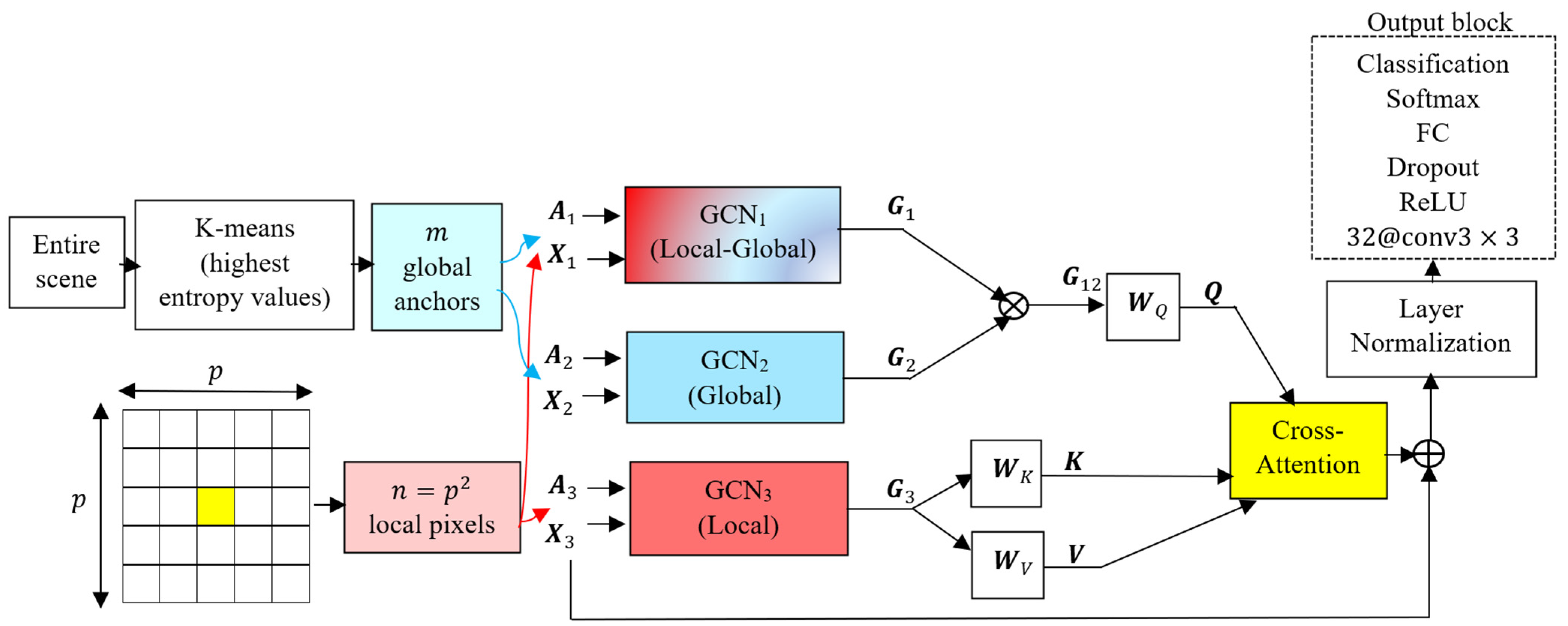
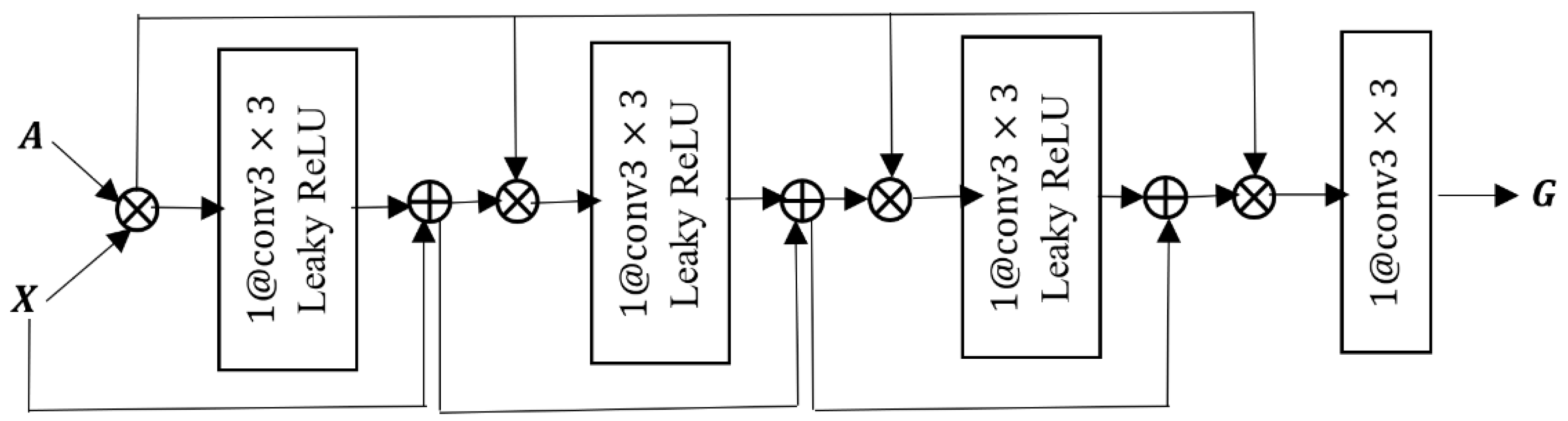
The block diagram of the proposed GF2 network is shown in Figure 1. Depicted are three graph convolutional networks (GCNs), each one taking two inputs, a feature matrix $\left(\mathit{X}\right)$, and an adjacency matrix $\left(\mathit{A}\right)$. The inner structure of the suggested GCN block is shown in Figure 2. The cross product in Figure 1 and Figure 2 represents the matrix product. In each GCN, the two inputs of the feature matrix $\mathit{X}$ and the adjacency matrix $\mathit{A}$ are multiplied. The result is passed through a convolutional layer containing one filter having a size of $3\times 3$, i.e., $1@\mathrm{c}\mathrm{o}\mathrm{n}\mathrm{v}3\times 3$, followed by a Leaky ReLU layer as a nonlinear activation function. The output of the first Leaky ReLU is added to the feature matrix $\mathit{X}$ through a residual connection, and the result is multiplied by the adjacency matrix $\mathit{A}$. This process is repeated three times, with the difference that in the second and third times, instead of $\mathit{X}$, the output of the previous additional layer is added to the output of the Leaky ReLU layer through the residual connection. The introduced GCN model is a series of operations in the following form:

$${\mathit{Z}}_{l+1}={\sigma }_l\left(\mathit{A}{\mathit{Z}}_l{\mathit{W}}_l\right)+{\mathit{Z}}_l$$

(2)

where ${\sigma }_l$ is the activation function (Leaky ReLU here), ${\mathit{Z}}_l$ is the feature matrix in layer $l$ $\left({\mathit{Z}}_1=\mathit{X}\right)$, and ${\mathit{W}}_l$ the learnable parameters of the convolutional filter. The output of the last multiplication operation is passed through a $1@\mathrm{c}\mathrm{o}\mathrm{n}\mathrm{v}3\times 3$ to provide the feature matrix of the graph $\left(\mathit{G}\right)$. In the remainder of this section, details of the three constructed graphs and their fusion are detailed.

2.1. Graph 1

The first graph explores the relationships between local pixels in a $p\times p$ patch and the $m$ global anchors, considering the feature matrix ${\mathit{X}}_1\in {\mathcal{R}}^{n\times m}$ and adjacency matrix ${\mathit{A}}_1\in {\mathcal{R}}^{n\times n}$. The elements of the feature matrix are obtained as follows:

$${\left({\mathit{X}}_1\right)}_{ij}={‖{\mathit{p}}_i-{\mathit{q}}_j‖}_2;i=\mathrm{1,2},\dots ,n;j=\mathrm{1,2},\dots ,m$$

(3)

where ${\left({\mathit{X}}_1\right)}_{ij}$ is the element $\left(i,j\right)$ in matrix ${\mathit{X}}_1$, ${\mathit{p}}_i\in {\mathcal{R}}^{d\times 1};i=\mathrm{1,2},\dots ,n$ is the $i$th pixel in the local patch, and ${\mathit{q}}_j\in {\mathcal{R}}^{d\times 1};j=\mathrm{1,2},\dots ,m$ is the $j$th global anchor. So, feature matrix ${\mathit{X}}_1$ contains the differences between pixels in a local neighborhood and the global anchors.

The inverse distance between feature vectors of each pair of nodes creates stronger connections between close nodes in the adjacency matrix. However, the regular distance is highly sensitive to small distances, as small changes in distance may result in larger changes in the computed adjacency weight. To deal with this issue, logarithmic scaling is used. The log transformation compresses large values and expands small values. Thus, it mitigates the extreme influence of very small distances in inverse-distance schemes. This enhances the global connectivity by avoiding fragmented graphs with disconnected or weakly connected components. This step makes the weights more uniform, improves the eigenvalue spectrum, and in turn smooths the spectrum of the adjacency matrix, enhancing training stability in the graph neural network. The elements of the adjacency matrix are computed as:

$${\left({\mathit{A}}_1\right)}_{ij}=\left|\log \left[\left({\displaystyle \frac{1}{{‖{\left({\mathit{x}}_1\right)}_i-{\left({\mathit{x}}_1\right)}_j‖}_2+1}}\right)+1\right]\right|$$

(4)

where $\left|·\right|$ represents the absolute value of its argument, ${\left({\mathit{x}}_1\right)}_i\in {\mathcal{R}}^{m\times 1}$ is the $i$th row of ${\mathit{X}}_1$, and ${\left({\mathit{A}}_1\right)}_{ij}$ is the element $\left(i,j\right)$ of matrix ${\mathit{A}}_1$. The quantity 1 in the denominator is added to avoid indefinite results with infinite values in the fraction. Therefore, in ${\mathit{A}}_1$, the difference among each pair of rows in the feature matrix ${\mathit{X}}_1$ is computed; ${\left({\mathit{x}}_1\right)}_i$ and ${\left({\mathit{x}}_1\right)}_j$ contain the differences between the $i$th and $j$th neighboring pixel within the local patch with the $m$ global anchors, respectively. If the two vectors ${\left({\mathit{x}}_1\right)}_i$ and ${\left({\mathit{x}}_1\right)}_j$ are similar, pixels at $i$ and $j$ inside the local patch have close similarities with the $m$ anchors, i.e., with the global representation of the image. If ${\left({\mathit{x}}_1\right)}_i$ and ${\left({\mathit{x}}_2\right)}_i$ are similar, they belong to the same cluster or class with higher likelihood.

2.2. Graph 2

The second graph is global and contains the relations among the $m$ anchors. The feature matrix of graph 2, indicated by ${\mathit{X}}_2\in {\mathcal{R}}^{m\times d}$, is represented by:

$${\mathit{X}}_2={\left[{\mathit{q}}_1{\mathit{q}}_2\dots {\mathit{q}}_m\right]}^{\mathrm{T}}$$

(5)

where ${\mathit{q}}_i\in {\mathcal{R}}^{d\times 1};i=1,\dots ,m$ is the feature vector of the $i$th anchor containing $d$ spectral features in the hyperspectral image and ${\left(·\right)}^{\mathrm{T}}$ denotes the transpose operation. The elements of the adjacency matrix of graph 2, ${\mathit{A}}_2\in {\mathcal{R}}^{m\times m}$, are derived as:

$${\left({\mathit{A}}_2\right)}_{ij}=\left|\log \left[\left({\displaystyle \frac{1}{{‖{\left({\mathit{x}}_2\right)}_i-{\left({\mathit{x}}_2\right)}_j‖}_2+1}}\right)+1\right]\right|$$

(6)

where ${\left({\mathit{x}}_2\right)}_i\in {\mathcal{R}}^{d\times 1};i=1,\dots ,m$ is the $i$th row of ${\mathit{X}}_2$ containing the spectral features of the $i$th anchor.

As graph 2 is global and does not contain information on the local patch centered at a given pixel, the feature matrix ${\mathit{X}}_2$ and adjacency matrix ${\mathit{A}}_2$ are the same for all pixels in the image.

2.3. Graph 3

The third graph is local and considers relationships between the $n$ pixels within a local patch. The feature matrix, ${\mathit{X}}_3\in {\mathcal{R}}^{n\times d}$, is represented by:

$${\mathit{X}}_3={\left[{\mathit{p}}_1{\mathit{p}}_2\dots {\mathit{p}}_n\right]}^{\mathrm{T}}$$

(7)

where ${\mathit{p}}_i\in {\mathcal{R}}^{d\times 1};i=\mathrm{1,2},\dots ,n$ is the $i$th pixel within the local patch centered around the given pixel. The elements of the adjacency matrix of graph 3, ${\mathit{A}}_3\in {\mathcal{R}}^{n\times n}$, are derived as:

$${\left({\mathit{A}}_3\right)}_{ij}=\left|\log \left[\left({\displaystyle \frac{1}{{‖{\left({\mathit{x}}_3\right)}_i-{\left({\mathit{x}}_3\right)}_j‖}_2+1}}\right)+1\right]\right|$$

(8)

where ${\left({\mathit{x}}_3\right)}_i\in {\mathcal{R}}^{d\times 1};i=1,\dots ,n$ is the $i$th row of ${\mathit{X}}_3$, ${{\left({\mathit{x}}_3\right)}_i=\mathit{p}}_i;i=1,\dots ,n$, i.e., the $i$th pixel within the local patch, and ${\mathit{A}}_3$ quantifies the similarities between pixels in the local patch.

2.4. Fusion of Graphs

The variables ${\mathit{X}}_1$ to ${\mathit{X}}_3$ and ${\mathit{A}}_1$ to ${\mathit{A}}_3$ are the inputs of the GCN blocks GCN₁ to GCN₃, where ${\mathit{G}}_1\in {\mathcal{R}}^{n\times m}$, ${\mathit{G}}_2\in {\mathcal{R}}^{m\times d}$, and ${\mathit{G}}_3\in {\mathcal{R}}^{n\times d}$ are the feature matrices obtained as output of GCN₁, GCN₂, and GCN₃. To combine the information of the feature maps of the three graphs, the features of the first two graphs are multiplied as follows:

$${\mathit{G}}_{12}={\mathit{G}}_1\times {\mathit{G}}_2$$

(9)

where ${\mathit{G}}_{12}\in {\mathcal{R}}^{n\times d}$ contains the combined information of graph 1 and 2. Therefore, the result of this multiplication is related to the dependencies of $n$ pixels based on their similarities (or differences) with respect to the global representatives (anchors). Subsequently, the two feature maps ${\mathit{G}}_{12}$ and ${\mathit{G}}_3$ should be combined. To this end, a cross-attention mechanism is suggested as follows.

The query component $\mathit{Q}\in {\mathcal{R}}^{n\times f}$ is obtained from ${\mathit{G}}_{12}$, while the component key $\mathit{K}\in {\mathcal{R}}^{n\times f}$ and the component value $\mathit{V}\in {\mathcal{R}}^{n\times f}$ are computed from ${\mathit{G}}_3$. Here, $f$ is the number of features in the projected feature space obtained by applying the projection matrices ${\mathit{W}}_Q\in {\mathcal{R}}^{d\times f}$, ${\mathit{W}}_K\in {\mathcal{R}}^{d\times f},$ and ${\mathit{W}}_V\in {\mathcal{R}}^{d\times f}$ (here we consider $f=d$). The obtained components are:

$$\mathit{Q}={\mathit{G}}_{12}{\mathit{W}}_Q$$

(10)

$$\mathit{K}={\mathit{G}}_3{\mathit{W}}_K$$

(11)

$$\mathit{V}={\mathit{G}}_3{\mathit{W}}_V$$

(12)

Note that ${\mathit{W}}_Q$, ${\mathit{W}}_K,$ and ${\mathit{W}}_V$ are the learnable parameters. The attended feature maps are derived as:

$${\mathit{G}}_{\mathrm{f}\mathrm{u}\mathrm{s}\mathrm{e}\mathrm{d}}=\mathit{V}\mathrm{s}\mathrm{o}\mathrm{f}\mathrm{t}\mathrm{m}\mathrm{a}\mathrm{x}\left({\displaystyle \frac{1}{\sqrt{f}}}{\mathit{Q}}^{\mathrm{T}}\mathit{K}\right)$$

(13)

where ${\mathit{G}}_{\mathrm{f}\mathrm{u}\mathrm{s}\mathrm{e}\mathrm{d}}$ is the fusion result of feature maps ${\mathit{G}}_{12}$ and ${\mathit{G}}_3$, which contains information of all three graphs. In other words, the similarity among the query component from ${\mathit{G}}_{12}$ and the key component from ${\mathit{G}}_3$ is computed through their scaled product, $\left({\displaystyle \frac{1}{\sqrt{f}}}{\mathit{Q}}^{\mathrm{T}}\mathit{K}\right)$, and is normalized by the softmax operation. Then, multiplication of the normalized weight with the value component $\mathit{V}$ from ${\mathit{G}}_3$ yields the weighted feature maps of graph 3 as the fusion result ${\mathit{G}}_{\mathrm{f}\mathrm{u}\mathrm{s}\mathrm{e}\mathrm{d}}$.

2.5. Output

After the fusion of feature maps of the three graphs through the cross-attention mechanism, the feature matrix of graph 3, ${\mathit{X}}_3\in {\mathcal{R}}^{n\times d}$, is added to ${\mathit{G}}_{\mathrm{f}\mathrm{u}\mathrm{s}\mathrm{e}\mathrm{d}}\in {\mathcal{R}}^{n\times f}$, where $f=d$ is enforced to enable the addition operation among them. The result, i.e., ${\mathit{X}}_3+{\mathit{G}}_{\mathrm{f}\mathrm{u}\mathrm{s}\mathrm{e}\mathrm{d}}$ is fed into the output block, which consists of $16@\mathrm{c}\mathrm{o}\mathrm{n}\mathrm{v}3\times 3,$ followed by the ReLU activation function and dropout, with a dropping probability of 0.2. Finally, the final part of the network is composed by a fully connected (FC) layer with $n_c$ neurons, where $n_c$ is the number of classes, a softmax, and a classification layer. The obtained label in output is assigned to the central pixel of the local patch in input to the network.

3. Results

3.1. Datasets and Parameter Settings

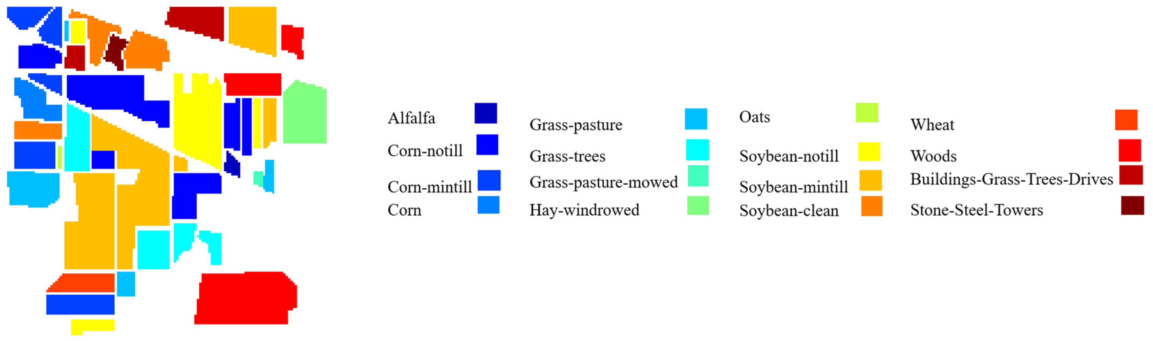
Three hyperspectral datasets are used in this section [40]. The Indian Pines dataset was collected in Northwestern Indiana in 1992 by the Airborne Visible/Infrared Imaging Spectrometer (AVIRIS). This hyperspectral image comprises 200 spectral channels in the spectral range of 0.4 to 2.5$\mathsf{\mu }\mathrm{m}$, after removal of 20 water absorption bands. The Indian Pines dataset has a nominal spectral resolution of 10 $\mathrm{n}\mathrm{m}$, a spatial resolution of 20 $\mathrm{m}$, 145 $\times$ 145 pixels, and 16 agricultural-forest labeled classes.

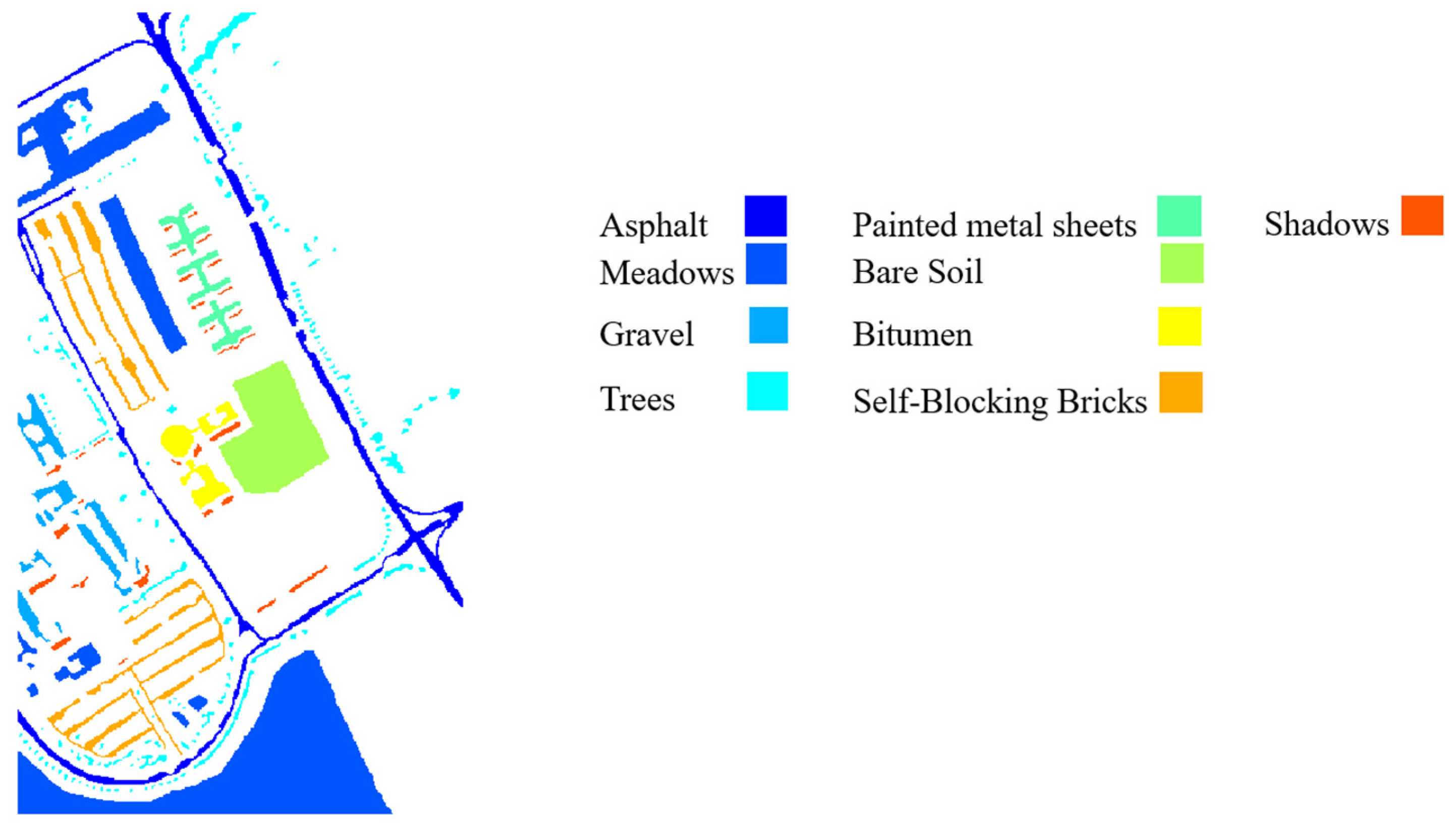
The University of Pavia dataset was acquired by the Reflective Optics System Imaging Spectrometer (ROSIS) in 2001. After the removal of noisy bands, the number of spectral channels is 103 in the spectral range of 0.43 to 0.86 $\mathsf{\mu }\mathrm{m}$. The University of Pavia dataset has a spectral resolution of 4 $\mathrm{n}\mathrm{m}$, a spatial resolution of 1.3 $\mathrm{m}$ per pixel, 610 $\times$ 340 pixels, and nine labeled semantic classes.

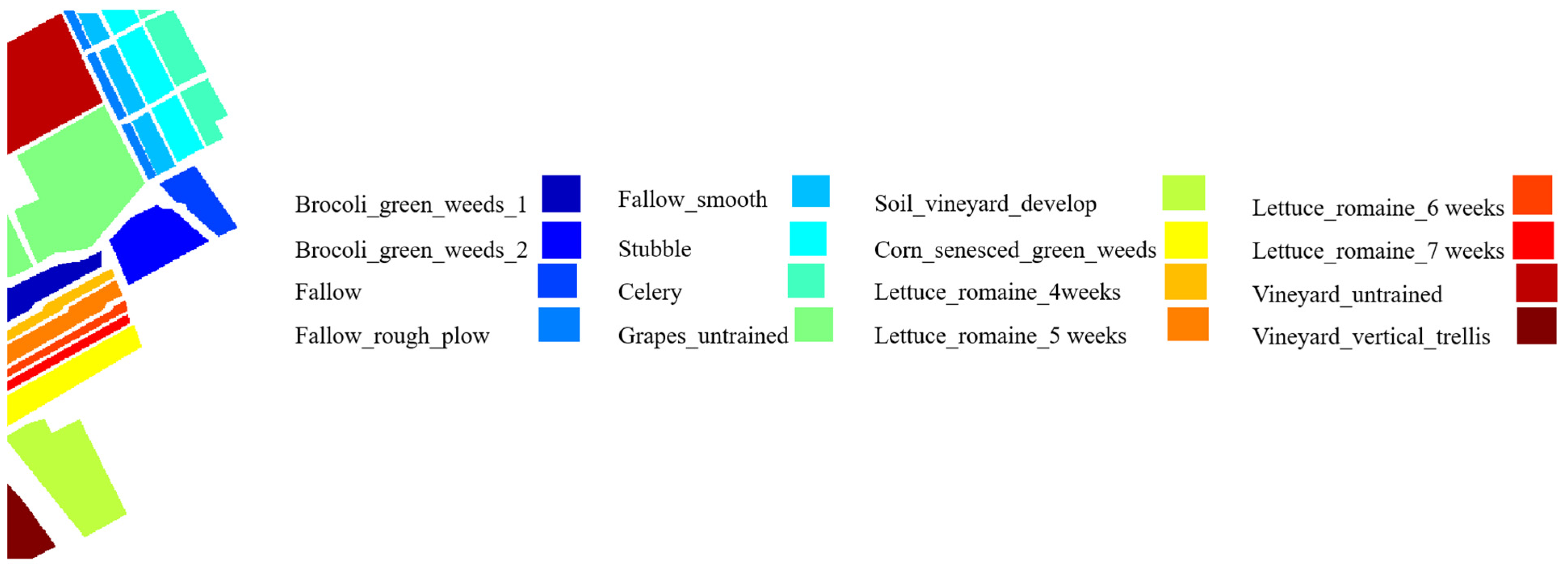
The Salinas dataset was collected over the valley of Salinas, Southern California, in 1998 by AVIRIS. It has 204 spectral channels in the range of 0.4–2.5 $\mathsf{\mu }\mathrm{m}$, after the removal of water absorption bands. This image has a nominal spectral resolution of 10 $\mathrm{n}\mathrm{m}$, with a ground sampling distance of 3.7 $\mathrm{m}$, 512 $\times$ 217 pixels, and 16 classes. The ground truth maps (GTM) of three datasets with associated legends are shown in Figure 3, Figure 4 and Figure 5.

In all datasets, 30 labeled pixels in each class are randomly chosen as training samples for classes containing more than 30 pixels, while 15 labeled pixels are considered otherwise. From the remaining samples, 5% are randomly chosen as validation data and the remaining are used as test samples.

The experiments are implemented on a laptop with Intel Core i5 and 32G RAM using MATLAB R2022b. The proposed network and the networks of all competitors are trained with Adam optimizer, an initial learning rate of 0.001, and 50 epochs. For the Indian Pines and Pavia datasets, the mini-batch size is set to 64, while for Salinas it is set to 16.

We conduct some preliminary experiments in order to set the spatial patch size $p\times p$, using the possible values $\left[5\times 5,7\times 7,9\times 9,11\times 11\right]$. Although a larger patch size would contain additional information, this could be unrelated to the central pixel, which may degrade the classification results. For the Indian Pines and Pavia datasets, a patch size of $7\times 7$ provides the highest accuracy, while in Salinas this happens for a size of $5\times 5$. Since more computational resources are required when increasing the patch size, we finally consider a catch-all value of $5\times 5$ for all cases.

We select a number of PCs containing 99% of the total variance in each dataset. The guided filtering [41,42] is applied for post-processing of the classification outputs of all methods (including, aside from the proposed method, the competitors SVM, SLIC-SVM, 2DCNN, Res2DCNN, 3DCNN, and Res3DCNN, which are introduced and discussed in the next sections). The first three PCs of the hyperspectral image are considered as a color guidance image. The filtering size $\left(2r+1\right)$ and the regularization parameter $\epsilon$ of the guided filter are set as follows: $r=5$ and $\epsilon ={10}^{-3}$ in Indian Pines, $r=17$ and $\epsilon ={10}^{-6}$ in Pavia, and $r=15$ and $\epsilon ={10}^{-3}$ in Salinas.

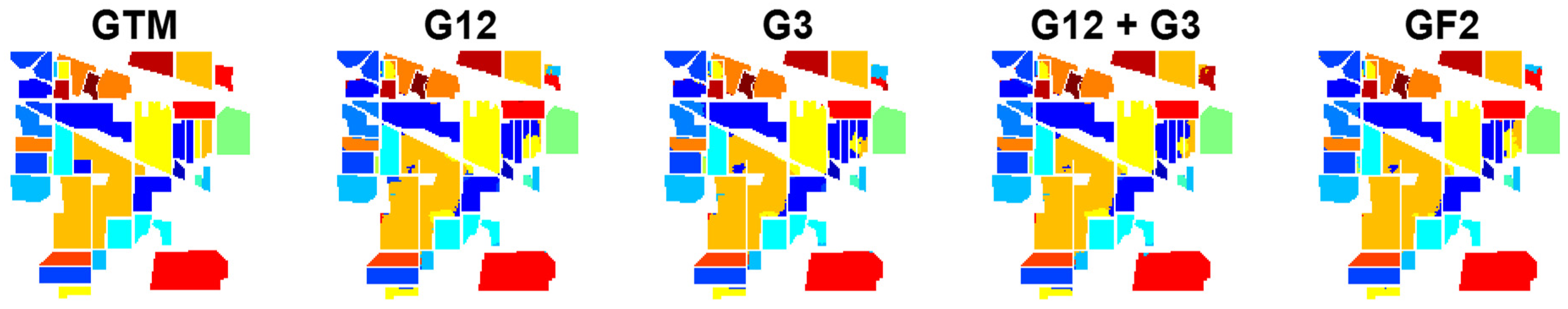
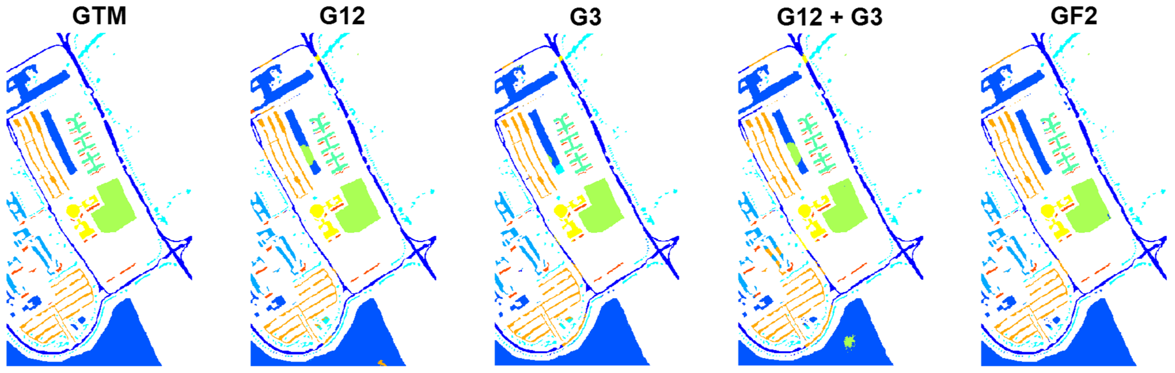
3.2. Ablation Study

To assess the performance of each part of the proposed network, the following cases are compared:

• G12: in this case, the feature map ${\mathit{G}}_{12}$, which is the multiplication of the outcomes of graphs 1 and 2 as outputs of the GCN₁ and GCN₂ blocks, respectively, is fed into the output block for classification.
• G3: in this case, the feature map ${\mathit{G}}_3$, which is the result of Graph 3 as output of the GCN₃ block, is fed into the output block for classification.
• G12 + G3: in this case, the feature maps ${\mathit{G}}_{12}$ and ${\mathit{G}}_3$ are fused through the addition operation, with the result fed into the output block.
• GF2: this is the main proposed method, where the feature maps ${\mathit{G}}_{12}$ and ${\mathit{G}}_3$ are fused through a cross-attention mechanism, with the result fed into the output block.

In

Table 1. Classification results for different network configurations for the Indian Pines dataset (the highest values of the values in the last two rows are highlighted in bold).

			G12		G3		G12 + G3		GF2
No	Name of Class	# Samples	Acc.	Rel.	Acc.	Rel.	Acc.	Rel.	Acc.	Rel.
1	Alfalfa	46	100.00	98.18	100.00	98.18	100.00	94.74	100.00	100.00
2	Corn-notill	1428	92.61	93.19	94.63	90.05	92.68	92.81	95.26	95.99
3	Corn-mintill	830	90.05	90.48	89.93	94.70	89.93	93.40	89.57	98.42
4	Corn	237	100.00	70.91	100.00	75.73	100.00	73.12	100.00	74.05
5	Grass-pasture	483	95.17	90.44	94.97	83.99	94.37	96.30	96.58	93.75
6	Grass-trees	730	99.06	99.73	98.66	99.86	98.93	100.00	100.00	98.55
7	Grass-pasture-mowed	28	96.15	80.65	96.15	80.65	96.15	80.65	96.15	80.65
8	Hay-windrowed	478	100.00	100.00	100.00	100.00	100.00	100.00	100.00	100.00
9	Oats	20	100.00	100.00	95.00	100.00	100.00	100.00	45.00	100.00
10	Soybean-notill	972	95.25	85.29	93.80	90.80	92.56	89.33	96.07	91.81
11	Soybean-mintill	2455	89.10	96.32	92.18	97.77	92.95	95.82	95.75	97.36
12	Soybean-clean	593	96.42	97.85	97.39	98.52	97.07	96.91	97.72	97.40
13	Wheat	205	100.00	98.15	100.00	97.25	100.00	98.60	100.00	100.00
14	Woods	1265	95.36	99.36	93.28	99.51	90.49	99.41	97.60	99.76
15	Buildings-Grass-Trees-Drives	386	100.00	96.20	100.00	95.00	100.00	78.51	100.00	99.48
16	Stone-Steel-Towers	93	100.00	95.96	100.00	95.96	100.00	95.96	100.00	95.96
Average accuracy and Average reliability (%)			96.82	93.29	96.62	93.62	96.57	92.85	94.36	95.20
Overall accuracy (%)			94.04		94.66		94.09		96.41
Kappa coefficient (%)			93.24		93.93		93.28		95.92

, the classification results for the four mentioned cases are reported for the Indian Pines dataset. In addition to accuracy (Acc.) and reliability (Rel.) [43] of each class, the average accuracy of classes, average reliability of classes, overall accuracy, and Kappa coefficient [44] are reported. To show that the difference between each pair of classifiers is statistically significant, McNemar’s test [45] is computed, and the obtained Z-scores are reported in

Table 2. Z-scores for different network configurations for the Indian Pines dataset.

	G12	G3	G12 + G3	GF2
G12	0	−4.08	−0.29	−104.14
G3	4.08	0	3.85	−103.52
G12 + G3	0.29	−3.85	0	−103.99
GF2	104.14	103.52	103.99	0

. In the results, GF2, with a significant difference with respect to the other methods, ranks first. After that, G3 provides the highest accuracy. The efficiency of G12 and G12 + G3 with some difference is similar, where the difference of G12 + G3 with respect to G12 is not statistically significant, according to the corresponding Z-score (Z = 0.29). The GTM and classification maps of different cases for the Indian Pines dataset are shown in Figure 6.

The classification results and the obtained Z-scores for the University of Pavia dataset are reported in

Table 3. Classification results for different network configurations for the University of Pavia dataset (the highest values of the values in the last two rows are highlighted in bold).

			G12		G3		G12 + G3		GF2
No	Name of Class	# Samples	Acc.	Rel.	Acc.	Rel.	Acc.	Rel.	Acc.	Rel.
1	Asphalt	6631	92.19	99.64	91.84	99.28	86.77	99.57	94.65	99.41
2	Meadows	18,649	95.31	98.85	97.17	99.36	94.85	99.47	99.83	98.74
3	Gravel	2099	100.00	97.13	100.00	96.64	84.85	98.13	100.00	97.95
4	Trees	3064	96.83	95.37	94.55	88.78	96.25	98.43	93.24	98.96
5	Painted metal sheets	1345	99.93	99.85	99.93	99.93	99.93	99.48	99.93	99.78
6	Bare Soil	5029	100.00	90.13	100.00	98.18	99.96	84.57	99.60	99.80
7	Bitumen	1330	100.00	91.16	100.00	90.05	100.00	84.28	100.00	97.08
8	Self-Blocking Bricks	3682	99.78	89.02	99.73	87.95	99.62	78.18	99.43	91.64
9	Shadows	947	87.54	94.63	89.65	99.88	88.49	99.88	89.33	99.88
Average accuracy and Average reliability (%)			96.84	95.09	96.99	95.56	94.52	93.55	97.33	98.14
Overall accuracy (%)			96.22		96.86		94.40		98.28
Kappa coefficient (%)			95.03		95.86		92.65		97.71

and

Table 4. Z-scores for different network configurations for the University of Pavia dataset.

	G12	G3	G12 + G3	GF2
G12	0	−7.66	18.46	−22.57
G3	7.66	0	22.18	−17.46
G12 + G3	−18.46	−22.18	0	−35.68
GF2	22.57	17.46	35.68	0

, respectively. Also, in this case, GF2 ranks first with a significant difference with respect to the other cases. Next, G3 and G12 provide the best results in this order, while G12+G3 provides the weakest classification results. The classification maps for the different configurations are shown in Figure 7.

The classification and McNemar’s test results for the Salinas dataset are reported in

Table 5. Classification results of different configurations for the Salinas dataset (the highest values of the values in the last two rows are highlighted in bold).

			G12		G3		G12 + G3		GF2
No	Name of Class	# Samples	Acc.	Rel.	Acc.	Rel.	Acc.	Rel.	Acc.	Rel.
1	Brocoli_green_weeds_1	2009	99.85	100.00	99.85	99.95	100.00	100.00	100.00	99.90
2	Brocoli_green_weeds_2	3726	100.00	99.92	100.00	99.92	100.00	99.57	100.00	100.00
3	Fallow	1976	100.00	100.00	100.00	99.60	99.95	100.00	100.00	100.00
4	Fallow_rough_plow	1394	97.78	99.27	98.64	99.13	99.00	98.71	99.64	99.07
5	Fallow_smooth	2678	99.66	97.02	99.37	97.62	99.40	97.94	99.63	99.03
6	Stubble	3959	99.82	100.00	99.82	100.00	99.82	100.00	99.80	100.00
7	Celery	3579	100.00	99.83	100.00	99.83	100.00	99.83	100.00	99.83
8	Grapes_untrained	11,271	99.07	99.11	98.76	99.60	98.38	98.37	99.41	99.92
9	Soil_vineyard_develop	6203	100.00	99.60	100.00	99.82	100.00	99.87	100.00	99.97
10	Corn_senesced_green_weeds	3278	97.38	96.20	98.47	96.91	99.05	95.92	99.24	96.64
11	Lettuce_romaine_4weeks	1068	100.00	100.00	99.91	95.95	100.00	99.53	98.88	100.00
12	Lettuce_romaine_5 weeks	1927	100.00	99.64	99.90	99.74	99.84	99.95	100.00	99.28
13	Lettuce_romaine_6 weeks	916	98.91	92.73	99.34	90.55	99.78	88.22	97.82	100.00
14	Lettuce_romaine_7 weeks	1070	88.88	93.69	86.07	95.84	82.99	97.37	93.46	96.62
15	Vineyard_untrained	7268	97.98	99.68	98.73	99.29	96.89	98.78	99.57	99.63
16	Vineyard_vertical_trellis	1807	100.00	100.00	99.78	100.00	100.00	100.00	100.00	100.00
Average accuracy and Average reliability (%)			98.71	98.54	98.67	98.36	98.44	98.38	99.22	99.37
Overall accuracy (%)			99.04		99.09		98.77		99.54
Kappa coefficient (%)			98.94		98.99		98.63		99.49

and

Table 6. Z-scores for different network configurations in the Salinas dataset.

	G12	G3	G12 + G3	GF2
G12	0	−1.76	7.76	−239.05
G3	1.76	0	9.59	−239.04
G12 + G3	−7.76	−9.59	0	−239.40
GF2	239.05	239.04	239.40	0

, respectively, and the corresponding classification maps are shown in Figure 8. As in the previous cases, GF2 ranks first, followed by G3 and G12 with a small difference between them, with a McNemar’s score of |Z| = 1.76 < 1.96, suggesting that the difference between these classifiers is not statistically meaningful.

The following results can be summarized from the reported results:

(1)

Although the performances of G12 and G3 are close, G3 provides slightly better classification results. As illustrated, G3 is the result of graph 3 containing relationships among pixels within a local patch; G₁₂ is the result of multiplying graphs 1 and 2, which quantify the similarity between the global anchors and, respectively, each pixel within the local patch and the global anchors themselves. This shows that considering local features within a neighborhood contains higher discriminative information compared to relationships between the local neighborhood and the global anchors selected from the entire scene.

(2)

Adding G12 and G3, i.e., G12+G3, generally results in weaker performance with respect to each of them taken separately. This implicitly means that the addition operation degrades the discriminative features of G12 and G3.

(3)

GF2, combining the feature maps G12and G3 through the cross-attention mechanism, yields the best classification results with a significant difference with respect to the other methods.

3.3. Comparison with Other Methods

In this section, the performance of the proposed GF2 network is compared with the following classifiers:

-

SVM: a pixel-based hard classifier where a third-order polynomial is used as a kernel function. In this paper, we use the LIBSVM implementation [46] with default parameters.

-

SLIC-SVM: a superpixel-based classifier. At first, the SLIC algorithm is applied to the first PC of the hyperspectral image and normalized in [0, 1] to provide a segmentation mask. Then, the obtained mask is applied to all PCs to provide the superpixels. The mean of the feature vectors in each superpixel is assigned to all pixels of that superpixel. Then, superpixels are classified using the SVM classifier with the same parameters used for classical SVM. In each dataset, the number of superpixels is set as $\left[{\displaystyle \frac{N}{{\left(p-1\right)}^2}}\right]$ [47], where $\left[·\right]$ denotes the nearest integer number, $N$ is the number of total pixels in the image, and $p$ is the spatial patch size.

-

2DCNN: a network composed of four convolutional layers, each of which contains $16@\mathrm{c}\mathrm{o}\mathrm{n}\mathrm{v}3\times 3$ filters with the “same” padding. Each layer is followed by a batch normalization (BN) and ReLU activation function. Moreover, after the second and fourth ReLU layers, a dropout layer with a dropping probability of 0.2 is used. The final part of the network is composed of FC, softmax, and classification layers.

-

3DCNN: the structure of this network is the same as 2DCNN, with the difference that two-dimensional convolutional layers $\left(16@\mathrm{c}\mathrm{o}\mathrm{n}\mathrm{v}3\times 3\right)$ are replaced by three-dimensional convolutional layers $\left(16@\mathrm{c}\mathrm{o}\mathrm{n}\mathrm{v}3\times 3\times 3\right)$.

-

Residual 2DCNN (Res2DCNN): the layers of this network are the same as 2DCNN, with the difference that three addition (add) layers are used after the first, second and third ReLU activation layers. The input is passed from $16@\mathrm{c}\mathrm{o}\mathrm{n}\mathrm{v}1\times 1$ and fed into the first addition (add1) layer through the residual connection. The output of add1 is fed into the second addition (add2) layer, and the output of add2 is in turn fed into the third addition (add3) layer through skip connections.

-

Residual 3DCNN (Res3DCNN): this network is the same as Res2DCNN, with the difference that it contains three-dimensional convolutional layers instead of two-dimensional ones.

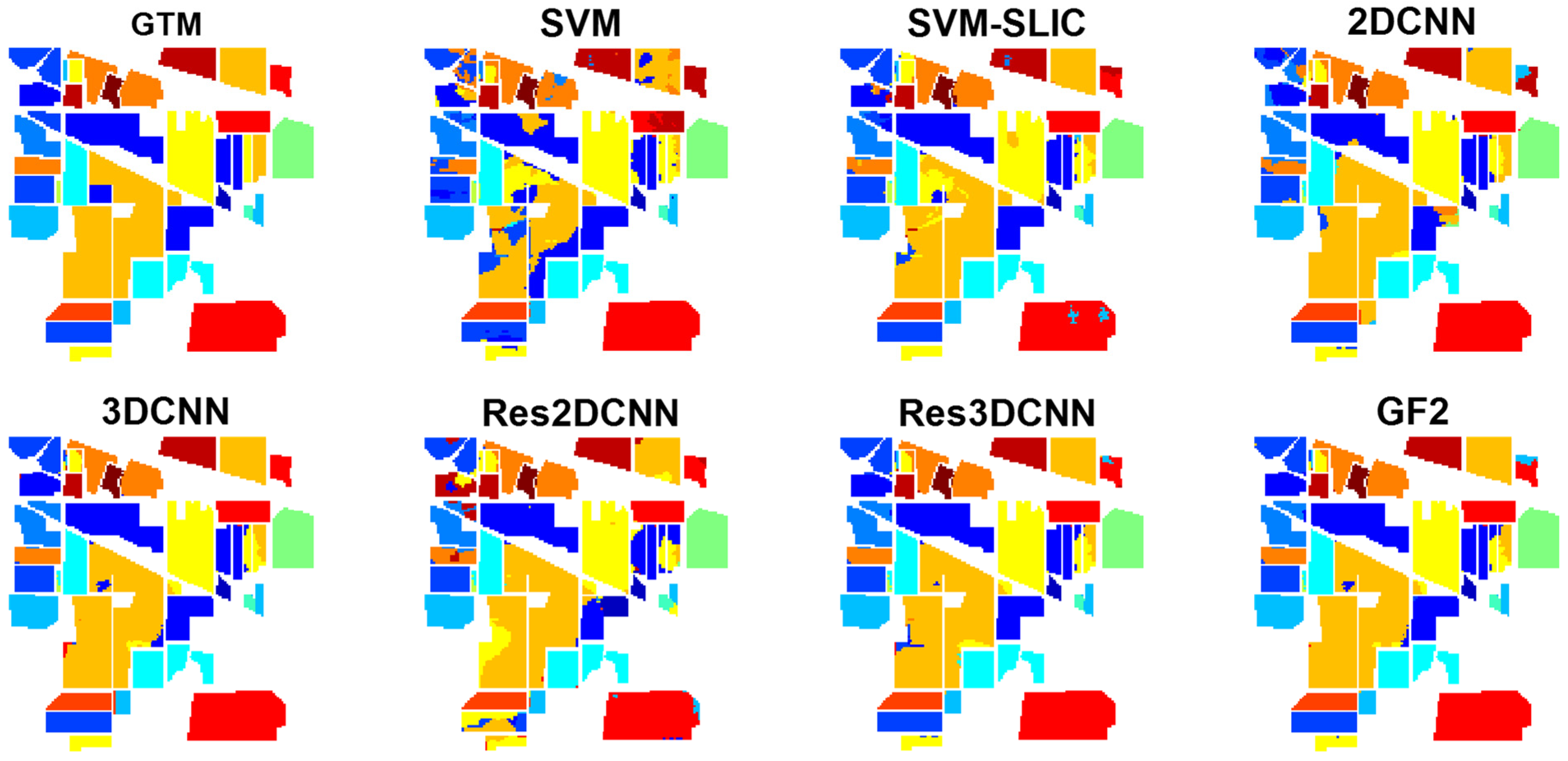
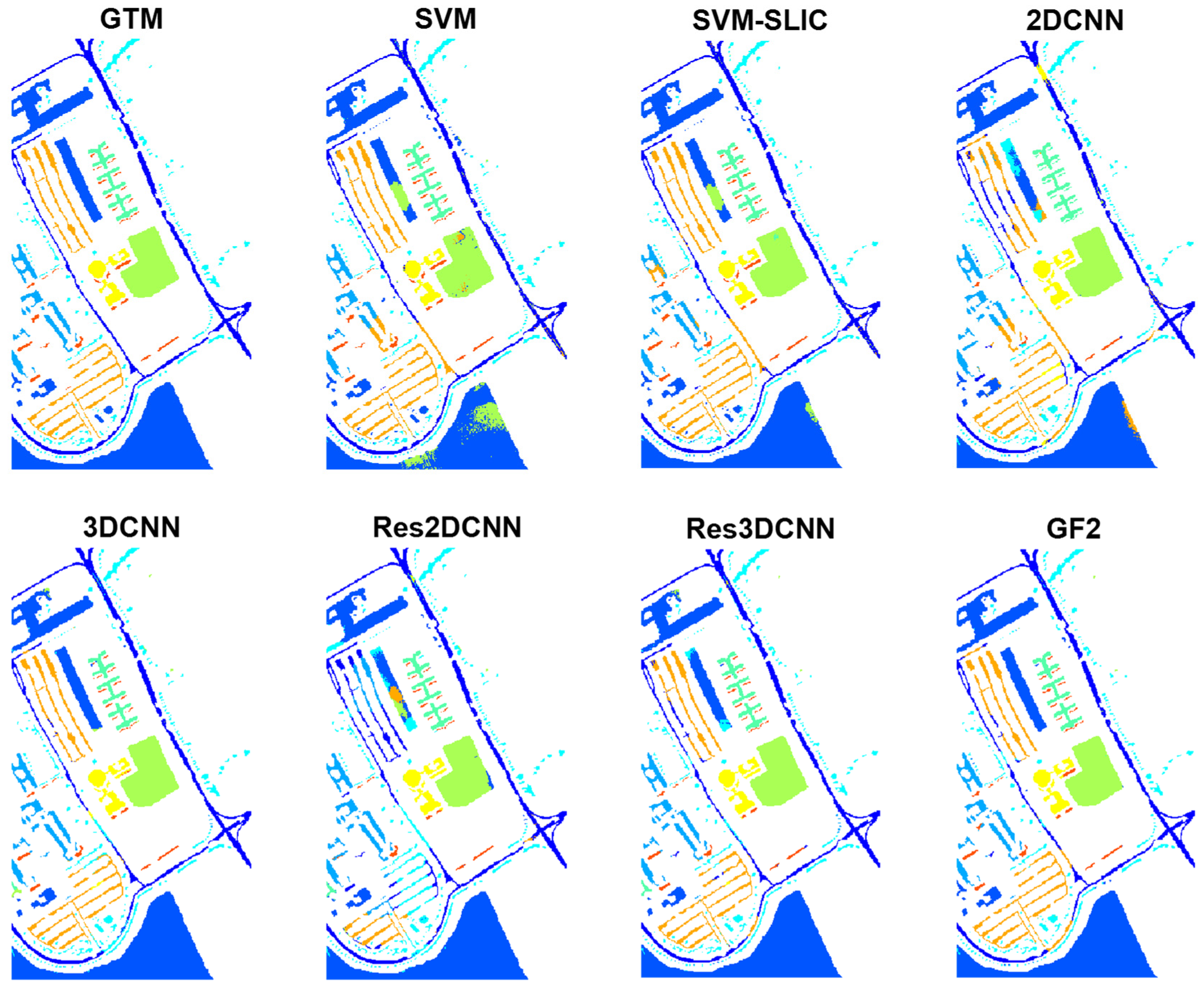
The classification results and associated Z-scores obtained by the McNemar’s test for Indian Pines are reported in

Table 7. Classification results of different methods for the Indian Pines dataset (the highest values of the classification measures in each row are highlighted in bold).

No	Name of Class	# Samples	SVM	SLIC-SVM	2DCNN	3DCNN	Res2DCNN	Res3DCNN	GF2
1	Alfalfa	46	100.00	100.00	100.00	100.00	100.00	100.00	100.00
2	Corn-notill	1428	85.36	93.58	84.73	95.75	71.83	94.14	95.26
3	Corn-mintill	830	74.22	94.24	71.70	89.69	62.59	89.81	89.57
4	Corn	237	100.00	100.00	100.00	100.00	100.00	100.00	100.00
5	Grass-pasture	483	94.97	98.59	79.68	93.76	89.13	97.18	96.58
6	Grass-trees	730	99.06	98.39	100.00	100.00	99.87	100.00	100.00
7	Grass-pasture-mowed	28	96.15	88.46	96.15	96.15	100.00	96.15	96.15
8	Hay-windrowed	478	100.00	100.00	99.80	100.00	100.00	100.00	100.00
9	Oats	20	95.00	95.00	50.00	50.00	50.00	45.00	45.00
10	Soybean-notill	972	96.07	93.90	95.66	97.62	91.94	95.66	96.07
11	Soybean-mintill	2455	64.95	89.10	96.35	93.76	85.90	93.11	95.75
12	Soybean-clean	593	85.02	91.21	92.02	97.88	93.65	97.72	97.72
13	Wheat	205	100.00	100.00	100.00	100.00	100.00	100.00	100.00
14	Woods	1265	79.98	94.51	90.96	99.92	96.75	98.84	97.60
15	Buildings-Grass-Trees-Drives	386	98.68	97.63	99.74	100.00	100.00	100.00	100.00
16	Stone-Steel-Towers	93	100.00	100.00	98.95	100.00	98.95	100.00	100.00
Average accuracy (%)			91.84	95.91	90.98	94.66	90.04	94.23	94.36
Overall accuracy (%)			83.43	93.97	91.63	96.33	87.57	95.79	96.41
Kappa coefficient (%)			81.39	93.16	90.47	95.83	85.92	95.22	95.92

and

Table 8. Z-scores of different methods for the Indian Pines dataset.

	SVM	SLIC-SVM	2DCNN	3DCNN	Res2DCNN	Res3DCNN	GF2
SVM	0	−28.75	−20.20	−34.14	−9.50	−32.77	−34.12
SLIC-SVM	28.75	0	7.48	−10.01	18.47	−8.07	−10.50
2DCNN	20.20	−7.48	0	−18.11	11.69	−15.86	−19.05
3DCNN	34.14	10.01	18.11	0	28.23	4.40	−0.68
Res2DCNN	9.50	−18.47	−11.69	−28.23	0	−27.07	−28.21
Res3DCNN	32.77	8.07	15.86	−4.40	27.07	0	−4.94
GF2	34.12	10.50	19.05	0.68	28.21	4.94	0

, respectively, with the corresponding classification maps shown in Figure 9. In general, GF2 provides the best classification results with a statistically significant difference with respect to all competitors except 3DCNN. Here, the fusion of local features of the neighborhood patches with the global information of the anchors results in a higher discrimination ability, and more accurate classification maps.

3DCNN and Res3DCNN rank respectively second and third, with a significant difference with respect to the other methods. The 3D convolutional layers simultaneously extract hierarchically spatial and spectral features from the three-dimensional image patch in input, leading to a separation of the different classes with high accuracy and reliability.

Following up, SLIC-SVM yields a satisfactory performance. On the one hand, the use of SLIC for providing superpixels considers spatial features in the neighborhood regions, and leads to smoothed classification maps with reduced noise. On the other hand, the use of SVM as a classifier with low sensitivity to the training set size can lead to highly accurate classification results.

Results from 2DCNN, Res2DCNN, and SVM are ranked next. Here, 2D convolutional networks applying 2D filters to explore the spatial features, thus ignoring the spectral information of the images, result in weaker performances compared to 3D filters. Similarly, the pixel-based SVM classifier just considers spectral features, and not considering the spatial information results in the worst classification results.

The classification results, Z-scores and classification maps obtained for the University of Pavia dataset are reported in

Table 9. Classification results of different methods for the University of Pavia dataset (the highest values of the classification measures in each row are highlighted in bold).

No	Name of Class	# Samples	SVM	SLIC-SVM	2DCNN	3DCNN	Res2DCNN	Res3DCNN	GF2
1	Asphalt	6631	91.52	93.15	85.22	93.62	92.31	95.37	94.65
2	Meadows	18,649	87.31	95.92	92.19	97.66	91.74	96.07	99.83
3	Gravel	2099	81.09	87.33	81.47	99.81	99.90	99.81	100.00
4	Trees	3064	88.41	93.73	98.76	97.26	95.33	97.52	93.24
5	Painted metal sheets	1345	99.48	99.93	99.48	99.85	99.93	99.93	99.93
6	Bare Soil	5029	96.06	99.03	99.92	99.98	97.87	99.98	99.60
7	Bitumen	1330	98.05	99.10	99.85	99.70	99.55	99.85	100.00
8	Self-Blocking Bricks	3682	98.59	99.48	80.45	94.02	19.93	92.26	99.43
9	Shadows	947	98.94	98.94	22.18	71.70	51.74	68.85	89.33
Average accuracy (%)			93.27	96.29	84.39	94.84	83.15	94.40	97.33
Overall accuracy (%)			90.71	95.88	89.87	96.63	86.64	96.02	98.28
Kappa coefficient (%)			87.93	94.57	86.79	95.55	82.53	94.76	97.71

and

Table 10. Z-scores of different methods for the University of Pavia image.

	SVM	SLIC-SVM	2DCNN	3DCNN	Res2DCNN	Res3DCNN	GF2
SVM	0	−41.35	4.47	−35.79	19.36	−31.04	−42.96
SLIC-SVM	41.35	0	35.99	−6.02	50.62	−1.06	−14.24
2DCNN	−4.47	−35.99	0	−47.37	18.57	−45.19	−53.77
3DCNN	35.79	6.02	47.37	0	61.94	8.33	−11.85
Res2DCNN	−19.36	−50.62	−18.57	−61.94	0	−59.12	−63.17
Res3DCNN	31.04	1.06	45.19	−8.33	59.12	0	−17.60
GF2	42.96	14.24	53.77	11.85	63.17	17.60	0

and Figure 10, respectively. The proposed GF2 generally yields the highest classification accuracy with a statistically significant difference with respect to other methods. SVM, which only uses spectral features, provides here better classification results compared to 2D convolutional networks, which explore the spatial features. This suggests that in this dataset, the spectral information is more relevant than the spatial information.

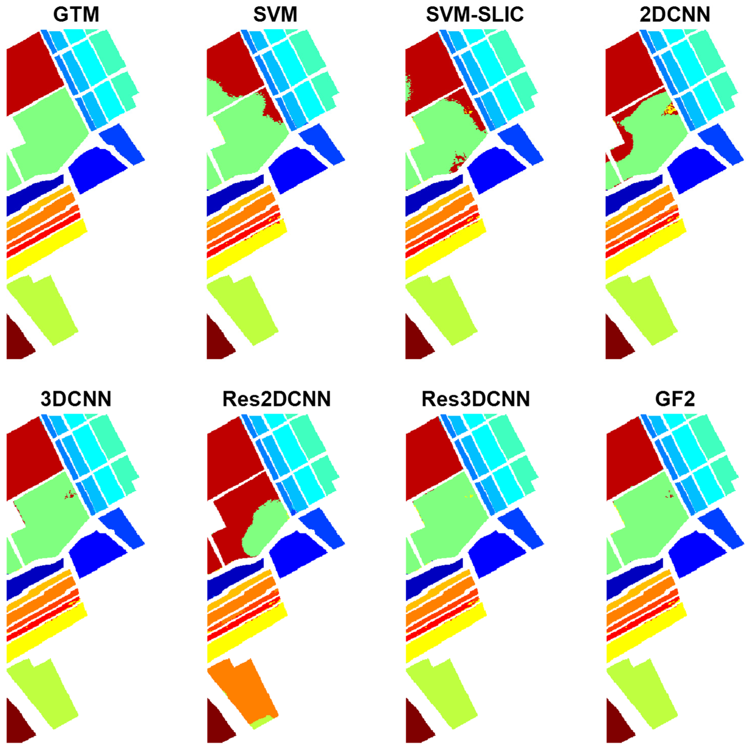
The classification accuracies and Z-scores related to the Salinas dataset are reported in

Table 11. Classification results of the different methods for the Salinas dataset (the highest values of the classification measures in each row are highlighted in bold).

No	Name of Class	# Samples	SVM	SLIC-SVM	2DCNN	3DCNN	Res2DCNN	Res3DCNN	GF2
1	Brocoli_green_weeds_1	2009	100.00	100.00	99.85	100.00	99.10	100.00	100.00
2	Brocoli_green_weeds_2	3726	100.00	100.00	100.00	100.00	100.00	100.00	100.00
3	Fallow	1976	100.00	100.00	100.00	100.00	100.00	100.00	100.00
4	Fallow_rough_plow	1394	100.00	100.00	99.64	98.21	93.69	99.86	99.64
5	Fallow_smooth	2678	98.58	98.81	99.37	99.63	99.51	99.44	99.63
6	Stubble	3959	99.87	99.90	99.90	99.80	99.85	99.87	99.80
7	Celery	3579	100.00	100.00	100.00	100.00	99.97	100.00	100.00
8	Grapes_untrained	11,271	92.24	86.08	81.40	99.09	32.09	99.28	99.41
9	Soil_vineyard_develop	6203	100.00	100.00	100.00	100.00	5.71	100.00	100.00
10	Corn_senesced_green_weeds	3278	97.96	98.44	99.18	99.27	99.27	99.24	99.24
11	Lettuce_romaine_4weeks	1068	97.85	98.88	97.47	98.97	98.88	98.97	98.88
12	Lettuce_romaine_5 weeks	1927	100.00	100.00	100.00	100.00	100.00	100.00	100.00
13	Lettuce_romaine_6 weeks	916	96.83	96.72	39.63	98.36	61.46	98.25	97.82
14	Lettuce_romaine_7 weeks	1070	96.07	94.67	94.39	91.96	94.11	86.26	93.46
15	Vineyard_untrained	7268	79.10	96.45	99.88	99.60	99.74	99.57	99.57
16	Vineyard_vertical_trellis	1807	100.00	100.00	100.00	100.00	100.00	100.00	100.00
Average accuracy (%)			97.41	98.12	94.42	99.06	86.46	98.80	99.22
Overall accuracy (%)			95.20	96.28	94.83	99.43	73.95	99.38	99.54
Kappa coefficient (%)			94.65	95.87	94.26	99.36	71.59	99.32	99.49

and

Table 12. Z-scores of the different methods for the Salinas dataset.

	SVM	SLIC-SVM	2DCNN	3DCNN	Res2DCNN	Res3DCNN	GF2
SVM	0	−12.44	3.09	−45.86	94.01	−44.79	−47.24
SLIC-SVM	12.44	0	13.24	−39.66	103.12	−38.36	−41.21
2DCNN	−3.09	−13.24	0	−48.42	103.98	−47.43	−49.67
3DCNN	45.86	39.66	48.42	0	117.05	1.78	−6.16
Res2DCNN	−94.01	−103.12	−103.98	−117.05	0	−116.41	−117.44
Res3DCNN	44.79	38.36	47.43	−1.78	116.41	0	−6.89
GF2	47.24	41.21	49.67	6.16	117.44	6.89	0

, respectively, and their classification maps are shown in Figure 11. Also here, GF2 ranks first with a significant difference with respect to all competitors. With a slight difference and low Z-score of |Z| = 1.78 < 1.96, 3DCNN and Res3DCNN denotes statistical mutual dependence in their results, and are ranked as the next best methods. The worst result is obtained by Res2DCNN.

The number of learnable parameters for the different networks are represented in

Table 13. The number of learnable parameters for different networks.

	2DCNN	3DCNN	Res2DCNN	Res3DCNN	GF2
No. of learnable parameters	17.1k	181.3k	16.2k	187.8k	162.6k

. Here, 2DCNN and its residual version are, in these terms, the lightest networks, having the lowest number of learnable parameters. However, 2DCNN and Res2DCNN cannot achieve accurate classification results across the different datasets. GF2, with about 163k learnable parameters, is still approximately a light network, imposing a reasonable computational burden. The 3DCNN and its residual version, Res3DCNN, have about 181k and 188k learnable parameters, respectively, and, in spite of this, underperform with respect to GF2. Therefore, the proposed GF2 results as a good candidate for hyperspectral image classification from both the classification accuracy and the computational complexity points of view.

4. Discussion

In this section, the performance of GF2 is discussed compared to several other graph-based neural networks.

Table 14. Comparison of GF2 with other graph-based networks.

	Method	GF2	Auto-GCN	Con-GCN	EMS-GCN	DAS-GCN	CAD-GCN	MDGCN	DIGCN
Indian Pines	OA	96.41	96.98	96.74	95.87	95.63	94.13	93.47	94.16
	Time (s)	49.87	60	-	23.02	860	62	95	53
Pavia	OA	98.28	95.55	95.97	98.47	96.40	92.91	95.68	93.24
	Time (s)	56.32	102	-	71.07	392	73	244	187
Salinas	OA	99.54	99.43	99.25	-	99.08	98.28	-	97.61
	Time (s)	1160.76	218	-	-	3410	826	-	616

reports the overall accuracy (OA) obtained by the different methods for the considered datasets, along with the running time (seconds) as reported from the respective references. In all cases, 30 training samples per class are used, or 15 for classes with less than 30 labeled samples. For each competitor, we report the highest achievable accuracy associated with the best parameter settings reported in its associated published reference. Because of different types of input data due to the different definition of the graphs, considering the same hyperparameters for all the different methods is not appropriate. For example, in Auto-GCN, rectangular regions of the image are considered as graph nodes, while in the proposed GF2 the graph nodes are defined as local pixels or global anchors. Thus, considering the same mini-batch size for these two methods is not reasonable because of the scale of the graph nodes, and the input size of the networks should be set differently. A brief description of the benchmark methods is represented next.

In the automatic GCN (Auto-GCN), both graph design and its learning are carried out by neural networks. A semi-supervised Siamese network is used to construct the high-order tensor graph, with an intersection over union (IoU) based metric introduced for relabeling the dataset. The GCNs, the Siamese network and classification network are jointly trained, which results in a meaningful graph representation.

In the contrastive GCN (ConGCN), a semi-supervised contrastive loss is designed to jointly extract supervision information from the scarce labeled data and the abundant unlabeled data. ConGCN uses a semi-supervised contrastive loss for exploiting the supervision signals from the spectral domain, and graph generative loss for exploring the spatial relations of the hyperspectral image, and simultaneously performs hierarchical and localized graph convolution to extract both global and local contextual information. Moreover, the use of an adaptive graph augmentation is suggested to improve the performance of contrastive learning.

The mixhop superpixel-based GCN (EMS-GCN) is an end-to-end superpixel-based GCN method. It utilizes a multiscale spectral-spatial CNN for feature extraction and an adaptive clustering distance for introducing an improved learning-based superpixel algorithm. In EMS-GCN, a mixhop superpixel-based GCN module is introduced for adaptive integration of local and long-range superpixel representation.

The context-aware dynamic GCN (CAD-GCN) does not limit the receptive field of GCN to a small region. Instead, it captures long-range dependencies through translating the hyperspectral image into a region-induced graph and encoding the contextual relations among different regions. Subsequently, CAD-GCN iteratively adapts the graph to refine the contextual relations among image regions.

The dynamic adaptive sampling GCN (DAS-GCN) dynamically refines the receptive field of each given node and corresponding connections through successively applying two complementary components in each round of the adaptive sampling. As a result, it exploits both spectral and spatial information from local neighbors and far image elements.

The multiscale dynamic GCN (MDGCN) utilizes a dynamic graph convolution instead of a fixed graph, which can be refined using the convolutional process of the GCN. In MDGCN, multiple graphs with different local scales are constructed to provide spatial information at different scales, with varied receptive fields. To mitigate the computational burden, the total number of image elements to process is lowered by grouping from homogeneous areas in superpixels, treating each of them as a graph node.

In the dual interactive GCN (DIGCN), the interaction of multiscale spatial information is used to refine the input graph. To this end, the edge information contained in one GCN can be refined by feature representation from the other branch, and results in benefits of multiscale spatial information. Moreover, the generated region representation is enhanced by learning the discriminative region-induced graph.

For the Indian Pines dataset, Auto-GCN, ConGCN and the proposed GF2 rank first to third, respectively, with a slight difference. The lowest overall accuracy is obtained by CAD-GCN and DIGCN. For the University of Pavia dataset, EMS-GCN and GF2 rank respectively first and second, and provide highly accurate classification results with a significant difference with respect to the other methods. For the Salinas dataset GF2, Auto-GCN, and ConGCN rank first to third, respectively. Although Auto-GCN and ConGCN are among the best methods for the Indian Pines and Salinas datasets, they do not work as well for the University of Pavia dataset. The proposed GF2 network exhibits instead high accuracy across all datasets, and shows a robust behavior both for the different images of the University of Pavia, and images dominated by agricultural fields (Indian Pines and Salinas), also characterized by a different spatial resolution.

From the running time point of view, DAS-GCN is the slowest method for all datasets. Despite that, it is not among the most accurate methods. For the Indian Pines dataset, EMS-GCN, GF2, and DIGCN are the fastest methods. For the University of Pavia dataset, GF2 has the lowest running time. After that, EMS-GCN and CAD-GCN are the fastest methods. For the Salinas dataset, the lowest running time is reported for Auto-GCN.

While the proposed GF2 network is trained in 50 epochs, the Auto-GCN is trained in 150 epochs. Because of the following reasons, the Auto-GCN has relatively high complexity in the training phase: (1) Auto-GCN performs multitask learning and performs collaborative training for the Siamese network, GCNs, and hyperspectral image classification. (2) To compute the node similarities, the dual-input Siamese network is implemented in a semi-supervised manner. (3) A pre-training phase is performed in Auto-GCN such that the parameters of its feature extractor are initialized with the parameters of the trained feature extractor in the Siamese network, obtained during the offline training. However, the reported running time is the computation time of the test phase, i.e., the prediction time of the classification map. In Auto-CGN, the graph nodes are the image regions, while in GF2, they represent local pixels or global anchors. So, in datasets such as Salinas that have a higher number of pixels, the prediction time of GF2, which has pixel-based nodes, is higher with respect to Auto-GCN, which has region-based nodes.

5. Conclusions

While most graph-based networks use a superpixel algorithm to compose the hyperspectral image nodes, a graph-based network is proposed in this work, utilizing the pixels within a local patch as nodes of local graphs, and anchors with the highest entropy selected from the whole image as nodes of a global graph. Three graphs are composed, their processed features are fused, and finally used for pixel-based classification. An ablation study is carried out to assess the performance of each graph. Finally, the proposed GF2 network is compared with the classic SVM classifier, two versions of pixel-based and superpixel-based networks, namely 2DCNN, 3DCNN, and their residual versions, and several graph convolutional networks. The experiments on three hyperspectral datasets show a high classification accuracy for GF2. Moreover, GF2 is a relatively simple method, characterized by a relatively low number of learnable parameters. Therefore, GF2 can be a robust candidate for hyperspectral image classification. However, GF2 is fully supervised and therefore cannot exploit unlabeled samples for classification, except for the global information estimated from the anchors. The extension of GF2 to allow a semi-supervised workflow will be the subject of our future work. Due to the definition of the individual graphs for the pixels under test, the prediction time increases for large datasets. Especially in that case, the global anchors should be selected from a sub-region of the scene to increase the correlation between local and global spectral-spatial features. These aspects will be studied in future works.