The Response Mechanism of Ecosystem Service Trade-Offs Along an Aridity Gradient in Humid and Semi-Humid Regions: A Case Study of Northeast China

Abstract

In the context of global climate change, the sensitivity of ecosystem services (ESs) and their relationships to aridity are increasing, and the areas affected by aridity continue to expand. Previous research has largely focused on ES changes in arid regions under intensified aridity conditions and has overlooked humid and semi-humid regions, which are more sensitive to water loss. In this study, we applied a generalized additive model (GAM) to analyze the nonlinear responses of ES trade-offs to aridity in humid and semi-humid regions. The results indicated that at an aridity index (AI) of approximately 0.26, the trade-off intensity of two ES pairs—carbon sequestration vs. water yield and habitat quality vs. water yield—reached a peak. Additionally, structural equation modeling (SEM) based on threshold partitioning revealed significant shifts in ES trade-off drivers below and above the AI threshold. In areas with AI < 0.26, worsening meteorological and soil conditions exacerbated ES trade-offs, whereas in areas with AI > 0.26, competition for water resources between human activities and vegetation became the primary driver of intensified trade-offs. These findings highlight the need for targeted management strategies to maintain ecosystem stability in humid and semi-humid regions and provide valuable guidance for responding to increasing aridity risks.

1. Introduction

Ecosystem services (ESs), defined as the products and services provided by ecosystems to humans [1], are crucial for human survival and development [2]. Humid and semi-humid regions account for approximately 58% of the global land area and play a vital role in ecological protection and economic development, which simultaneously support multiple ecological functions and ESs [3,4]. Northeast China (NEC) is primarily located in humid and semi-humid areas and has diverse and representative vegetation types, making it an important region for global climate change research [5]. With the intensification of global warming and the increased frequency of human activities, the impacts of climate change are evident in Northwest and Northeast China, including rising temperatures and uneven precipitation [6], as well as frequent floods in the south and droughts in the north [7], posing significant threats. Compared to arid regions, ecosystems in humid and semi-humid areas tend to rely more on stable water resources [8]. Due to their limited exposure to aridity, these areas have a lower adaptability to aridity and are less exposed to the negative impacts of aridity [9]. The World Meteorological Organization, in its first “Global Water Resources Status Report”, pointed out that aridity had become more intense and frequent in most parts of the world in 2021 [10]. Therefore, there is an urgent need to improve our understanding of how ecosystems in humid and semi-humid regions, particularly in NEC, respond to aridity to enhance the region’s adaptability in the context of intensifying aridity.

Aridity can affect the overall function of ecosystems by influencing individual ESs and their relationships. The relationships between ESs can manifest as trade-offs or synergies [11]. Synergies refer to processes in which two ESs mutually reinforce each other [11], thereby contributing to the overall benefits of ESs [12]. Conversely, trade-offs refer to a relationship in which the increase in one ES leads to a decrease in another [11], representing a key obstacle in the optimization of ecological resources [13]. Weakening these trade-offs can help balance the provision of multiple ESs, thereby enhancing ecosystem benefits [12]. As climate change intensifies, particularly the aggravation of drought phenomena, the trade-off mechanisms of ESs have become more complex, leading to declines in ecosystem stability and the uneven provision of ESs [14,15]. Notably, aridity has been shown to cause biodiversity loss [16], a reduction in total soil carbon [17], decreased water availability, and the further exacerbation of ES trade-offs [18], all of which may ultimately threaten regional ecological security. Hence, exploring the dynamics of ES trade-offs in the context of intensifying aridity is crucial for optimizing ecological management strategies.

Research indicates that ES trade-offs often exhibit a nonlinear relationship with various influencing factors (e.g., aridity), displaying threshold effects [18,19,20,21]. The aridity index (AI), which is calculated as 1 − precipitation/potential evapotranspiration, is widely employed to assess the degree of aridity and its impact on ecosystems [22]. When the AI exceeds a certain threshold, the stable state of the ecosystem may be suddenly disrupted, leading to the rapid degradation of ESs and directly or indirectly affecting ES trade-offs [18,23,24]. For example, in arid regions of China, productivity, soil fertility, and plant abundance exhibited sharp declines when the AI values reached approximately 0.7, 0.8, and 0.95, respectively [23]. These findings indicate that once aridity surpasses a certain threshold, rapid changes in ESs and their relationships occur [25], impacting the overall benefits derived from these ESs [4]. The methods used to reveal these thresholds can generally be categorized into linear approaches and nonlinear approaches. Among these, nonlinear approaches (e.g., the constraint line method [26] and generalized additive models (GAMs) [25]) are better suited for addressing the complex interaction networks within ecosystems. Thresholds obtained using the constraint line method only represent the maximum value that the dependent variable can achieve under the limiting effect of the independent variable [27] and lack explanatory power for fitted curves beyond these thresholds. In contrast, the GAM utilizes smoothing functions to fit data, enabling the accurate identification of nonlinear relationships and thresholds with high flexibility and interpretability [28]. This approach facilitates a more comprehensive understanding of the nonlinear response of ES trade-offs to aridity, including the identification of key thresholds [25].

Driver analysis is widely utilized to explore the effects of natural factors (e.g., soil, meteorology, and vegetation) and human activities on ES trade-offs [21,29]. These effects may change below and above the AI threshold [19]. However, most of the driver analyses in existing studies focus on the whole rather than threshold partitions [30]. Threshold-based driver analysis can reveal the mechanisms of drivers at different aridity levels, providing deeper insights into the dynamic changes in ES trade-offs. Currently, various methods are employed for driver analysis, including the correlation coefficient method [31], geographical detector [32], and structural equation modeling (SEM) [33]. Among these techniques, SEM can be used to estimate relationships between latent variables that are difficult to observe directly while also quantifying the direct and indirect effects of these variables on ES trade-offs. These advantages make SEM a powerful tool for uncovering the driving mechanisms of ES trade-offs at different aridity levels.

The present study aimed to explore the response mechanisms of ES trade-offs to aridity in humid and sub-humid regions in 2021, using NEC as a case study. The main research objectives were to (1) explore the distribution and correlation of four ESs in NEC, namely, CS, water yield (WY), soil retention (SR), and habitat quality (HQ); (2) understand the changing patterns of ES trade-offs under different aridity conditions and identify key thresholds; and (3) investigate the driving mechanisms and key driving factors of ES trade-offs.

2. Materials and Methods

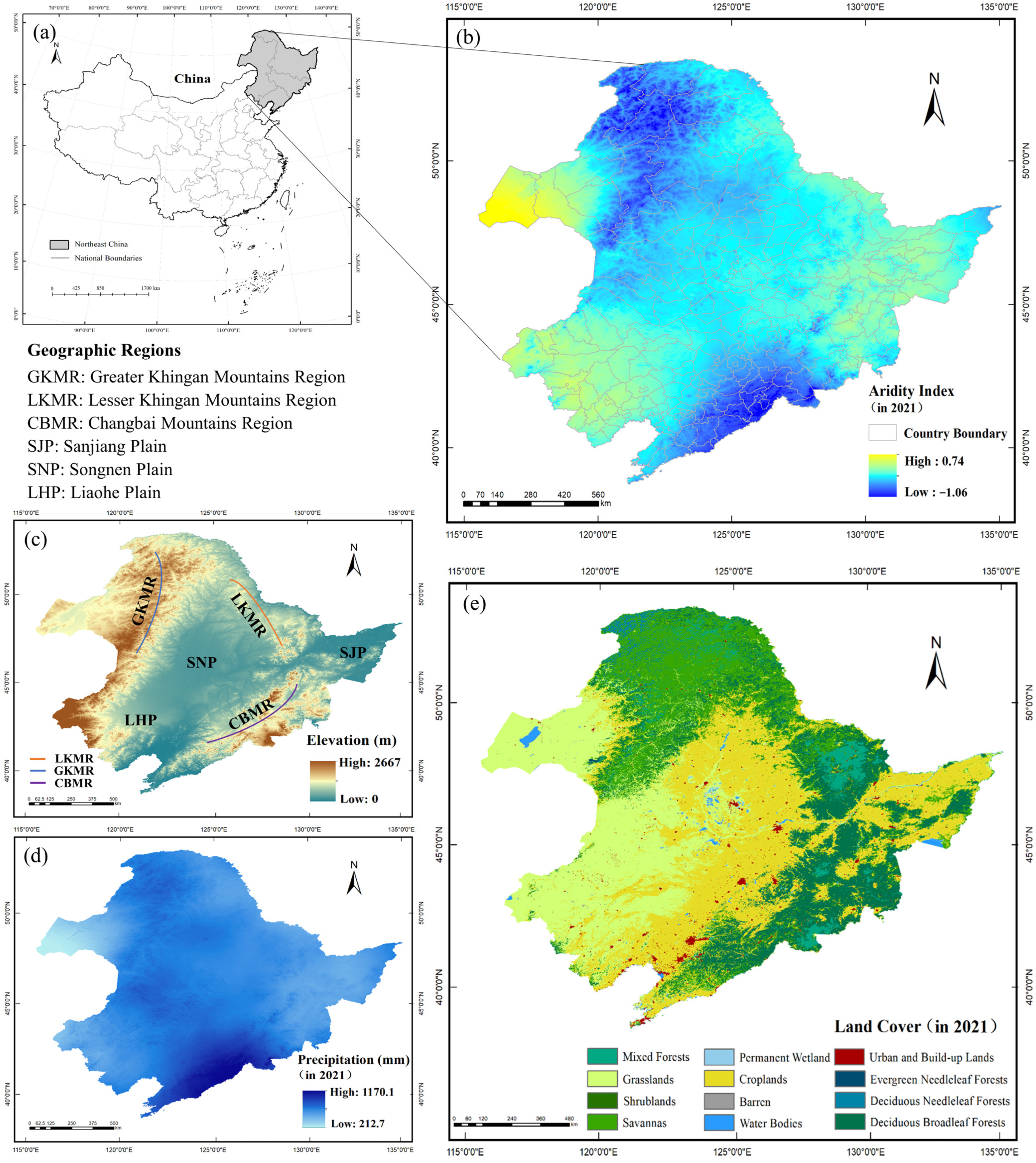
2.1. Study Area

The study area is located in NEC, with a total area of approximately 1.25 million km² [34], including Heilongjiang, Jilin, and Liaoning Provinces, and the eastern part of Inner Mongolia, containing a total of 226 counties (Figure 1b). From a geographical perspective, NEC mainly consists of three plains, namely, the Sanjiang Plain (SJP), Songnen Plain (SNP), and Liaohe Plain (LHP), as well as three major mountain ranges, namely, the Greater Khingan Mountain Region (GKMR), Lesser Khingan Mountain Region (LKMR), and Changbai Mountain Region (CMR) (Figure 1c). The study area has a predominantly temperate continental monsoon climate [35], with warm-temperate to mid-temperate and cold-temperate zones from south to north and an average annual temperature of 5.7 °C. NEC belongs to the humid and semi-humid zones and features an uneven spatial distribution of precipitation (Figure 1d). Precipitation mainly occurs in summer, with the annual precipitation ranging from 300 to 1100 mm. The dominant land cover types include mixed forests, cropland, and grasslands (Figure 1e) [36,37].

2.2. Data and Preprocessing

2.2.1. Topographic Data

The elevation data used in this study were derived from the ASTER GDEM v3 (Version 3 of the Advanced Spaceborne Thermal Emission and Reflection Radiometer Global Digital Elevation Model), which was obtained from the NASA website (https://www.earthdata.nasa.gov/news/new-aster-gdem/ (accessed on 1 May 2025)). The slope of the study area was determined using ArcGIS 10.8 (ESRI, Redlands, CA, USA).

2.2.2. Meteorological Data

Five types of meteorological data were obtained, namely, the monthly solar radiation data, monthly precipitation, average temperature, potential evapotranspiration data, and the AI in 2021. Monthly solar radiation data with a spatial resolution of 1/24° were obtained from the TerraClimate database (https://www.climatologylab.org/ (accessed on 1 May 2025)). Three types of meteorological data (i.e., the monthly precipitation [38], average temperature [39], and potential evapotranspiration data [40]) with a 1 km spatial resolution were provided by the National Tibetan Plateau Data Center (http://data.tpdc.ac.cn/ (accessed on 1 May 2025)). Based on the precipitation and potential evapotranspiration data, the AI was calculated using the following formula: 1 − precipitation/potential evapotranspiration [25]. This reflects the degree of climatic dryness, with higher values indicating drier conditions [25]. The resulting AI values are shown in Figure 1a.

2.2.3. Vegetation Data

The normalized difference vegetation index (NDVI) was derived from the MODIS MOD13Q1 (https://ladsweb.modaps.eosdis.nasa.gov/ (accessed on 1 May 2025)), with a spatial resolution of 250 m and a temporal resolution of 16 days. The monthly NDVI data were synthesized using the Google Earth Engine for research. The land use types were selected from the annual Type 1 data of the MODIS MCD12Q1 product, with a spatial resolution of 500 m (https://www.earthdata.nasa.gov/ (accessed on 1 May 2025)).

2.2.4. Soil Data

The soil data included a depth-to-bedrock map of China with a spatial resolution of 100 m [41], as well as four datasets obtained from the global gridded soil information SoilGrids v2.0 (https://www.isric.org/ (accessed on 1 May 2025)). These datasets included the sand, silt, clay, and soil organic carbon (SOC) contents, each with a spatial resolution of 250 m.

2.2.5. Human Activity Data

The population density and nighttime light index reflect the intensity of human activities [42]. In this study, population density data with a 1 km spatial resolution were obtained from the LandScan Global Population Database (https://landscan.ornl.gov/ (accessed on 1 May 2025)). Nighttime light data with a spatial resolution of 500 m were sourced from the Visible Infrared Imaging Radiometer Suite (VIIRS) on board the Suomi National Polar-Orbiting Partnership (S-NPP) satellite (https://eogdata.mines.edu/products/vnl/ (accessed on 1 May 2025)). In addition, the county-level administrative boundary data for NEC were obtained from the Geographical Remote Sensing Ecological Network Platform (http://www.gisrs.cn/ (accessed on 1 May 2025)) and covered a total of 226 counties (Figure 1b).

All raster data used in this study correspond to the year 2021 to ensure consistency in temporal coverage. To maintain spatial consistency, they were resampled to a resolution of 250 m within the boundary of the study area. Additionally, the coordinate system of all datasets was standardized to the Albers projection. Monthly scale datasets were processed according to model requirements: monthly solar radiation, monthly precipitation, and potential evapotranspiration were aggregated to annual totals; the average temperature was converted to an annual mean; and the monthly NDVI was composited using the maximum value method.

2.3. Methods

This study implemented a three-step process, as shown in Figure 2. First, CS, WY, HQ, and SR in NEC were quantified using the Carnegie–Ames–Stanford Approach (CASA) model, the annual water yield module of the Integrated Valuation of Ecosystem Services and Trade-Offs (InVEST) model, the habitat quality module of the InVEST model, and the Universal Soil Loss Equation (RUSLE), respectively (Objective 1). Second, the Spearman correlation coefficient was applied to clarify the relationships between ESs, and the GAM was employed to fit the response curves of ES trade-offs to the AI and identify the thresholds (Objective 2). Finally, based on threshold partitioning, SEM was conducted to analyze the drivers of ES trade-offs separately and to compare the differences in the driving pathways (Objective 3).

2.3.1. Quantification of ESs

In this study, four key ESs of NEC in 2021 were quantified as follows: CS, WY, HQ, and SR.

• CS

CS was quantified using the CASA model, a mechanistic model suitable for large-scale ecosystem carbon cycle research [32]. Net primary productivity (NPP) is a key indicator used to measure carbon sequestration in terrestrial vegetation [43]. The CASA model estimates the ecosystem NPP using remote sensing imagery and meteorological data based on the light use efficiency theory. The detailed principles underlying the CASA model can be found in previous studies [44]. The formula is as follows:

$$NPP\left(x,t\right)=APAR\left(x,t\right)\times \epsilon \left(x,t\right),$$

(1)

where $NPP\left(x,t\right)$ represents the NPP (g/m²) of pixel x in month t; $APAR\left(x,t\right)$ is the absorbed photosynthetically active radiation (PAR) (MJ/m²) of pixel x in month t; and $\epsilon \left(x,t\right)$ denotes the actual light use efficiency (g/MJ) of pixel x in month t. The detailed parameter settings for the CASA model are presented in Table S1.

• WY

WY was quantified using the Annual Water Yield module in InVEST 3.14 software. The model, which is based on the Budyko curve and the simplified water balance equation, utilizes spatial data (e.g., the annual precipitation) to estimate the actual evapotranspiration; it then calculates the difference between the precipitation and the actual evapotranspiration as the WY [45]. The relevant formulas are presented as follows:

$$WY\left(x\right)=\left(1-{\displaystyle \frac{AET\left(x\right)}{P\left(x\right)}}\right)\times P\left(x\right),$$

(2)

$${\displaystyle \frac{AET\left(x\right)}{P\left(x\right)}}=1+{\displaystyle \frac{PET\left(x\right)}{P\left(x\right)}}-{\left[1+{\left({\displaystyle \frac{PET\left(x\right)}{P\left(x\right)}}\right)}^{\omega }\right]}^{{\displaystyle \frac{1}{\omega }}},$$

(3)

where $WY\left(x\right)$ represents the Annual Water Yield (mm) for pixel x; $P\left(x\right)$ is the annual precipitation (mm) for pixel x; $AET\left(x\right)$ is the actual evapotranspiration (mm) for pixel x; $PET\left(x\right)$ is the potential evapotranspiration (mm) of pixel x; and $\omega$ is a non-physical parameter that characterizes the natural climate–soil characteristics. Further details are presented in Table S2.

• HQ

HQ was quantified using the habitat quality module in InVEST 3.14 software. The principle behind this approach is to determine the habitat suitability of the study area by assessing the condition and degradation of vegetation types, which is referred to as the HQ [45]. This method is suitable for multiscale ecological assessments. The formula is as follows:

$$Q_{xj}=H_j\times \left(1-\left({\displaystyle \frac{D_{xj}^z}{D_{xj}^z+k^z}}\right)\right),$$

(4)

where $Q_{xj}$ represents the habitat quality of pixel x in land use type j; $H_j$ denotes the habitat suitability of land use type j; $D_{xj}$ is the total stress level of pixel x in habitat type j; z is the scaling factor, which is commonly set to z = 2.5; and k is the half-saturation constant $Q_{xj}\in \left[0,1\right]$. Here, $Q_{xj}$ close to 0 indicates low HQ; and $Q_{xj}$ close to 1 indicates high HQ. Detailed parameter settings are presented in Tables S3 and S4.

• SR

The RUSLE was applied to quantify the annual SR as an evaluation indicator for SR [46]. This equation combines factors (e.g., rainfall erosivity, soil erodibility, and other variables) to estimate soil erosion, which is then used to estimate the SR capacity. This method is suitable for predicting soil erosion in different geographic regions [46]. The formula is as follows:

$$SR=R\times K\times L\times S\times \left(1-C\times P\right),$$

(5)

where SR represents SR (t/[hm²·a]); R is the rainfall erosivity factor (MJ·mm/[hm²·h·a]); K is the soil erodibility factor (t·hm²·h/[hm²·MJ·mm]); L is the slope length factor (unitless); S is the slope factor (unitless); C is the cover-management factor (unitless); and P is the support practice factor (unitless). Detailed parameters can be found in previous studies [47].

The quantitative indicators of different ESs have different orders of magnitude. Therefore, to eliminate dimensional differences between variables, the min–max normalization method was employed in this study to standardize the original values of the four ESs [19]. The validation methods for the quantification of the four ESs are provided in the Supplementary Material.

2.3.2. Relationships Between ESs

To further investigate the responses of ES trade-offs to aridity, the relationships between ESs were first identified, including the following six ES pairs: CS-WY, CS-SR, CS-HQ, HQ-WY, WY-SR, and SR-HQ. County-level administrative units are key participants in regional strategies and policies [48]. Therefore, this study used Spearman’s rank correlation coefficient to evaluate the strength of relationships between each ES pair at the county scale (i.e., the 226 counties shown in Figure 1a).

Spearman’s rank correlation is suitable for data with non-normal distributions and nonlinear relationships and is more effective in analyzing the complex interactions among ESs [31]. A positive Spearman’s correlation indicates a synergistic relationship, with higher values reflecting stronger synergy; conversely, a negative correlation suggests a trade-off relationship, with lower values representing stronger trade-offs. The correlation coefficient was used to quantify the intensity of ES trade-offs and synergies [49]. Because synergy is already considered the ideal state for sustainable development [19], this work focuses solely on ES trade-offs. In addition, to further explore how ES trade-offs respond to aridity, Spearman’s rank correlation was also used to calculate the correlation coefficients and significance levels between AI and each individual ES.

2.3.3. ES Responses to Aridity

Ecosystems are often characterized by complex, nonlinear intrinsic relationships due to the influence of various environmental factors. The GAM technique, as a flexible non-parametric regression method, captures the complex nonlinear relationships between variables through smoothing functions [28]. To further enhance the precision and robustness of the analysis, this study combined the moving window method (MWM) with the GAM method to explore the nonlinear relationships between ES trade-offs and AI.

After ranking the AIs of 226 counties in NEC, the MWM was used to calculate the mean AI and Spearman correlation coefficients between ESs within each window, effectively smoothing random fluctuations and increasing the sample size [50]. Subsequently, the GAM was employed to analyze the nonlinear relationships between the AI and ES trade-offs. This process was implemented using the “mgcv” package in R. The optimal window size was selected from a range of 50 to 90 based on higher R² values and lower Akaike information criterion (AIC) evaluation metrics [51]. Additionally, to support subsequent SEM [19], the mean values of the selected variables were calculated within each window.

2.3.4. Driver Analysis of ES Trade-Offs Based on the AI Threshold

SEM can be employed to estimate measurement errors and handle complex relationships between latent variables, making it commonly used in path analysis [33]. Partial least squares SEM (PLS-SEM) is particularly suitable for cases with small sample sizes, unknown data distributions, and complex model structures [52]. The present study divided model data based on the AI threshold obtained from the fitted GAM curves and then constructed PLS-SEM models below and above the AI threshold to explore the influences of vegetation, meteorological, soil, and topographic factors and human activities on ES trade-offs. These factors functioned as latent variables, while the data used to quantify ESs (introduced in Section 2.2) were used as observed variables in SEM.

In the SEM evaluation, the validity of the model was ensured at a Cronbach’s alpha and Dillon–Goldstein’s rho > 0.7, and structural model reliability was confirmed with loadings > 0.7 and communalities > 0.49 [33,53]. Manifest variable loadings should exceed cross-loadings to ensure discriminant validity, with a goodness-of-fit value > 0.7 ensuring a good model fit [54]. Following the model evaluation, several variables that failed to meet the criteria were removed (Tables S5 and S6). The final observed variables that were incorporated into the model are summarized in Tables S7 and S8.

3. Results

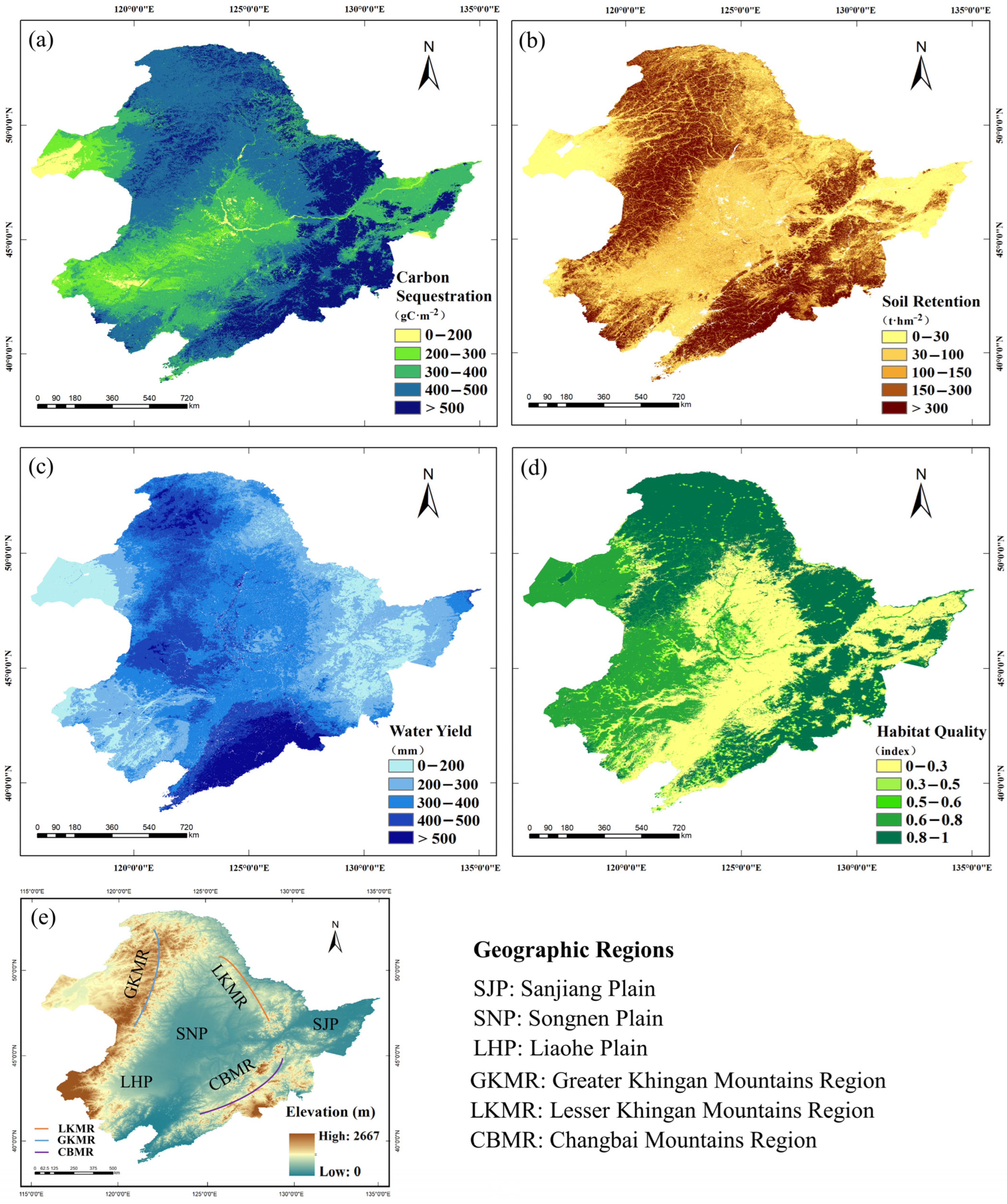
3.1. Spatial Patterns of ESs

The spatial distribution of CS, WY, SR, and HQ in NEC in 2021 is displayed in Figure 3. The spatial distribution pattern of CS (Figure 3) was, to some extent, related to land use types. High-value areas (>400 gC·m⁻²) were predominantly concentrated in mountainous regions (i.e., the GKMR, LKMR, and CMR) covered by forests. The CS in plain areas (i.e., the SNP, LHP, and SJP, as well as the eastern part of Inner Mongolia) was relatively low, with grassland and farmland dominating. The distribution of SR (Figure 3) was similar to that of CS. In terms of WY (Figure 3), high-value areas (>400 mm) were primarily identified in the GKMR and in southern coastal regions, while the eastern part of Inner Mongolia and the SJP exhibited a lower WY (<200 mm), which was closely related to the spatial distribution of precipitation in the same year. In addition, the HQ (Figure 3) varied in different vegetation-covered areas (i.e., forest-covered areas (>0.8), grassland-covered areas (0.5–0.8), and farmland-covered areas (<0.5)).

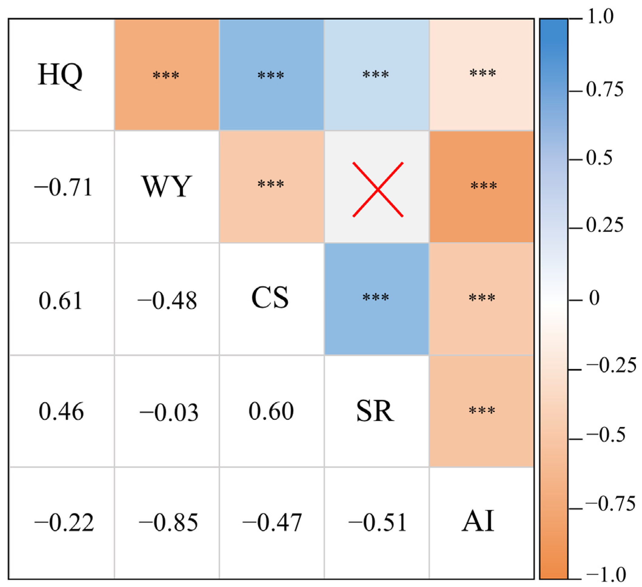
3.2. Analysis of ES Relationships

Except for the non-significant Spearman correlation between WY and SR, all other ES pairs exhibited significant correlations (CS-WY, CS-SR, CS-HQ, WY-HQ, and SR-HQ). Among them, the Spearman correlation coefficients for WY-HQ and CS-WY were −0.71 and −0.48, respectively, indicating significant negative correlations and, thus, trade-offs between these ESs. In contrast, CS-SR, CS-HQ, and SR-HQ showed significant positive correlations, with coefficients of 0.60, 0.61, and 0.46, suggesting synergies among these ESs. Most importantly, all four ESs (CS, WY, SR, and HQ) were significantly negatively correlated with the aridity index (AI), although the strength of these correlations varied (Figure 4).

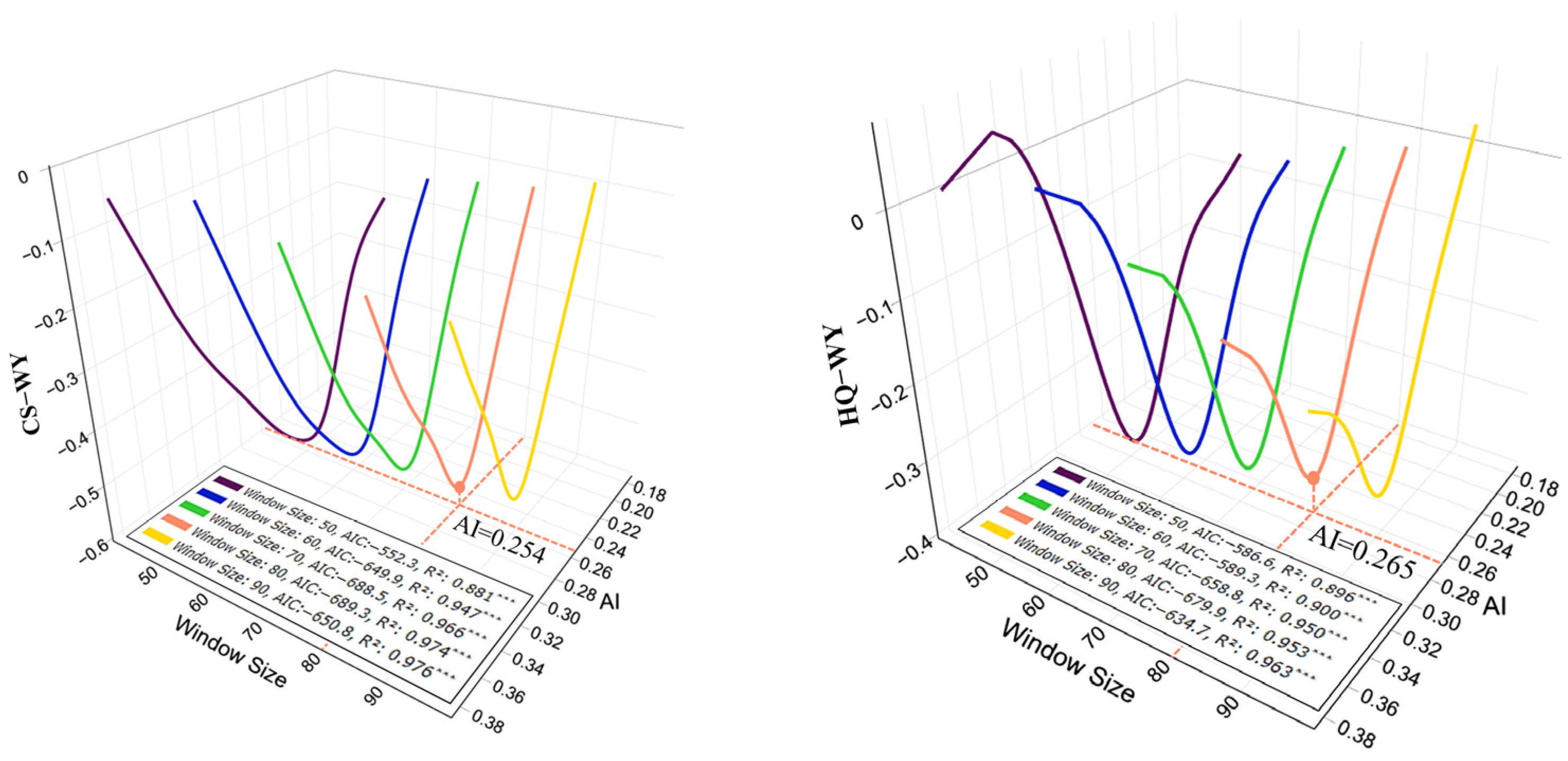
3.3. Response of ES Trade-Offs to Aridity

Using GAMs, this study analyzed the response of ES trade-offs to the AI. Figure 5 illustrates the response curves and AI thresholds for two ES pairs with trade-offs (CS-WY and HQ-WY). The trade-off intensity initially increased as the AI rose, peaking at an AI of 0.254–0.265, where correlation coefficients reached their minimum. Beyond this range, ES trade-offs gradually weakened as the AI increased. Based on these findings, this study utilized an average AI threshold of 0.26 for the further analysis of ES trade-off drivers.

GAM curves were tested with varying window sizes ranging from 50 to 90 (Figure 5). Despite changes in window size, the response patterns of CS-WY and HQ-WY to the AI remained consistent. At a window size of 80, the CS-WY curve achieved the best fit (R² = 0.974, AIC = −689.3) (Figure 5). Although the R² for HQ-WY at a window size of 80 was slightly lower than that at size 90, its AIC was significantly smaller (R² = 0.953, AIC = −679.9), indicating a better balance between the fit quality and model complexity. Thus, 80 was selected as the optimal window size for subsequent analysis.

3.4. Driver Analysis of ES Trade-Offs

The structural pathways of driving factors underlying ES trade-offs exhibited distinct patterns below and above the AI threshold (Figure 6), suggesting a fundamental shift in the internal driving mechanisms when the AI exceeded the critical level. The model achieved a goodness of fit of 0.91 for AI < 0.26 and 0.80 for AI > 0.26, both of which indicated strong model performance. The topographic factors shifted from having a negative effect (−0.97, p < 0.001) on meteorological factors to a positive effect (0.91, p < 0.001) above the threshold. Meteorological and soil factors also reversed their roles, changing from negative impacts (−0.86 and −0.54, respectively; p < 0.001) to positive impacts (0.41 and 0.33, respectively; p < 0.001) above the threshold. Though human activities shift from having non-significant to negative impacts on ES trade-offs (−0.28, p < 0.001) as AI increases, their influence on vegetation transitions from negative to non-significant (−0.27, p < 0.001). Additionally, the influence of vegetation on ES trade-offs shifts from positive (0.47, p < 0.001) to negative (−0.53, p < 0.001) with increasing AI values. These findings highlight the complex and dynamic mechanisms governing ES trade-offs across the AI threshold.

4. Discussion

4.1. Effects of Aridity on ES Trade-Offs

Vegetation can ensure HQ and provide CS by fixing atmospheric CO₂ through photosynthesis [55,56], but plant transpiration consumes a large amount of water. Therefore, the CS-WY and HQ-WY pairs exhibited ES trade-offs (Figure 4). Ecosystem indicators (e.g., vegetation cover) typically respond nonlinearly to increasing aridity. Once aridity surpasses a certain threshold, these responses shift accordingly [25]. With a slight increase in aridity, vegetation adapts by reducing leaf area and shedding leaves to conserve water [57,58]. These water-saving measures reduce vegetation photosynthesis and water consumption, leading to decreases in CS and HQ and an increase in WY, thereby intensifying the ES trade-offs (Figure 5). When the AI exceeds 0.26, the intensification of aridity may directly reduce WY, while the simultaneous declines in CS, HQ, and WY weaken ES trade-offs, consistent with Hu et al. [19].

NEC, located in humid and semi-humid regions, is generally not considered at risk of aridity. However, the sensitivity of vegetation to aridity is increasing globally, as all types of vegetation are susceptible to water stress [59]. Even in humid regions, the coupling between vegetation and aridity is growing stronger [60]. Hu et al. found the highest sensitivity on the Loess Plateau when the AI was around 0.5, with trade-offs (i.e., CS-WY and HQ-WY) shifting from intensification to weakening beyond this threshold [19]. However, the aridity threshold of NEC in the present study was 0.26, which is lower than that of the Loess Plateau, suggesting that vegetation in NEC may be more sensitive to aridity than that in the Loess Plateau [61]. Vegetation in humid regions is more sensitive to aridity due to limited aridity adaptability, while vegetation in arid regions has developed stronger aridity resistance through mechanisms such as leaf trait adjustments [62,63].

4.2. Drivers of ES Trade-Offs

Topography, a fundamental site condition, regulates ecosystem functions by shaping local hydrothermal environments and indirectly influencing ES relationships [29,64,65]. The results showed that topography positively affects ES trade-offs through meteorological factors, but the underlying pathways diverged considerably between humid (AI < 0.26) and arid (AI > 0.26) regions (Figure 6). In humid areas, elevated terrain promotes orographic precipitation and reduces evapotranspiration [66], increasing the precipitation-to-evapotranspiration ratio and mitigating aridity. These changes indirectly enhance water yield. At the same time, rugged topography limits human disturbance, thereby increasing CS and HQ levels and ultimately weakening ES trade-offs. Conversely, in arid areas, elevation has a limited influence on precipitation formation. Instead, dry air and suppressed moisture circulation exacerbate aridity [67,68], constrain vegetation growth, and lead to a synchronous decline in multiple ESs, resulting in weaker trade-offs. These contrasting mechanisms underscore how the role of topography in shaping ES trade-offs is contingent on regional climatic context.

Vegetation forms the foundation of ecosystems, supporting and affecting various ESs and their relationships through their ecological regulatory functions [69]. For example, vegetation can affect WY by regulating water use and directly influences the CS capacity of ecosystems through photosynthesis, contributing to maintaining habitat quality [57,70,71]. In relatively humid regions (AI < 0.26), abundant water promotes vegetation growth, which increases transpiration and enhances soil water retention through improved canopy cover and root structures [55,72]. These processes collectively support higher levels of CS and HQ and dampen ES trade-off intensity. Conversely, in relatively arid areas (AI > 0.26), although vegetation enhances CS, it also significantly increases water demand. In water-limited environments, additional vegetation consumes more water [73], intensifying competition for this scarce resource and ultimately exacerbating ES trade-offs. These contrasting mechanisms underscore the climate-dependent role of vegetation: it intensifies ES synergy under favorable conditions but becomes ineffective when constrained by water scarcity.

Human activities consistently exacerbate ES trade-offs, but their mechanisms differ significantly between relatively humid (AI < 0.26) and arid (AI > 0.26) regions. In humid areas, human activities—mainly urban expansion and surface hardening—reduce vegetation cover [74], which, in turn, limits photosynthesis and habitat quality (CS and HQ), indirectly intensifying ES trade-offs by disrupting ecological processes (Figure 6). In contrast, in arid areas where water is already scarce, human activities such as agriculture and groundwater extraction further deplete water resources [74]. This direct pressure worsens water scarcity and reduces ESs simultaneously, thereby increasing ES trade-offs (Figure 6). Overall, while both pathways increase trade-offs, their mechanisms shift from vegetation-related disturbance in humid zones to water competition in arid zones.

Soil plays a crucial role in ecosystem functions by regulating key processes, such as nutrient cycling and water availability, which directly influence plant growth and WY [75,76]. The mediating effect of soil is largely dependent on regional moisture conditions. In relatively arid regions (AI > 0.26), increases in soil organic carbon (SOC) and silt content enhance soil water retention and improve plant water availability, which, in turn, boosts photosynthetic efficiency [77,78]. This promotes higher levels of CS and HQ, reduces competition for water resources, and ultimately weakens ES trade-offs (Figure 6). In contrast, in relatively humid regions (AI < 0.26), although higher SOC also improves soil moisture retention and resilience to dryness [79,80], its contribution is limited in water-abundant areas. Instead, elevated SOC promotes vegetation growth and photosynthesis, which leads to greater transpiration, intensifies water use, and ultimately strengthens ES trade-offs (Figure 6). In summary, while SOC and silt contribute positively to ecosystem functioning in both climatic contexts, their effects on ES trade-offs differ; in arid regions, soil factors alleviate trade-offs by improving resource use efficiency, whereas in humid regions, excess vegetation growth enhances water loss through transpiration, thereby intensifying trade-offs.

The pathway through which meteorological factors indirectly influence ES trade-offs via vegetation and soil differs across regions with different aridity conditions. In both relatively humid (AI < 0.26) and relatively arid (AI > 0.26) areas, meteorological factors such as the aridity index and temperature have negative impacts on vegetation and soil. However, their effects on ES trade-offs follow different patterns (Figure 6). In relatively humid regions, although increased aridity and temperature reduce WY directly, CS and HQ remain relatively stable due to the resilience of vegetation [81]. As a result, ESs respond asynchronously to meteorological factors, leading to increased ES trade-offs. In contrast, in relatively arid regions, ecosystems are more fragile, and vegetation is less able to cope with climate stress [25,81]. Increased aridity and temperature not only continuously reduce WY but also impair the capacity of vegetation to sustain CS and HQ, leading to simultaneous declines in multiple ESs [19,25]. This synchronous decline reduces the differences in the ES responses to meteorology, thereby weakening the observed trade-offs. Thus, although meteorological factors affect ecological processes in similar ways, their effects on ES trade-offs vary significantly under different aridity conditions, highlighting the critical value of aridity threshold partitioning in ES response analyses.

4.3. ES Policy Implications and Limitations

This study is of great significance for understanding the drought response mechanisms of ecosystems in humid and semi-humid regions under climate change. Humid and semi-humid regions play critical roles in supporting multiple ecological functions and services [4], making these regions essential for global environmental stability. The findings of this study demonstrate that humid and semi-humid regions are highly sensitive to drought, indicating that these regions may face greater ecological risks under intensifying aridity (Figure 5). Therefore, future policies should place equal emphasis on humid and semi-humid regions, establishing early warning systems to address the potential impacts of drought. Additionally, regions with AI ≈ 0.26 exhibit the strongest ES trade-offs (Figure 5), highlighting their ecological instability and vulnerability to aridity. These areas should serve as critical indicators for drought alerts and should be prioritized for monitoring and management. As the AI changes, the influences of meteorology, soil, topography, vegetation, and human activities on trade-offs also shift (Figure 6). Thus, it is necessary to implement targeted ecological management strategies in areas below and above the AI threshold. Overall, this study provides a scientific foundation for drought response strategies in humid and semi-humid regions, which will ensure the stability of ecosystems under future climate change.

This study offers several avenues for future expansion and improvement. First, ES relationships are influenced by scale effects [82]. The county-level analysis performed in this study identified significant trade-offs between CS and WY, as well as between HQ and WY. However, these relationships may vary at finer spatial scales [83]. Future research should, therefore, consider multiple spatial scales to provide a more comprehensive perspective. Second, this study employed the InVEST model, the RUSLE, the water balance equation, and the InVEST model to assess four ESs. These models primarily relied on satellite data, which may reduce accuracy. To enhance the precision of these assessments, future studies should incorporate more field data to calibrate and validate model parameters. Finally, the current relationship analysis focused on ES pairs. In future research, more advanced methods should be applied to evaluate interactions among multiple ESs [84], thereby providing a deeper understanding of dynamic ES relationships. Despite these limitations, this study establishes an important foundation for aridity response strategies in humid and semi-humid regions, on which future studies can build further.

5. Conclusions

This study investigated the response mechanisms of ES relationships to aridity in humid and semi-humid regions of NEC, providing critical insights for ecological conservation and early warning systems. The results revealed significant trade-offs between CS and WY and between HQ and WY. These trade-offs exhibited a nonlinear response to increasing AI values, intensifying initially and then diminishing as the AI rose. ES trade-offs peaked at an AI threshold of approximately 0.26. The results showed that below this threshold (AI < 0.26), ES trade-offs were primarily driven by meteorological and soil factors, while above this threshold (AI > 0.26), the interplay between human activities and the demand for vegetation for water resources became the dominant factor. Therefore, for regions with an AI threshold < 0.26, interventions should focus on mitigating meteorological and soil degradation, whereas for regions with an AI threshold > 0.26, balancing human activities and vegetation water demand is crucial. The results of the present study highlight the importance of AI values approaching 0.26 as a critical signal for the early warning of drought. Additionally, the findings suggest that humid and semi-humid regions exhibit heightened sensitivity to aridity, with aridity thresholds emerging earlier compared to arid and semi-arid regions. Thus, paying early attention to the potential for aridity in humid and semi-humid regions is essential for buffering against the impacts of future climate change.

References

1. Millennium Ecosystem Assessment. Ecosystems and Human Well-Being: Synthesis; Island Press: Washington, DC, USA, 2005. [Google Scholar]
2. Costanza, R.; De Groot, R.; Sutton, P.; Van Der Ploeg, S.; Anderson, S.J.; Kubiszewski, I.; Farber, S.; Turner, R.K. Changes in the global value of ecosystem services. Glob. Environ. Chang. 2014, 26, 152–158. [Google Scholar] [CrossRef]
3. Thomas, D.S.G. (Ed.) Arid Zone Geomorphology; Wiley: Hoboken, NJ, USA, 2011. [Google Scholar] [CrossRef]
4. Zhang, S.; Chen, Y.; Zhou, X.; Zhu, B. Spatial patterns and drivers of ecosystem multifunctionality in China: Arid vs. humid regions. Sci. Total Environ. 2024, 920, 170868. [Google Scholar] [CrossRef]
5. Zhao, J.; Wang, Y.; Zhang, Z.; Zhang, H.; Guo, X.; Yu, S.; Du, W.; Huang, F. The Variations of Land Surface Phenology in Northeast China and Its Responses to Climate Change from 1982 to 2013. Remote Sens. 2016, 8, 400. [Google Scholar] [CrossRef]
6. IPCC. Climate Change 2023: Synthesis Report. Contribution of Working Groups I, II and III to the Sixth Assessment Report of the Intergovernmental Panel on Climate Change; Lee, H., Romero, J., Eds.; IPCC: Geneva, Switzerland, 2023; pp. 35–115. [Google Scholar] [CrossRef]
7. Xu, D.; Lu, H.; Chu, G.; Shen, C.; Li, F.; Wu, J.; Wang, L.; Li, H.; Yu, Y.; Jin, Y. Asynchronous 500-year summer monsoon rainfall cycles between Northeast and Central China during the Holocene. Glob. Planet. Chang. 2020, 195, 103324. [Google Scholar] [CrossRef]
8. Yuan, W.; Zheng, Y.; Piao, S.; Ciais, P.; Lombardozzi, D.; Wang, Y.; Ryu, Y.; Chen, G.; Dong, W.; Hu, Z. Increased atmospheric vapor pressure deficit reduces global vegetation growth. Sci. Adv. 2019, 5, eaax1396. [Google Scholar] [CrossRef] [PubMed]
9. Yuan, B.; Guo, S.; Zhang, X.; Mu, H.; Cao, S.; Xia, Z.; Pan, X.; Du, P. Quantifying the drought sensitivity of vegetation types in northern China from 1982 to 2022. Agric. For. Meteorol. 2024, 359, 110293. [Google Scholar] [CrossRef]
10. World Meteorological Organization. State of Global Water Resources 2021; United Nations: New York, NY, USA, 2022. [Google Scholar]
11. Raudsepp-Hearne, C.; Peterson, G.D.; Bennett, E.M. Ecosystem service bundles for analyzing tradeoffs in diverse landscapes. Proc. Natl. Acad. Sci. USA 2010, 107, 5242–5247. [Google Scholar] [CrossRef]
12. Zhao, J.; Li, C. Investigating Ecosystem Service Trade-Offs/Synergies and Their Influencing Factors in the Yangtze River Delta Region, China. Land 2022, 11, 106. [Google Scholar] [CrossRef]
13. Bennett, E.M.; Peterson, G.D.; Gordon, L.J. Understanding relationships among multiple ecosystem services. Ecol. Lett. 2009, 12, 1394–1404. [Google Scholar] [CrossRef]
14. Barnes, A.D.; Deslippe, J.R.; Potapov, A.M.; Romero-Olivares, A.L.; Schipper, L.A.; Alster, C.J. Does warming erode network stability and ecosystem multifunctionality? Trends Ecol. Evol. 2024, 39, 892–894. [Google Scholar] [CrossRef]
15. Huang, B.; Lu, F.; Wang, X.; Wu, X.; Zheng, H.; Su, Y.; Yuan, Y.; Ouyang, Z. The impact of ecological restoration on ecosystem services change modulated by drought and rising CO2. Glob. Chang. Biol. 2023, 29, 5304–5320. [Google Scholar] [CrossRef] [PubMed]
16. Tariq, A.; Sardans, J.; Zeng, F.; Graciano, C.; Hughes, A.C.; Farré-Armengol, G.; Peñuelas, J. Impact of aridity rise and arid lands expansion on carbon-storing capacity, biodiversity loss, and ecosystem services. Glob. Chang. Biol. 2024, 30, e17292. [Google Scholar] [CrossRef]
17. Ren, Z.; Li, C.; Fu, B.; Wang, S.; Stringer, L.C. Effects of aridification on soil total carbon pools in China’s drylands. Glob. Change Biol. 2023, 30, e17091. [Google Scholar] [CrossRef] [PubMed]
18. Ding, J.; Eldridge, D. Intensifying aridity induces tradeoffs among biodiversity and ecosystem services supported by trees. Glob. Ecol. Biogeogr. 2024, 33, e13894. [Google Scholar] [CrossRef]
19. Hu, B.; Wu, H.; Han, H.; Cheng, X.; Kang, F. Dramatic shift in the drivers of ecosystem service trade-offs across an aridity gradient: Evidence from China’s Loess Plateau. Sci. Total Environ. 2023, 858, 159836. [Google Scholar] [CrossRef]
20. Huang, F.; Zuo, L.; Gao, J.; Jiang, Y.; Du, F.; Zhang, Y. Exploring the driving factors of trade-offs and synergies among ecological functional zones based on ecosystem service bundles. Ecol. Indic. 2023, 146, 109827. [Google Scholar] [CrossRef]
21. Zhang, Z.; Tong, Z.; Zhang, L.; Liu, Y. What are the dominant factors and optimal driving threshold for the synergy and tradeoff between ecosystem services, from a nonlinear coupling perspective? J. Clean. Prod. 2023, 422, 138609. [Google Scholar] [CrossRef]
22. Lickley, M.; Solomon, S. Drivers, timing and some impacts of global aridity change. Environ. Res. Lett. 2018, 13, 104010. [Google Scholar] [CrossRef]
23. Li, C.; Fu, B.; Wang, S.; Stringer, L.C.; Zhou, W.; Ren, Z.; Hu, M.; Zhang, Y.; Rodriguez-Caballero, E.; Weber, B. Climate-driven ecological thresholds in China’s drylands modulated by grazing. Nat. Sustain. 2023, 6, 1363–1372. [Google Scholar] [CrossRef]
24. Zhang, J.; Feng, Y.; Maestre, F.T.; Berdugo, M.; Wang, J.; Coleine, C.; Sáez-Sandino, T.; García-Velázquez, L.; Singh, B.K.; Delgado-Baquerizo, M. Water availability creates global thresholds in multidimensional soil biodiversity and functions. Nat. Ecol. Evol. 2023, 7, 1002–1011. [Google Scholar] [CrossRef]
25. Berdugo, M.; Delgado-Baquerizo, M.; Soliveres, S.; Hernández-Clemente, R.; Zhao, Y.; Gaitán, J.J.; Gross, N.; Saiz, H.; Maire, V.; Lehmann, A. Global ecosystem thresholds driven by aridity. Science 2020, 367, 787–790. [Google Scholar] [CrossRef] [PubMed]
26. Li, D.; Cao, W.; Dou, Y.; Wu, S.; Liu, J.; Li, S. Non-linear effects of natural and anthropogenic drivers on ecosystem services: Integrating thresholds into conservation planning. J. Environ. Manage. 2022, 321, 116047. [Google Scholar] [CrossRef]
27. Kaiser, M.S.; Speckman, P.L.; Jones, J.R. Statistical Models for Limiting Nutrient Relations in Inland Waters. J. Am. Stat. Assoc. 1994, 89, 410–423. [Google Scholar] [CrossRef]
28. Pedersen, E.J.; Miller, D.L.; Simpson, G.L.; Ross, N. Hierarchical generalized additive models in ecology: An introduction with mgcv. PeerJ 2019, 7, e6876. [Google Scholar] [CrossRef]
29. Gao, J.; Zuo, L.; Liu, W. Environmental determinants impacting the spatial heterogeneity of karst ecosystem services in Southwest China. Land Degrad. Dev. 2021, 32, 1718–1731. [Google Scholar] [CrossRef]
30. Wen, W.; Wang, Q.; Chen, T. Integrating the threshold effects of driving forces on ecosystem service into the ecological security zoning: A case study in the southwest China. Acta Ecol. Sin. 2024, 44, 3142–3156. [Google Scholar] [CrossRef]
31. Khokhar, M.S.; Cheng, K.; Ayoub, M.; Zakria; Eric, L.K. Multi-Dimension Projection for Non-Linear Data Via Spearman Correlation Analysis (MD-SCA). In Proceedings of the 2019 8th International Conference on Information and Communication Technologies (ICICT), Karachi, Pakistan, 16–17 November 2019; pp. 14–18. [Google Scholar] [CrossRef]
32. Ma, Y.; Liu, Y.; Wang, J.; Zhen, Z.; Li, F.; Feng, F.; Zhao, Y. Understanding ecosystem services of detailed forest and wetland types using remote sensing and deep learning techniques in Northern China. J. Environ. Manage. 2024, 372, 123410. [Google Scholar] [CrossRef] [PubMed]
33. Benitez, J.; Henseler, J.; Castillo, A.; Schuberth, F. How to perform and report an impactful analysis using partial least squares: Guidelines for confirmatory and explanatory IS research. Inf. Manag. 2020, 57, 103168. [Google Scholar] [CrossRef]
34. Wang, S.; Xu, X.; Huang, L. Spatial and Temporal Variability of Soil Erosion in Northeast China from 2000 to 2020. Remote Sens. 2022, 15, 225. [Google Scholar] [CrossRef]
35. Song, F.; Su, F.; Mi, C.; Sun, D. Analysis of driving forces on wetland ecosystem services value change: A case in Northeast China. Sci. Total Environ. 2021, 751, 141778. [Google Scholar] [CrossRef]
36. Hu, H.; Luo, B.; Wei, S.; Wei, S.; Sun, L.; Luo, S.; Ma, H. Biomass carbon density and carbon sequestration capacity in seven typical forest types of the Xiaoxing’ an Mountains, China. Chin. J. Plant Ecol. 2015, 39, 140–158. [Google Scholar] [CrossRef]
37. Wang, H.; Zhang, C.; Yao, X.; Yun, W.; Ma, J.; Gao, L.; Li, P. Scenario simulation of the tradeoff between ecological land and farmland in black soil region of Northeast China. Land Use Policy 2022, 114, 105991. [Google Scholar] [CrossRef]
38. Peng, S. 1-km Monthly Precipitation Dataset for China (1901–2023); National Tibetan Plateau/Third Pole Environment Data Center: Beijing, China, 2020. [Google Scholar] [CrossRef]
39. Peng, S. 1-km Monthly Potential Evapotranspiration Dataset for China (1901–2023); National Tibetan Plateau/Third Pole Environment Data Center: Beijing, China, 2022. [Google Scholar] [CrossRef]
40. Peng, S. 1-km Monthly Mean Temperature Dataset for China (1901–2023); National Tibetan Plateau/Third Pole Environment Data Center: Beijing, China, 2019. [Google Scholar] [CrossRef]
41. Yan, F.; Shangguan, W.; Zhang, J.; Hu, B. Depth-to-bedrock map of China at a spatial resolution of 100 meters. Sci. Data 2020, 7, 2. [Google Scholar] [CrossRef] [PubMed]
42. Zhao, Y.; Qu, Z.; Zhang, Y.; Ao, Y.; Han, L.; Kang, S.; Sun, Y. Effects of human activity intensity on habitat quality based on nighttime light remote sensing: A case study of Northern Shaanxi, China. Sci. Total Environ. 2022, 851, 158037. [Google Scholar] [CrossRef]
43. Sharma, A.; Goyal, M.K. Assessment of ecosystem resilience to hydroclimatic disturbances in India. Glob. Chang. Biol. 2018, 24, 632–643. [Google Scholar] [CrossRef] [PubMed]
44. Xu, Q.; Dong, Y.; Yang, R. Influence of land urbanization on carbon sequestration of urban vegetation: A temporal cooperativity analysis in Guangzhou as an example. Sci. Total Environ. 2018, 635, 26–34. [Google Scholar] [CrossRef]
45. Sharp, R.; Chaplin-Kramer, R.; Wood, S.; Guerry, A.; Tallis, H.; Ricketts, T.; Nelson, E.; Ennaanay, D.; Wolny, S.; Olwero, N. InVEST User’s Guide; Stanford University: Stanford, CA, USA, 2018; Available online: https://naturalcapitalproject.stanford.edu/software/invest/ (accessed on 1 May 2025).
46. Renard, K.G.; Foster, G.R.; Weesies, G.A.; McCool, D.K.; Yoder, D.C. Predicting Soil Erosion by Water: A Guide to Conservation Planning with the Revised Universal Soil Loss Equation (RUSLE); USDA Agriculture Handbook No. 703; U.S. Government Printing Office: Washington, DC, USA, 1997; pp. 1–251. [Google Scholar]
47. Wang, X.; Wu, J.; Liu, Y.; Hai, X.; Shanguan, Z.; Deng, L. Driving factors of ecosystem services and their spatiotemporal change assessment based on land use types in the Loess Plateau. J. Environ. Manage. 2022, 311, 114835. [Google Scholar] [CrossRef]
48. Yang, Z.; Zhan, J.; Wang, C.; Twumasi-Ankrah, M.J. Coupling coordination analysis and spatiotemporal heterogeneity between sustainable development and ecosystem services in Shanxi Province, China. Sci. Total Environ. 2022, 836, 155625. [Google Scholar] [CrossRef]
49. Karimi, J.D.; Corstanje, R.; Harris, J.A. Bundling ecosystem services at a high resolution in the UK: Trade-offs and synergies in urban landscapes. Landsc. Ecol. 2021, 36, 1817–1835. [Google Scholar] [CrossRef]
50. Felipe-Lucia, M.R.; Soliveres, S.; Penone, C.; Fischer, M.; Ammer, C.; Boch, S.; Boeddinghaus, R.S.; Bonkowski, M.; Buscot, F.; Fiore-Donno, A.M. Land-use intensity alters networks between biodiversity, ecosystem functions, and services. Proc. Natl. Acad. Sci. USA 2020, 117, 28140–28149. [Google Scholar] [CrossRef]
51. Ha, N.T.; Manley-Harris, M.; Pham, T.D.; Hawes, I. The use of radar and optical satellite imagery combined with advanced machine learning and metaheuristic optimization techniques to detect and quantify above ground biomass of intertidal seagrass in a New Zealand estuary. Int. J. Remote Sens. 2021, 42, 4712–4738. [Google Scholar] [CrossRef]
52. Tian, D.; Yan, Y.; Zhang, Z.; Jiang, L. Driving mechanisms of biomass mean annual increment in planted and natural forests in China. For. Ecol. Manag. 2024, 569, 122191. [Google Scholar] [CrossRef]
53. Hair, J.F.; Risher, J.J.; Sarstedt, M.; Ringle, C.M. When to use and how to report the results of PLS-SEM. Eur. Bus. Rev. 2019, 31, 2–24. [Google Scholar] [CrossRef]
54. Sanchez, G. PLS Path Modeling with R; Trowchez Editions: Berkeley, CA, USA, 2013. [Google Scholar]
55. Anav, A.; Friedlingstein, P.; Beer, C.; Ciais, P.; Harper, A.; Jones, C.; Murray-Tortarolo, G.; Papale, D.; Parazoo, N.C.; Peylin, P. Spatiotemporal patterns of terrestrial gross primary production: A review. Rev. Geophys. 2015, 53, 785–818. [Google Scholar] [CrossRef]
56. Nadrowski, K.; Wirth, C.; Scherer-Lorenzen, M. Is forest diversity driving ecosystem function and service? Curr. Opin. Environ. Sustain. 2010, 2, 75–79. [Google Scholar] [CrossRef]
57. Li, D.; Dou, Y.; Li, X.; Li, Z.; Fu, Y.; Zhang, J.; Zhao, Y.; Wang, Y.; Liang, E.; Rossi, S. Drought limits vegetation carbon sequestration by affecting photosynthetic capacity of semi-arid ecosystems on the Loess Plateau. Sci. Total Environ. 2024, 912, 168778. [Google Scholar] [CrossRef] [PubMed]
58. Wu, C.; Peng, J.; Ciais, P.; Peñuelas, J.; Wang, H.; Beguería, S.; Black, T.A.; Jassal, R.S.; Zhang, X.; Yuan, W. Increased drought effects on the phenology of autumn leaf senescence. Nat. Clim. Chang. 2022, 12, 943–949. [Google Scholar] [CrossRef]
59. Choat, B.; Jansen, S.; Brodribb, T.J.; Cochard, H.; Delzon, S.; Bhaskar, R.; Bucci, S.J.; Feild, T.S.; Gleason, S.M.; Hacke, U.G. Global convergence in the vulnerability of forests to drought. Nature 2012, 491, 752–755. [Google Scholar] [CrossRef]
60. Li, D.; An, L.; Zhong, S.; Shen, L.; Wu, S. Declining coupling between vegetation and drought over the past three decades. Glob. Chang. Biol. 2024, 30, e17141. [Google Scholar] [CrossRef]
61. Jiang, L.; Liu, W.; Liu, B.; Yuan, Y.; Bao, A. Monitoring vegetation sensitivity to drought events in China. Sci. Total Environ. 2023, 893, 164917. [Google Scholar] [CrossRef]
62. Hu, Y.; Wei, F.; Wang, S.; Zhang, W.; Fensholt, R.; Xiao, X.; Fu, B. Critical thresholds for nonlinear responses of ecosystem water use efficiency to drought. Sci. Total Environ. 2024, 918, 170713. [Google Scholar] [CrossRef] [PubMed]
63. López, R.; López De Heredia, U.; Collada, C.; Cano, F.J.; Emerson, B.C.; Cochard, H.; Gil, L. Vulnerability to cavitation, hydraulic efficiency, growth and survival in an insular pine (Pinus canariensis). Ann. Bot. 2013, 111, 1167–1179. [Google Scholar] [CrossRef] [PubMed]
64. Burt, T.P.; Butcher, D.P. Topographic controls of soil moisture distributions. J. Soil Sci. 1985, 36, 469–486. [Google Scholar] [CrossRef]
65. Cantón, Y.; Del Barrio, G.; Solé-Benet, A.; Lázaro, R. Topographic controls on the spatial distribution of ground cover in the Tabernas badlands of SE Spain. CATENA 2004, 55, 341–365. [Google Scholar] [CrossRef]
66. Liang, L.; Li, L.; Liu, Q. Spatial distribution of reference evapotranspiration considering topography in the Taoer river basin of Northeast China. Hydrol. Res. 2010, 41, 424–437. [Google Scholar] [CrossRef]
67. Ma, J.; Wang, G.; Sun, S.; Li, J.; Huang, P.; Guo, L.; Li, K.; Lin, S. Most High Mountainous Areas Around the World Present Elevation-Dependent Aridification After the 1970s. Earths Future 2024, 12, e2023EF003936. [Google Scholar] [CrossRef]
68. Pang, Z.; Kong, Y.; Froehlich, K.; Huang, T.; Yuan, L.; Li, Z.; Wang, F. Processes affecting isotopes in precipitation of an arid region. Tellus B Chem. Phys. Meteorol. 2011, 63, 352–359. [Google Scholar] [CrossRef]
69. Xue, C.; Chen, X.; Xue, L.; Zhang, H.; Chen, J.; Li, D. Modeling the spatially heterogeneous relationships between tradeoffs and synergies among ecosystem services and potential drivers considering geographic scale in Bairin Left Banner, China. Sci. Total Environ. 2023, 855, 158834. [Google Scholar] [CrossRef]
70. Bai, P.; Liu, X.; Zhang, Y.; Liu, C. Assessing the Impacts of Vegetation Greenness Change on Evapotranspiration and Water Yield in China. Water Resour. Res. 2020, 56, e2019WR027019. [Google Scholar] [CrossRef]
71. Wang, Y.; Quan, D.; Zhu, W.; Lin, Z.; Jin, R. Habitat Quality Assessment under the Change of Vegetation Coverage in the Tumen River Cross-Border Basin. Sustainability 2023, 15, 9269. [Google Scholar] [CrossRef]
72. Jiang, X.J.; Liu, W.; Chen, C.; Liu, J.; Yuan, Z.-Q.; Jin, B.; Yu, X. Effects of three morphometric features of roots on soil water flow behavior in three sites in China. Geoderma 2018, 320, 161–171. [Google Scholar] [CrossRef]
73. Jia, X.; Shao, M.; Yu, D.; Zhang, Y.; Binley, A. Spatial variations in soil-water carrying capacity of three typical revegetation species on the Loess Plateau, China. Agric. Ecosyst. Environ. 2019, 273, 25–35. [Google Scholar] [CrossRef]
74. Zhang, L.; Yang, L.; Zohner, C.M.; Crowther, T.W.; Li, M.; Shen, F.; Guo, M.; Qin, J.; Yao, L.; Zhou, C. Direct and indirect impacts of urbanization on vegetation growth across the world’s cities. Sci. Adv. 2022, 8, eabo0095. [Google Scholar] [CrossRef] [PubMed]
75. Lange, M.; Koller-France, E.; Hildebrandt, A.; Oelmann, Y.; Wilcke, W.; Gleixner, G. How Plant Diversity Impacts the Coupled Water, Nutrient and Carbon Cycles. In Mechanisms Underlying the Relationship between Biodiversity and Ecosystem Function; Eisenhauer, N., Bohan, D.A., Dumbrell, A.J., Eds.; Academic Press: Cambridge, MA, USA, 2019; pp. 185–219. [Google Scholar] [CrossRef]
76. Wall, D.H.; Six, J. Give soils their due. Science 2015, 347, 695. [Google Scholar] [CrossRef]
77. Ma, Y.; Woolf, D.; Fan, M.; Qiao, L.; Li, R.; Lehmann, J. Global crop production increase by soil organic carbon. Nat. Geosci. 2023, 16, 1159–1165. [Google Scholar] [CrossRef]
78. Zhao, Y.; Wang, X.; Chen, F.; Li, J.; Wu, J.; Sun, Y.; Zhang, Y.; Deng, T.; Jiang, S.; Zhou, X. Soil organic matter enhances aboveground biomass in alpine grassland under drought. Geoderma 2023, 433, 116430. [Google Scholar] [CrossRef]
79. Amarasinghe, A.; Chen, C.; Van Zwieten, L.; Rashti, M.R. The role of edaphic variables and management practices in regulating soil microbial resilience to drought—A meta-analysis. Sci. Total Environ. 2023, 912, 169544. [Google Scholar] [CrossRef]
80. Feifel, M.; Durner, W.; Hohenbrink, T.L.H.; Peters, A. Effects of improved water retention by increased soil organic matter on the water balance of arable soils: A numerical analysis. Vadose Zone J. 2023, 22, e20302. [Google Scholar] [CrossRef]
81. Yao, Y.; Fu, B.J.; Liu, Y.X.; Li, Y.; Wang, S.; Zhan, T.Y.; Wang, Y.J.; Gao, D.X. Evaluation of ecosystem resilience to drought based on drought intensity and recovery time. Agric. For. Meteorol. 2022, 314, 108809. [Google Scholar] [CrossRef]
82. Xiong, C.; Ren, H.; Xu, D.; Gao, Y. Spatial scale effects on the value of ecosystem services in China’s terrestrial area. J. Environ. Manage. 2024, 366, 121745. [Google Scholar] [CrossRef]
83. Liu, Q.; Qiao, J.; Li, M.; Huang, M. Spatiotemporal heterogeneity of ecosystem service interactions and their drivers at different spatial scales in the Yellow River Basin. Sci. Total Environ. 2024, 908, 168486. [Google Scholar] [CrossRef] [PubMed]
84. Agudelo, C.A.R.; Bustos, S.L.H.; Moreno, C.A.P. Modeling interactions among multiple ecosystem services. A critical review. Ecol. Model. 2020, 429, 109103. [Google Scholar] [CrossRef]
85. Zhu, W.; Pan, Y.; He, H.; Yu, D.; Hu, H. Simulation of Maximum Light Use Efficiency for Typical Vegetation Types in China. Chin. Sci. Bull. 2006, 51, 700–706. [Google Scholar] [CrossRef]
86. Allen, R.G.; Pereira, L.S.; Raes, D.; Smith, M. Crop Evapotranspiration—Guidelines for Computing Crop Water Requirements; FAO Irrigation and Drainage Paper No. 56; FAO: Rome, Italy, 1998. [Google Scholar]
87. Xin, P.; Tian, T.; Zhang, M.; Han, W.; Song, Y. Assessment of Habitat Quality Changes and Driving Factors in Jilin Province Based on InVEST Model and Geodetector. Chin. J. Appl. Ecol. 2024, 35, 2853–2860. [Google Scholar]
88. Sallustio, L.; De Toni, A.; Strollo, A.; Di Febbraro, M.; Gissi, E.; Casella, L.; Geneletti, D.; Munafò, M.; Vizzarri, M.; Marchetti, M. Assessing Habitat Quality in Relation to the Spatial Distribution of Protected Areas in Italy. J. Environ. Manag. 2017, 201, 129–137. [Google Scholar] [CrossRef]
89. Zhu, C.; Zhang, X.; Zhou, M.; He, S.; Gan, M.; Yang, L.; Wang, K. Impacts of Urbanization and Landscape Pattern on Habitat Quality Using OLS and GWR Models in Hangzhou, China. Ecol. Indic. 2020, 117, 106654. [Google Scholar] [CrossRef]
90. Sun, X.; Jiang, Z.; Liu, F.; Zhang, D. Monitoring spatio-temporal dynamics of habitat quality in Nansihu Lake basin, eastern China, from 1980 to 2015. Ecol. Indic. 2019, 102, 716–723. [Google Scholar] [CrossRef]
91. Hack, J.; Molewijk, D.; Beißler, M.R. A Conceptual Approach to Modeling the Geospatial Impact of Typical Urban Threats on the Habitat Quality of River Corridors. Remote Sens. 2020, 12, 1345. [Google Scholar] [CrossRef]
92. Ministry of Water Resources of the People’s Republic of China. China Water Resources Bulletin 2021; Ministry of Water Resources: Beijing, China, 2022. [Google Scholar]
93. Water Resources Department of Inner Mongolia Autonomous Region. Inner Mongolia Water Resources Bulletin 2021; Water Resources Department: Hohhot, China, 2022. [Google Scholar]
94. Moriasi, D.N.; Arnold, J.G.; Van Liew, M.W.; Bingner, R.L.; Harmel, R.D.; Veith, T.L. Model Evaluation Guidelines for Systematic Quantification of Accuracy in Watershed Simulations. Trans. ASABE 2007, 50, 885–900. [Google Scholar] [CrossRef]
95. Wang, J.Q.; Xing, Y.Q.; Chang, X.Q.; Yang, H. Analysis of Spatial Distribution of Ecosystem Services and Driving Factors in Northeast China. Environ. Sci. 2024, 45, 5385–5394. [Google Scholar]
96. Mao, D.; He, X.; Wang, Z.; Tian, Y.; Xiang, H.; Yu, H.; Zheng, H. Diverse Policies Leading to Contrasting Impacts on Land Cover and Ecosystem Services in Northeast China. J. Clean. Prod. 2019, 240, 117961. [Google Scholar] [CrossRef]
Figure 1. The location of the study area. (a) The geographic location of Northeast China (China Map Examination No. GS (2024) 0650) and the spatial distributions of (b) the aridity index in 2021, (c) elevation, (d) precipitation in 2021, and (e) land cover in 2021.
Remotesensing 17 01624 g001
Figure 2. The flowchart of the investigation of the response mechanisms of ecosystem service relationships to aridity in Northeast China.
Remotesensing 17 01624 g002
Figure 3. Spatial distribution of four ecosystem services in Northeast China (NEC): (a) carbon sequestration; (b) soil retention; (c) water yield; and (d) habitat quality. (e) Geographic regions of NEC.
Remotesensing 17 01624 g003
Figure 4. Relationships between aridity and ecosystem services. CS represents carbon sequestration; WY represents water yield; HQ represents habitat quality; SR represents soil retention; and AI represents aridity index. Note: *** indicates that the relationship between the two variables was significant at p < 0.001. Red “×” indicates a non-significant relationship between the two variables.
Remotesensing 17 01624 g004
Figure 5. Nonlinear responses of ecosystem service (ES) trade-offs to aridity in different window sizes. Note: different colors indicate different window sizes, Akaike information criterion (AIC) values, and R2. The red dashed lines and red points indicate the turning point for an MWS of 80. CS-WY represents the relationship between carbon sequestration and water yield; HQ-WY represents the relationship between habitat quality and water yield; and AI represents the aridity index. *** indicates a significant relationship between two variables at p < 0.001.
Remotesensing 17 01624 g005
Figure 6. The driving pathways of ecosystem service (ES) trade-offs in regions with an (a) aridity index (AI) < 0.26 and (b) AI > 0.26. Note: driving factors include topography, meteorology, soil, human activities, and vegetation. Blue arrows represent significant positive correlations, while red arrows indicate significant negative correlations. The width of the arrows reflects the strength of the relationships. ESR represents relationships between ecosystem services. *** indicates significant relationships between two variables at p < 0.001. The bar charts on the right depict the standardized effects of driving factors on ES relationships.
Remotesensing 17 01624 g006
Disclaimer/Publisher’s Note: The statements, opinions and data contained in all publications are solely those of the individual author(s) and contributor(s) and not of MDPI and/or the editor(s). MDPI and/or the editor(s) disclaim responsibility for any injury to people or property resulting from any ideas, methods, instructions or products referred to in the content.