A Comprehensive Benchmarking Framework for Sentinel-2 Sharpening: Methods, Dataset, and Evaluation Metrics

Abstract

The advancement of super-resolution and sharpening algorithms for satellite images has significantly expanded the potential applications of remote sensing data. In the case of Sentinel-2, despite significant progress, the lack of standardized datasets and evaluation protocols has made it difficult to fairly compare existing methods and advance the state of the art. This work introduces a comprehensive benchmarking framework for Sentinel-2 sharpening, designed to address these challenges and foster future research. It analyzes several state-of-the-art sharpening algorithms, selecting representative methods ranging from traditional pansharpening to ad hoc model-based optimization and deep learning approaches. All selected methods have been re-implemented within a consistent Python-based (Version 3.10) framework and evaluated on a suitably designed, large-scale Sentinel-2 dataset. This dataset features diverse geographical regions, land cover types, and acquisition conditions, ensuring robust training and testing scenarios. The performance of the sharpening methods is assessed using both reference-based and no-reference quality indexes, highlighting strengths, limitations, and open challenges of current state-of-the-art algorithms. The proposed framework, dataset, and evaluation protocols are openly shared with the research community to promote collaboration and reproducibility.

1. Introduction

Satellite remote sensing systems for Earth Observation (EO) are gaining increasing attention. Among the technologies employed, multispectral (MS) sensors provide valuable information about the Earth’s surface across various spectral bands, allowing the identification of ground elements through their spectral signatures. MS data is widely used for applications such as land cover mapping [1,2,3], environmental monitoring [4,5,6,7], and object or change detection [8,9], to mention a few. On the other hand, these sensors face a fundamental trade-off between spectral and spatial resolution due to physical and technological constraints. Higher spectral resolution typically results in lower spatial quality and vice versa. This trade-off must be carefully managed depending on the specific goals of each EO mission. Modern optical satellites mitigate this limitation by enabling data fusion techniques and acquiring complementary images at different resolutions simultaneously. For instance, satellites like WorldView-2, WorldView-3, GeoEye-1, and the Pleiades capture a high-resolution (HR) panchromatic (PAN) image and a lower-resolution MS, typically consisting of 4 or 8 bands. Using a technique called pansharpening, the PAN-MS pairs can be fused to generate higher-resolution MS products, improving spatial detail without sacrificing spectral fidelity. Pansharpening algorithms have been extensively studied, as shown by numerous surveys in the literature [10,11,12,13]. Some other EO missions, such as ALI/Hyperion and PRISMA, push this approach further by replacing the MS sensors with hyperspectral (HS) sensors, which capture hundreds of narrow bands, offering a much finer spectral resolution. The spatial resolution of HS data is then increased by using suitable HS pansharpening fusion techniques. These algorithms have been shown to significantly improve performance in downstream tasks like classification [14] and land use/land cover mapping [15,16]. Therefore, enhanced HS data could offer substantial benefits in applications where HS information is crucial but often underutilized due to limited spatial resolution, such as air pollution estimation [17,18] or water quality monitoring [19]. However, sharpening HS images is challenging due to their spectral range, which exceeds the coverage of the PAN sensor, making it difficult to predict fine spatial structures [20]. Moreover, their spectral variability [21], non-linearity [22], and higher computational cost compared with MS images [23] further complicate the process.

The Sentinel-2 (S2) mission, operated in the framework of the Copernicus program of the European Space Agency (ESA), provides a unique case, somehow between the MS and the HS missions, as highlighted in Figure 1. Although the S2 spectrometers capture fewer bands than HS systems, these bands cover a broad spectral range, extending into the short-wave infrared (SWIR). S2 data comprise three groups of bands at distinct spatial resolutions: four bands (B2, B3, B4 in the visible range, and B8 in the near-infrared (NIR)) at 10 m Ground Sampling Distance (GSD); six bands (B5, B6, B7, B8A, B11, and B12) at 20 m GSD, focused on specific NIR wavelengths; and three bands (B1, B9, and B10) at 60 m GSD, primarily used for monitoring atmospheric components such as water vapor, aerosols, and cirrus clouds.

This freely available data, offering global coverage and a high revisit frequency (five days at the equator), has elicited great interest in super-resolving the mid-resolution (MR) 20 m and LR 60 m bands to match the 10 m resolution of the other bands [24,25,26]. The super-resolution of the lower-resolution bands of S2 shares similarities with traditional pansharpening techniques, but unique challenges arise due to the characteristics of S2:

a.

The lack of high-resolution PAN prevents a direct application of standard pansharpening methods.

b.

Bands distributed on three spatial resolution levels: 10, 20, and 60 m GSD.

c.

Wide spectral range, from visible to SWIR (443–2280 nm).

d.

Discontinuous spectral coverage with considerable gaps (see Figure 1) that induce significant correlation drops across certain “adjacent” bands.

To overcome these challenges, various solutions have been proposed that adapt traditional pansharpening techniques to the S2 case, creating a synthetic PAN image from the available 10 m resolution bands [27,28,29,30]. Alternatively, other methods model the sharpening task as an optimization process, exploiting the differences between the HR bands without synthesizing an auxiliary image [31,32,33]. In recent years, a paradigm shift from model-based to data-driven approaches has revolutionized image processing, including computer vision [34,35,36] and remote sensing [37,38,39]. This shift also applied to the S2 sharpening problem, with numerous deep learning (DL) methods appearing in the literature [40,41,42,43,44,45,46,47,48,49]. Despite the availability of large datasets, many algorithms are tested on just a few images, often processed at different levels (e.g., L1C vs. L2A) or simulated data. This variability, combined with diverse interpretations of Wald’s protocol [50], complicates comparative quality assessment. Most comparative analyses assume scale invariance and test algorithms in a reduced-resolution (RR) domain using degraded data. By using this protocol, one assumes that algorithms optimized for coarser scales should perform optimally on real, full-resolution (FR) data, but this is not true for HR data, especially in highly detailed urban environments [51,52,53,54,55]. One reason for this behavior is the Modulation Transfer Function (MTF) of the imaging system. The injection models used in most sharpening algorithms should account for the fact that real systems have bell-shaped MTFs with a cut-off Nyquist frequency below 0.5 to prevent aliasing. Additionally, the MTFs of MS sensors usually differ in decay rate, influenced by the optical point spread function of the imaging system, platform motion, atmospheric effects, and the finite sampling capability of the considered sensor [51].

This work addresses the challenges outlined above by proposing a comprehensive and reliable framework to support the development and evaluation of new S2 sharpening methods. Our analysis starts with a systemic review of the literature to identify a representative set of benchmark state-of-the-art (SoTA) methods. The selection is guided by three main criteria: the selected method must show promising performance in at least one evaluation dimension, it must reflect a well-defined and coherent research direction, and it must be replicable, either through the availability of source code or sufficient implementation detail. Following this selection phase, we develop a unified Python-based toolbox for development and evaluation. A key component of this toolbox is a large, high-quality dataset composed of cloud-free Sentinel-2 images curated under rigorous selection protocols. The dataset is constructed using MTF-matched filters to enable consistent downscaling and support fair comparisons across methods. This dataset also provides a solid foundation for training DL models under uniform and controlled conditions. We re-implement all the selected algorithms within this unified framework. When available, original source codes are used as baselines; otherwise, implementations are developed based on the descriptions and technical guidelines provided by the authors. Additionally, several methods are extended to support the sharpening of 60 m bands, and all DL-based methods are retrained using the newly developed dataset to ensure fair and consistent evaluation. An extensive experimental comparison is then conducted across all selected methods. This includes FR evaluations using no-reference quality indices, introduced here for the first time, and RR assessments based on reference-based accuracy metrics widely adopted in pansharpening literature. All quality metrics, along with the evaluation tools, are integrated into the toolbox. Finally, we release this toolbox to the community, providing a ready-to-use package that includes the dataset, implementations, evaluation metrics, and experimental results. We believe this resource will facilitate future research and foster methodological advances in the field of Sentinel-2 sharpening. To the best of our knowledge, this is the first critical and systemic comparison designed specifically for the S2 sharpening problem. Notably, while most previous studies rely only on simulated data and RR evaluation protocols, our work advances the field by objectively assessing performance at both RR and FR scales. The codebase and instructions for accessing the dataset are available at: https://github.com/matciotola/Sentinel2-SR-Toolbox (accessed on 4 June 2025).

The rest of this work is organized as follows. Section 2 accounts for related work. Section 3 provides a review of all methods that have been implemented and assessed. Section 4 describes the proposed approach for quality assessment; Section 5 describes the dataset. Section 6 discusses the results, providing guidelines for the toolbox users. Finally, Section 7 concludes the paper with open issues and future research directions.

2. Related Work

In order to address the peculiar challenges of S2 sharpening, many solutions have been designed as suitable adaptations of traditional pansharpening techniques to the S2 case. A common strategy involves generating a synthetic panchromatic band by combining the highest-resolution bands. The research by Selva et al. [27] laid the foundations for this approach by proposing two schemes for simulating a PAN band: band selection and band synthesis. One of the earliest methods for S2 sharpening, the Area-To-Point Regression Kriging (ATPRK) algorithm [28], incorporates these schemes for the generation of detailed guidance images. These PAN generation schemes have been widely adopted and refined to better address the MS-MS fusion problem. For example, an improved version, based on an iterative refinement technique, was introduced by Park et al. [30]. Another approach, proposed by Vaiopoulos et al. [29], focuses on generating a synthetic PAN band by averaging spectrally adjacent bands, creating an image whose spectral response matches that of the LR bands.

The first method specifically designed for super-resolving S2’s lower-resolution bands to 10 m was introduced by Brodu [24]. This work formulates the super-resolution process as a convex optimization problem, separating band-independent geometric details from band-dependent reflectance. In this way, high-resolution spatial information is propagated across the MS bands while preserving spectral integrity. After Brodu’s work, several new methods based on the optimization of objective functions have appeared in the literature. Lanaras et al. [31] reformulated the convex problem as an inverse imaging model, incorporating an adaptive regularizer that learns discontinuities from high-resolution bands and applies them to lower-resolution ones. MuSA [32] introduced a data-fitting term to model blurring and downsampling effects, combined with a low-rank approximation for dimensionality reduction and computational efficiency. Furthermore, this algorithm embeds self-similarity, a feature commonly observed in natural images, through external denoisers (C-BM3D [56,57,58]). In contrast, the Sentinel-2 Super-resolution via Scene-adapted Self-Similarity (SSSS) method [33] explicitly defines self-similarity in the objective function, ensuring convergence during optimization. Another approach, S2Sharp [59], employs Bayesian theory and cross-validation for optimization.

Meanwhile, starting from the work of Lanaras et al. [25] in 2017, several DL-based solutions have also been proposed. Unlike previous methods, DL approaches learn the relation between low-resolution inputs and high-resolution outputs from example data, capturing complex relations that conventional methods may overlook. However, these algorithms require huge datasets and computational resources for training purposes. The first two DL-based methods [25,41], rely on the same ResNet architecture [60], with the main difference being the training approach. More specifically, Lanaras et al. [25] use large datasets to fit the model, while Palsson et al. [41] adopt a zero-shot learning approach [61], fitting the CNN weights directly on the target image. The zero-shot procedure has been further refined in S2-SSC-CNN [44], which introduces a UNet-like architecture. FUSE [42], instead, proposes a lightweight network with a loss function focusing on both spectral and structural consistency. SPRNet [43] introduces a parallel network structure that processes different resolution bands separately. Recently, Wu et al. [26] proposed a hierarchical fusion framework, leveraging self-similarity from coarse-resolution bands and spatial structure information from fine-resolution bands. All these methods train the networks in an RR domain, making the hypothesis that networks trained at lower resolution would generalize to FR images. However, as demonstrated for the pansharpening problem [62,63,64,65], this assumption may not hold, and for this reason, recent works are shifting toward FR training procedures [45,46,47,49,66].

3. Selected Sentinel-2 Sharpening Methods

This section reviews the SoTA methods for S2 sharpening. However, it does not provide an aseptic list of all proposed solutions, but it focuses only on a representative subset related to the methods implemented and tested. To ensure fair comparison, these algorithms have been re-implemented within a single framework and, in the case of DL methods, retrained on the same dataset to avoid biases. The selected methods have been chosen for their:

a.

Methodological uniqueness;

b.

High quality and/or computational efficiency;

c.

Availability of open-source code or sufficient documentation for reproducibility.

These methods, summarized in

Table 1. Assessed methods for Sentinel-2 sharpening.

Name	Ref	Summary
EXP		Approximation of the ideal interpolator
Component Substitution (CS)
BDSD-PC	[67]	Band-dependent spatial detail injection with physical constraint
GSA	[68]	Gram–Schmidt adaptive component substitution
BT-H	[69]	Brovey transform with haze correction
PRACS	[70]	Partial replacement adaptive CS
Multi-resolution Analysis (MRA)
AWLP	[71]	Additive wavelet luminance proportional
MTF-GLP-FS	[72]	Modulation Transfer Function (MTF)-matched Generalized Laplacian Pyramid (MTF-GLP) with fusion rule at full scale
MTF-GLP-HPM	[73]	MTF-GLP with high pass modulation
MTF-GLP-HPM-R	[74]	MTF-GLP-HPM with regression-based spectral matching
Model-Based Optimization/Adapted (MBO/A)
TV	[75]	Total variation-based pansharpening
ATPRK	[28]	Area-to-Point Regression Kriging
Model-Based Optimization (MBO)
Sen2Res	[24]	Sentinel 2 super Resolution modeled as band-independent geometry convex optimization problem
SupReMe	[31]	SUPer-REsolution for multispectral Multi-resolution Estimation
MuSA	[32]	MUlti-resolution Sharpening Approach
S2Sharp	[59]	Sentinel-2 Shapening based on Bayesian theory and cross-validation
SSSS	[33]	Sentinel-2 Super-resolution via Scene-adapted Self-Similarity method
Deep Learning (DL)
DSen2	[25]	CNN based on ResNet
FUSE	[42]	Light-weight network composed of 4 convolutional layers
S2-SSC-CNN	[44]	UNet-like architecture with zero-shot training procedure
U-FUSE (unsup.)	[46]	Unsupervised version of FUSE
S2-UCNN (unsup.)	[47]	Solution based on Deep Image Priors (DIPs)

, are roughly categorized according to their underlying methodology. Methods borrowed from classical pansharpening are clustered as proposed in [11] in Component Substitution (CS), Multi-Resolution Analysis (MRA), and Model-Based Optimization/Adapted (MBO/A). In contrast, methods specifically designed for S2 sharpening are grouped into Model-Based Optimization (MBO) and DL. Completing the list is an ideal interpolator (EXP) that is a commonly employed useful baseline to evaluate the spectral quality.

3.1. Adapting Pansharpening Methods

Before reviewing individual solutions by category, let us briefly recall the process of adapting a pansharpening method to the S2 fusion case.

Classical pansharpening algorithms exploit the PAN image as high-resolution spatial guidance for the detail injection. In the S2 case, instead, in place of a single high-resolution PAN band covering the visible spectrum, four high-resolution bands partially overlapping with lower-resolution ones are provided for super-resolution (Figure 1). The first solution to fuse S2 bands mimicking pansharpening was proposed in [27], where for each band to super-resolve, the best-suited 10 m band is elected as “PAN” to run any available pansharpening algorithm. Before moving to details, the reader can look for the main symbols involved gathered in

Table 2. Main symbols.

Symbol	Dimensions	Meaning
$W,H$	Scalars	Width and height of the HR 10 m image
$R,R_{*}$	Scalar	Resolution ratio, generic or referred to image ∗
$B,B_{*}$	Scalar	number of bands, generic or referred to image ∗
$\mathbf{H}$	$[W\times H\times B_{\mathbf{H}}]$	HR 10 m S2 image
$\mathbf{M}$	$[{\displaystyle \frac{W}{2}}\times {\displaystyle \frac{H}{2}}\times B_{\mathbf{M}}]$	MR 20 m S2 image
$\mathbf{L}$	$[{\displaystyle \frac{W}{6}}\times {\displaystyle \frac{H}{6}}\times B_{\mathbf{L}}]$	LR 60 m S2 image
$\mathbf{P}$	$[W\times H]$	Real or simulated PAN image
$\tilde{\mathbf{M}},\tilde{\mathbf{L}}$	$[W\times H\times B_{*}]$	$R_{*}\times R_{*}$ upsampling of $\mathbf{M}$ and $\mathbf{L}$
$\widehat{\mathbf{M}},\widehat{\mathbf{L}}$	$[W\times H\times B_{*}]$	Super-resolved $\mathbf{M}$ or $\mathbf{L}$
${\widehat{\mathbf{M}}}_{\downarrow }$	$[{\displaystyle \frac{W}{2}}\times {\displaystyle \frac{H}{2}}\times B_{\mathbf{M}}]$	Resolution-downgraded (Low-pass filtered and decimated) version of $\widehat{\mathbf{M}}$
${\widehat{\mathbf{L}}}_{\downarrow }$	$[{\displaystyle \frac{W}{6}}\times {\displaystyle \frac{H}{6}}\times B_{\mathbf{L}}]$	Resolution-downgraded (Low-pass filtered and decimated) version of $\widehat{\mathbf{L}}$
${\mathbf{X}}^{\mathrm{lp}}$	$[\ast \times \ast \times \ast ]$	Low-pass filtered version of any $\mathbf{X}$
${\mathbf{X}}^{\mathrm{hp}}$	$[\ast \times \ast \times \ast ]$	High-pass filtered version of any $\mathbf{X}$

. In particular, notice that the three band sets provided by the S2 imaging system are denoted as $\mathbf{H}$, $\mathbf{M}$, and $\mathbf{L}$ for the high (10 m), medium (20 m), and low (60 m) resolution data, respectively, with corresponding numbers of bands $B_{\mathbf{H}}=4$, $B_{\mathbf{M}}=6$, and $B_{\mathbf{L}}=2$. (One of the three 60 m bands (B10) used for cloud monitoring applications is usually not considered for super-resolution [25,76].)

Most pansharpening methods (e.g., CS and MRA) undergo a detail injection scheme, where each band ${\mathbf{M}}_b$ of the MS image $\mathbf{M}$ to be pansharpened is first upscaled by interpolation and then integrated with a detail component derived from the PAN $\mathbf{P}$ removing its low-pass component ${\mathbf{P}}^{\mathrm{lp}}$, i.e., [51],

$${\widehat{\mathbf{M}}}_b={\tilde{\mathbf{M}}}_b+g_b·\left(\mathbf{P}-{\mathbf{P}}^{\mathrm{lp}}\right)$$

(1)

with band-wise injection gains $g_b$ that can be also spatially variable.

Limiting the focus to the $\mathbf{H}-\mathbf{M}$ fusion problem of the S2 case, in place of a single HR PAN band $\mathbf{P}$, we dispose of $B_{\mathbf{H}}=4$ HR alternative bands ${\left\{{\mathbf{H}}_b\right\}}_b$ which can provide the missing detail component of the target super-resolved image $\widehat{\mathbf{M}}$. The simplest way to resort to a pansharpening algorithm for the S2 fusion could be to obtain a “PAN” by simply averaging HR bands ${\mathbf{H}}_b$. However, compared with a real PAN image, the bands ${\mathbf{H}}_b$ are much narrower with non-trivial cross-correlations with the bands ${\mathbf{M}}_b$. Therefore, a more flexible and effective scheme to get a PAN, proposed by Selva et al. [27], is to perform a suitably optimized linear combination of the HR bands, with eventual bias term $\beta$ that can vary from one band to super-resolve to another, i.e.:

$${\mathbf{P}}_b=\sum _{k=1}^{B_{\mathbf{H}}}{\alpha }_{b,k}{\mathbf{H}}_k+{\beta }_b,\forall b\in \{1,\dots ,B_{\mathbf{M}}\}.$$

(2)

In particular, Selva et al. [27] distingueshes two cases:

• Selective scheme: no bias terms ${\beta }_b$ and only one HR band selected for each target ${\mathbf{M}}_b$. Hence, $\forall b,\exists k:{\alpha }_{b,k}=1$ and ${\alpha }_{b,j}=0\forall j\ne k$.
• Synthesis scheme: unlimited application of Equation (2).

In the first case, the selected HR band is the one whose low-pass version ${\mathbf{H}}_k^{\mathrm{lp}}$ maximizes the correlation coefficient with ${\tilde{\mathbf{M}}}_b$. In the synthesis scheme, the weights $w_{b,k}$ and ${\beta }_b$ are estimated through a multivariate regression analysis.

The procedures described above can be easily extended to the super-resolution of the 60 m set $\mathbf{L}$, and we skip it for the sake of brevity.

3.2. Component Substitution (CS)

CS methods rely on the substitution of a suitably defined component of $\mathbf{M}$ (actually of its rescaled version $\tilde{\mathbf{M}}$ obtained by ideal interpolation [10]) with the PAN image $\mathbf{P}$. By doing so, PAN details are injected into the fused product. By applying a linear transformation and substituting only a single component, CS methods can provide fast pansharpening [77]. In detail, the spatial component to be substituted, $\mathbf{I}\in {\mathbb{R}}^{W\times H}$, is given by a weighted sum of bands of $\tilde{\mathbf{M}}$ bands:

$$\mathbf{I}=\sum _{b=1}^B{w}_b{\tilde{\mathbf{M}}}_b,$$

(3)

being ${\left\{w_b\right\}}_b$ a suitable set of weights, $\mathbf{P}$ and $\mathbf{I}$ are defined in the PAN domain, and their difference, after histogram equalization, captures high-frequency spatial details missing in $\mathbf{M}$. Thus, each pansharpened band ${\widehat{\mathbf{M}}}_b$ in $\widehat{\mathbf{M}}$ is generated by injecting these details into the upsampled MS bands $\tilde{\mathbf{M}}$, scaled by injection gains:

$${\widehat{\mathbf{M}}}_b={\tilde{\mathbf{M}}}_b+g_b(\mathbf{P}-\mathbf{I}),b=1,\dots ,B.$$

(4)

Different choices of the weights ${\left\{w_b\right\}}_b$ and ${\left\{g_b\right\}}_b$ give rise to different solutions.

3.2.1. BDSD-PC

The Band-Dependent Spatial-Detail (BDSD) method [78] optimizes both weights $w_b$ and gains $g_b$ by minimizing the mean square error between the pansharpened image from Equation (4) and a reference image. Since ground truth (GT) data is unavailable, this optimization is carried out in a lower-resolution domain with scaled images. BDSD-PC [67] further improves this technique, introducing a physical constraint (PC) to regularize the coefficient estimation.

3.2.2. GSA

The Gram–Schmidt Adaptive (GSA) approach is a CS method based on the orthogonal Gram–Schmidt (GS) decomposition of $\mathbf{M}$ [79]. Different versions of GS can be obtained by varying $\mathbf{I}$. In its simplest implementation [79], a uniform average is used, e.g., $w_b=1/B,\forall b$. The substitution is finalized by inverting the decomposition and applying injection gains:

$$g_b={\displaystyle \frac{\mathrm{Cov}\left({\tilde{\mathbf{M}}}_b,\mathbf{I}\right)}{\mathrm{Var}\left(\mathbf{I}\right)}},b=1,\dots ,B,$$

(5)

This version may not fully account for correlation differences between $\mathbf{P}$ and each ${\mathbf{M}}_b$ band, which can lead to spectral distortion. GSA [51] mitigates this problem by minimizing the mean square error between $\mathbf{I}$ and a spatially degraded PAN image.

3.2.3. BT-H

BT-H [69] is a variant of the Brovey Transform (BT) [80], introducing haze correction. It is obtained by defining spatially varying injection gains given by

$${\mathbf{G}}_b={\displaystyle \frac{{\tilde{\mathbf{M}}}_b-h_b}{\mathbf{I}-h}},b=1,\dots ,B,$$

(6)

where the scalars $h_b$ and h are the haze levels associated with the bands of $\mathbf{M}$ and the PAN, respectively, and the fraction is meant as a per-pixel division. The weights $w_b$ are estimated by minimizing the mean square error between $\mathbf{I}$ and a low-pass filtered version of $\mathbf{P}$.

3.2.4. PRACS

The Partial Replacement Adaptive Component Substitution (PRACS) method [70] replaces $\mathbf{I}$ with a weighted sum of $\mathbf{P}$ and each ${\tilde{\mathbf{M}}}_b$, rather than relying solely on $\mathbf{P}$. This approach is applied individually to each band, ensuring a band-wise extension of the process.

CS methods are recognized for high spatial fidelity, quick processing, and resilience to registration errors and aliasing [10,81]. However, they are prone to produce spectral distortions due to the mismatch between the spectral characteristics of $\mathbf{P}$ and $\mathbf{M}$ [82]. This issue is particularly critical in S2 sharpening, where the correlation between PAN and MS bands is generally lower and more variable from one band to another.

3.3. Multi-Resolution Analysis (MRA)

MRA methods [11,20,23] inject spatial details into upsampled MS bands in a slightly different manner, that is,

$${\widehat{\mathbf{M}}}_b={\tilde{\mathbf{M}}}_b+{\mathbf{G}}_b·(\mathbf{P}-{\mathbf{P}}^{\mathrm{lp}}),b=1,\dots ,B.$$

(7)

Here, rather than replacing a component $\mathbf{I}$ of $\tilde{\mathbf{M}}$ with the whole $\mathbf{P}$, only the high-pass component, $\mathbf{P}-{\mathbf{P}}^{\mathrm{lp}}$, is injected without replacement. Different MRA solutions are characterized by different filtering and injection strategies. SoTA MRA injection schemes use either projective or multiplicative (high-pass modulation, HPM) approaches [83]. The projective approach exploits spatially constant injection gains, while HPM modulates detail injection spatially by setting ${\mathbf{G}}_b={\tilde{\mathbf{M}}}_b/{\mathbf{P}}^{\mathrm{lp}}$ in order to account for local intensity contrasts in the PAN image [83].

3.3.1. AWLP

The Additive Wavelet Luminance Proportional (AWLP) method [71] applies an undecimated à trous wavelet transform to capture PAN details. This algorithm also uses a multiplicative injection scheme with histogram equalization.

3.3.2. Laplacian-Based Techniques: MTF-GLP-*

An alternative MRA method involves Gaussian filtering matched to the sensor’s Modulation Transfer Function (MTF) based on sensor characteristics. This technique, known as the Generalized Laplacian Pyramid (GLP), approximates $(\mathbf{P}-{\mathbf{P}}^{\mathrm{lp}})$ using Laplacian filtering. Different variants of this technique are considered in this work. MTF-GLP-FS [72] uses a full-scale (FS) projective injection rule, working directly at FR. MTF-GLP-HPM [84] employs a multiplicative injection model with histogram matching to limit spectral distortion, while MTF-GLP-HPM-R [74] refines this approach by using regression to match each ${\tilde{\mathbf{M}}}_b$ with ${\mathbf{P}}^{\mathrm{lp}}$, providing a more physically adherent alternative to histogram matching.

Overall, MRA methods excel in temporal coherence [11], spectral consistency [10], and robustness to aliasing in controlled settings [81]. However, they are generally more sensitive to misregistration and spatial distortions and are computationally intensive compared with CS methods.

3.4. Model-Based Optimization/Adapted (MBO/A)

MBO/A techniques [28,75,85,86,87] formulate pansharpening as an optimization problem. The employed objective functions aim to model the sensor acquisition characteristics, image prior, and fidelity to data. Furthermore, they also have to be mathematically suited to some optimization scheme, e.g., variational, Bayesian estimation, etc. In particular, several MBO/A solutions model the relationship between the components to be fused (LR MS and PAN images) to the desired HR MS output, taking into account the specific characteristics of the involved sensor. Such models give rise to ill-posed inverse problems that, if not properly constrained, can lead to low-quality solutions with phenomena such parameter andas, for example, noise amplification or blurring [11]. For this reason, additional regularization terms are usually combined with data terms to define proper cost functions.

3.4.1. Total Variation (TV)

The TV approach [75] is characterized by the following TV-regularized least squares formulation:

$$\parallel \mathbf{y}-\mathbf{W}\widehat{\mathbf{x}}{\parallel }_2+\lambda \mathrm{TV}\left(\widehat{\mathbf{x}}\right),$$

(8)

where $\mathbf{y}$ is a vectorized concatenation of $\mathbf{M}$ and $\mathbf{P}$, $\mathbf{W}=[{\mathbf{W}}_1^T,{\mathbf{W}}_2^T]$ comprises a decimation matrix ${\mathbf{W}}_1$ and a weight matrix ${\mathbf{W}}_2$, summarizing the (assumed) linear relationship between $\mathbf{P}$ and $\mathbf{M}$, $\mathrm{TV}(·)$ is an isotropic regularizer, $\lambda$ is a balancing parameter and, finally, $\widehat{\mathbf{x}}$ is the vector-shaped representation of $\widehat{\mathbf{M}}$. The solution $\widehat{\mathbf{x}}$ that optimizes this convex cost function is obtained using the majorization–minimization algorithm detailed in [75].

3.4.2. Area-to-Point Regression Kriging (ATPRK)

ATPRK [28] is another MBO solution, originally proposed to fuse MODIS satellite bands at 500 m and 250 m resolutions [88]. This algorithm consists of two steps: regression-based overall trend estimation and area-to-point kriging (ATPK)-based residual upsampling. ATPRK accounts explicitly for the size of the pixel, spatial correlation, and Point Spread Function (PSF) of the sensor. In the first step, the prediction at each location is carried out using a linear regression over a corresponding set of HR pixels from the reference MS bands. The regression is addressed through a least squares minimization of the difference between a suitably downscaled version of the resulting image and its LR input counterpart, assuming scale invariance. The residue term is then refined in the second step, ATPK, aimed to recover missing fine structures using the kriging matrix as described in [28].

3.5. Model-Based Optimization (MBO)

MBO methods specifically designed for the S2 fusion problem at hand leverage the complete set of HR bands with no need to synthesize any virtual PAN.

3.5.1. Sen2Res

Sen2Res [24] is the first algorithm developed specifically for sharpening S2 images, accounting for their specific spectral and spatial characteristics. This is achieved by modeling the physical properties of each pixel as proportions of distinct elements, such as vegetation or road, while treating the reflectance as dependent on the specific spectral band. The method assumes that the geometric structure of sub-pixel elements is consistent across bands, framing the problem as a hyperspectral unmixing task [89,90]. Thanks to a convex optimization approach, Sen2Res separates the band-independent geometric information from band-dependent spectral reflectance, singling out consistent spatial patterns across high-resolution pixels from the HR set $\mathbf{H}$ and applying these patterns to $\mathbf{M}$ and $\mathbf{L}$. On one side, spatial consistency is pursued by identifying spectral reflectance features that are shared by pixels belonging to the same element. This is done jointly with pixel unmixing aimed at estimating the relative proportions of the elements within each LR pixel. This problem is addressed through an alternate iterative optimization scheme described in [24].

3.5.2. Super-Resolution for Multispectral Multi-Resolution Estimation (SupReMe)

SupReMe [31] leverages an observation model that simulates the imaging process through blurring and downsampling operations, providing the S2 lower-resolution sets $\mathbf{M}$ and $\mathbf{L}$. To address the consequent ill-posed inverse problem, Lanaras et al. assume that S2 bands share a significant level of correlation, allowing them to be represented in a lower-dimensional subspace derived from the data itself. This subspace representation reduces the number of unknowns and improves the stability of the solution. Besides the so-defined low-rank data term, a regularization term carrying on textural information captured from the spatial variations of the HR set $\mathbf{H}$ is also added to the overall cost function, whose detailed formulation can be found in [31]. The optimization is performed using the Constrained Split Augmented Lagrangian Shrinkage Algorithm (C-SALSA) [91,92].

3.5.3. Multi-Resolution Sharpening Approach (MuSA)

MuSA [32] is a variant of SupReMe with a slightly smaller dimensionality (5 instead of 7) in the low-rank factorization. Moreover, rather than using gradient-based operators for texture description, it involves the Color Block Matching 3D Denoiser (C-BM3D) [56], used as a plug-and-play patch-based spatial regularizer [58].

3.5.4. S2Sharp

Like SupReMe and MuSA, S2Sharp [59] makes use of a low-rank approximation to represent MS data effectively. However, S2Sharp adapts the subspace basis dynamically during the optimization, increasing flexibility and capability to capture spectral dependencies across S2 bands. S2Sharp applies a cyclic descent (CD) approach, combining both conjugate gradient and trust-region methods to iteratively minimize the objective function.

3.5.5. Sentinel-2 Super-Resolution via Scene-Adapted Self-Similarity Method (SSSS)

SSSS [33] leverages self-similarity properties commonly found in natural images, building a self-similarity graph directly from the $\mathbf{H}$ bands of S2, enabling a regularization scheme capable of adapting itself to the unique spatial structure of each image. This self-similarity graph imposes similarity constraints on spatially coherent patches, thus promoting spatial continuity without the need for external denoising models, such as the C-BM3D used in MuSA.

3.6. Deep Learning

The proposed toolbox includes five SoTA methods based on CNNs, three supervised [25,42,44] and two unsupervised [46,47]. Due to the lack of S2 datasets with GT, to carry on a supervised training of any DL model, a process of resolution downgrade is usually employed. This technique, inspired by Wald’s protocol [50] for pansharpening quality assessment, was proposed for the first time in [93] for training a pansharpening CNN. The two components to be fused, PAN and MS in the pansharpening case and $\mathbf{H}$ and $\mathbf{M}$ (or $\mathbf{L}$) in the S2 case, are both scaled by a factor equal to their resolution ratio R, providing the $R\times R$ smaller images, say, to fix the ideas, ${\mathbf{H}}_{\downarrow }$ and ${\mathbf{M}}_{\downarrow }$. By doing so, the original $\mathbf{M}$ can be considered as GT. This “simulated” (${\mathbf{H}}_{\downarrow }$ and ${\mathbf{M}}_{\downarrow }$ are not real data) context is often referred to as the RR domain to be distinguished from the (real) FR domain. The underlying assumption in this approach is scale invariance, such that models trained in the RR domain can generalize well to the FR domain. Unfortunately, this hypothesis does not really hold in practice, motivating the development of unsupervised training solutions that do not need any resolution downgrade, keeping aligned training and test domains.

3.6.1. DSen2

DSen2 [25] employs two distinct CNNs tailored for the 2× and 6× super-resolution of $\mathbf{M}$ and $\mathbf{L}$, respectively. The two networks differ only for the input and output layers shape. The former takes $(\mathbf{H},\tilde{\mathbf{M}})$ in input to provide $\widehat{\mathbf{M}}$, the latter takes $(\mathbf{H},\tilde{\mathbf{M}},\tilde{\mathbf{L}})$ to output $\widehat{\mathbf{L}}$, being $\tilde{\mathbf{M}}$ and $\tilde{\mathbf{L}}$ 2× and 6× bilinear interpolations of $\mathbf{M}$ and $\mathbf{L}$, respectively. The network architecture is inspired by the Enhanced Deep Super-Resolution (EDSR) model [94], using six residual blocks. This design enables the network to learn and predict the missing high-frequency component directly, as the skip connections of the residual blocks convey the low-frequency component $\tilde{\mathbf{M}}$ (or $\tilde{\mathbf{L}}$) directly to the output. Both networks are trained with an ${\ell }_1$-norm loss function, which has shown robustness in preserving sharp edges and fine details.

3.6.2. FUSE

The Fast Upscaling of Sentinel-2 (FUSE) method [42] adopts a compact and efficient neural network architecture aimed at reducing model complexity and computational load. Designed exclusively for the super-resolution of $\mathbf{M}$, its architecture is a mix of two pansharpening models, PanNet [95] and the residual version [96] of PNN [93]. Like PanNet, the FUSE network is fed only by the high-pass components of $\mathbf{H}$ and $\mathbf{M}$ and is trained to predict the residue of $\widehat{\mathbf{M}}$ missing in $\tilde{\mathbf{M}}$. Then, after high-pass filtering the input components, the network resembles the three-layer CNN architecture [96] with an additional batch normalization layer and one more convolutional layer. Like [95,96], a global skip connection brings $\tilde{\mathbf{M}}$ directly to the output to be added to the predicted residue component. The network is trained using a custom loss function that balances three objectives: spectral fidelity (${\mathcal{L}}_{\mathrm{Spec}}$), structural consistency (${\mathcal{L}}_{\mathrm{Struct}}$), and regularity (${\mathcal{L}}_{\mathrm{Reg}}$):

$$\mathcal{L}={\lambda }_1{\mathcal{L}}_{\mathrm{Spec}}+{\lambda }_2{\mathcal{L}}_{\mathrm{Struct}}+{\lambda }_3{\mathcal{L}}_{\mathrm{Reg}}.$$

(9)

Specifically, ${\mathcal{L}}_{\mathrm{Spec}}$ ensures spectral accuracy by comparing $\widehat{\mathbf{M}}$ to the GT using an ${\ell }_1$-norm. The structural consistency term is given by

$${\mathcal{L}}_{\mathrm{Struct}}=\mathrm{E}\left\{\sum _{d=1}^4{∥G_d\left(\widehat{\mathbf{M}}-{\widehat{\mathbf{M}}}_{\mathrm{GT}}\right)∥}_{{\displaystyle \frac{1}{2}}}\right\},$$

(10)

where $G=(G_1,\dots ,G_4)$ denotes a generalized gradient operator, incorporating derivatives in diagonal directions to enforce spatial coherence [97], $\mathrm{E}\{·\}$ is the average operator, $∥·∥$ is the ${\ell }_{{\displaystyle \raisebox{1ex}{$1$}\!\left/ \!\raisebox{-1ex}{$2$}\right.}}$-norm, and ${\widehat{\mathbf{M}}}_{\mathrm{gt}}$ is the GT. Finally, to stabilize training and reduce artifacts, the regularization term penalizes the total variation in $\widehat{\mathbf{M}}$. In this work, the original FUSE model has been suitably modified and trained to carry out the simultaneous super-resolution of both components $\mathbf{M}$ and $\mathbf{L}$.

3.6.3. S2-SSC-CNN

S2-SSC-CNN [44] aims to provide a flexible and adaptive sharpening solution. A U-Net-like architecture [98] is adopted, without pooling/unpooling and batch normalization layers, to prevent the loss of spatial localization and resolution and keep the computational complexity limited. It follows a zero-shot strategy similar to [61,96], where the training is carried out on the RR version of the same test image. In particular, a simple ${\ell }_2$-norm is used to compare the prediction with the GT. By doing so, the model is trained and tested on the same image, ensuring spectral fidelity.

3.6.4. U-FUSE

As remarked above, supervised training in the RR space can cause generalization issues at test time on FR real images. This is particularly true for the prediction of fine structures. In order to overcome this limitation, several unsupervised solutions have been devised [46,47,49,66]. The unsupervised version of FUSE (U-FUSE) [46] is one such proposal. U-FUSE directly addresses the limitations associated with supervised deep learning-based sharpening, particularly the reliance on synthetic data and limited training samples. It employs a target-adaptive approach similar to that proposed for pansharpening in [96,99], where a pretrained network is fine-tuned on the specific target image, thus enhancing the sharpening accuracy. To limit computational complexity, U-FUSE uses the lightweight residual FUSE architecture [42]. A common trait of the unsupervised solutions is the use of a composite loss function comprising at least two terms per band set to be super-resolved, a consistency term toward the LR set to be super-resolved (spectral consistency), and a consistency term with the reference HR set (spatial consistency). For example, if we consider the sole super-resolution of $\mathbf{M}$ (fusion of $\mathbf{H}$ and $\mathbf{M}$), we have a loss of the kind

$$\mathcal{L}={\mathcal{L}}_{\lambda }+\beta {\mathcal{L}}_S={\mathcal{L}}_{\lambda }(\widehat{\mathbf{M}},\mathbf{M})+{\mathbf{L}}_S(\widehat{\mathbf{M}},\mathbf{H})$$

(11)

where ${\mathcal{L}}_{\lambda }$ and ${\mathcal{L}}_S$ are the spectral and spatial terms, respectively, and $\beta$ is a balancing parameter. In the specific case of U-FUSE, these two terms are

$${\mathcal{L}}_{\lambda }={∥{\widehat{\mathbf{M}}}_{\downarrow }-\mathbf{M}∥}_1\mathrm{and}{\mathcal{L}}_S={∥{\widehat{\mathbf{M}}}^{\mathrm{hp}}-\mathbf{D}∥}_1,$$

(12)

where ${\widehat{\mathbf{M}}}_{\downarrow }$ is a low-pass filtered and decimated version of $\widehat{\mathbf{M}}$, ${\widehat{\mathbf{M}}}^{\mathrm{hp}}$ is a high-pass version on $\widehat{\mathbf{M}}$, and $\mathbf{D}$ is a “detail” component of $\mathbf{H}$. The b-th component of the detail image is computed as

$${\mathbf{D}}_b=\sum _{k=1}^{B_{\mathbf{H}}}{\mathbf{W}}_{b,k}·{\mathbf{H}}_k^{\mathrm{hp}},b=1,\dots ,B_{\mathbf{M}},$$

(13)

where ${\mathbf{W}}_{b,k}$ is a softmax transform (along k) of the correlation map between ${\tilde{\mathbf{M}}}_b$ and ${\mathbf{H}}_k^{\mathrm{lp}}$, and · denotes the pixel-wise multiplication.

3.6.5. S2-UCNN

Sentinel-2 Sharpening Using an Unsupervised Convolutional Neural Network (S2-UCNN) [47] employs a single CNN to sharpen both $\mathbf{M}$ and $\mathbf{L}$, jointly, although with an intermediate output that is the 3× super-resolution ${\widehat{\mathbf{L}}}_{3\times }$ of $\mathbf{L}$. Then, the second section of the network, fed with $\mathbf{H}$, $\mathbf{M}$, and ${\widehat{\mathbf{L}}}_{3\times }$, performs a further 2× super-resolution to provide the final $\widehat{\mathbf{M}}$ and $\widehat{\mathbf{L}}$ at 10 m resolution. Each subnetwork follows an auto-encoder structure. Similar to S2-SSC-CNN, S2-UCNN is trained in a zero-shot manner [61,96], where the network is fine-tuned for each specific image without requiring a large training dataset. However, S2-UCNN incorporates a Deep Image Prior (DIP) [100,101] during training. The DIP acts as a form of regularization to learn spatial patterns. The objective of the optimization process of S2-UCNN is to produce a sharpened output such that its downsampled and MTF-degraded versions closely match the observed lower-resolution one. To further exploit interband correlations, this method includes $\widehat{\mathbf{h}}$ bands in the output, encouraging the network to learn an identity mapping for these high-resolution bands. The loss function comprises three ${\ell }_1$-norm terms, each responsible for the consistency of the output $(\widehat{\mathbf{H}},\widehat{\mathbf{M}},\widehat{\mathbf{L}})$ with the three input sets $\mathbf{H}$, $\mathbf{M}$, and $\mathbf{L}$, respectively.

3.6.6. Beyond the Selected Methods

In addition to the reviewed approaches discussed above, several recent S2 sharpening methods, though not included in our experimental framework, deserve mention due to their innovative contributions and promising results. HFN [26] is a hierarchical fusion network that integrates spatial information from both LR and HR bands. The method leverages modern deep learning advances such as residual learning, dense connections, and attention mechanisms. Sharpening is performed in two stages: an initial super-resolution of the LR bands followed by a refinement step that incorporates spatial detail from the HR data. Similarly, Salgueiro et al. [102] capitalize on recent architectural innovations in computer vision, designing a CNN based on DenseBlocks [103] aimed at super-resolving both $\mathbf{M}$ and $\mathbf{L}$ in a single processing step. Unrolled-SURE [49] takes a hybrid route by combining MBO with DL. The method defines an iterative sharpening algorithm trained using a loss function derived from Stein’s Unbiased Risk Estimate (SURE) [104,105]. The optimization process is carried out through the Alternating Direction Method of Multipliers (ADMM) [106], which decomposes the problem into two sub-tasks: a consistency step, in which the output is degraded and compared with the original input, and a denoising step that introduces a prior (e.g., total variation) to regularize the solution. Vasilescu et al. [107] treat the sharpening problem from a reverse perspective by learning the inverse mapping from LR to HR images through a CNN that mimics the MTF of the S2 sensor. Their method is trained using a multi-objective loss function designed to satisfy both synthesis and consistency constraints as defined by Wald’s protocol [50]. Finally, Armannsson et al. [108] introduce a method that jointly optimizes a low-rank subspace representation and a linear transformation for sharpening. Their unsupervised approach employs a customized U-Net architecture incorporating instance normalization, PReLU activation, and resolution-matched pooling with scaled skip connections, specifically designed for the S2 sharpening task. These approaches, although not included in our benchmark, represent valuable directions for future research and reflect the growing diversity of strategies being applied to the Sentinel-2 sharpening problem.

4. Quality Assessment

The evaluation protocols for S2 sharpening draw inspiration from those established for pansharpening. Nonetheless, assessing the quality of pansharpening or sharpening algorithms remains a challenging and unresolved problem, as demonstrated by extensive research over the past two decades [13,50,52,53,55].

A widely adopted evaluation protocol for pansharpening was proposed in [50], which introduced two essential properties for fusion products: consistency and synthesis. The consistency property requires that the pansharpened image, when spatially degraded to the resolution of the LR bands, should closely resemble the original MS data. Similarly, a spectral degradation of the pansharpened image should produce a single-band output similar to the original PAN component. Consistency can be objectively measured through direct comparisons, but it serves as a complementary check. Even perfect consistency does not guarantee that the pansharpened image achieves the desired quality. The synthesis property, on the other hand, is stricter. It states that the pansharpened image $\widehat{\mathbf{M}}$ should resemble the HR image that would have been acquired by the MS sensor had it been capable of operating at the spatial resolution of the PAN image. Unfortunately, this theoretical scenario does not occur in practice due to the unavailability of HR MS acquisitions, preventing the implementation of the synthesis property assessment in real-world practical conditions. To address this limitation, the RR assessment protocol [50,109] was introduced. This approach involves spatially degrading both the HR and LR images to create a synthetic dataset at a coarser resolution. The sharpening algorithm is then applied to this dataset, and the output is compared with the original LR bands, which serve as GT. Therefore, RR assessment enables straightforward and accurate evaluation using similarity metrics for multi-band images. However, this protocol assumes that algorithms performing well on LR data will generalize effectively to FR data, an assumption that may not always hold. Additionally, the degradation process itself may introduce biases or distortions, depending on the choice of the low-pass filters employed. For optimal results, the filters applied for downscaling must account for the sensor MTF [51]. In summary, both synthesis and consistency checks present limitations, and their joint use, integrated with the visual inspection of sample results, is the best option. In the following, we provide a brief description of the indexes implemented for synthesis and consistency check, which are referred to as RR and FR assessment, respectively, due to the resolution downgrade needed for synthesis check. The descriptions are given generically for the super-resolution of a single set of S2 bands ($\mathbf{M}$ or $\mathbf{L}$), as the proposed evaluation framework considers the two super-resolutions (2× and 6×) separately.

4.1. RR Assessment

Following common practices in pansharpening quality assessment [11,109,110], three well-established reference-based indices are used to evaluate the similarity between the fused image and the GT.

4.1.1. ERGAS

The Erreur Relative Globale Adimensionnelle de Synthèse (ERGAS) [111] evaluates the distance between the fused and reference images by generalizing the root mean square error (RMSE) for multi-band cases. It normalizes the radiometric error of each band to the average intensity of the corresponding reference band. The metric is defined as

$$\mathrm{ERGAS}={\displaystyle \frac{100}{R}}\sqrt{{\displaystyle \frac{1}{B}}\sum _{b=1}^B{\left({\displaystyle \frac{{\mathrm{RMSE}}_b}{{\mu }_b^{\mathrm{GT}}}}\right)}^2},$$

(14)

where ${\mathrm{RMSE}}_b$ is the RMSE for the b-th band between the prediction and reference images, and ${\mu }_b^{\mathrm{GT}}$ is the mean intensity of the b-th GT band. ERGAS equals zero if the predicted image perfectly matches the GT.

4.1.2. SAM

The Spectral Angle Mapper (SAM) [112] quantifies spectral similarity by measuring the average angle (in degrees) between the spectral signatures of predicted and reference pixels. Given the spectral signatures $\widehat{\mathbf{v}}=\left[{\widehat{v}}_1,{\widehat{v}}_2,\dots ,{\widehat{v}}_B\right]$ and $\mathbf{v}=\left[v_1,v_2,\dots ,v_B\right]$, SAM is defined as

$$\mathrm{SAM}=\mathrm{E}\left[arccos\left({\displaystyle \frac{〈\mathbf{v},\widehat{\mathbf{v}}〉}{{\parallel \mathbf{v}\parallel }_2·{\parallel \widehat{\mathbf{v}}\parallel }_2}}\right)\right],$$

(15)

where $\langle ·,·\rangle$ represents the dot product, ${\parallel ·\parallel }_2$ the ${\ell }_2$ norm, and $\mathrm{E}[·]$ the spatial average. SAM is invariant to the scaling of spectral signatures and achieves its optimal value (zero) when the predicted spectral signatures perfectly align with those of the GT.

4.1.3. $Q{2}^n$

The $Q{2}^n$ index [113] generalizes the Universal Image Quality Index (UIQI) [114] for multi-band images. Each pixel in a B-bands image is represented as a hyper-complex number with one real part and $B-1$ imaginary parts. Let $\mathbf{z}$ and $\widehat{\mathbf{z}}$ denote the hyper-complex representations of GT and predicted pixels, respectively. The $Q{2}^n$ index is computed as:

$$Q{2}^n=\mathrm{E}\left[{\displaystyle \frac{|{\sigma }_{\mathbf{z},\widehat{\mathbf{z}}}|}{{\sigma }_{\mathbf{z}}{\sigma }_{\widehat{\mathbf{z}}}}}·{\displaystyle \frac{2{\sigma }_{\mathbf{z}}{\sigma }_{\widehat{\mathbf{z}}}}{{\sigma }_{\mathbf{z}}^2+{\sigma }_{\widehat{\mathbf{z}}}^2}}·{\displaystyle \frac{2{\mu }_{\mathbf{z}}{\mu }_{\widehat{\mathbf{z}}}}{|{\mu }_{\mathbf{z}}{|}^2+{\left|{\mu }_{\widehat{\mathbf{z}}}\right|}^2}}\right],$$

(16)

where ${\sigma }_{·,·}$, ${\sigma }_{·}^2$, and ${\mu }_{·}$ denote covariance, variance, and mean of hyper-complex variables over $32\times 32$ patches, respectively, and $|·|$ indicates vector magnitude. Unlike ERGAS and SAM, $Q{2}^n\in [0,1]$ must be maximized, achieving its optimal value (one) when the predicted and GT images match in terms of average intensity and contrast and their correlation coefficient is maximized.

4.2. FR Assessment

While RR assessment does not pose critical issues, with a large variety of reliable options, FR assessment remains an open issue. Although there have been attempts to adapt FR metrics, such as the Quality with No Reference (QNR) [52], to S2 sharpening, their effectiveness has not been conclusively demonstrated [40]. In pansharpening, FR assessment typically involves two complementary indices for spectral and spatial consistency checks [13,53,55]. While the adaptation of spectral consistency indices to S2 sharpening is relatively straightforward, challenges arise with spatial consistency indices. Most solutions rely on statistical comparisons between the sharpened image and a single reference containing the desired HR details, which in the pansharpening case corresponds to the PAN image. However, S2 sharpening lacks a clear HR reference shared among all bands to be super-resolved.

In this review, a well-established metric for assessing spectral distortion is employed, and a novel metric for spatial consistency is proposed. Specifically, the local correlation coefficient [13], adapted to the S2 sharpening context, is introduced to evaluate the spatial consistency of the fused product.

In this work, besides a well-established spectral consistency index (Khan’s spectral distortion [53]), a suitable adaptation to the S2 fusion case of the pansharpening correlation distortion index [13] is proposed for the spatial consistency assessment. These two indices are then combined to form a unique global consistency measure.

4.2.1. Khan’s Spectral Distortion Index

Said $\mathbf{M}$ any LR MS image and $\widehat{\mathbf{M}}$ its corresponding HR version, the spectral distortion index $D_{\lambda }$ [53] is defined as

$$D_{\lambda }=1-Q{2}^n\left({\widehat{\mathbf{M}}}_{\downarrow },\mathbf{M}\right),$$

(17)

being ${\widehat{\mathbf{M}}}_{\downarrow }$ the low-pass (MTF-matched) filtered and decimated version of $\widehat{\mathbf{M}}$. This index measures the spectral fidelity of the fused product by evaluating how closely the degraded sharpened image matches the original MS image in terms of first- and second-order statistics within the multi-band space, and its optimal value is 0.

4.2.2. Correlation Distortion Index

This index, inspired by [13] and proposed here for the first time for the S2 case, assesses the spatial consistency between any bands set to super-resolve and the reference HR bands set. To this aim, it measures to what extent the “fine details” of the super-resolved image are linearly related to the corresponding elements present in the HR reference. The key operator employed to do it is the correlation coefficient (CC) estimated on small patches, hence locally to fine structures. In fact, when the CC between two variables reaches its limit values (±1), it means that their zero-mean versions, hence high-pass versions, are perfectly proportional to each other, also enclosing those rare cases of contrast inversion [82] (negative CC).

In particular, to fix the ideas, consider the $\mathbf{H}-\mathbf{M}$ fusion case, with $\mathbf{H}\in {\mathbb{R}}^{W\times H\times B_{\mathbf{H}}}$ and the fused image $\widehat{\mathbf{M}}\in {\mathbb{R}}^{W\times H\times B_{\mathbf{M}}}$. Let $\mathbf{C}\in {\mathbb{R}}^{W\times H\times B_{\mathbf{M}}\times B_{\mathbf{H}}}$ the 4-D correlation field whose $(i,j,b,k)$-th element is defined as

$$c(i,j,b,k)={\displaystyle \frac{\mathrm{Cov}\left[{\widehat{\mathbf{M}}}_b(i,j),{\mathbf{H}}_k(i,j)\right]}{\sqrt{\mathrm{Var}\left[{\widehat{\mathbf{M}}}_{\mathrm{b}}(\mathrm{i},\mathrm{j})\right]\mathrm{Var}\left[{\mathbf{H}}_{\mathrm{k}}(\mathrm{i},\mathrm{j})\right]}}}$$

(18)

with covariance and variances computed on a small $R\times R$ patch around location $(i,j)$. (In the case of $\mathbf{L}$, an $R=6$ provides 36 samples, enough to compute reliable statistics. Instead, in the case of $\mathbf{M}$ ($R=2$), we double the patch size to 4 × 4 to get more (16) than just four samples to average.) The use of small window size, of the order of the resolution ratio, allows for assessing the interactions between $\widehat{\mathbf{M}}$ and $\mathbf{H}$ exclusively to the spatial details that cannot be seen in the LR image $\mathbf{M}$.

Since for each fixed band ${\widehat{\mathbf{M}}}_b$ one out of $B_{\mathbf{H}}$ bands of $\mathbf{H}$ correlates better than others with it and, furthermore, some such bands can be weakly correlated with ${\widehat{\mathbf{M}}}_b$ due to their mutual spectral positioning, averaging along the band index k does not always make sense. A better choice to summarize is the use of max pooling, allowing for focusing exclusively on the best-correlated HR band. Moreover, the correlation ordering can vary in the spatial domain because of the image content. Therefore, we let the max pooling operator work pixel-wise and then average in the remaining dimensions to get a single overall spatial similarity indicator. More in detail, we first get the 3D pooling matrix ${\mathbf{C}}^{*}\in {\mathbb{R}}^{W\times H\times B_{\mathbf{M}}}$, whose $(i,j,b)$-th element is

$$c^{*}(i,j,b)=\underset{k}{max}c(i,j,b,k),$$

(19)

Then, we take the complement to 1 of its mean value, which yields the proposed correlation distortion index $D_{\rho }$:

$$D_{\rho }=1-{〈{\mathbf{C}}^{*}〉}_{i,j,b}.$$

(20)

Since the CC ranges between −1 and 1, $D_{\rho }\in [0,2]$, with 0 being the optimal value, which is obtained when each super-resolved band ${\widehat{\mathbf{M}}}_b$ is perfectly correlated with some spatial mosaic of the HR reference bands ${\left\{{\mathbf{H}}_k\right\}}_k$.

4.2.3. Local Correlation-Based QNR

The indices $D_{\lambda }$ and $D_{\rho }$ evaluate two distinct aspects of the quality of pansharpened images. However, minimizing one of these indices can lead to an undesirable increase in the other, ultimately compromising the overall quality. For this reason, both indices must be considered together to achieve an optimal balance between spatial and spectral distortions.

The Local Correlation-Based QNR ($\rho$QNR) index addresses this need by providing a composite measure defined as

$$\rho \mathrm{QNR}={\left(1-D_{\lambda }\right)}^{\alpha }{\left(1-{\displaystyle \frac{D_{\rho }}{2}}\right)}^{\beta }.$$

(21)

In the absence of specific requirements for balancing the different dynamics of the two indexes, we have set $\alpha =1$ and $\beta ={\displaystyle \frac{1}{3}}$. The $\rho$QNR index attains its maximum value of 1 when both distortion indices are minimized, indicating optimal quality. Conversely, it decreases rapidly if either $D_{\lambda }$ or $D_{\rho }$ increases, reflecting a reduction in the pansharpening quality.

5. Proposed Dataset

The evaluation of S2 fusion algorithms has been limited by misalignments in the datasets used across studies. Most SoTA methods were tested on images from different geographical regions, acquisition times, land cover types, and dimensions, preventing a direct and fair comparison. For example, Gargiulo et al. [40] trained their CNN using 15,000 crops of $66\times 66$ pixels (at 10 m resolution) extracted from Rome, Venice, and the Geba River and tested their approach on four images of $512\times 512$ pixels extracted from Athens, Tokyo, Addis Ababa, and Sydney. Ciotola et al. [46], on the other hand, used just two images: one from Jacksonville for training and another from Chicago for testing, both with dimensions of $512\times 512$ pixels at 10 m resolution. Zero-shot methods such as S2-SSC-CNN [44] and S2-UCNN [47] have used the same images for training and testing. More specifically, S2-UCNN used two images: Reykjavik (512 × 512) and a coastal area in northwest Iceland (408 × 408). Instead, S2-SSC-CNN has been introduced, involving four images ($420\times 420$ pixels) from locations including Keep River National Park (Australia), northern Iceland, Khanh Hoa Province (Vietnam), and the Mississippi River Delta (USA), for 20 m sharpening. On the other hand, for 60 m sharpening, a single $1800\times 1800$ image of the Mississippi River Delta is used. Lanaras et al. [25] adopted a more extensive dataset of 45 images. Finally, only a few studies, e.g., [25,47], explicitly mention acquisition dates. In particular, Nguyen et al. [47] report the collection period (April 2019 to September 2020), while Lanaras et al. [25] provide exact references/dates. Besides geographical sampling and data volume, the processing level is an additional variable. While some studies [25,30,42,66] use Level-1C products, which include radiometric and geometric corrections, others [26,90] rely on Level-2A products with additional atmospheric corrections. In some cases [31,32,33,46], the preprocessing level is not even specified, further complicating comparisons. All these variables make it difficult to draw fair conclusions about the effectiveness of different sharpening algorithms.

To ensure consistency and align with best practices, we use Level-2A products as our primary dataset, following the principles outlined by Brodu [24]. Specifically, Brodu emphasizes that preprocessing steps like atmospheric corrections typically applied before releasing satellite data, can further enhance correlations among pixels. These correlations may condition sharpening algorithms and should, therefore, be accounted for or integrated into the super-resolution process. The designed dataset satisfies the following criteria:

• Diversity: it includes images from various geographical regions, land cover types, and acquisition conditions, ensuring comprehensive applicability.
• Training and testing separation: training and test sets are derived from distinct acquisitions to prevent overfitting and ensure unbiased evaluations.
• Variability: training and test sets include multiple images, with the test set offering diverse scenarios to better reflect real-world conditions.
• Accessibility: the dataset is freely available to the research community, further fostering research collaborations.

The dataset comprises 75 images sourced from both Sentinel-2A and Sentinel-2B satellites, acquired between February 2019 and December 2019. Only mostly cloud-free scenes with minimal no-data pixels were selected. The Level-1C images were processed to Level-2A using the official Sen2Cor script (version 2.11).

The dataset is divided into three subsets. The training set consists of 45 images, each divided into 64 patches of $360\times 360$ pixels at full resolution, along with their corresponding reduced-resolution versions. A validation set of 15 images, similarly tiled into $360\times 360$ patches, provides a total of 960 images. The test set includes 15 images of $2400\times 2400$ pixels each at full resolution, while reduced-resolution versions are available at sizes of 1200 × 1200 and 360 × 360 for the 20 m and the 60 m bands, respectively.

The test set spans a wide range of contexts, as illustrated in Figure 2. It includes natural landscapes like the red sands of Niamey and the hydric basins of Tazoskij, mountainous regions such as Tokyo and Ulaanbaatar, agricultural zones like Berlin, Alexandria, and Reynosa, and urban areas including Beijing, Brisbane, and New York. Mixed contexts, such as Brasilia, Cape Town, Jakarta, Paris, and Rome, are also represented, ensuring the dataset’s versatility. This dataset provides a robust foundation for the development and evaluation of S2 sharpening algorithms, setting a new benchmark for research in this field. A summary of the dataset’s organization is depicted in Figure 3.

6. Experimental Analysis

The present work seeks to establish clear guidelines for benchmarking S2 fusion techniques, identifying open challenges, and singling out promising research lines. To achieve these objectives, it is crucial to define the fundamental properties that an ideal S2 sharpening algorithm should exhibit. Following similar principles defined for the pansharpening case [23], these properties include the following:

(a)

The capacity to generalize across diverse datasets;

(b)

Robustness across different scales (FR and RR);

(c)

The ability to perform consistently in sharpening both 20 m and 60 m data simultaneously;

(d)

The capability to preserve spectral features while enhancing spatial resolution;

(e)

The ability to produce visually perceptual results for an ideal observer;

(f)

Computational complexity.

While properties (a) through (d) require robust numerical assessment tools, as outlined in Section 4, property (e) remains more subjective yet critical in evaluating the overall performance of an algorithm. However, in the following experimental discussion, the main objective remains the assessment guidelines themselves, although relevant behaviors and specific results are suitably spotted.

The numerical results are gathered in

Table 3. Results for Sentinel-2 sharpening of $\mathbf{M}$ bands at RR, evaluated with the $Q{2}^n$ index. Best, Top Five, and Worst Five are in Bold Green, Green, and Red.

$\mathit{Q}{\mathbf{2}}^{\mathit{n}}$
Method		Brisbane	New York	Tokyo	Tazoskij	Rome	Ulaanbaator	Brasilia	Alexandria	Paris	Berlin	Beijing	Cape Town	Niamey	Jakarta	Reynosa
	EXP	0.806	0.836	0.911	0.911	0.898	0.943	0.940	0.902	0.903	0.925	0.826	0.933	0.926	0.896	0.924
SEL -	BDSD-PC	0.733	0.890	0.944	0.944	0.895	0.963	0.961	0.941	0.932	0.951	0.899	0.959	0.954	0.939	0.956
SYNTH -	BDSD-PC	0.741	0.889	0.946	0.946	0.927	0.966	0.961	0.943	0.931	0.952	0.911	0.961	0.951	0.941	0.957
SEL -	GSA	0.732	0.902	0.954	0.954	0.904	0.970	0.967	0.956	0.948	0.956	0.919	0.966	0.961	0.951	0.969
SYNTH -	GSA	0.650	0.865	0.954	0.954	0.909	0.849	0.960	0.955	0.949	0.957	0.928	0.965	0.926	0.933	0.964
SEL -	BT-H	0.759	0.920	0.952	0.952	0.863	0.957	0.953	0.935	0.791	0.944	0.901	0.962	0.951	0.937	0.851
SYNTH -	BT-H	0.662	0.889	0.951	0.951	0.923	0.883	0.950	0.951	0.926	0.950	0.929	0.960	0.900	0.937	0.959
SEL -	PRACS	0.774	0.920	0.950	0.950	0.919	0.968	0.965	0.933	0.942	0.952	0.912	0.964	0.959	0.946	0.947
SYNTH -	PRACS	0.653	0.885	0.954	0.954	0.929	0.960	0.954	0.949	0.946	0.959	0.922	0.964	0.922	0.923	0.954
SEL -	AWLP	0.839	0.945	0.963	0.963	0.937	0.965	0.974	0.965	0.960	0.969	0.940	0.976	0.960	0.953	0.976
SYNTH -	AWLP	0.744	0.941	0.967	0.967	0.945	0.973	0.975	0.967	0.961	0.970	0.948	0.978	0.964	0.963	0.977
SEL -	MTF-GLP-FS	0.851	0.948	0.966	0.966	0.949	0.976	0.980	0.976	0.964	0.977	0.945	0.981	0.972	0.967	0.981
SYNTH -	MTF-GLP-FS	0.756	0.940	0.972	0.972	0.953	0.956	0.981	0.976	0.966	0.979	0.953	0.982	0.973	0.969	0.982
SEL -	MTF-GLP-HPM	0.851	0.951	0.966	0.966	0.955	0.914	0.980	0.975	0.965	0.977	0.946	0.982	0.970	0.961	0.981
SYNTH -	MTF-GLP-HPM	0.747	0.927	0.972	0.972	0.945	0.903	0.981	0.975	0.966	0.979	0.953	0.982	0.972	0.967	0.982
SEL -	MTF-GLP-HPM-R	0.856	0.952	0.967	0.967	0.958	0.977	0.980	0.974	0.964	0.977	0.947	0.982	0.972	0.967	0.981
SYNTH -	MTF-GLP-HPM-R	0.753	0.936	0.972	0.972	0.955	0.945	0.981	0.975	0.966	0.979	0.954	0.982	0.973	0.969	0.982
SEL -	TV	0.815	0.901	0.936	0.936	0.905	0.948	0.935	0.931	0.926	0.939	0.899	0.947	0.913	0.927	0.929
SYNTH -	TV	0.726	0.900	0.939	0.939	0.918	0.939	0.948	0.934	0.928	0.947	0.908	0.954	0.942	0.935	0.949
SEL -	ATPRK	0.789	0.883	0.908	0.908	0.897	0.930	0.940	0.918	0.914	0.937	0.876	0.943	0.929	0.913	0.941
SYNTH -	ATPRK	0.704	0.875	0.919	0.919	0.904	0.905	0.943	0.919	0.917	0.939	0.885	0.944	0.931	0.919	0.942
	Sen2Res	0.812	0.865	0.906	0.915	0.903	0.931	0.940	0.911	0.911	0.935	0.857	0.939	0.936	0.909	0.935
	SupReMe	0.762	0.911	0.944	0.944	0.921	0.959	0.962	0.945	0.938	0.956	0.915	0.960	0.949	0.944	0.954
	MuSA	0.708	0.843	0.885	0.885	0.832	0.942	0.936	0.923	0.897	0.895	0.851	0.933	0.903	0.907	0.918
	S2Sharp	0.780	0.897	0.931	0.931	0.920	0.956	0.960	0.944	0.938	0.956	0.892	0.957	0.947	0.940	0.947
	SSSS	0.587	0.697	0.789	0.789	0.809	0.818	0.911	0.830	0.818	0.867	0.739	0.914	0.904	0.869	0.847
	DSen2	0.858	0.964	0.977	0.973	0.955	0.967	0.977	0.970	0.966	0.974	0.959	0.982	0.972	0.968	0.984
	FUSE	0.897	0.972	0.985	0.989	0.976	0.988	0.990	0.986	0.984	0.990	0.976	0.992	0.987	0.985	0.990
	S2-SSC-CNN	0.880	0.972	0.986	0.989	0.975	0.991	0.990	0.989	0.981	0.988	0.979	0.990	0.989	0.984	0.990
	U-FUSE	0.816	0.923	0.936	0.954	0.954	0.949	0.977	0.970	0.964	0.979	0.925	0.971	0.962	0.960	0.958
	S2-UCNN	0.747	0.960	0.980	0.984	0.931	0.983	0.978	0.969	0.970	0.980	0.975	0.985	0.972	0.974	0.983

,

Table 4. Results for Sentinel-2 sharpening of $\mathbf{L}$ bands at RR, evaluated with the $Q{2}^n$ index. Best, Top Five, and Worst Five are in Bold Green, Green, and Red.

$\mathit{Q}{\mathbf{2}}^{\mathit{n}}$
Method		Brisbane	New York	Tokyo	Tazoskij	Rome	Ulaanbaator	Brasilia	Alexandria	Paris	Berlin	Beijing	Cape Town	Niamey	Jakarta	Reynosa
	EXP	0.513	0.532	0.567	0.516	0.542	0.679	0.645	0.488	0.597	0.656	0.395	0.646	0.673	0.540	0.621
SEL -	BDSD-PC	0.890	0.967	0.964	0.980	0.947	0.986	0.977	0.975	0.974	0.971	0.968	0.984	0.978	0.964	0.985
SYNTH -	BDSD-PC	0.867	0.968	0.972	0.982	0.969	0.978	0.980	0.975	0.977	0.983	0.967	0.983	0.982	0.975	0.986
SEL -	GSA	0.856	0.967	0.963	0.980	0.948	0.984	0.978	0.975	0.972	0.979	0.966	0.982	0.975	0.961	0.985
SYNTH -	GSA	0.858	0.967	0.972	0.980	0.968	0.981	0.979	0.974	0.974	0.982	0.965	0.983	0.980	0.975	0.984
SEL -	BT-H	0.878	0.967	0.967	0.981	0.949	0.985	0.966	0.977	0.976	0.976	0.968	0.984	0.977	0.967	0.987
SYNTH -	BT-H	0.871	0.968	0.974	0.982	0.971	0.980	0.981	0.977	0.977	0.984	0.967	0.985	0.982	0.976	0.986
SEL -	PRACS	0.783	0.954	0.906	0.913	0.852	0.975	0.969	0.971	0.946	0.892	0.932	0.953	0.922	0.947	0.976
SYNTH -	PRACS	0.772	0.954	0.909	0.919	0.864	0.974	0.961	0.971	0.945	0.900	0.923	0.952	0.918	0.935	0.981
SEL -	AWLP	0.833	0.950	0.882	0.905	0.868	0.969	0.953	0.911	0.928	0.899	0.911	0.956	0.949	0.960	0.948
SYNTH -	AWLP	0.828	0.950	0.880	0.905	0.876	0.963	0.954	0.911	0.926	0.899	0.908	0.956	0.953	0.952	0.949
SEL -	MTF-GLP-FS	0.914	0.976	0.979	0.985	0.974	0.989	0.988	0.980	0.981	0.987	0.973	0.990	0.987	0.979	0.990
SYNTH -	MTF-GLP-FS	0.908	0.976	0.981	0.985	0.977	0.985	0.988	0.980	0.982	0.989	0.972	0.990	0.989	0.983	0.990
SEL -	MTF-GLP-HPM	0.914	0.976	0.979	0.984	0.967	0.988	0.988	0.980	0.982	0.988	0.973	0.990	0.987	0.977	0.990
SYNTH -	MTF-GLP-HPM	0.908	0.976	0.981	0.985	0.944	0.984	0.988	0.980	0.983	0.989	0.973	0.990	0.989	0.983	0.990
SEL -	MTF-GLP-HPM-R	0.914	0.976	0.980	0.985	0.966	0.988	0.988	0.980	0.982	0.988	0.973	0.990	0.986	0.979	0.990
SYNTH -	MTF-GLP-HPM-R	0.908	0.976	0.981	0.985	0.941	0.984	0.988	0.980	0.983	0.989	0.973	0.990	0.989	0.983	0.990
SEL -	TV	0.844	0.956	0.840	0.877	0.873	0.977	0.946	0.909	0.898	0.873	0.928	0.954	0.868	0.942	0.948
SYNTH -	TV	0.833	0.955	0.838	0.873	0.866	0.974	0.927	0.894	0.886	0.865	0.904	0.941	0.823	0.931	0.936
SEL -	ATPRK	0.896	0.967	0.971	0.978	0.964	0.985	0.979	0.974	0.973	0.978	0.966	0.982	0.975	0.970	0.983
SYNTH -	ATPRK	0.890	0.967	0.974	0.979	0.969	0.985	0.979	0.975	0.974	0.981	0.967	0.982	0.980	0.975	0.983
	Sen2Res	0.801	0.838	0.860	0.813	0.845	0.901	0.886	0.811	0.856	0.880	0.813	0.916	0.909	0.875	0.912
	SupReMe	0.788	0.945	0.951	0.955	0.948	0.959	0.969	0.961	0.959	0.962	0.945	0.965	0.958	0.947	0.968
	MuSA	0.582	0.509	0.774	0.931	0.936	0.653	0.959	0.881	0.956	0.908	0.836	0.962	0.951	0.944	0.612
	S2Sharp	0.662	0.838	0.837	0.841	0.779	0.797	0.832	0.891	0.846	0.838	0.805	0.897	0.888	0.794	0.892
	SSSS	0.567	0.633	0.645	0.800	0.721	0.629	0.915	0.758	0.668	0.744	0.740	0.872	0.954	0.856	0.825
	DSen2	0.872	0.973	0.956	0.972	0.969	0.994	0.973	0.973	0.968	0.978	0.975	0.986	0.945	0.976	0.989
	FUSE	0.905	0.971	0.980	0.980	0.975	0.987	0.986	0.984	0.977	0.979	0.973	0.986	0.978	0.978	0.989
	S2-SSC-CNN	0.790	0.909	0.907	0.948	0.938	0.984	0.942	0.955	0.942	0.947	0.667	0.933	0.922	0.612	0.971
	U-FUSE	0.785	0.933	0.957	0.941	0.926	0.956	0.956	0.955	0.946	0.950	0.945	0.954	0.960	0.957	0.957
	S2-UCNN	0.825	0.958	0.918	0.966	0.935	0.959	0.933	0.924	0.946	0.960	0.893	0.941	0.851	0.864	0.940

and

Table 5. Average numerical results for Sentinel-2 sharpening of $\mathbf{M}$ and $\mathbf{L}$ bands, considering both RR and FR assessments. Best, Top Five, and Worst Five are in Bold Green, Green, and Red.

			20 m Sentinel-2 Bands Sharpening									60 m Sentinel-2 Bands Sharpening
			RR				FR					RR				FR
			ERGAS	SAM	$\mathit{Q}{\mathbf{2}}^{\mathit{n}}$		${\mathit{D}}_{\mathit{\lambda }}$	${\mathit{D}}_{\mathit{\rho }}$	$\mathit{\rho }$QNR			ERGAS	SAM	$\mathit{Q}{\mathbf{2}}^{\mathit{n}}$		${\mathit{D}}_{\mathit{\lambda }}$	${\mathit{D}}_{\mathit{\rho }}$	$\mathit{\rho }$QNR
	EXP		4.444	1.890	0.899		0.041	0.431	0.590			3.469	2.530	0.574		0.079	0.703	0.597
SEL-	BDSD-PC		3.656	1.914	0.924		0.043	0.247	0.916			0.959	0.939	0.967		0.073	0.002	0.926
SYNTH-	BDSD-PC		3.561	1.990	0.928		0.039	0.254	0.918			0.853	0.928	0.970		0.069	0.021	0.927
SEL-	GSA		3.598	2.359	0.934		0.044	0.072	0.944			0.948	1.041	0.965		0.074	0.001	0.925
SYNTH-	GSA		4.053	2.815	0.914		0.066	0.128	0.913			0.863	0.936	0.968		0.071	0.020	0.926
SEL-	BT-H		5.372	2.570	0.909		0.047	0.061	0.943			0.933	0.959	0.967		0.074	0.002	0.926
SYNTH-	BT-H		4.059	2.641	0.915		0.057	0.130	0.922			0.836	0.890	0.971		0.070	0.020	0.927
SEL-	PRACS		3.510	1.956	0.933		0.031	0.155	0.943			1.841	1.697	0.926		0.071	0.019	0.926
SYNTH-	PRACS		3.579	2.314	0.922		0.049	0.138	0.929			1.814	1.668	0.925		0.071	0.034	0.923
SEL-	AWLP		3.308	2.054	0.952		0.027	0.082	0.960			1.985	1.777	0.921		0.073	0.053	0.919
SYNTH-	AWLP		3.017	1.845	0.949		0.030	0.150	0.945			1.965	1.712	0.921		0.073	0.067	0.917
SEL-	MTF-GLP-FS		2.724	1.577	0.960		0.026	0.103	0.957			0.763	0.726	0.978		0.072	0.010	0.927
SYNTH-	MTF-GLP-FS		2.576	1.493	0.954		0.029	0.152	0.946			0.732	0.687	0.978		0.072	0.028	0.924
SEL-	MTF-GLP-HPM		2.948	1.747	0.956		0.029	0.077	0.959			0.757	0.822	0.977		0.072	0.012	0.926
SYNTH-	MTF-GLP-HPM		2.805	1.616	0.948		0.034	0.152	0.941			0.738	0.787	0.976		0.072	0.029	0.924
SEL-	MTF-GLP-HPM-R		2.662	1.591	0.961		0.026	0.105	0.957			0.754	0.792	0.978		0.072	0.012	0.926
SYNTH-	MTF-GLP-HPM-R		2.636	1.531	0.953		0.030	0.152	0.945			0.735	0.778	0.976		0.072	0.029	0.924
SEL-	TV		4.986	3.008	0.919		0.021	0.147	0.954			2.912	2.733	0.909		0.081	0.081	0.906
SYNTH-	TV		4.525	2.678	0.920		0.018	0.189	0.950			3.108	2.955	0.896		0.084	0.106	0.899
SEL-	ATPRK		4.670	2.320	0.908		0.006	0.208	0.958			0.963	0.938	0.969		0.056	0.052	0.936
SYNTH-	ATPRK		4.509	2.197	0.904		0.006	0.223	0.955			0.914	0.900	0.971		0.055	0.060	0.935
	sen2res		4.386	1.912	0.907		0.016	0.168	0.955			2.249	1.882	0.861		0.056	0.116	0.925
	SupReMe		3.723	2.137	0.931		0.022	0.096	0.962			1.255	1.259	0.945		0.071	0.044	0.922
	MuSA		4.546	2.594	0.884		0.051	0.305	0.898			2.172	1.620	0.826		0.078	0.269	0.879
	S2Sharp		3.891	2.206	0.926		0.025	0.082	0.962			2.398	2.337	0.829		0.066	0.066	0.924
	SSSS		6.696	3.428	0.812		0.057	0.230	0.906			3.039	2.584	0.755		0.074	0.213	0.892
	DSen2		2.652	1.577	0.963		0.027	0.178	0.944			1.045	1.038	0.967		0.072	0.049	0.920
	FUSE		1.875	1.198	0.979		0.024	0.225	0.938			0.972	0.843	0.975		0.067	0.051	0.925
	S2-SSC-CNN		1.730	1.107	0.978		0.041	0.220	0.922			1.706	1.638	0.891		0.118	0.077	0.871
	U-FUSE		3.226	1.613	0.947		0.030	0.176	0.941			1.479	1.302	0.939		0.077	0.058	0.914
	S2-UCNN		2.319	1.584	0.958		0.049	0.368	0.889			1.244	1.064	0.921		0.092	0.300	0.860

. For the sake of synthesis, detailed image-wise scores are disclosed just for a sample metric ($Q{2}^n$) to give a rough idea about the test dataset diversity. In particular, the $Q{2}^n$ scores for the 20 m and 60 m sets of super-resolution are reported in Table 3 and Table 4, respectively. Instead, the results averaged over the whole test dataset and for all involved indexes (both RR and FR) are given in Table 5. To simplify interpretation, the five best-performing techniques are highlighted in green, and the five worst-performing techniques are marked in red, with the overall best performer emphasized in bold. A complete numerical analysis will be available on the page https://github.com/matciotola/Sentinel2-SR-Toolbox (accessed on 4 June 2025). page of the Toolbox.

6.1. Generalization Across Datasets

The generalization across datasets is assessed by fixing scale and index, e.g., RR/$Q{2}^n$, and analyzing score variations across different images. For 20 m bands sharpening (see Table 3), methods like S2-SSC-CNN and FUSE demonstrate consistently high scores across most of the fifteen test images. Similarly, pansharpening-based methods such as SEL-MTF-GLP-FS and SYNTH-MTF-GLP-HPM-R show robust performance across diverse contexts, from urban areas like Paris to natural landscapes like Niamey. In contrast, methods like SYNTH-MTF-GLP-HPM exhibit strong results on some images (e.g., Brasilia, Alexandria) but less convincing scores on others (Ulaanbaatar, Brisbane), suggesting generalization limits. SYNTH-GSA also demonstrates unstable performance.

For 60 m bands (Table 4), most MRA methods show uniform behavior across test scenes, reflecting their robustness. On the other hand, methods like S2-SSC-CNN and SEL-PRACS show notable variability, suggesting room for improvement.

6.2. Generalization Across Scales

Moving from RR to FR domains, image statistics can change significantly. Such a mismatch is particularly pronounced for the 60 m bands due to the larger resolution shift ($R=6$).

The assessment in the FR domain is based on a clear separation of the spectral and spatial behaviors through the indexes $D_{\lambda }$ and $D_{\rho }$, respectively. Then, a single combined index, $\rho$QNR, provides an overall score. On the contrary, in the RR domain, a spectral or spatial orientation of the quality indexes is not equally clear-cut. While SAM is clearly oriented to the spectral quality assessment, ERGAS, and $Q{2}^n$ account for both spectral and spatial distortions, with the former more conditioned by the spectral one than the latter. Therefore, we can roughly relate SAM and ERGAS to $D_{\lambda }$ and $Q{2}^n$ to $\rho$QNR in order to carry out a fair cross-scale analysis. For simplicity, we will focus on the coherence between the latter two, which link to both spatial and spectral behaviors, leaving to the reader the analysis of the consistency of the former. We can, therefore, refer to Table 5, where both $Q{2}^n$ and $\rho$QNR are reported, although averaged across scenes. To begin, it is worth noticing that methods generally show better consistency across different scenes (compared with Table 3 and Table 4) than across scales. For example, for the 60 m bands, SEL-MTF-GLP-FS and SEL-MTF-GLP-HPM-R keep a robust performance when moving from RR to FR, whereas supervised deep learning-based methods such as DSen2 and FUSE exhibit limited performance at FR.

For 20 m bands, FUSE, S2-UCNN, and S2-SSC-CNN perform well at RR but exhibit a significant drop at FR. Furthermore, SEL-BT-H and S2Sharp show good scores at FR, accompanied by a performance drop moving to RR.

6.3. Spectral-Spatial Quality Balance

Spectral and spatial qualities often conflict, requiring a trade-off. This contrast is especially evident in the FR setting (see Table 5), where the two indexes, $D_{\lambda }$ and $D_{\rho }$, rarely favor the same method. Indeed, no method ranks among the top five for both indices, regardless of the band group (20 m or 60 m). A natural solution would be to use the combined index $\rho \mathrm{QNR}$, which aims to capture the overall quality by balancing spectral and spatial performance. However, this approach presents two important shortcomings. First, the two components, $D_{\lambda }$ and $D_{\rho }$, may exhibit different scales and dynamics, which are not easy to balance. Second, while $D_{\lambda }$ is a well-established and reliable metric for spectral distortion, $D_{\rho }$, or any other spatial consistency index, is still debated in the literature [13,53,54,55,115]. In Table 5 (FR, 20/60 m), we can see that some methods that are ranked in the top five based on $\rho \mathrm{QNR}$ are mostly there because of just one of the two components. For example, SEL-ATPRK/20 m ranks high in $\rho \mathrm{QNR}$ despite having a relatively high $D_{\rho }$ value, nearly among the worst five. Conversely, SEL-MTF-GLP-FS/60 m shows a strong spatial score ($D_{\rho }$) but suffers from higher spectral distortion ($D_{\lambda }$), indicating a possible over-sharpening effect. In summary, while $\rho \mathrm{QNR}$ is useful for a preliminary ranking, we recommend analyzing $D_{\lambda }$ and $D_{\rho }$ separately to detect and penalize unbalanced solutions.

6.4. 20–60 m Cross-Band Quality

Another quality aspect of S2 fusion is the uniformity across the band sets. It is difficult to deal equally well with different resolution ratios, $R=2$ and $R=6$, the latter case being obviously much more challenging than the former. On the other hand, although to a minor extent, it also counts the spectral positioning of the 20 m and 60 m bands with respect to the HR 10 m reference bands (Figure 1). If we look at $\rho$QNR (see Table 5), we can notice a performance drop moving from 20 m to 60 m bands for the top five methods with the exception of SEL-ATPRK. Focusing on RR scores, looking at $Q{2}^n$, MRA methods seem to perform generally well on both 20 and 60 m sets. Instead, a remarkable performance drop is registered on S2-SSC-CNN.

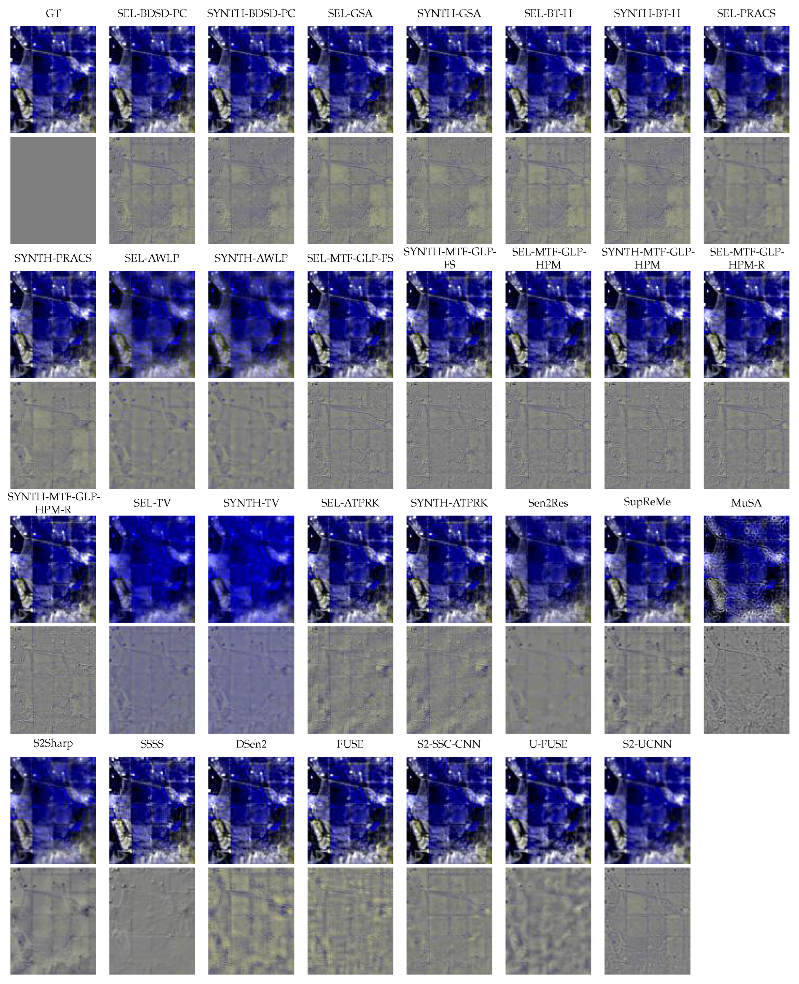
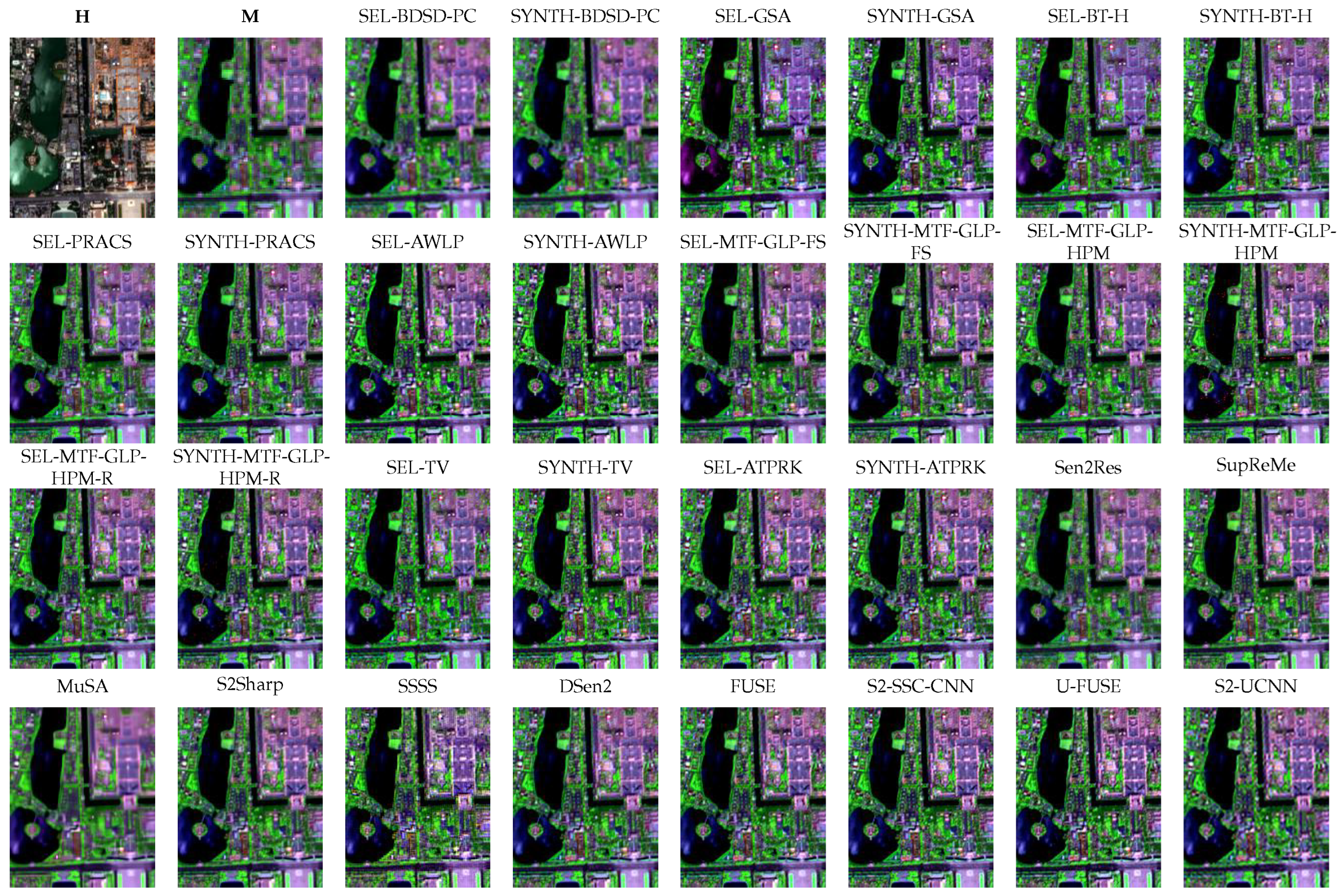
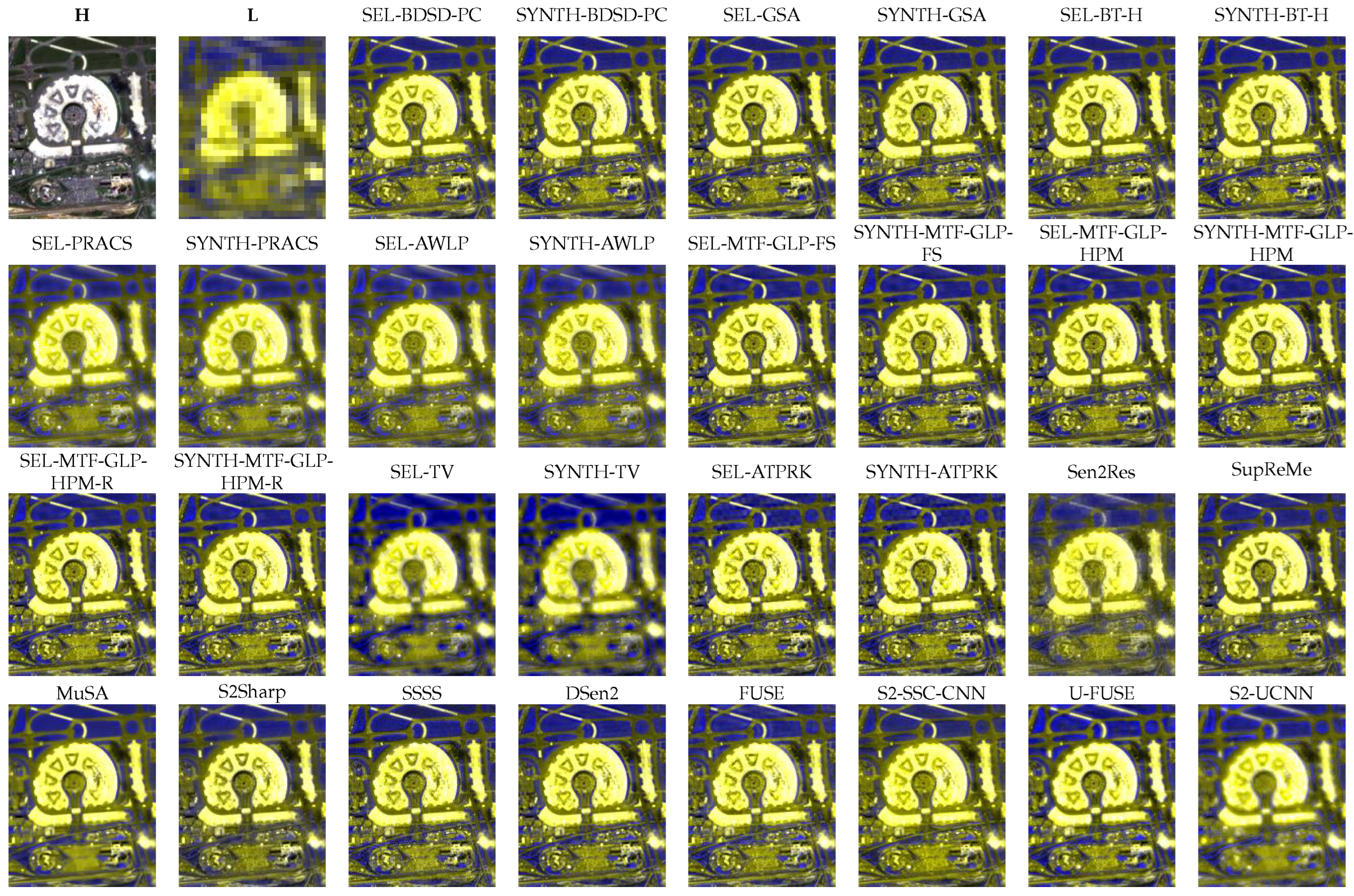
6.5. Visual Inspection

Given the large number of test images, bands, and methods, not speaking of the different evaluation contexts (RR/FR, 20/60 m), visually inspecting all the results is a rather tedious and hard task. We have selected a few meaningful (crops of) results to display, leaving the reader the possibility to explore a larger set of results on the paper GitHub (https://github.com/matciotola/Sentinel2-SR-Toolbox, accessed on 4 June 2025).

Let us start with the RR framework for which we display the (cropped) GT and the results obtained for the 20 m bands on the Brisbane image (Figure 4) and for the 60 m bands on the Reynosa image (Figure 5). In the former case, only three out of six bands are displayed in the RGB composition. In the latter case, where only two bands are concerned, the RGB visualization is obtained by replicating one of the bands. By visually inspecting these results, we can notice both spectral and spatial defects. In general, spatial artifacts are easier to detect due to the higher sensitivity of human visual perception to the mid-frequencies. On the contrary, minor color shifts are hardly noticed. For this reason, in Figure 4 and Figure 5, the error maps obtained by subtracting the GT from the pansharpened image are also provided. Sometimes, the spectral aberrations are evident. It is the case, for example, of the yellow patch visible at the center of the 20 m GT image of Figure 4, which shifts (in color) toward the green in several results (e.g., SYNTH-GSA, SHYNT-BT-H, SYNTH-PRACS). From the spatial point of view, we can notice a lack of sharpness in several results, e.g., SYNTH-BDSD-PC, Sen2Res, and MuSA. Moving to the RR 60 m results (Figure 5), spectral distortion is hard to see, whereas spatial defects such as blurring (many cases) or artifacts (MuSA) are clearly visible.

Moving to the FR framework, let us start by recalling that no GTs are available in this case; therefore, the results have to be compared with the two input components in terms of spectral or spatial consistency. These “reference” images are then displayed first on the top-left part of the figure to allow a comparison with the results. In particular, we have selected the Beijing (Figure 6) and Paris (Figure 7) images for the 20 and 60 m sets, respectively. The HR “spatial” reference is an RGB composition of three out of four 10 m bands. Instead, the other input (LR bands to super-resolve) represents the “spectral” reference. Consistent spectral distortions can be easily noticed through visual inspection, for example, SEL-GSA, MuSA, and SSSS on the 20 m set and SEL-TV, FUSE, and S2-UCNN on the 60 m set. These behaviors are actually reflected numerically in the $D_{\lambda }$ scores, a confirmation of the reliability of this index for measuring spectral quality. Furthermore, from the spatial point of view, blurring phenomena are observed for several solutions, for example, SEL-BDSD-PC on 20 m bands, SYNTH-AWLP on 60 m bands, and MuSA, SSSS, and S2-UCNN on both band sets. Overall, also in this case, we note a good coherence between the visual (spatial) judgment of the results and the related index $D_{\rho }$.

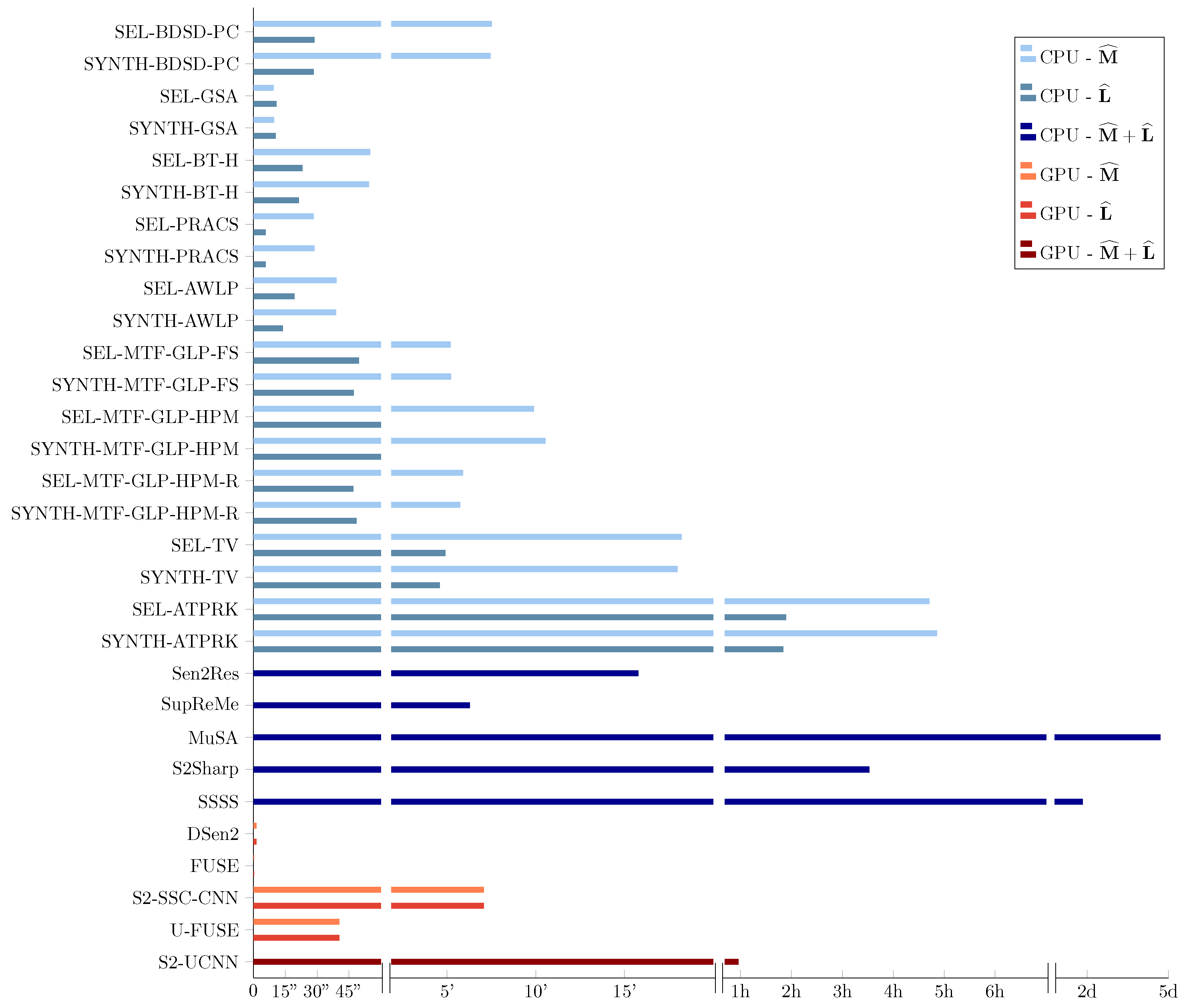
6.6. Computational Efficiency

All experiments were carried out on the same server, an NVIDIA DGX Station A100, equipped with a 64-core AMD EPYC 7742 processor, 504 GB of DDR4 RAM, and four NVIDIA A100-SXM4 GPUs with 40 GB of GDDR5 memory each. The conventional CS, MRA, and MBO methods were run on the CPU, while the DL-based methods were run on a single GPU. The average run time for each method on the 2400 × 2400 FR test images is reported in Figure 8 (pay attention to the non-uniform time scale). However, computational scalability depends on the available hardware, so we do not draw general conclusions regarding this issue. We only observe that some methods, both DL- (e.g., DSen2 and Fuse) and model-based (SEL-GSA, SYNTH-GSA, SEL-PRACS, and SYNTH-PRACS), have negligible run time, a quality to be considered in practical applications. Others are exceedingly slow, such as the CPU-based SSSS and MuSA and the GPU-based S2-UCNN.

6.7. Discussion

Keeping in mind the six evaluation properties (a)–(f), this section outlines the main strengths and weaknesses of current SoTA methods, as highlighted in this review. These aspects also reflect the key open challenges that future research is expected to address. One of the primary issues in the context of S2 sharpening is the applicability of traditional pansharpening algorithms, originally designed for MS fusion, to this more complex setting. The S2 scenario presents specific challenges, such as varying resolution ratios between $\mathbf{H}$, $\mathbf{M}$, and $\mathbf{L}$, and the almost absent spectral overlap between bands. Despite these difficulties, the results, both quantitative (see Table 3, Table 4 and Table 5) and qualitative (see Figure 4, Figure 5, Figure 6 and Figure 7), suggest that many pansharpening methods, especially those from the CS and MRA families, can still provide competitive performance compared with S2-specific sharpening techniques.

However, it is important to emphasize that no single method emerges as uniformly superior across all criteria. This fact clearly emerges from

Table 6. Summary of the strengths and weaknesses of the compared S2 sharpening methods. The evaluation follows the six properties (a)–(f) defined at the beginning of the section: (a) generalization across datasets, (b) generalization across scales, (c) sharpening performance on both $\mathbf{M}$ and $\mathbf{L}$, (d) spectral and spatial quality balance, (e) perceptual quality, and (f) computational efficiency. Symbols: ★: fair, $★★$: good, $★★★$: excellent.

		Generalization Dataset	Generalization Scales	$\mathbf{M}+\mathbf{L}$ Sharpening	Spe. & Spa. Balance	Perceptive Quality	Computational Efficiency
SEL -	BDSD-PC	$★★$	$★★$	★	$★★$	★	$★★$
SYNTH -	BDSD-PC	$★★$	$★★$	★	$★★★$	★	$★★$
SEL-	GSA	$★★$	$★★★$	$★★★$	$★★$	$★★$	$★★★$
SYNTH -	GSA	$★★$	$★★$	$★★$	$★★$	$★★$	$★★★$
SEL -	BT-H	$★★$	$★★★$	$★★★$	$★★$	★	$★★$
SYNTH -	BT-H	$★★$	$★★$	$★★$	$★★★$	$★★$	$★★$
SEL -	PRACS	$★★$	$★★$	$★★$	$★★$	$★★$	$★★$
SYNTH -	PRACS	$★★$	$★★$	$★★$	$★★$	$★★$	$★★$
SEL -	AWLP	$★★$	$★★$	$★★★$	$★★$	$★★$	$★★$
SYNTH -	AWLP	$★★$	$★★$	$★★$	$★★$	$★★★$	$★★★$
SEL -	MTF-GLP-FS	$★★★$	$★★★$	$★★$	$★★★$	$★★$	$★★$
SYNTH -	MTF-GLP-FS	$★★★$	$★★$	$★★$	$★★$	$★★$	$★★$
SEL -	MTF-GLP-HPM	$★★★$	$★★★$	$★★★$	$★★$	$★★$	$★★$
SYNTH -	MTF-GLP-HPM	$★★$	$★★$	$★★$	$★★$	$★★$	$★★$
SEL-	MTF-GLP-HPM-R	$★★★$	$★★★$	$★★$	$★★$	$★★$	$★★$
SYNTH -	MTF-GLP-HPM-R	$★★$	$★★$	$★★$	$★★$	$★★★$	$★★$
SEL -	TV	★	$★★$	$★★$	$★★$	$★★$	$★★$
SYNTH -	TV	$★★$	$★★$	$★★$	★	$★★$	$★★$
SEL -	ATPRK	$★★$	$★★$	$★★$	$★★★$	$★★$	★
SYNTH -	ATPRK	$★★$	$★★$	$★★$	$★★★$	$★★$	★
	Sen2Res	★	★	$★★$	$★★$	$★★$	$★★$
	SupReMe	$★★$	$★★$	$★★$	$★★$	$★★★$	$★★$
	MuSA	★	★	★	★	$★★$	★
	S2Sharp	★	$★★$	$★★★$	$★★$	$★★$	★
	SSSS	★	★	★	★	★	★
	DSen2	$★★$	$★★$	$★★$	$★★$	$★★★$	$★★★$
	FUSE	$★★★$	$★★$	$★★$	$★★$	$★★$	$★★★$
	S2-SSC-CNN	$★★$	★	$★★$	★	$★★$	$★★$
	U-FUSE	$★★$	$★★$	$★★$	$★★$	$★★★$	$★★$
	S2-UCNN	$★★$	★	★	★	★	$★★$

, where we have assigned (with some necessary subjectivity) ratings to all the compared methods under the six dimensions considered. DL methods, for instance, tend to show an imbalance depending on the training strategy. Supervised approaches, such as FUSE, S2-SSC-CNN, and DSen2, perform robustly in RR settings but lose competitiveness at FR. Conversely, methods like U-FUSE demonstrate stronger performance at FR, highlighting the benefit of unsupervised strategies in realistic conditions. Traditional methods based on CS, MRA, and MBO/A remain strongly influenced by the quality of the PAN synthesis process. Among them, CS and MRA techniques stand out for their robustness and good generalization across datasets and resolution levels. Finally, MBO methods, while historically among the first SoTA solutions developed for this problem, appear to struggle compared with recent advances.

Based on these insights, future research in S2 sharpening can move in several promising directions. On the one hand, pansharpening-based approaches remain valuable due to their robustness and continued methodological development. However, to fully exploit their potential, new PAN synthesis strategies must be designed to ensure both spatial consistency and generalization across diverse contexts. On the other hand, DL-based techniques still hold enormous potential. The availability of extensive, diverse datasets and rapid progress in computer vision offers a fertile ground for developing more sophisticated and high-performing models, which may significantly advance the current state of the art.

7. Conclusions

This study introduces a comprehensive benchmarking framework for S2 sharpening aimed at supporting the development and evaluation of new algorithms in an easier and more accessible manner. By analyzing the SoTA techniques in the field, a set of representative methods that reflect the most promising approaches to Sentinel-2 sharpening is identified. These methods have been carefully re-implemented and made ready for use within a unified framework. In addition, a large dataset of real multi-resolution Sentinel-2 images is designed and released, providing a reliable basis for training and testing sharpening methods. This dataset, along with the proposed protocols, ensures a consistent and fair evaluation process. By incorporating both widely used and newly proposed performance metrics, a detailed analysis of the selected methods is conducted, highlighting their strengths, limitations, and the key challenges in the field.

This work can be seen as a snapshot of the current state of Sentinel-2 sharpening research, with the goal of inspiring further advancements. By providing a framework that encompasses algorithms, metrics, and accessible tools, we want to simplify the comparison of methods, foster collaboration, and encourage the sharing of ideas and resources among researchers. Although the initiative has notable strengths, it also has limitations. The selection of methods, while representative, is not exhaustive, and some choices may reflect subjective judgment. Moreover, certain deep learning–based approaches could not be re-implemented due to the absence of publicly available code or sufficiently detailed descriptions in the literature, leaving significant opportunities for future contributions and enhancements.

This framework is meant as an open resource that can evolve through the contributions of the research community. New methods, datasets, and evaluation protocols can be integrated to address emerging challenges and expand the scope of Sentinel-2 sharpening research. By establishing a solid foundation and inviting collaboration, the work seeks to accelerate progress in this critical area of EO and promote innovative solutions for high-quality data processing.

References

1. Ienco, D.; Interdonato, R.; Gaetano, R.; Ho Tong Minh, D. Combining Sentinel-1 and Sentinel-2 Satellite Image Time Series for land cover mapping via a multi-source deep learning architecture. ISPRS J. Photogramm. Remote Sens. 2019, 158, 11–22. [Google Scholar] [CrossRef]
2. Phiri, D.; Simwanda, M.; Salekin, S.; Nyirenda, V.R.; Murayama, Y.; Ranagalage, M. Sentinel-2 Data for Land Cover/Use Mapping: A Review. Remote Sens. 2020, 12, 2291. [Google Scholar] [CrossRef]
3. Karra, K.; Kontgis, C.; Statman-Weil, Z.; Mazzariello, J.C.; Mathis, M.; Brumby, S.P. Global land use/land cover with Sentinel 2 and deep learning. In Proceedings of the 2021 IEEE International Geoscience and Remote Sensing Symposium IGARSS, Brussels, Belgium, 11–16 July 2021; pp. 4704–4707. [Google Scholar] [CrossRef]
4. Wulder, M.A.; Masek, J.G.; Cohen, W.B.; Loveland, T.R.; Woodcock, C.E. Opening the archive: How free data has enabled the science and monitoring promise of Landsat. Remote Sens. Environ. 2012, 122, 2–10. [Google Scholar] [CrossRef]
5. Khiali, L.; Ienco, D.; Teisseire, M. Object-oriented satellite image time series analysis using a graph-based representation. Ecol. Inform. 2018, 43, 52–64. [Google Scholar] [CrossRef]
6. Baselice, F.; Ferraioli, G. Unsupervised coastal line extraction from SAR images. IEEE Geosci. Remote Sens. Lett. 2013, 10, 1350–1354. [Google Scholar] [CrossRef]
7. Razzano, F.; Stasio, P.D.; Mauro, F.; Meoni, G.; Esposito, M.; Schirinzi, G.; Ullo, S.L. AI Techniques for Near Real-Time Monitoring of Contaminants in Coastal Waters on Board Future Φsat-2 Mission. IEEE J. Sel. Top. Appl. Earth Obs. Remote Sens. 2024, 17, 16755–16766. [Google Scholar] [CrossRef]
8. Roy, D.P.; Huang, H.; Boschetti, L.; Giglio, L.; Yan, L.; Zhang, H.H.; Li, Z. Landsat-8 and Sentinel-2 burned area mapping—A combined sensor multi-temporal change detection approach. Remote Sens. Environ. 2019, 231, 111254. [Google Scholar] [CrossRef]
9. de Gélis, I.; Corpetti, T.; Lefèvre, S. Change Detection Needs Change Information: Improving Deep 3-D Point Cloud Change Detection. IEEE Trans. Geosci. Remote Sens. 2024, 62, 1–10. [Google Scholar] [CrossRef]
10. Vivone, G.; Alparone, L.; Chanussot, J.; Dalla Mura, M.; Garzelli, A.; Licciardi, G.A.; Restaino, R.; Wald, L. A critical comparison among pansharpening algorithms. IEEE Trans. Geosci. Remote Sens. 2014, 53, 2565–2586. [Google Scholar] [CrossRef]
11. Vivone, G.; Dalla Mura, M.; Garzelli, A.; Restaino, R.; Scarpa, G.; Ulfarsson, M.O.; Alparone, L.; Chanussot, J. A new benchmark based on recent advances in multispectral pansharpening: Revisiting pansharpening with classical and emerging pansharpening methods. IEEE Geosci. Remote Sens. Mag. 2020, 9, 53–81. [Google Scholar] [CrossRef]
12. Deng, L.J.; Vivone, G.; Paoletti, M.E.; Scarpa, G.; He, J.; Zhang, Y.; Chanussot, J.; Plaza, A. Machine learning in pansharpening: A benchmark, from shallow to deep networks. IEEE Geosci. Remote Sens. Mag. 2022, 10, 279–315. [Google Scholar] [CrossRef]
13. Scarpa, G.; Ciotola, M. Full-resolution quality assessment for pansharpening. Remote Sens. 2022, 14, 1808. [Google Scholar] [CrossRef]
14. Wu, X.; Feng, J.; Shang, R.; Wu, J.; Zhang, X.; Jiao, L.; Gamba, P. Multi-task multi-objective evolutionary network for hyperspectral image classification and pansharpening. Inf. Fusion 2024, 108, 102383. [Google Scholar] [CrossRef]
15. Lin, C.; Wu, C.C.; Tsogt, K.; Ouyang, Y.C.; Chang, C.I. Effects of atmospheric correction and pansharpening on LULC classification accuracy using WorldView-2 imagery. Inf. Process. Agric. 2015, 2, 25–36. [Google Scholar] [CrossRef]
16. Zhao, J.; Zhong, Y.; Hu, X.; Wei, L.; Zhang, L. A robust spectral-spatial approach to identifying heterogeneous crops using remote sensing imagery with high spectral and spatial resolutions. Remote Sens. Environ. 2020, 239, 111605. [Google Scholar] [CrossRef]
17. Mazza, A.; Guarino, G.; Scarpa, G.; Yuan, Q.; Vivone, G. PM2.5 Retrieval with Sentinel-5P Data over Europe Exploiting Deep Learning. IEEE Trans. Geosci. Remote Sens. 2025, 63, 1–17. [Google Scholar] [CrossRef]
18. Ummerle, C.; Giganti, A.; Mandelli, S.; Bestagini, P.; Tubaro, S. Leveraging Land Cover Priors for Isoprene Emission Super-Resolution. Remote Sens. 2025, 17, 1715. [Google Scholar] [CrossRef]
19. Goyens, C.; Lavigne, H.; Dille, A.; Vervaeren, H. Using hyperspectral remote sensing to monitor water quality in drinking water reservoirs. Remote Sens. 2022, 14, 5607. [Google Scholar] [CrossRef]
20. Loncan, L.; De Almeida, L.B.; Bioucas-Dias, J.M.; Briottet, X.; Chanussot, J.; Dobigeon, N.; Fabre, S.; Liao, W.; Licciardi, G.A.; Simoes, M.; et al. Hyperspectral pansharpening: A review. IEEE Geosci. Remote Sens. Mag. 2015, 3, 27–46. [Google Scholar] [CrossRef]
21. Borsoi, R.A.; Imbiriba, T.; Bermudez, J.C.M.; Richard, C.; Chanussot, J.; Drumetz, L.; Tourneret, J.Y.; Zare, A.; Jutten, C. Spectral Variability in Hyperspectral Data Unmixing: A comprehensive review. IEEE Geosci. Remote Sens. Mag. 2021, 9, 223–270. [Google Scholar] [CrossRef]
22. Dobigeon, N.; Tourneret, J.Y.; Richard, C.; Bermudez, J.C.M.; McLaughlin, S.; Hero, A.O. Nonlinear Unmixing of Hyperspectral Images: Models and Algorithms. IEEE Signal Process. Mag. 2014, 31, 82–94. [Google Scholar] [CrossRef]
23. Ciotola, M.; Guarino, G.; Vivone, G.; Poggi, G.; Chanussot, J.; Plaza, A.; Scarpa, G. Hyperspectral Pansharpening: Critical review, tools, and future perspectives. IEEE Geosci. Remote Sens. Mag. 2025, 13, 311–338. [Google Scholar] [CrossRef]
24. Brodu, N. Super-resolving multiresolution images with band-independent geometry of multispectral pixels. IEEE Trans. Geosci. Remote Sens. 2017, 55, 4610–4617. [Google Scholar] [CrossRef]
25. Lanaras, C.; Bioucas-Dias, J.; Galliani, S.; Baltsavias, E.; Schindler, K. Super-resolution of Sentinel-2 images: Learning a globally applicable deep neural network. ISPRS J. Photogramm. Remote Sens. 2018, 146, 305–319. [Google Scholar] [CrossRef]
26. Wu, J.; Lin, L.; Zhang, C.; Li, T.; Cheng, X.; Nan, F. Generating Sentinel-2 all-band 10-m data by sharpening 20/60-m bands: A hierarchical fusion network. ISPRS J. Photogramm. Remote Sens. 2023, 196, 16–31. [Google Scholar] [CrossRef]
27. Selva, M.; Aiazzi, B.; Butera, F.; Chiarantini, L.; Baronti, S. Hyper-Sharpening: A First Approach on SIM-GA Data. IEEE J. Sel. Top. Appl. Earth Obs. Remote Sens. 2015, 8, 3008–3024. [Google Scholar] [CrossRef]
28. Wang, Q.; Shi, W.; Li, Z.; Atkinson, P.M. Fusion of Sentinel-2 images. Remote Sens. Environ. 2016, 187, 241–252. [Google Scholar] [CrossRef]
29. Vaiopoulos, A.; Karantzalos, K. Pansharpening on the narrow VNIR and SWIR spectral bands of Sentinel-2. Int. Arch. Photogramm. Remote Sens. Spat. Inf. Sci. 2016, 41, 723–730. [Google Scholar] [CrossRef]
30. Park, H.; Choi, J.; Park, N.; Choi, S. Sharpening the VNIR and SWIR bands of Sentinel-2A imagery through modified selected and synthesized band schemes. Remote Sens. 2017, 9, 1080. [Google Scholar] [CrossRef]
31. Lanaras, C.; Bioucas-Dias, J.; Baltsavias, E.; Schindler, K. Super-resolution of multispectral multiresolution images from a single sensor. In Proceedings of the IEEE Conference on Computer Vision and Pattern Recognition Workshops, Honolulu, HI, USA, 21–26 July 2017; pp. 20–28. [Google Scholar]
32. Paris, C.; Bioucas-Dias, J.; Bruzzone, L. A novel sharpening approach for superresolving multiresolution optical images. IEEE Trans. Geosci. Remote Sens. 2018, 57, 1545–1560. [Google Scholar] [CrossRef]
33. Lin, C.H.; Bioucas-Dias, J.M. An Explicit and Scene-Adapted Definition of Convex Self-Similarity Prior With Application to Unsupervised Sentinel-2 Super-Resolution. IEEE Trans. Geosci. Remote Sens. 2020, 58, 3352–3365. [Google Scholar] [CrossRef]
34. Krizhevsky, A.; Sutskever, I.; Hinton, G.E. Imagenet classification with deep convolutional neural networks. In Proceedings of the Advances in Neural Information Processing Systems, Lake Tahoe, NV, USA, 3–6 December 2012; pp. 1106–1114. [Google Scholar]
35. Dong, C.; Loy, C.; He, K.; Tang, X. Image Super-Resolution Using Deep Convolutional Networks. IEEE Trans. Pattern Anal. Mach. Intell. 2016, 38, 295–307. [Google Scholar] [CrossRef] [PubMed]
36. Dosovitskiy, A.; Beyer, L.; Kolesnikov, A.; Weissenborn, D.; Zhai, X.; Unterthiner, T.; Dehghani, M.; Minderer, M.; Heigold, G.; Gelly, S.; et al. An Image is Worth 16x16 Words: Transformers for Image Recognition at Scale. In Proceedings of the International Conference on Learning Representations, Virtual Event, Austria, 3–7 May 2021. [Google Scholar]
37. Deudon, M.; Kalaitzis, A.; Goytom, I.; Arefin, M.R.; Lin, Z.; Sankaran, K.; Michalski, V.; Kahou, S.E.; Cornebise, J.; Bengio, Y. HighRes-net: Recursive Fusion for Multi-Frame Super-Resolution of Satellite Imagery. arXiv 2020, arXiv:2002.06460. [Google Scholar] [CrossRef]
38. Capliez, E.; Ienco, D.; Gaetano, R.; Baghdadi, N.; Salah, A.H.; Le Goff, M.; Chouteau, F. Multisensor Temporal Unsupervised Domain Adaptation for Land Cover Mapping With Spatial Pseudo-Labeling and Adversarial Learning. IEEE Trans. Geosci. Remote Sens. 2023, 61, 1–16. [Google Scholar] [CrossRef]
39. Schmitt, M.; Ahmadi, S.A.; Xu, Y.; Taşkin, G.; Verma, U.; Sica, F.; Hänsch, R. There Are No Data Like More Data: Datasets for deep learning in Earth observation. IEEE Geosci. Remote Sens. Mag. 2023, 11, 63–97. [Google Scholar] [CrossRef]
40. Gargiulo, M.; Mazza, A.; Gaetano, R.; Ruello, G.; Scarpa, G. A CNN-Based Fusion Method for Super-Resolution of Sentinel-2 Data. In Proceedings of the IGARSS 2018—2018 IEEE International Geoscience and Remote Sensing Symposium, Valencia, Spain, 22–27 July 2018; pp. 4713–4716. [Google Scholar] [CrossRef]
41. Palsson, F.; Sveinsson, J.R.; Ulfarsson, M.O. Sentinel-2 image fusion using a deep residual network. Remote Sens. 2018, 10, 1290. [Google Scholar] [CrossRef]
42. Gargiulo, M.; Mazza, A.; Gaetano, R.; Ruello, G.; Scarpa, G. Fast super-resolution of 20 m Sentinel-2 bands using convolutional neural networks. Remote Sens. 2019, 11, 2635. [Google Scholar] [CrossRef]
43. Wu, J.; He, Z.; Hu, J. Sentinel-2 sharpening via parallel residual network. Remote Sens. 2020, 12, 279. [Google Scholar] [CrossRef]
44. Nguyen, H.V.; Ulfarsson, M.O.; Sveinsson, J.R.; Sigurdsson, J. Zero-Shot Sentinel-2 Sharpening Using a Symmetric Skipped Connection Convolutional Neural Network. In Proceedings of the IGARSS 2020—2020 IEEE International Geoscience and Remote Sensing Symposium, Waikoloa, HI, USA, 26 September–2 October 2020; pp. 613–616. [Google Scholar] [CrossRef]
45. Nguyen, H.V.; Ulfarsson, M.O.; Sveinsson, J.R. Sharpening the 20 M Bands of SENTINEL-2 Image Using an Unsupervised Convolutional Neural Network. In Proceedings of the 2021 IEEE International Geoscience and Remote Sensing Symposium IGARSS, Brussels, Belgium, 11–16 July 2021; pp. 2875–2878. [Google Scholar] [CrossRef]
46. Ciotola, M.; Ragosta, M.; Poggi, G.; Scarpa, G. A Full-Resolution Training Framework for Sentinel-2 Image Fusion. In Proceedings of the 2021 IEEE International Geoscience and Remote Sensing Symposium IGARSS, Brussels, Belgium, 11–16 July 2021; pp. 1260–1263. [Google Scholar] [CrossRef]
47. Nguyen, H.V.; Ulfarsson, M.O.; Sveinsson, J.R.; Mura, M.D. Sentinel-2 Sharpening Using a Single Unsupervised Convolutional Neural Network With MTF-Based Degradation Model. IEEE J. Sel. Top. Appl. Earth Obs. Remote Sens. 2021, 14, 6882–6896. [Google Scholar] [CrossRef]
48. Ciotola, M.; Martinelli, A.; Mazza, A.; Scarpa, G. An Adversarial Training Framework for Sentinel-2 Image Super-Resolution. In Proceedings of the IGARSS 2022—2022 IEEE International Geoscience and Remote Sensing Symposium, Kuala Lumpur, Malaysia, 17–22 July 2022; pp. 3782–3785. [Google Scholar] [CrossRef]
49. Nguyen, H.V.; Ulfarsson, M.O.; Sveinsson, J.R.; Mura, M.D. Unsupervised Sentinel-2 Image Fusion Using a Deep Unrolling Method. IEEE Geosci. Remote Sens. Lett. 2023, 20, 1–5. [Google Scholar] [CrossRef]
50. Wald, L.; Ranchin, T.; Mangolini, M. Fusion of satellite images of different spatial resolution: Assessing the quality of resulting images. Photogramm. Eng. Remote Sens. 1997, 63, 691–699. [Google Scholar]
51. Aiazzi, B.; Alparone, L.; Baronti, S.; Garzelli, A.; Selva, M. MTF-tailored multiscale fusion of high-resolution MS and Pan imagery. Photogramm. Eng. Remote Sens. 2006, 72, 591–596. [Google Scholar] [CrossRef]
52. Alparone, L.; Aiazzi, B.; Baronti, S.; Garzelli, A.; Nencini, F.; Selva, M. Multispectral and panchromatic data fusion assessment without reference. Photogramm. Eng. Remote Sens. 2008, 74, 193–200. [Google Scholar] [CrossRef]
53. Khan, M.M.; Alparone, L.; Chanussot, J. Pansharpening quality assessment using the modulation transfer functions of instruments. IEEE Trans. Geosci. Remote Sens. 2009, 47, 3880–3891. [Google Scholar] [CrossRef]
54. Aiazzi, B.; Alparone, L.; Baronti, S.; Carlà, R.; Garzelli, A.; Santurri, L. Full-scale assessment of pansharpening methods and data products. In Proceedings of the Image and Signal Processing for Remote Sensing XX, Amsterdam, The Netherlands, 22–25 September 2014; Bruzzone, L., Ed.; International Society for Optics and Photonics, SPIE: Bellingham, WA, USA, 2014; Volume 9244, p. 924402. [Google Scholar] [CrossRef]
55. Arienzo, A.; Vivone, G.; Garzelli, A.; Alparone, L.; Chanussot, J. Full-resolution quality assessment of pansharpening: Theoretical and hands-on approaches. IEEE Geosci. Remote Sens. Mag. 2022, 10, 168–201. [Google Scholar] [CrossRef]
56. Dabov, K.; Foi, A.; Katkovnik, V.; Egiazarian, K. Color image denoising via sparse 3D collaborative filtering with grouping constraint in luminance-chrominance space. In Proceedings of the 2007 IEEE International Conference on Image Processing, San Antonio, TX, USA, 16 September–19 October 2007; IEEE: Piscataway, NJ, USA, 2007; Volume 1, pp. I-313–I-316. [Google Scholar]
57. Danielyan, A.; Katkovnik, V.; Egiazarian, K. BM3D frames and variational image deblurring. IEEE Trans. Image Process. 2011, 21, 1715–1728. [Google Scholar] [CrossRef]
58. Venkatakrishnan, S.V.; Bouman, C.A.; Wohlberg, B. Plug-and-play priors for model based reconstruction. In Proceedings of the 2013 IEEE Global Conference on Signal and Information Processing, Austin, TX, USA, 3–5 December 2013; IEEE: Piscataway, NJ, USA, 2013; pp. 945–948. [Google Scholar]
59. Ulfarsson, M.O.; Palsson, F.; Dalla Mura, M.; Sveinsson, J.R. Sentinel-2 sharpening using a reduced-rank method. IEEE Trans. Geosci. Remote Sens. 2019, 57, 6408–6420. [Google Scholar] [CrossRef]
60. He, K.; Zhang, X.; Ren, S.; Sun, J. Deep residual learning for image recognition. In Proceedings of the IEEE Conference on Computer Vision and Pattern Recognition, Las Vegas, NV, USA, 27–30 June 2016; pp. 770–778. [Google Scholar]
61. Shocher, A.; Cohen, N.; Irani, M. “zero-shot” super-resolution using deep internal learning. In Proceedings of the IEEE Conference on Computer Vision and Pattern Recognition, Salt Lake City, UT, USA, 18–23 June 2018; pp. 3118–3126. [Google Scholar]
62. Luo, S.; Zhou, S.; Feng, Y.; Xie, J. Pansharpening via Unsupervised Convolutional Neural Networks. IEEE J. Sel. Top. Appl. Earth Obs. Remote Sens. 2020, 13, 4295–4310. [Google Scholar] [CrossRef]
63. Uezato, T.; Hong, D.; Yokoya, N.; He, W. Guided deep decoder: Unsupervised image pair fusion. In Proceedings of the European Conference on Computer Vision, Glasgow, UK, 23–28 August 2020; Springer: Cham, Switzerland, 2020; pp. 87–102. [Google Scholar]
64. Ciotola, M.; Poggi, G.; Scarpa, G. Unsupervised Deep Learning-Based Pansharpening With Jointly Enhanced Spectral and Spatial Fidelity. IEEE Trans. Geosci. Remote Sens. 2023, 61, 1–17. [Google Scholar] [CrossRef]
65. Ciotola, M.; Guarino, G.; Scarpa, G. An Unsupervised CNN-Based Pansharpening Framework with Spectral-Spatial Fidelity Balance. Remote Sens. 2024, 16, 3014. [Google Scholar] [CrossRef]
66. Nguyen, H.V.; Ulfarsson, M.O.; Sveinsson, J.R.; Dalla Mura, M. Deep SURE for Unsupervised Remote Sensing Image Fusion. IEEE Trans. Geosci. Remote Sens. 2022, 60, 1–13. [Google Scholar] [CrossRef]
67. Vivone, G. Robust Band-Dependent Spatial-Detail Approaches for Panchromatic Sharpening. IEEE Trans. Geosci. Remote Sens. 2019, 57, 6421–6433. [Google Scholar] [CrossRef]
68. Aiazzi, B.; Baronti, S.; Selva, M. Improving component substitution pansharpening through multivariate regression of MS+Pan data. IEEE Trans. Geosci. Remote Sens. 2007, 45, 3230–3239. [Google Scholar] [CrossRef]
69. Lolli, S.; Alparone, L.; Garzelli, A.; Vivone, G. Haze Correction for Contrast-Based Multispectral Pansharpening. IEEE Geosci. Remote Sens. Lett. 2017, 14, 2255–2259. [Google Scholar] [CrossRef]
70. Choi, J.; Yu, K.; Kim, Y. A New Adaptive Component-Substitution-Based Satellite Image Fusion by Using Partial Replacement. IEEE Trans. Geosci. Remote Sens. 2011, 49, 295–309. [Google Scholar] [CrossRef]
71. Otazu, X.; González-Audícana, M.; Fors, O.; Núñez, J. Introduction of sensor spectral response into image fusion methods. Application to wavelet-based methods. IEEE Trans. Geosci. Remote Sens. 2005, 43, 2376–2385. [Google Scholar] [CrossRef]
72. Vivone, G.; Restaino, R.; Chanussot, J. Full Scale Regression-Based Injection Coefficients for Panchromatic Sharpening. IEEE Trans. Image Process. 2018, 27, 3418–3431. [Google Scholar] [CrossRef]
73. Alparone, L.; Garzelli, A.; Vivone, G. Intersensor Statistical Matching for Pansharpening: Theoretical Issues and Practical Solutions. IEEE Trans. Geosci. Remote Sens. 2017, 55, 4682–4695. [Google Scholar] [CrossRef]
74. Vivone, G.; Restaino, R.; Chanussot, J. A regression-based high-pass modulation pansharpening approach. IEEE Trans. Geosci. Remote Sens. 2017, 56, 984–996. [Google Scholar] [CrossRef]
75. Palsson, F.; Sveinsson, J.R.; Ulfarsson, M.O. A New Pansharpening Algorithm Based on Total Variation. IEEE Geosci. Remote Sens. Lett. 2014, 11, 318–322. [Google Scholar] [CrossRef]
76. Clerc, S.; M.P.C. Team. S2 MPC-Data Quality Report, S2-PDGS-MPC-DQR. Available online: https://sentiwiki.copernicus.eu/__attachments/1673423/S2-PDGS-MPC-DQR%20-%20S2%20MPC%20L1C%20DQR%20January%202015%20-%2001.pdf?inst-v=f9683405-accc-4a3f-a58f-01c9c5213fb1 (accessed on 25 May 2025).
77. Tu, T.M.; Su, S.C.; Shyu, H.C.; Huang, P.S. A new look at IHS-like image fusion methods. Inf. Fusion 2001, 2, 177–186. [Google Scholar] [CrossRef]
78. Garzelli, A.; Nencini, F.; Capobianco, L. Optimal MMSE pan sharpening of very high resolution multispectral images. IEEE Trans. Geosci. Remote Sens. 2008, 46, 228–236. [Google Scholar] [CrossRef]
79. Laben, C.A.; Brower, B.V. Process for Enhancing the Spatial Resolution of Multispectral Imagery Using Pan-Sharpening. U.S. Patent # 6,011,875, 4 January 2000. [Google Scholar]
80. Gillespie, A.R.; Kahle, A.B.; Walker, R.E. Color enhancement of highly correlated images. II. Channel ratio and “chromaticity” transformation techniques. Remote Sens. Environ. 1987, 22, 343–365. [Google Scholar] [CrossRef]
81. Baronti, S.; Aiazzi, B.; Selva, M.; Garzelli, A.; Alparone, L. A Theoretical Analysis of the Effects of Aliasing and Misregistration on Pansharpened Imagery. IEEE J. Sel. Top. Signal Process. 2011, 5, 446–453. [Google Scholar] [CrossRef]
82. Thomas, C.; Ranchin, T.; Wald, L.; Chanussot, J. Synthesis of Multispectral Images to High Spatial Resolution: A Critical Review of Fusion Methods Based on Remote Sensing Physics. IEEE Trans. Geosci. Remote Sens. 2008, 46, 1301–1312. [Google Scholar] [CrossRef]
83. Vivone, G.; Restaino, R.; Dalla Mura, M.; Licciardi, G.; Chanussot, J. Contrast and error-based fusion schemes for multispectral image pansharpening. IEEE Geosci. Remote Sens. Lett. 2013, 11, 930–934. [Google Scholar] [CrossRef]
84. Vivone, G.; Restaino, R.; Licciardi, G.; Dalla Mura, M.; Chanussot, J. MultiResolution Analysis and Component Substitution Techniques for Hyperspectral Pansharpening. In Proceedings of the 2014 IEEE Geoscience and Remote Sensing Symposium, Quebec City, QC, Canada, 13–18 July 2014; pp. 2649–2652. [Google Scholar]
85. Vicinanza, M.R.; Restaino, R.; Vivone, G.; Mura, M.D.; Chanussot, J. A Pansharpening Method Based on the Sparse Representation of Injected Details. IEEE Geosci. Remote Sens. Lett. 2015, 12, 180–184. [Google Scholar] [CrossRef]
86. Wei, Q.; Dobigeon, N.; Tourneret, J.Y. Fast fusion of multi-band images based on solving a Sylvester equation. IEEE Trans. Image Process. 2015, 24, 4109–4121. [Google Scholar] [CrossRef]
87. Wei, Q.; Bioucas-Dias, J.; Dobigeon, N.; Tourneret, J.Y. Hyperspectral and multispectral image fusion based on a sparse representation. IEEE Trans. Geosci. Remote Sens. 2015, 53, 3658–3668. [Google Scholar] [CrossRef]
88. Wang, Q.; Shi, W.; Atkinson, P.M.; Zhao, Y. Downscaling MODIS images with area-to-point regression kriging. Remote Sens. Environ. 2015, 166, 191–204. [Google Scholar] [CrossRef]
89. Keshava, N.; Mustard, J.F. Spectral unmixing. IEEE Signal Process. Mag. 2002, 19, 44–57. [Google Scholar] [CrossRef]
90. Armannsson, S.E.; Ulfarsson, M.O.; Sigurdsson, J.; Nguyen, H.V.; Sveinsson, J.R. A comparison of optimized Sentinel-2 super-resolution methods using Wald’s protocol and Bayesian optimization. Remote Sens. 2021, 13, 2192. [Google Scholar] [CrossRef]
91. Afonso, M.V.; Bioucas-Dias, J.M.; Figueiredo, M.A. Fast image recovery using variable splitting and constrained optimization. IEEE Trans. Image Process. 2010, 19, 2345–2356. [Google Scholar] [CrossRef]
92. Afonso, M.V.; Bioucas-Dias, J.M.; Figueiredo, M.A. An augmented Lagrangian approach to the constrained optimization formulation of imaging inverse problems. IEEE Trans. Image Process. 2010, 20, 681–695. [Google Scholar] [CrossRef] [PubMed]
93. Masi, G.; Cozzolino, D.; Verdoliva, L.; Scarpa, G. Pansharpening by Convolutional Neural Networks. Remote Sens. 2016, 8, 594. [Google Scholar] [CrossRef]
94. Lim, B.; Son, S.; Kim, H.; Nah, S.; Mu Lee, K. Enhanced deep residual networks for single image super-resolution. In Proceedings of the IEEE Conference on Computer Vision and Pattern Recognition Workshops, Honolulu, HI, USA, 21–26 July 2017; pp. 136–144. [Google Scholar]
95. Yang, J.; Fu, X.; Hu, Y.; Huang, Y.; Ding, X.; Paisley, J. PanNet: A Deep Network Architecture for Pan-Sharpening. In Proceedings of the 2017 IEEE International Conference on Computer Vision (ICCV), Venice, Italy, 22–29 October 2017. [Google Scholar] [CrossRef]
96. Scarpa, G.; Vitale, S.; Cozzolino, D. Target-Adaptive CNN-Based Pansharpening. IEEE Trans. Geosci. Remote Sens. 2018, 56, 5443–5457. [Google Scholar] [CrossRef]
97. Jiang, Y.; Ding, X.; Zeng, D.; Huang, Y.; Paisley, J. Pan-sharpening with a hyper-Laplacian penalty. In Proceedings of the IEEE International Conference on Computer Vision, Santiago, Chile, 7–13 December 2015; pp. 540–548. [Google Scholar]
98. Ronneberger, O.; Fischer, P.; Brox, T. U-net: Convolutional networks for biomedical image segmentation. In Proceedings of the Medical Image Computing and Computer-Assisted Intervention–MICCAI 2015: 18th International Conference, Munich, Germany, 5–9 October 2015; Proceedings, Part III. Springer: Cham, Switzerland, 2015; pp. 234–241. [Google Scholar]
99. Ciotola, M.; Vitale, S.; Mazza, A.; Poggi, G.; Scarpa, G. Pansharpening by Convolutional Neural Networks in the Full Resolution Framework. IEEE Trans. Geosci. Remote Sens. 2022, 60, 1–17. [Google Scholar] [CrossRef]
100. Ulyanov, D.; Vedaldi, A.; Lempitsky, V. Deep image prior. In Proceedings of the IEEE Conference on Computer Vision and Pattern Recognition, Salt Lake City, UT, USA, 18–23 June 2018; pp. 9446–9454. [Google Scholar]
101. Heckel, R.; Hand, P. Deep decoder: Concise image representations from untrained non-convolutional networks. arXiv 2018, arXiv:1810.03982. [Google Scholar]
102. Salgueiro, L.; Marcello, J.; Vilaplana, V. Single-Image Super-Resolution of Sentinel-2 Low Resolution Bands with Residual Dense Convolutional Neural Networks. Remote Sens. 2021, 13, 5007. [Google Scholar] [CrossRef]
103. Wang, X.; Yu, K.; Wu, S.; Gu, J.; Liu, Y.; Dong, C.; Qiao, Y.; Change Loy, C. ESRGAN: Enhanced Super-Resolution Generative Adversarial Networks. In Proceedings of the European Conference on Computer Vision (ECCV) Workshops, Munich, Germany, 8–14 September 2018. [Google Scholar]
104. Stein, C.M. Estimation of the mean of a multivariate normal distribution. Ann. Stat. 1981, 9, 1135–1151. [Google Scholar] [CrossRef]
105. Solo, V. A sure-fired way to choose smoothing parameters in ill-conditioned inverse problems. In Proceedings of the 3rd IEEE International Conference on Image Processing, Lausanne, Switzerland, 19 September 1996; IEEE: Piscataway, NJ, USA, 1996; Volume 3, pp. 89–92. [Google Scholar]
106. Boyd, S.; Parikh, N.; Chu, E.; Peleato, B.; Eckstein, J. Distributed Optimization and Statistical Learning via the Alternating Direction Method of Multipliers. Found. Trends® Mach. Learn. 2011, 3, 1–122. [Google Scholar] [CrossRef]
107. Vasilescu, V.; Datcu, M.; Faur, D. A CNN-Based Sentinel-2 Image Super-Resolution Method Using Multiobjective Training. IEEE Trans. Geosci. Remote Sens. 2023, 61, 1–14. [Google Scholar] [CrossRef]
108. Armannsson, S.E.; Ulfarsson, M.O.; Sigurdsson, J. A Learned Reduced-Rank Sharpening Method for Multiresolution Satellite Imagery. Remote Sens. 2025, 17, 432. [Google Scholar] [CrossRef]
109. Vivone, G.; Dalla Mura, M.; Garzelli, A.; Pacifici, F. A benchmarking protocol for pansharpening: Dataset, preprocessing, and quality assessment. IEEE J. Sel. Top. Appl. Earth Obs. Remote Sens. 2021, 14, 6102–6118. [Google Scholar] [CrossRef]
110. Vivone, G.; Garzelli, A.; Xu, Y.; Liao, W.; Chanussot, J. Panchromatic and Hyperspectral Image Fusion: Outcome of the 2022 WHISPERS Hyperspectral Pansharpening Challenge. IEEE J. Sel. Top. Appl. Earth Obs Remote Sens. 2023, 16, 166–179. [Google Scholar] [CrossRef]
111. Wald, L. Data Fusion: Definitions and Architectures—Fusion of Images of Different Spatial Resolutions; Les Presses de l’École des Mines: Paris, France, 2002. [Google Scholar]
112. Yuhas, R.H.; Goetz, A.F.H.; Boardman, J.W. Discrimination among semi-arid landscape endmembers using the Spectral Angle Mapper (SAM) algorithm. In Proceedings of the Summaries of the 3rd Annual JPL Airborne Geoscience Workshop, Pasadena, CA, USA, 1–5 June 1992; pp. 147–149. [Google Scholar]
113. Garzelli, A.; Nencini, F. Hypercomplex quality assessment of multi/hyperspectral images. IEEE Trans. Geosci. Remote Sens. 2009, 6, 662–665. [Google Scholar] [CrossRef]
114. Wang, Z.; Bovik, A.C. A universal image quality index. IEEE Signal Process. Lett. 2002, 9, 81–84. [Google Scholar] [CrossRef]
115. Alparone, L.; Garzelli, A.; Vivone, G. Spatial Consistency for Full-Scale Assessment of Pansharpening. In Proceedings of the IGARSS 2018—2018 IEEE International Geoscience and Remote Sensing Symposium, Valencia, Spain, 22–27 July 2018; pp. 5132–5134. [Google Scholar] [CrossRef]
Figure 1. Spectral coverage of MS, HS (colored bars), and PAN (gray bar) sensors across various remote sensing satellites. The resolutions (in meters) at which each sensor operates are shown on the left. The names of the satellites are shown on the right.
Remotesensing 17 01983 g001
Figure 2. RGB representation of the 15 S2 test crops used for benchmarking. Bands B04 (Red), B03 (Green), and B02 (Blue) were selected to create the composite. Quantile-based histogram stretching was applied for enhanced visualization. The images are arranged by content, ranging from natural landscapes to agricultural areas and urban environments.
Remotesensing 17 01983 g002
Figure 3. Locations of S2 tiles used for training, validation, and testing. Red, grey, and white dots represent training, validation, and test zones, respectively.
Remotesensing 17 01983 g003
Figure 4. Sentinel-2 20 m bands sharpening results (cropped to 145 × 180 pixels) for Brisbane at RR. The GT image (B11, B8A, B5) and sharpening results (top row) with error map (bottom row).
Remotesensing 17 01983 g004
Figure 5. Sentinel-2 60 m bands sharpening results (cropped to 145 × 180 pixels) for Reynosa at RR. The GT image (B1, B1, B9) and sharpening results (top row) with error map (bottom row).
Remotesensing 17 01983 g005
Figure 6. Sentinel-2 20 m bands sharpening results (cropped to 145 × 180 pixels) for Beijing at FR. The H image (B2, B3, B4) and the M component (B11, B8A, B5), upsampled using nearest-neighbor interpolation, are followed by the corresponding sharpening results for each method.
Remotesensing 17 01983 g006
Figure 7. Sentinel-2 60 m bands sharpening results (cropped to 145 × 180 pixels) for Paris at FR. The H image (B2, B3, B4) and the L component (B1, B1, B9), upsampled using nearest-neighbor interpolation, are followed by the corresponding sharpening results for each method.
Remotesensing 17 01983 g007
Figure 8. Average running time, reported in seconds, minutes, hours, and days, per 2400 × 2400 image (FR test images) at inference. DL methods are run on GPU, and the remaining ones on CPU.
Remotesensing 17 01983 g008