Abstract
Hyperspectral image classification (HSIC) represents a significant area of research within the domain of remote sensing. Given the intricate nature of hyperspectral images and the substantial volume of data they generate, it is essential to introduce innovative methodologies to effectively address the data pre-processing challenges encountered in HSIC. In this paper, we draw inspiration from the Segment Anything Model (SAM) within the realm of large language models to propose its application for HSIC, aiming to achieve significant advancements and breakthroughs in this field. Initially, we constructed the SAM and labeled a limited number of samples as segmentation prompts for the model. We conducted HSIC experiments utilizing three publicly available hyperspectral image datasets: Indian Pines (IP), Salinas (SA), and Pavia University (PU). Furthermore, a voting strategy was implemented during these experiments, with only five samples selected from each land type. The classification results obtained from the SAM-based hyperspectral images were compared with those derived from eight distinct machine learning, deep learning, and Transformer models. The findings indicate that the SAM requires only a limited number of samples to effectively perform hyperspectral image classification, achieving higher accuracy than the other models discussed in this paper. Building on this foundation, a voting strategy was implemented, leading to significant enhancements in the overall accuracy (OA) of HSIC across three datasets. The improvements were quantified at 66.76%, 74.66%, and 70.53%, respectively, culminating in final accuracies of 80.29%, 90.66%, and 86.51%. In this study, the SAM is utilized for unsupervised classification, thereby reducing the need for sample labeling while attaining effective classification outcomes.
1. Introduction
Hyperspectral image contains rich spectral spatial information that can elucidate the response characteristics of ground objects across various spectra [1]. HSIC has been extensively applied to a range of earth science tasks, including environmental mapping [2], climate change studies [3], agricultural management [4,5], mineral exploration [6], and geological research [7]. HSIC represents a critical aspect of hyperspectral image processing and analysis. Hyperspectral images, which encompass hundreds of bands, are transformed into classification maps through pixel-by-pixel category labeling. These classification maps provide an intuitive representation of the distribution of ground objects within the image by employing distinct colors for different types of ground features [8,9]. Early approaches to HSIC primarily focused on extracting spectral information while neglecting spatial data. Commonly utilized feature classifiers include Random Forest (RF) [10], Support Vector Machine (SVM) [11], and K-Nearest Neighbor (KNN) [12]. Moreover, researchers have proposed several methods tailored for spectral dimensionality reduction and information extraction from hyperspectral images. These methods include principal component analysis (PCA) [13], independent component analysis (ICA) [14], and linear discriminant analysis (LDA) [15]. By calculating spectral correlation information along the spectral dimension of hyperspectral images, these techniques can effectively reduce data dimensionality while extracting relevant spectral features. However, the drawback of this approach lies in its difficulty to comprehensively capture nonlinear relationships and intricate spectral characteristics, which can easily lead to information loss or suboptimal dimensionality reduction. Additionally, the design of manual features necessitates in-depth expertise, thereby increasing complexity and introducing subjective influences that may compromise the stability and reliability of classification outcomes.
In recent years, numerous efforts have been made to classify hyperspectral images using deep learning techniques [16]. The convolutional neural network (CNN) model is among the most widely utilized deep learning architectures for HSIC. CNNs employ multiple convolutional, activation, and pooling layers for feature extraction and are typically followed by fully connected layers and softmax classifiers. For hyperspectral images, CNNs can be employed to extract either spectral or spatial features based on the input provided to the network. Hu et al. [17] designed a one-dimensional CNN model that utilizes the spectral information inherent in hyperspectral images as input, effectively extracting spectral dimensional convolutional features. Building upon this foundation, Zhao et al. [18] implemented a 2D-CNN to extract spatial features from local cubes of data. Wang et al. [19] proposed a hybrid HSIC model that leverages the initial few convolutional layers to capture position-invariant mid-layer features before employing a recurrent layer to extract contextual details related to the spectrum. To enhance computational efficiency, Liu et al. [20] introduced an improved CNN architecture aimed at mitigating overfitting issues while enhancing generalization capabilities through the use of 1×1 convolutional kernels. Gao et al. [21] incorporated a global average pooling layer into their design to reduce training parameters within the network while facilitating higher-dimensional feature extraction. Subsequent methodologies increasingly focus on integrating both spatial and spectral features. For example, Ran et al. [22] proposed an enhanced pixel-pair feature (PPF) method that extracts pixel pairs exhibiting spatial adjacency relationships from hyperspectral images as distinctive features. Zhong et al. [23] introduced a supervised spectral–spatial residual network (SSRN) specifically designed for feature extraction in hyperspectral imagery; this approach employs a series of three-dimensional convolutions within their respective spectral residual blocks and spatial residual blocks. Roy et al. [24] integrated the features of 2D and 3D CNNs to develop a hierarchical convolutional network model, termed HybridSN, which effectively extracts spatial–spectral features while reducing computational complexity and enhancing classification accuracy. To account for variations in the spatial environment across different hyperspectral image blocks, Li et al. [25] employed adaptive weight learning instead of fixed weights, thereby introducing greater spatial detail. Deep networks are crucial for capturing global features within an image; however, traditional convolution methods often fall short in modeling long-range correlations. Furthermore, convolutional networks necessitate a substantial amount of annotated data to effectively learn feature representations. As a result, when confronted with small sample tasks that possess limited annotated data, the accuracy of image classification tends to be low due to inadequate model training.
The successful implementation of these methodologies hinges on a critical prerequisite: each category must possess a sufficient number of samples, a requirement that is both costly and impractical in hyperspectral remote sensing tasks. Consequently, achieving effective classification with limited training sets has emerged as an urgent necessity within this field. In response to this challenge, researchers have made persistent efforts to enhance classification performance under the conditions of small training datasets. Zhang et al. [26] proposed a locally balanced embedding algorithm designed to extract spectral dimension features while thoroughly considering both spatial and spectral characteristics; this approach addresses the issue posed by the scarcity of labeled samples. Liu et al. [27] trained their model by simulating scenarios typical of small sample classifications during the training phase, aiming to extract features characterized by reduced intra-class distances and increased inter-class distances, thereby improving classification accuracy for small sample sizes. Ma et al. [28] developed a two-stage relation learning network that leverages other hyperspectral images for general information sharing while also allowing fine-tuning on specific hyperspectral images for targeted information acquisition. Then, several new feature learning structures have emerged, with the most prominent being the attention mechanism proposed in natural language processing (NLP) [29]. This mechanism has proven to be more effective at integrating global features at an early stage. The performance of classification models is enhanced by incorporating an attention module into the architecture. Fu et al. [30] introduced a HSIC framework based on class-level band learning, which not only improved the model’s sensitivity to class-specific information within spectral bands but also significantly increased classification accuracy through the joint extraction of multi-scale spatial features and global spectral features. Xue et al. [31] proposed a novel hierarchical residual network that employs the attention mechanism to assign adaptive weights to spatial and spectral features across different scales. This approach enables the extraction of multi-scale spatial and spectral features at a granular level, thereby expanding the receptive field range and enhancing the model’s feature representation capabilities. Building upon this foundation, the self-attention mechanism facilitates deeper global understanding and contextual analysis through interactive learning among internal elements. In contrast to traditional convolutional neural networks (CNNs), self-attention mechanisms establish connections between any two locations within an image while maintaining a global receptive field. This allows for the more comprehensive capturing of complex patterns and information dependencies present in images. Leveraging this self-attention mechanism, Hong et al. [32] introduced SpectralFormer, which is a backbone network capable of learning local spectral sequence information from adjacent strips to generate grouped spectral embeddings applicable to both pixel- and patch-based inputs. To optimize feature extraction processes more effectively, some researchers have explored various types of attention mechanisms in hyperspectral classification tasks. Among them, Ma et al. [33] integrated the convolutional block attention module (CBAM) [34], a widely utilized tool in computer vision, into the feature learning process of hyperspectral images, thereby proposing an innovative double-branch multi-attention (DBMA) network. To address the limitations of these methods in spectral feature extraction, Zhang et al. [35] introduced a hierarchical self-attention network (HSAN) which constructs a hierarchical self-attention module for feature learning, designs a hierarchical fusion mode, and leverages the self-attention mechanism within the transformer structure to capture context information. This approach minimizes the loss of effective information during feature learning and enhances the integration of features across different levels.
While the attention mechanism effectively promotes global interaction between contexts in hyperspectral image classification (HSIC), challenges remain in terms of generalization. Especially for large and diverse hyperspectral datasets, the generalizability of the model emerges as a critical challenge. The emergence of large-scale models offers valuable insights for hyperspectral image classification (HSIC). Large language models (LLMs), renowned for their robust capabilities in understanding, generating, and processing vast amounts of textual data, have achieved significant success in natural language processing (NLP) tasks. The Segment Anything Model (SAM) [36], an exemplary application of LLMs in visual tasks, has extended the frontiers of image segmentation. After extensive training with substantial datasets, the SAM has demonstrated its versatility across various domains, particularly in remote sensing applications. Ren et al. [37] conducted a comprehensive evaluation of the SAM’s performance on several remote sensing segmentation datasets, including Solar [38], Inria [39], DeepGlobe and DeepGlobe Roads [40], 38-Cloud [41], and Parcel Delineation [42]. Their findings indicate that the SAM achieves comparable performance to supervised models in segmenting certain ground objects, showcasing strong generalizability. Based on its fundamental components—namely, a large-scale pre-trained visual encoder, a flexible prompting mechanism (which includes point, box, or text prompts), and a lightweight mask decoder—the SAM effectively extracts common visual features through the encoder. It utilizes prompt information to guide the decoder in dynamically adapting to various targets, thereby achieving efficient feature interaction and semantic segmentation. In traditional small sample classification of hyperspectral images, convolutional neural networks often suffer from overfitting and inadequate feature extraction due to their inherent model complexity and limitations in local receptive fields. Although transformers are capable of capturing long-range dependencies, they require substantial amounts of data and entail high computational costs, which constrains their effectiveness in scenarios with limited sample sizes. In this paper, we introduce the SAM’s prompt driving mechanism into the task of hyperspectral small sample classification. The optimization of spectrum–space feature fusion is achieved through the integration of pre-trained prior knowledge and interactive prompts. Compared to traditional methods, our model significantly reduces reliance on labeled data, effectively balancing the relationship between local details and global context, even with a limited number of samples. This approach enhances both classification accuracy and generalization capabilities. This study utilizes publicly available datasets from IP, SA, and PU for experimentation. In these experiments, only five labeled samples per land type are selected as cue information for the SAM, thereby successfully implementing SAM-based HSIC.
2. Materials and Methods
2.1. SAM Structure and Composition
The SAM comprises three components: an image encoder, a prompt encoder, and a mask decoder. The architecture of the model is illustrated in Figure 1.
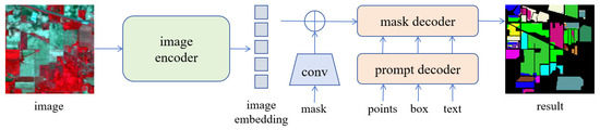
Figure 1.
Structure of the SAM.
2.1.1. Image Encoder
The image encoder is implemented using the vision transformer (ViT) [43] backbone network and pre-trained with mask strategies from the mask automatic encoder (MAE) [44]. It is designed to embed the input tensor, enabling subsequent integration with manual prompts. The ViT architecture encompasses three models, ViT-B, ViT-L, and ViT-H, each offering distinct trade-offs between computational requirements and model performance. The primary differences among these models lie in the number of layers and parameters, as detailed in Table 1. Increasing the number of layers and parameters significantly enhances the model’s ability to capture complex features of the input image, albeit at the cost of higher computational demands.

Table 1.
Three ViT models of SAM.
The image encoder utilizes the custom PyTorch2.0.0 module ImageEncoderViT to implement the image encoding component of the vision transformer, transforming and modeling the embeddings of image patches. Each transformer encoder layer comprises a multi-head self-attention mechanism, a feed-forward network, and residual connections. By leveraging the ViT model, the self-attention mechanism captures global image information, thereby enhancing the model’s ability to understand and represent images. The architecture of the image encoder is illustrated in Figure 2.
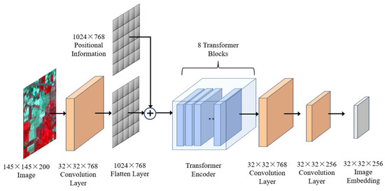
Figure 2.
Structure of the image encoder.
The standard transformer accepts a one-dimensional (1D) token embedding a sequence as the input. To process two-dimensional (2D) images, the image is transformed into , where (H, W) represents the dimensions of the original image, C denotes the number of channels, (P, P) is the resolution of each patch, and N is the number of patches, which serves as the effective input sequence length for the transformer. The transformer processes all its layers with a constant hidden dimension D. y represents the image, and prior to training and fine-tuning, the classification heads are connected to z0, as shown in Equation (1). The classification head is implemented using a multi-layer perceptron (MLP) with a hidden layer for pre-training and a single linear layer for fine-tuning. The resulting sequence of embedding vectors serves as input to the encoder. The transformer encoder comprises multi-head self-attention (MSA) and MLP blocks, as described in Equations (2) and (3). Layer normalization (LN) is applied before each block, and residual connections are added after each block, as detailed in Equation (4).
Hyperspectral images require preprocessing prior to being input into the image encoder. The original data are represented in dimensions of H × W × B, where H and W denote the spatial dimensions corresponding to H × W pixels, and each pixel encompasses B spectral bands. The default image encoder developed by the SAM is specifically designed to process three-channel RGB images. To accommodate this requirement, principal component analysis (PCA) is employed to reduce the dimensionality of hyperspectral data. In the practical implementation, the three-dimensional hyperspectral cube is initially reshaped into a two-dimensional matrix (number of pixels × number of bands). Subsequently, the first three principal components are extracted using PCA, effectively compressing the B-dimensional spectral information of each pixel into three dimensions. The normalized principal components are then mapped to a range of 0–255 in order to generate a pseudo-RGB image.
The pre-processed pseudo-RGB images are subsequently input into the SAM’s image encoder module, utilizing a pre-trained vit_h model. As the image traverses through the encoder, it is initially segmented into 16 × 16 image blocks, each of which is transformed into an embedded vector via linear projection. Following the processing through multiple layers of transformer blocks, a final image embedding with a spatial hierarchical structure is produced, resulting in dimensions of 256 × 64 × 64. This procedure effectively converts the original H × W pixel image into a dense vector representation that encapsulates rich semantic features, thereby providing essential feature support for subsequent segmentation tasks.
2.1.2. Prompt Encoder
The prompt encoder module supports sparse feature points, bounding boxes, text, and dense feature masks. The SAM segmentation mask decoder integrates the embedded prompt information with the image encoding features to generate the final segmentation output. The SAM can segment objects by including or excluding them through simple clicks or interactive point selection. Additionally, the SAM can generate multiple valid masks when there is uncertainty in identifying the objects to be segmented. It can also automatically identify and generate masks for all objects present in the image. Immediately after the pre-processed image is embedded, the SAM can provide a segmentation mask for any query, enabling real-time interaction with the model. The architecture of the prompt encoder is illustrated in Figure 3. Its role is to map the prompts into feature space for the mask decoder to produce the final segmentation result. It processes two types of prompts: sparse prompts (dots, boxes, text) and dense prompts (masks). In this study, the mask input serves as a dense prompt, and convolutional processing is employed. The size of the prompt embedding is first reduced via downsampling before being input into the prompt encoder, and then it is matched to the size of the image embedding using three layers of 2D convolution.
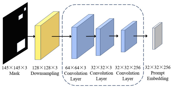
Figure 3.
Structure of the prompt encoder.
In the context of prompt generation, the primary objective is to construct interactive prompts utilizing ground truth annotation data derived from hyperspectral imagery. For each target category, five spatial coordinate points are randomly sampled from the corresponding region as positive samples, while points are sampled from regions associated with other categories to serve as negative samples. These coordinate points, along with their respective positive and negative labels, are transformed into embedded representations by the prompt encoder. It is recommended that the encoder employs an embedding space shared with the image encoder to convert two-dimensional coordinate position information into high-dimensional vectors through positional encoding. Additionally, it maps both positive and negative labels to directional features. This processing facilitates a unified interaction between spatial position information and semantic relationships with image features.
2.1.3. Mask Decoder
The primary function of the mask decoder is to perform object segmentation by predicting masks for the input image. To enhance performance, the mask decoder employs several advanced techniques, including the transformer architecture, upsampling layers, hypernetworks, and a mask quality prediction head. First, the module utilizes the transformer architecture to process the input feature maps, extracting contextual information for each location in the image. By learning effective feature representations, the transformer helps the model better capture the position and shape of objects during mask prediction. Next, an upsampling layer is applied to the output feature map from the transformer to restore the resolution to match that of the original image. This step preserves more detail and enables the model to generate masks with higher accuracy. Hypernetwork technology is integrated into the SAM to dynamically generate network weights. The mask decoder leverages the hypernetwork to adaptively adjust the model parameters, enhancing its flexibility and adaptability to various input scenarios. This capability is particularly beneficial for hyperspectral image segmentation across different contexts. Finally, the mask quality prediction head evaluates the quality of the generated masks. By assessing the degree of match between the predicted masks and the ground truth labels, this component facilitates the model’s learning of more accurate mask representations, thereby improving the overall accuracy of hyperspectral image segmentation. Multimodal feature fusion is implemented within the mask decoder module. This module receives the hyperspectral image embedding from the image encoder and the cue embedding from the cue encoder, facilitating feature interaction through a cross-attention mechanism. During the decoding process, dynamically generated convolutional kernels are applied to image feature maps of varying scales, progressively upsampling to produce multi-resolution segmentation masks. The model only outputs the optimal single mask prediction, which enhances prediction stability and simplifies post-processing in scenarios with limited sample sizes. The mask probability values for each pixel are processed using a threshold to generate binary segmentation results.
2.2. SAM Fusion Improvement Strategy
The SAM is an unsupervised classification model capable of prompt-based segmentation, achieving zero-shot image segmentation without the need for additional training data or fine-tuning. Instead of traditional prompt encoders, the SAM introduces an auxiliary network known as the injection network to provide necessary category information. The primary role of the injection network is to transfer knowledge from previously trained models to the SAM, thereby enriching its representational capabilities. The injection network comprises multiple MLP blocks, each consisting of two fully connected layers and a nonlinear activation function. These MLP blocks are designed with a flat structure to balance model complexity and expressiveness. During training, the injection network transfers internal knowledge by integrating with other components of the SAM. Specifically, the output of the injection network serves as a feature map that is concatenated or summed with other features to enhance the diversity and richness of the feature representation. In this manner, the injection network facilitates an unsupervised learning mechanism for the SAM, enabling it to leverage internal knowledge and cues from the dataset for task-specific learning.
To ensure the validity of the SAM classification, a voting strategy has been implemented during the classification process. This procedure is illustrated in Figure 4. The foundation of the voting strategy is based on a multi-projection integration approach. The spectral bands of hyperspectral data are segmented into 10 continuous sub-bands, with each sub-band group independently subjected to principal component analysis (PCA) to produce 10 sets of pseudo-RGB images. Each set of pseudo-RGB images subsequently generates an independent classification result following inference by the SAM. Specifically, for each sub-band projection image, the model outputs a classification mask of size H × W that corresponds to the spatial dimensions of the original hyperspectral data, indicating pixel category predictions for that particular projection. For every pixel, we tally the number of times it is predicted to belong to each category across all projections and select the category with the highest vote count as its final classification. The advantage of this voting strategy lies in its ability to effectively reduce errors that may arise from relying on a single projection. Given that the spectral characteristics inherent in hyperspectral data can vary significantly across different bands, a solitary projection may not adequately capture all discriminative features present within the data.
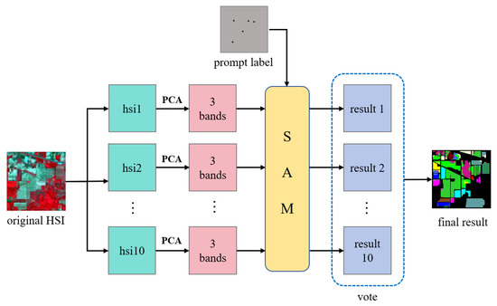
Figure 4.
Flowchart of the SAM fusion improvement strategy.
3. Experiments and Results
3.1. Experimental Data and Evaluation Indicators
To validate the effectiveness of the proposed method, three publicly available hyperspectral image datasets from Indian Pines (IP), Salinas (SA), and Pavia University (PU) were selected for experimentation. Among these datasets, IP and SA represent agricultural scenarios, whereas PU represents a more complex urban scenario. The detailed information regarding the datasets is provided in Table 2.
Table 2.
Detailed information regarding the dataset.
The overall accuracy (OA), average accuracy (AA), and kappa coefficient were employed as evaluation metrics for the classification performance of different methods. The same set of tests was repeated 10 times, and the average value was taken as the final test result.
- OAThe formula for calculating OA is provided in Equation (5).where TP represents the number of samples that are actually true and correctly predicted as true. TN represents the number of samples that are actually false and correctly predicted as false. FP represents the number of samples that are actually false but incorrectly predicted as true. FN represents the number of samples that are actually true but incorrectly predicted as false.
- AAThe calculation formula for AA is provided in Equation (6).where TPi represents the TP count for class i, FNi represents the FN count for class i, and n denotes the total number of categories across all features.
- Kappa coefficientThe formula for calculating the kappa coefficient is provided in Equation (7).where Po is equivalent to the OA, Pe is provided by Equation (8), and N represents the total number of test samples as given by Equation (9).N = TP + TN + FP + FN
3.2. Experiments and Results
To verify the accuracy of SAM-based HSIC under small sample conditions, three representative hyperspectral datasets, IP, SA, and PU, were utilized for image classification experiments. For each land type, labeled samples were selected as a priori knowledge samples. The experimental results demonstrate that the SAM can efficiently classify hyperspectral images from different scenes. The experiment was repeated 10 times using the same sample combination, and the average of the results from these 10 trials was calculated to verify the stability and reliability of the model through consistent experimental outcomes.
To assess the effectiveness of the method proposed in this paper, five labeled samples were randomly selected as supervised samples for each category of ground objects across three datasets. Eight distinct methods—SVM, 1D-CNN, 2D-CNN, 3D-CNN, SSRN, HybridSN, DFSL, and transformer—were employed for HSIC. The classification results obtained from these methods were compared with those derived from SAM-based HSIC to evaluate the performance of the SAM in ground object classification. The findings are presented in Figure 5, Figure 6 and Figure 7, as well as in Table 3, Table 4 and Table 5.
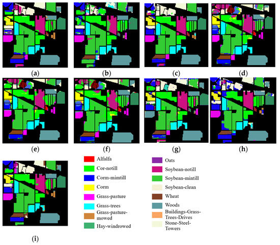
Figure 5.
Classification results of various methods applied to the IP dataset. (a) SAM; (b) SVM; (c) 1D-CNN; (d) 2D-CNN; (e) 3D-CNN; (f) SSRN; (g) HybridSN; (h) DFSL; (i) transformer.
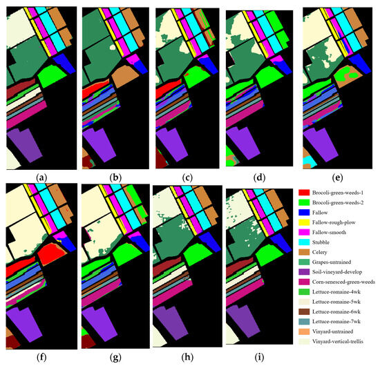
Figure 6.
Classification outcomes of various methodologies applied to the SA dataset. (a) SAM; (b) SVM; (c) 1D-CNN; (d) 2D-CNN; (e) 3D-CNN; (f) SSRN; (g) HybridSN; (h) DFSL; (i) transformer.
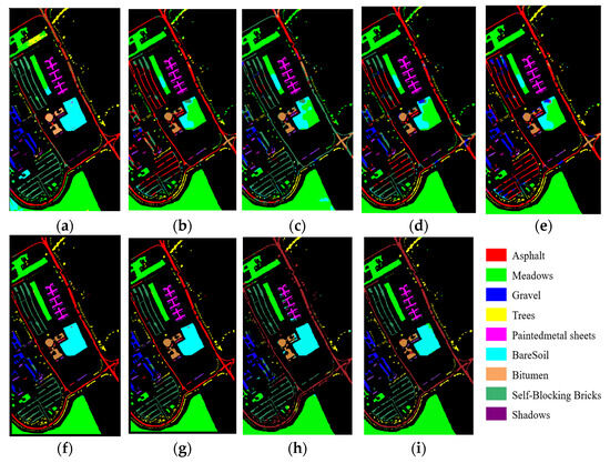
Figure 7.
Results of various classification methods applied to the PU dataset. (a) SAM; (b) SVM; (c) 1D-CNN; (d) 2D-CNN; (e) 3D-CNN; (f) SSRN; (g) HybridSN; (h) DFSL; (i) transformer.
Table 3.
Classification performance of SAM, SVM, 1D-CNN, 2D-CNN, 3D-CNN, SSRN, HybridSN, DFSL, and transformer on the IP dataset.
Table 4.
Classification results of SAM, SVM, 1D-CNN, 2D-CNN, 3D-CNN, SSRN, HybridSN, DFSL and transformer on SA dataset.
Table 5.
Classification performance of SAM, SVM, 1D-CNN, 2D-CNN, 3D-CNN, SSRN, HybridSN, DFSL, and transformer on the PU dataset.
The experimental results presented in Figure 5, Figure 6 and Figure 7, as well as in Table 3, Table 4 and Table 5, demonstrate that the application of the SAM method across three datasets—IP, SA, and PU—yields satisfactory classification outcomes with only five samples selected for each land type. The overall classification accuracies achieved by the SAM for these three datasets are recorded at 80.29%, 90.66%, and 86.51%, respectively; these figures significantly surpass the classification results obtained from the other eight methods discussed in this paper. This confirms that the SAM is capable of performing HSIC effectively with a minimal number of prior samples. Furthermore, it illustrates that the SAM possesses the adaptability to tackle new tasks without any prior examples while still achieving high levels of classification accuracy without necessitating pre-training.
As illustrated in Figure 5 and Table 3, the classification performance of the SAM is relatively low for the IP dataset. This may be attributed to the high number of categories and complex features present within the IP dataset, which necessitates a greater volume of samples for more effective classification. The intricate characteristics of ground objects contribute to increased diversity among the samples in this dataset, with each category exhibiting unique spectral traits that must be accurately identified and distinguished by the model. As the number of categories increases, the feature differences between various categories within the dataset may also become increasingly subtle and complex. Consequently, models are required to possess enhanced expressiveness and discriminative capabilities to effectively capture these nuances across different categories. As a result, classifying such complex features becomes more challenging, leading to a decline in overall classification performance.
3.3. Analysis of PCA Contribution Rate
To quantitatively assess the information retention efficiency of principal component analysis (PCA) during the dimensionality reduction process of hyperspectral data, a statistical analysis was conducted on the PCA contribution rates and cumulative contribution rates for the IP, SA, and PU datasets. According to the voting strategy, the bands from each dataset were randomly divided into ten groups. Each group underwent independent PCA processing, resulting in the extraction of three principal components: PC1, PC2, and PC3. To provide a comprehensive illustration of the contribution rates of the three principal components, we calculated both the average contribution rate and the cumulative contribution rate across ten experimental groups. The “average contribution rate” reflects the mean explanatory power of each principal component across all groups, while the “average cumulative contribution rate” indicates the overall extent to which data features are represented by the first three principal components. These metrics were subsequently employed as representative indicators for this dataset, with the results presented in Table 6.
Table 6.
PCA average contribution rate and average cumulative contribution rate.
Table 6 presents the experimental results, indicating that the average contribution rate of PC1 in the IP dataset is 89.46%. Furthermore, the average cumulative contribution rate of the first three principal components rises to 96.65%. For SA and PU, the average contribution rates of PC1 are notably higher, reaching 98.40% and 98.13%, respectively. Additionally, it is worth noting that only the average cumulative contribution rates of the first two principal components have achieved levels of 99.86% (PU) and 99.72% (SA). This result indicates that, in the context of the designed 10-group band division, the first three principal components retained through PCA dimensionality reduction effectively capture over 95% of the variance information present in the original data. Furthermore, the average contribution rate of higher-order principal components (such as PC3) is less than 1.61%, suggesting that their complementary effect on overall variance is exceedingly limited.
This result delineates the threshold of potential information loss during dimensionality reduction. While three-dimensional compression may overlook certain higher-order spectral details, the fundamental spectral features are effectively captured by the first two principal components. Furthermore, the averaging across multiple experiments reinforces the statistical significance of this conclusion. The high and stable cumulative contribution rate indicates that the low-dimensional space resulting from dimensionality reduction effectively preserves the core features of the original hyperspectral data, while minimizing information loss. Furthermore, it is demonstrated that the integration of band grouping with PCA dimensionality reduction strikes an effective balance between model compatibility (in RGB format) and information integrity, thereby providing a robust framework for SAM-based hyperspectral image classification.
3.4. The Influence of the Quantity of Labeled Samples on the Results
To evaluate the performance of the SAM under small sample conditions, systematic experiments were conducted on three classical hyperspectral datasets from Indian Pines, Salinas and Pavia University. The classification accuracy of the SAM under different sample numbers was analyzed by gradually increasing the number of labeled samples from 1 to 15 with an interval of 2. The results are shown in Table 7, Table 8 and Table 9, in which the optimal results of each type of accuracy index are marked in bold.
Table 7.
Classification accuracy of different sample numbers based on IP datasets.
Table 8.
Classification accuracy of different sample numbers based on SA datasets.
Table 9.
Classification accuracy of different sample numbers based on PU datasets.
From Table 7, Table 8 and Table 9, it is evident that the SAM method demonstrates significant advantages under small sample conditions, particularly when the sample size is limited to five. Furthermore, it maintains a commendable classification capability even in scenarios with very low sample sizes. Specifically, when each category comprises only five samples, the overall accuracy (OA) of the SAM achieved values of 80.29%, 90.66%, and 86.51% for the IP, SA, and PU datasets, respectively. These results indicate that a sample size of five effectively balances the adequacy of labeling information with noise control; this approach not only provides sufficient spectral feature identification data, but also mitigates redundancy or category confusion that may arise from an excessive number of samples.
Taking the PU dataset as an example, when the sample size increased from one to five, the overall accuracy (OA) surged from 33.54% to 86.51%, and the Kappa coefficient rose from 19.95 to 82.05. This demonstrates the SAM’s capability to rapidly extract essential spectral features even with extremely limited annotations. The performance of the IP dataset further corroborates this conclusion: with a sample size of five, the OA increases by 36 percentage points compared to using just one sample; however, when the sample size is further expanded to 15 samples, there is a slight decline in OA to 75.92%. This suggests that the model may be sensitive to local noise or shifts in data distribution. It is noteworthy that performance variations across different datasets are closely linked to spectral separability. Due to significant spectral differences among categories, only three samples are required for the SA dataset to approach performance saturation, whereas five samples are necessary for both IP and PU datasets in order to overcome performance bottlenecks caused by high spectral overlap. This disparity underscores a design advantage of SAM cue encoders: through a space-spectral joint attention mechanism, the model can dynamically concentrate on discriminative bands derived from limited annotations, thereby alleviating issues related to spectral redundancy.
3.5. Ablation Experiments
To thoroughly evaluate the effectiveness of the SAM for HSIC, ablation experiments were conducted utilizing the IP, SA, and PU datasets with various band combinations. Ten distinct groups of slices, each containing different spectral information, were extracted from the original 3D hyperspectral image. Principal component analysis (PCA) was employed to reduce the spectral dimensionality to three components. Subsequently, ten different classification results were generated using the SAM. The final classification result was obtained through a voting strategy. The specific outcomes are presented in Table 10.
Table 10.
Results of OA with and without the implementation of a voting strategy.
By comparing the classification results obtained with and without the voting strategy, we can verify the effectiveness of this approach in enhancing the hyperspectral image classification performance of the SAM. As illustrated in Table 10, for the IP, SA, and PU datasets, the overall classification accuracy (OA) improved by 0.91%, 2.09%, and 5.75%, respectively, following the implementation of the voting strategy. This enhancement is primarily attributed to the optimization and integration of multiple groups of classification results derived from different band combinations through the voting mechanism. Specifically, the original hyperspectral image is partitioned into ten subsets based on varying band combinations; each subset yields independent classification results after PCA reduction. The category with the highest frequency among these results is selected as the final output via a voting process. This method effectively harnesses and integrates the distinctive advantages offered by various band combinations while significantly increasing kappa coefficient by 7.65 percentage points within the PU dataset. Moreover, simultaneous improvements in average accuracy (AA) further substantiate that voting strategy provides balanced enhancements across different categories’ classification performance. This experiment demonstrates that by amalgamating classification outcomes from multiple band combinations, a voting strategy can effectively mitigate errors arising from any single projection, thereby improving the overall performance in SAM-based hyperspectral image classifications.
3.6. Computational Efficiency Analysis
To assess the computational efficiency of the proposed method, we selected transformer, DFSL, HybridSN, and SSRN—methods that demonstrate strong overall performance in comparison to others—for comparative analysis against SAM. The results of this analysis are presented in Table 11, Table 12 and Table 13. The experiments were conducted on a PC equipped with an Intel (R) Core (TM) i7-14650HX processor running at 2.20 GHz, an NVIDIA GeForce RTX 4060 GPU graphics card with 8 GB of GPU memory and 32 GB of RAM.
Table 11.
Computing efficiency based on IP datasets.
Table 12.
Computing efficiency based on SA datasets.
Table 13.
Computing efficiency based on PU datasets.
By comparing the computational efficiency of the Spectral Angle Mapper (SAM) with several mainstream hyperspectral classification models, it is evident from Table 11, Table 12 and Table 13 that SAM demonstrates a particularly high level of time efficiency. From a model architecture perspective, this efficiency can be attributed to the deep adaptation of its pre-training features. As a foundational model for pre-training based on large-scale datasets, the SAM significantly mitigates the training overhead associated with hyperspectral classification tasks by employing lightweight parameter fine-tuning strategies. On the PU dataset, the SAM’s training time was a mere 12.52 s—an impressive advantage stemming from the knowledge transfer capabilities of its pre-trained weights, which circumvent the extensive iterative calculations typically required when training a model from scratch. Furthermore, the test time for classification using the SAM remains consistently stable at approximately 8–9 s, representing a reduction of over 50% compared to traditional methods.
The time efficiency advantage of the SAM is synergistic with its multi-projection integration strategy. Although this approach increases the computational load associated with data preprocessing due to 10 sets of independent projections, the SAM’s inference flow effectively maintains the time cost of multi-projection inference within a reasonable range by leveraging shared image encoder features and a batch processing mechanism. Experimental results indicate that the total time cost for the SAM on the PU dataset is 34.17% lower than that of the second-best method, DFSL, demonstrating the SAM’s robustness in complex processing workflows. In addition, the SAM’s cue encoder facilitates the efficient adaptation of hyperspectral data through lightweight modifications. Traditional interactive segmentation models often encounter computational bottlenecks when processing high-dimensional spectral information; however, the SAM alleviates this issue by compressing the computational load of cue encoding into an acceptable range through a spectral-sensitive attention mechanism and a parameter-sharing strategy. This design empowers the model to respond swiftly to user prompts while maintaining stable reasoning speed in scenarios with limited samples.
4. Conclusions
In order to better leverage the global features of hyperspectral images and enhance the generalization capabilities of HSIC models, this paper introduces the application of the SAM within a large language model for HSIC. Three public datasets—IP, SA, and PU—were utilized to conduct HSIC experiments. In these experiments, only five samples were selected for each land type as segmentation prompt information for SAM. Additionally, a voting strategy was implemented to improve classification accuracy and meet the high precision requirements inherent in HSIC applications.
- (1)
- The comparison of classification results across the eight methods reveals that the SAM exhibits a robust zero-sample learning capability. It requires only a limited number of samples to effectively accomplish hyperspectral image classification tasks. Furthermore, the overall accuracy achieved in hyperspectral image classification using the SAM is significantly superior to that of the eight models evaluated.
- (2)
- The implementation of the voting strategy significantly enhances the overall accuracy of the HSIC. This indicates that the integration of the voting strategy with the SAM can effectively leverage the advantages offered by features from different spectral resolutions in their respective classifications.
However, in hyperspectral images characterized by a high number of categories and intricate features—particularly when addressing subtle variations in spectral characteristics—the performance of SAM-based HSIC may be somewhat compromised. Therefore, for such complex datasets, optimization can be achieved by enhancing the attention mechanism to bolster the model’s capacity to focus on key features. Additionally, improvements can be made in feature extraction methods, classification algorithms, and optimization techniques. Increasing the training data and refining the model architecture are also essential steps to meet the high accuracy requirements for HSIC.
Author Contributions
Conceptualization, K.M. and B.L.; methodology, B.L. and C.Y.; validation, C.Y.; formal analysis, Q.H. and S.L.; investigation, S.L. and P.H.; data curation, J.H.; writing—original draft preparation, C.Y.; writing—review and editing, K.M. and B.L.; visualization, J.H.; supervision, P.H.; project administration, B.L. and Q.H.; funding acquisition, Q.H. All authors have read and agreed to the published version of the manuscript.
Funding
This research was supported by the National Natural Science Foundation of China (No. 42401501), National Key Research and Development Program of China (No. 2024YFC3212200) and the Henan Science Foundation for Distinguished Young Scholars of China (No. 242300421041).
Data Availability Statement
The original contributions presented in the study are included in the article, further inquiries can be directed to the corresponding author.
Acknowledgments
The authors would like to thank the website for providing the data used in the paper and the reviewers for their insightful comments.
Conflicts of Interest
The authors declare no conflicts of interest.
References
- Du, P.J.; Xia, J.S.; Xue, Z.H.; Tan, K.; Su, H.J.; Bao, R. Review of Hyperspectral Remote Sensing Image Classification. J. Remote Sens. 2016, 20, 236–256. [Google Scholar]
- Chen, L.F.; Zhang, Y.; Zou, M.M.; Xu, Q.; Li, L.J.; Li, X.Y.; Tao, J.H. Overview of Atmospheric CO2 Remote Sensing from Space. J. Remote Sens. 2015, 19, 1–11. [Google Scholar]
- Wang, G.; Yuan, S.; Ye, S. Retrieval of Atmospheric Three-Dimensional Wind Field Based on Hyperspectral GIRS Infrared Brightness Temperature. Infrared 2023, 44, 39–45. [Google Scholar]
- Huang, Y.J.; Tian, Y.C.; Zhang, Q. Estimation of Aboveground Biomass of Mangroves in Maowei Sea of Beibu Gulf Based on ZY-1-02D Satellite Hyperspectral Data. Spectrosc. Spectr. Anal. 2023, 43, 3906–3915. [Google Scholar]
- Xia, C.Z.; Jiang, Y.Y.; Zhang, Y.X. Estimation of Soil Organic Matter in Maize Field of Black Soil Area Based on UAV Hyperspectral Image. Spectrosc. Spectr. Anal. 2023, 43, 2617–2626. [Google Scholar]
- Wang, Y.J. Research Progress and Prospect on Ecological Disturbance Monitoring in Mining Area. Acta Geod. Cartogr. Sin. 2017, 46, 1705–1716. [Google Scholar]
- Li, N.; Dong, X.F.; Gan, F.P.; Yan, B.K. Application Evaluation of ZY-1-02D Satellite Hyperspectral Data in Geological Survey. Spacecr. Eng. 2020, 29, 186–191. [Google Scholar]
- Anand, R.; Veni, S.; Aravinth, J. Big Data Challenges in Airborne Hyperspectral Image for Urban Landuse Classification. In Proceedings of the 2017 International Conference on Advances in Computing, Communications and Informatics (ICACCI), Delhi, India, 13–16 September 2017; pp. 1808–1814. [Google Scholar]
- Yu, X.C.; Liu, B.; Xue, Z.X. Potential Analysis and Prospect of Hyperspectral Ground Object Recognition. Acta Geod. Cartogr. Sin. 2023, 52, 1115–1125. [Google Scholar]
- Ham, J.; Chen, Y.; Crawford, M.M. Investigation of the Random Forest Framework for Classification of Hyperspectral Data. IEEE Trans. Geosci. Remote Sens. 2005, 43, 492–501. [Google Scholar] [CrossRef]
- Camps-Valls, G.; Bruzzone, L. Kernel-Based Methods for Hyperspectral Image Classification. IEEE Trans. Geosci. Remote Sens. 2005, 43, 1351–1362. [Google Scholar] [CrossRef]
- Ma, L.; Crawford, M.M.; Tian, J. Local Manifold Learning-Based K-Nearest-Neighbor for Hyperspectral Image Classification. IEEE Trans. Geosci. Remote Sens. 2010, 48, 4099–4109. [Google Scholar] [CrossRef]
- Prasad, S.; Bruce, L.M. Limitations of Principal Components Analysis for Hyperspectral Target Recognition. IEEE Geosci. Remote Sens. 2008, 5, 625–629. [Google Scholar] [CrossRef]
- Villa, A.; Benediktsson, J.A.; Chanussot, J. Hyperspectral Image Classification with Independent Component Discriminant Analysis. IEEE Trans. Geosci. Remote Sens. 2011, 49, 4865–4876. [Google Scholar] [CrossRef]
- Bandos, T.V.; Bruzzone, L.; Camps-Valls, G. Classification of Hyperspectral Images with Regularized Linear Discriminant Analysis. IEEE Trans. Geosci. Remote Sens. 2009, 47, 862–873. [Google Scholar] [CrossRef]
- Pu, S.L. Research on Deep Learning Models for Hyperspectral Image Classification. Acta Geod. Cartogr. Sin. 2023, 52, 172. [Google Scholar]
- Hu, W.; Huang, Y.Y.; Wei, L. Deep Convolutional Neural Networks for Hyperspectral Image Classification. J. Sens. 2015, 2015, 258619. [Google Scholar] [CrossRef]
- Zhao, W.Z.; Du, S.H. Spectral-Spatial Feature Extraction for Hyperspectral Image Classification: A Dimension Reduction and Deep Learning Approach. IEEE Trans. Geosci. Remote Sens. 2016, 54, 4544–4554. [Google Scholar] [CrossRef]
- Wang, K.X.; Zheng, S.Y.; Li, R.; Gui, L. A Deep Double-Channel Dense Network for Hyperspectral Image Classification. J. Geod. 2021, 4, 46–62. [Google Scholar]
- Liu, X.; Deng, C.W.; Chanussot, J. StfNet: A Two-Stream Convolutional Neural Network for Spatiotemporal Image Fusion. IEEE Trans. Geosci. Remote Sens. 2019, 57, 6552–6564. [Google Scholar] [CrossRef]
- Roy, S.K.; Krishna, G.; Dubey, S.R. HybridSN: Exploring 3-D–2-D CNN Feature Hierarchy for Hyperspectral Image Classification. IEEE Trans. Geosci. Remote Sens. 2019, 17, 277–281. [Google Scholar] [CrossRef]
- Gao, H.M.; Yang, Y.; Li, C.M. Joint Alternate Small Convolution and Feature Reuse for Hyperspectral Image Classification. ISPRS Int. J. Geo-Inf. 2018, 7, 349. [Google Scholar] [CrossRef]
- Ran, L.Y.; Zhang, Y.N.; Wei, W. A Hyperspectral Image Classification Framework with Spatial Pixel Pair Features. Sensors 2017, 17, 2421. [Google Scholar] [CrossRef]
- Zhong, Z.L.; Li, J.; Luo, Z.; Chapman, M. Spectral-Spatial Residual Network for Hyperspectral Image Classification: A 3D Deep Learning Framework. IEEE Trans. Geosci. Remote Sens. 2017, 56, 847–858. [Google Scholar] [CrossRef]
- Li, S.M.; Zhu, X.Y.; Liu, Y. Adaptive Spatial-Spectral Feature Learning for Hyperspectral Image Classification. IEEE Access 2019, 7, 61534–61547. [Google Scholar] [CrossRef]
- Zhang, H.; Li, Y.; Zhang, Y. Spectral-spatial classification of hyperspectral imagery using a dual-channel convolutional neural network. Remote Sens. Lett. 2017, 8, 438–447. [Google Scholar] [CrossRef]
- Liu, B.; Yu, X.C.; Yu, A.Z. Deep Few-Shot Learning for Hyperspectral Image Classification. IEEE Trans. Geosci. Remote Sens. 2019, 4, 2290–2304. [Google Scholar] [CrossRef]
- Ma, X.; Ji, S.; Wang, J.; Geng, J.; Wang, H. Hyperspectral image classification based on two-phase relation learning network. IEEE Trans. Geosci. Remote Sens. 2019, 12, 10398–10409. [Google Scholar] [CrossRef]
- Vaswani, A.; Shazeer, N.; Parmar, N.; Uszkoreit, J.; Jones, L.; Gomez, A.N.; Kaiser, Ł.; Polosukhin, I. Attention is All You Need. In Proceedings of Neural Information Processing Systems; NIPS: Long Beach, CA, USA, 2017; pp. 5998–6008. [Google Scholar]
- Fu, Y.; Liu, H.; Zou, Y.; Wang, S.; Li, Z.; Zheng, D. Category-Level Band Learning-Based Feature Extraction for Hyperspectral Image Classification. IEEE Trans. Geosci. Remote Sens. 2024, 62, 5503916. [Google Scholar] [CrossRef]
- Xue, Z.; Yu, X.; Liu, B. HResNetAM: Hierarchical Residual Network with Attention Mechanism for Hyperspectral Image Classification. IEEE J.-Sel. Top. Appl. Earth Obs. Remote Sens. 2021, 14, 3566–3580. [Google Scholar] [CrossRef]
- Hong, D.F.; Han, Z.; Yao, J. Spectralformer: Rethinking Hyperspectral Image Classification with Transformers. IEEE Trans. Geosci. Remote Sens. 2021, 60, 5518615. [Google Scholar] [CrossRef]
- Ma, W.P.; Yang, Q.F.; Wu, Y. Double-branch multi-attention mechanism network for hyperspectral image classification. Remote Sens. 2019, 11, 1307. [Google Scholar] [CrossRef]
- Woo, S.; Park, J.; Lee, J.Y. Cbam: Convolutional block attention module. In Proceedings of the 2018 European Conference on Computer Vision, Munich, Germany, 8–14 September 2018; Springer: Cham, Switzerland, 2018; pp. 3–19. [Google Scholar]
- Zhang, Y.C.; Zheng, X.T.; Lu, X.Q. Hyperspectral Image Classification Method Based on Hierarchical Transformer Network. Acta Geod. Cartogr. Sin. 2023, 52, 1139–1147. [Google Scholar]
- Kirillov, A.; Mintun, E.; Ravi, N.; Mao, H.; Rolland, C.; Gustafson, L.; Xiao, T.; Whitehead, S.; Berg, A.C.; Lo, W.Y.; et al. Segment Anything. In Proceedings of the IEEE/CVF International Conference on Computer Vision (ICCV), Paris, France, 1–6 October 2023; pp. 4015–4026. [Google Scholar]
- Ren, S.; Luzi, F.; Lahrichi, S.; Kassaw, K.; Collins, L.M.; Bradbury, K.; Malof, J.M. Segment Anything, from Space? In Proceedings of the IEEE/CVF Winter Conference on Applications of Computer Vision, Waikoloa, HI, USA, 1–6 January 2024; pp. 8340–8350. [Google Scholar]
- Bradbury, K.; Saboo, R.; L Johnson, T.; Malof, J.M.; Devarajan, A.; Zhang, W.; Collins, L.M.; G. Newell, R. Distributed Solar Photovoltaic Array Location and Extent Dataset for Remote Sensing Object Identification. Sci. Data 2016, 3, 160106. [Google Scholar] [CrossRef] [PubMed]
- Maggiori, E.; Tarabalka, Y.; Charpiat, G.; Alliez, P. Can Semantic Labeling Methods Generalize to Any City? The Inria Aerial Image Labeling Benchmark. In Proceedings of the 2017 IEEE International Geoscience and Remote Sensing Symposium (IGARSS), Fort Worth, TX, USA, 23–28 July 2017; pp. 3226–3229. [Google Scholar]
- Demir, I.; Koperski, K.; Lindenbaum, D.; Pang, G.; Huang, J.; Basu, S.; Hughes, F.; Tuia, D.; Raskar, R. DeepGlobe 2018: A Challenge to Parse the Earth through Satellite Images. In Proceedings of the IEEE Conference on Computer Vision and Pattern Recognition Workshops (CVPRW), Salt Lake City, UT, USA, 18–22 June 2018; pp. 172–181. [Google Scholar]
- Mohajerani, S.; Saeedi, P. Cloud-Net: An End-to-End Cloud Detection Algorithm for Landsat 8 Imagery. In Proceedings of the 2019 IEEE International Geoscience and Remote Sensing Symposium (IGARSS), Yokohama, Japan, 28 July–2 August 2019; pp. 1029–1032. [Google Scholar]
- Aung, H.L.; Uzkent, B.; Burke, M.; Lobell, D.; Ermon, S. Farm Parcel Delineation Using Spatio-Temporal Convolutional Networks. In Proceedings of the IEEE/CVF Conference on Computer Vision and Pattern Recognition Workshops (CVPRW), Seattle, WA, USA, 14–19 June 2020; pp. 76–77. [Google Scholar]
- Dosovitskiy, A.; Beyer, L.; Kolesnikov, A.; Weissenborn, D.; Zhai, X.; Unterthiner, T.; Dehghani, M.; Minderer, M.; Heigold, G.; Gelly, S.; et al. An Image is Worth 16 × 16 Words: Transformers for Image Recognition at Scale. In Proceedings of the Ninth International Conference on Learning Representations, Virtual, 3–7 May 2021. [Google Scholar]
- He, K.; Chen, X.; Xie, S.; Li, Y.; Dollár, P.; Girshick, R. Masked Autoencoders are Scalable Vision Learners. In Proceedings of the IEEE/CVF Conference on Computer Vision and Pattern Recognition (CVPR), New Orleans, LA, USA, 18–24 June 2022; pp. 16000–16009. [Google Scholar]
Disclaimer/Publisher’s Note: The statements, opinions and data contained in all publications are solely those of the individual author(s) and contributor(s) and not of MDPI and/or the editor(s). MDPI and/or the editor(s) disclaim responsibility for any injury to people or property resulting from any ideas, methods, instructions or products referred to in the content. |
© 2025 by the authors. Licensee MDPI, Basel, Switzerland. This article is an open access article distributed under the terms and conditions of the Creative Commons Attribution (CC BY) license (https://creativecommons.org/licenses/by/4.0/).