Time Series Analysis of Vegetation Recovery After the Taum Sauk Dam Failure

Abstract

On 14 December 2005, there was a catastrophic flood after a failure in the upper reservoir at the Taum Sauk Plant in southern Missouri. While there has been extensive research on the cause of the dam’s failure and the flood’s immediate impact, there has been limited investigation on how vegetation in and around the resulting flood scour has changed since this event. This study fills this gap through a time-series analysis using imagery sourced from GloVis and Planet Explorer to quantify vegetation levels prior to the flood (2005) through to 2024. Vegetation level was calculated using the Normalized Difference Vegetation Index (NDVI), which measures the level of greenness via light reflected by vegetation. Vegetation levels inside of the scour were compared to two 120 m buffer areas surrounding the scour, immediately adjacent (0–120 m) and at 120–240 m from the scour’s edge. Within the scour, NDVI analysis showed a dramatic loss of vegetation immediately after the flood, followed by varying levels for several years, before a steady increase in the proportion of areas with vegetation starting in 2014. The buffer area adjacent to the edge of the scour showed a similar pattern, but at lower magnitudes of change, which likely reflects the ragged edge created by the flood. The buffer area farther from the edge showed a consistent pattern of high vegetation, which likely reflects the broader landscape. While ground truthing confirmed these patterns between 2006 and 2011, in 2012, the ground truthing revealed much recovery in small local areas within the scour that were not apparent though NDVI analysis. These local areas of recovery were reflected in the pattern of recolonization of the scour from nearby glades (i.e., natural habitats of exposed bedrock) by glade flora and by the eastern collared lizard (Crotaphytus collaris collaris), an apex predator adapted to living in rocky, open areas and a bioindicator of vegetation recovery. While recovery of vegetation occurred steadily after 2012, ground truthing indicated that the original oak/hickory forest was now a minor component of this recovery, and that glade species dominated the former forested area.

1. Introduction

Between 1960 and 1963, the Taum Sauk pumped-storage hydroelectric plant, located on Proffit Mountain in southeast Missouri (Figure 1), was constructed to generate electricity by the overnight pumping of water from a lower reservoir, formed by damming the East Fork of the Black River, into an upper reservoir on the mountain top, and then releasing this water back into the lower reservoir to generate electricity during peak power periods [1,2]. The upper reservoir was constructed without a spillway, making monitoring of water level imperative [3]. While a large quantity of water was observed overtopping the northwest portion of the upper reservoir on 25 September 2005 [1,2], repairs of loose sensors at the bottom of the upper reservoir were postponed pending other scheduled maintenance to avoid additional shutdowns of the plant [2]. Unfortunately, at 5 AM on 14 December 2005, the high-water level sensors and backup probes failed to shut down the pumps feeding water from the lower reservoir into the upper reservoir, resulting in a catastrophic dam failure, with approximately 5,000,000 m³ of water released from the upper reservoir in just 12 min [1,2]. Peak flood flows were reported at volumes of 8184 m³/s, which had sufficient force to essentially remove all life forms and create a soil scour that extended approximately 2.6 km downhill of the dam (Figure 2), with flows extending through Johnson’s Shut-Ins State Park and into the East Fork of the Black River (Figure 1).

Flooding is one of the most prevalent types of natural and human-made catastrophes that can cause extensive damage to infrastructure and the natural environment [4]. Remote sensing has been used extensively in flood detection and monitoring [5,6,7], flood susceptibility mapping [8,9,10,11], flood risk prediction [12,13,14,15,16,17,18,19,20], and immediate assessment of flood damage [21,22,23]. While outburst flooding or extreme flash floods, the type observed at the Taum Sauk upper reservoir, have been much less studied due to their infrequent nature, some remote sensing studies have been performed. For example, on 10 April 2023, extreme rainstorms in southern Israel produced a mega-flash flood in Wadi Zihor, a wadi or dry river valley, with peak discharges of 585 m³/s and satellite images indicating a 41% net loss of vegetation [24]. On 5 November 2015, a mining dam in Minas Gerais, Brazil collapsed, causing a flood that was one of the country’s largest environmental disasters, with satellite images used to detect the extent of damage and changes in land cover [25]. On 7 February 2021, a combination of high winds and heavy snowfall led to an avalanche/landslide at Chamoli in northern India and subsequent outburst flood, with remote sensing analyses used to confirm and evaluate the significant decrease in vegetation [26]. Between 11 October 2018 and 3 November 2018, two landslides on the Jinsha River in Tibet created a landslide dam and barrier lake of 5.78 × 10⁸ m³ [27]. Despite constructing an artificial flood discharge channel to prevent an even more serious outburst flood, with discharge beginning on 13 November 2018, a short duration outburst flood occurred the subsequent day. Remote sensing was used to determine the extent of the flood and to monitor erosion, deposition damage, and damage to infrastructures, with flood map accuracy confirmed with select ground truthing sites [27].

Fewer studies have used satellite images to go beyond the immediate or initial impact of the outburst flood and look at long-term recovery in the area. For example, Landsat data were used to map and monitor the long-term recovery following an industrial flash flood in Iran on 25 April 2010, which was due to a dam break in a factory’s wastewater ponds that resulted in the discharge of 1,250,000 m³ of wastewater [28], with analyses that extended 10 years of pre-flood and 10 years of post-flood data (2000 to 2020). While initial analyses showed a 91% decrease in the area’s vegetation (May 2010), the area started to recover quickly, with analyses showing only a 55% decrease after a few months (July 2010) [28]. However, wastewater in the soil prevented desirable vegetation for 1–2 years after the flood, with vegetation restoration to pre-flood status requiring extensive restoration, including deep plowing, adding 10–20 cm of unpolluted soil, animal fertilizer, and continuous irrigation [28].

The vegetation recovery literature using time series remote sensing data extends beyond flood events to other natural disasters. For example, Landsat TM images of Mao County in southern China were used to analyze the natural vegetation recovery after the Wenchuan earthquake on 12 May 2008 [29]. Normalized Difference Vegetation Index (NDVI) values from satellite images taken before the earthquake and one year after the earthquake were used to measure changes in vegetation, with results indicating that 36% of the area had experienced complete destruction, 28.8% had minimal change, 19.1% showed an increase in vegetation, and 16.1% showed 100% recovery [29]. Another example is a time series analysis of vegetation recovery was after the Olguin fire that occurred from December 2011–March 2012 in the national park of Torres del Paine in Chile. NDVI values from 24 Landsat images from 2009 to 2015 were used to compare pre-fire and post-fire vegetation levels, with results indicating that most of the vegetation in the study area decreased, with areas in the highest pre-fire NDVI classes equal to the lowest post-fire NDVI classes (e.g., poor vegetation) and remaining areas demonstrating recovery of biomass levels by 2014 [30].

This study uses remote sensing (2005–2024), ground truthing, and bioindicators to examine the long-term recovery of vegetation after the outburst flood at the Taum Sauk Plant. Unlike the industrial flash flood in Iran in 2010 [28], this study had clean, clear water from the East Fork of the Black River and restoration in the area was limited, so recovery reflects a more natural process. Unlike many other outburst flood studies where soil sediment was often deposited, the intensity (high flow and short duration) of the Taum Sauk flood, plus the water’s descent from a mountain top down a steep slope, created an extremely powerful flood surge that eliminated all vegetation, animals, and soil over much of the scour (Figure 2). Therefore, the outburst flood of the Taum Sauk Plant provides a unique opportunity to study the natural recovery from extreme landscape changes over the course of almost 20 years.

2. Materials and Methods

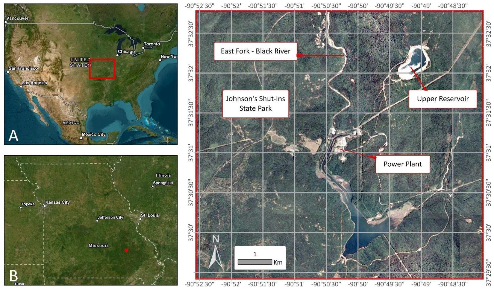
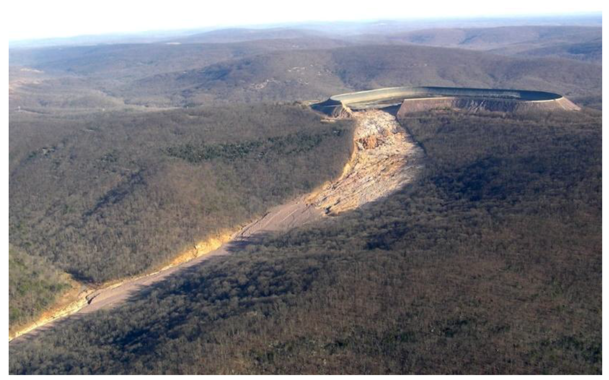
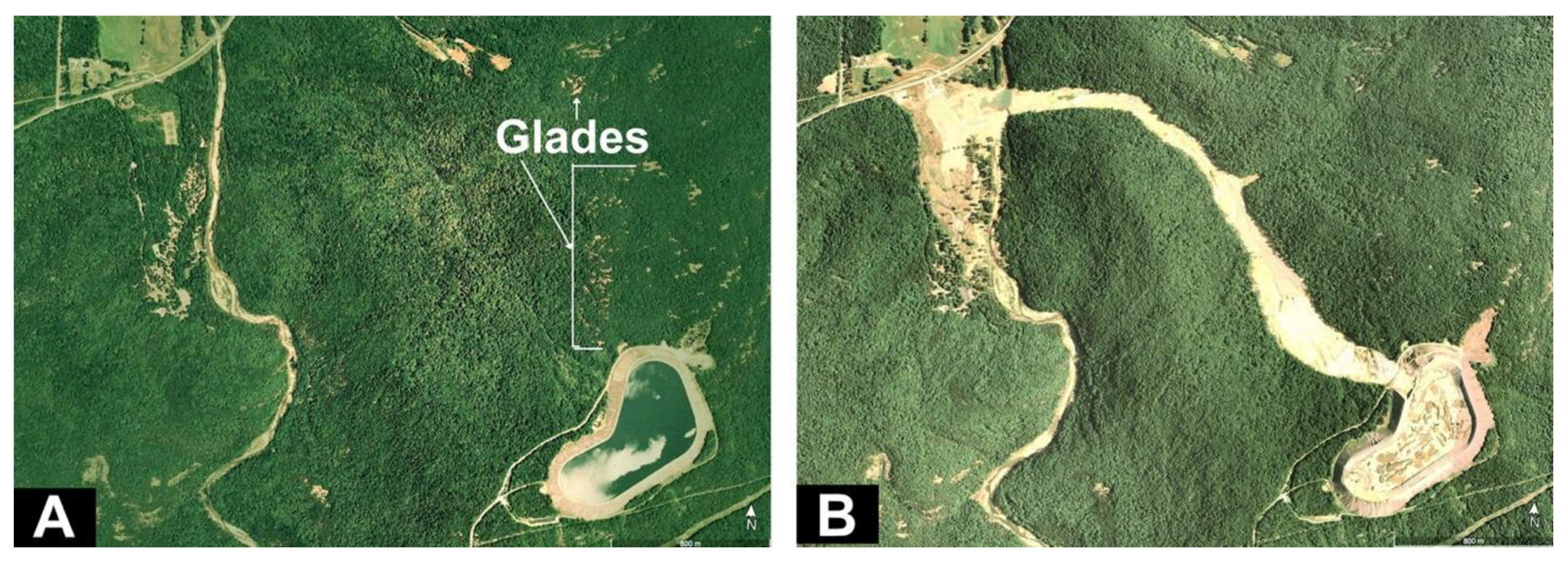
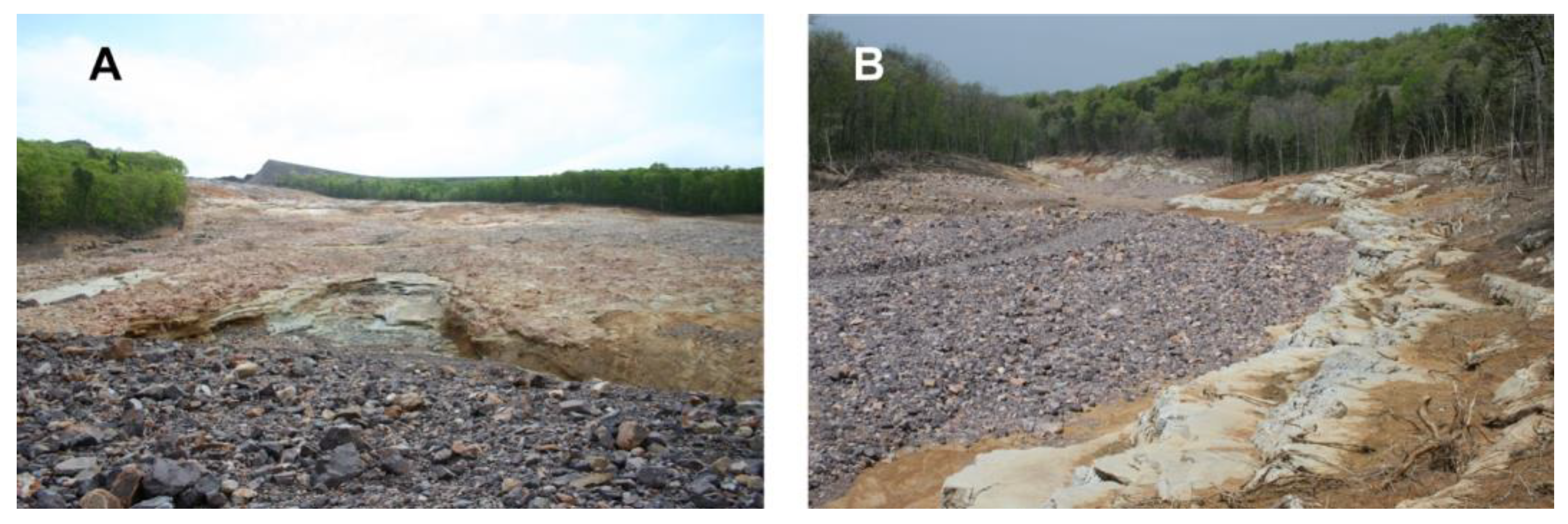
2.1. Study Site

The water from the reservoir breach transported large boulders, sand, clay, uprooted trees, and pieces from the upper reservoir (Figure S1) down the western side of Proffit mountain, and into the campgrounds of Johnson’s Shut-Ins State Park (Figure 3). The water’s path from the upper reservoir to the East Fork of the Black River stripped vegetation and created a scour trail that was 6 m deep, 240 m wide (maximum), and 2.6 km long [2,31]. The lower reservoir absorbed the flood without the lower reservoir dam breaching, but it was left contaminated with natural sediment [2].

The scour site east of the river can be divided into two distinct subsections, upper and lower, based on the underlying geology. Proffit Mountain is part of the St. Francois Mountains, a section of the Ozarks formed from pre-Cambrian volcanic activity between 1.5 and 0.9 BYA [32]. The scour revealed that Proffit Mountain primarily consists of three igneous rock types: rhyolite, rhyolite-derived saprolite (chemically weathered rhyolite), and granite (Figure S2). The igneous section of the scour (upper scour) starts at the top, continues down the steep slope of Proffit Mountain, and abruptly ends at the valley bottom where a geological unconformity (a missing geological record of 700 to 900 million years) occurs [33]; Figure 2 and Figure S3. Because of the steepness of the slope and the hardness of most of the igneous rocks, there was little alluvial deposition on the upper scour (Figure S4).

The remainder of the scour (lower scour), followed a small creek bed in an area geologically defined by sedimentary rocks, primarily conglomerate and dolomite, that were deposited after Cambrian seas inundated the region. Because of the shallower slope, the water lost much of its speed at this point, leading to alluvial deposition up to 6 m deep [33]; Figure 4. When the water came over the igneous rocks and encountered the unconformity, it created a deep plunge pool in the softer sedimentary rocks up to 7.6 m deep [33]; Figures S5 and S6. The alluvial deposits continued for the course of the lower scour, although with less deposition with increasing distance from the breach site. Alluvial deposition continued across the East Fork of the Black River and into Johnson Shut-Ins State Park (Figure S7). Although the central portion of the lower scour was filled with alluvial deposits, the flood did expose dolomite bedrock on the sides of the lower scour (Figure 4).

Restoration work began almost immediately in Johnson’s Shut-Ins State Park, with the park partially reopening in May 2006 and fully reopening in July 2007. Between 2007 and 2009, the upper reservoir of the Taum Sauk Plant was rebuilt, with normal operations resuming in 2010. There was habitat restoration in the upper reservoir area and the state park, with uprooted trees turned to mulch, sand and sediment extracted, and topsoil placed for new grasses and trees.

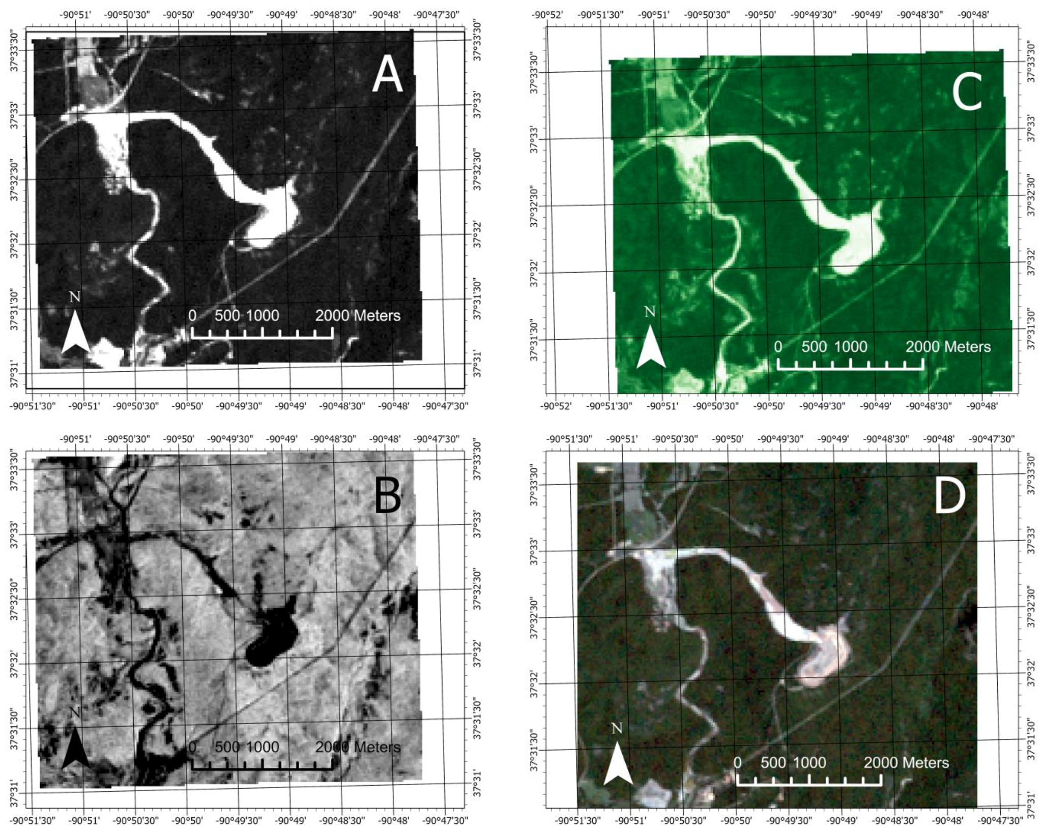
2.2. Satellite Data Collection

The 20 satellite images, with the red (band 3) and NIR (band 4) spectral bands, used to generate the NDVI calculations came from two sources. Landsat imagery, specifically Landsat 5 and Landsat 7, was downloaded from GloVis (Global Visualization Viewer, https://glovis.usgs.gov/, accessed on 15 May 2023) (n = 5), while Rapid-Eye, Dove, and SuperDove imagery were downloaded from Planet Explorer (https://www.planet.com/, accessed on 15 May 2023 for dates through 2020 and 23 January 2025 for dates 2021 to 2024) (n = 15) (

Table 1. Image sources from satellite mission, spatial resolution (m), and dates of images.

Satellite Mission	Spatial Resolution	Dates of Images
Landsat 5	30	16 May 2005 6 July 2006 25 July 2007 25 June 2008
Landsat 7	30	14 May 2013
RapidEye-1	5	14 May 2017
RapidEye-2	5	18 May 2009 30 June 2011 7 July 2018 5 June 2019
RapidEye-3	5	1 May 2015
RapidEye-4	5	8 May 2010 23 June 2012 4 May 2014
RapidEye-5	5	10 June 2016
Dove	3	8 April 2020
SuperDove	3	23 June 2021
SuperDove	3	21 June 2022
SuperDove	3	24 June 2023
SuperDove	3	24 June 2024

). Dates for the images ranged from before the flood (May 2005) to 19 years later (April 2024). Unfortunately, the Landsat images from five years (2005–2008 and 2013) had a lower resolution (30 m) compared to the Rapid-Eye (5 m), Dove (3 m), and SuperDove (3 m) imagery (Table 1). While it would be ideal for all years to have the same spatial resolution, we chose to use higher resolution data (3 m or 5 m) where available to increase the chance of detecting find-scale vegetation recovery over time, which was seen as more appropriate than degrading all data to a lower resolution (30 m). In addition, while 30 m might be considered too low to capture changes in some studies, for this study given the size of the scour (maximum 240 m wide and 2.6 km long), a resolution of 30 m is still capable of generating results that are meaningful, which the ground truthing data supports.

With the GloVis platform, selected images (n = 5) had to entirely encompass the Taum Sauk Plant and scour, as well as align with two criteria: 1) scenes had 0–5% cloud cover, which minimized the amount of vegetation reflectance blocked by clouds, and 2) had acquisition dates between 1 April and 31 July (i.e., when deciduous trees, grasses, and herbaceous plants had leaves), which ensured seasonally vegetation greenness. The downloaded imagery data included TIFF files that store the satellite imagery for each spectral band, with a resolution of 30 m.

With Planet Explorer, SkySat Collect and PlanetScope orthorectified image composite scenes were selected. Only a cloud cover tolerance of 0–5% was permitted, five spectral bands were selected (near-infrared, blue, green, yellow, and red spectral bands), and only surface reflectance was included. The images were downloaded as GeoTIFF files, with Rapid-Eye images (n = 10) at resolution of 5 m, SuperDove images (n = 4) at resolution of 3 m, and the single Dove image at a resolution of 3 m.

All Landsat and Planet imagery used in this analysis was projected into the WGS 1984 UTM Zone 15 N coordinate system. Images were coregistered to a common grid spacing at the highest image resolution (i.e., 3 m pixel spacing) using the GDAL library to facilitate consistent spatial analysis between datasets of differing spatial resolution.

2.3. Remote Sensing and GIS Analysis

2.3.1. Normalized Difference Vegetation Index

NDVI, or Normalized Difference Vegetation Index, is a common metric that quantifies the amount of photosynthetic activity, or greenness, in each pixel of a given satellite image [34]. NDVI contrasts two bands from the multispectral raster dataset (Figure 5), with the red band (R) correlated with chlorophyll pigment absorption and the near-infrared (NIR) band correlated with reflectivity of the plant material [34]. Green leaves have high NIR reflectance and high visible light absorption, compared with water stressed, diseased, or dead leaves, as well as clouds and snow [34]. NDVI was calculated using (1), where values range from –1 to 1 [34]. Healthy and dense vegetation reflects high levels of NIR light but low levels of red visible light (i.e., higher pigment absorption), yielding higher NDVI levels [34]. However, when vegetation is sparse, NIR reflectance decreases and red visible light reflectance increases, yielding lower NDVI levels [34]. NDVI was calculated in a time series from 2005 to 2024 for each multispectral image.

$$NDVI=\left(NIR-R\right)/(NIR+R)$$

(1)

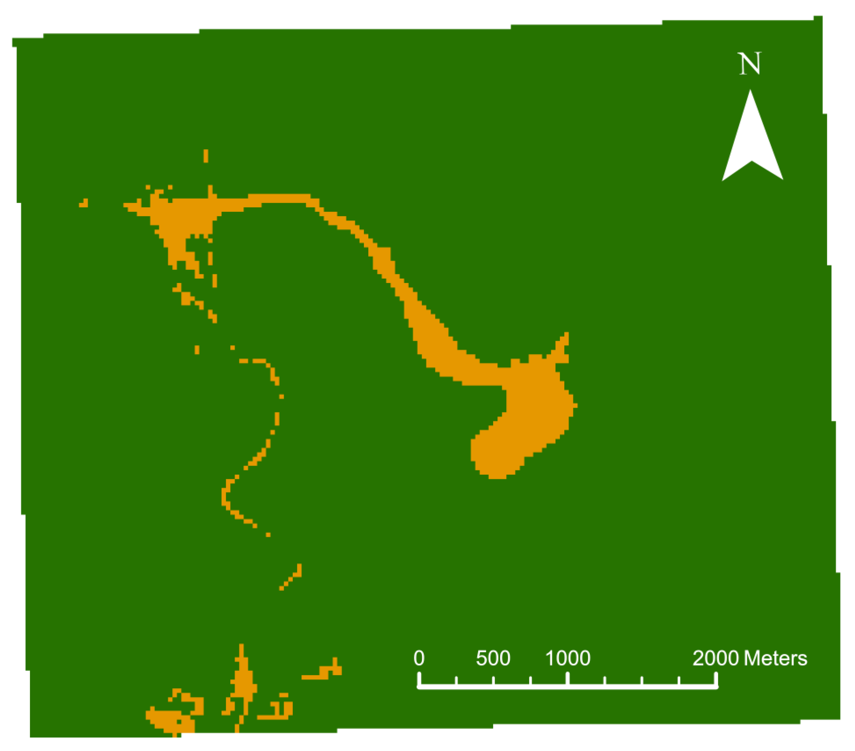
2.3.2. Processing Remotely Sensed Images

Initially, a single image between 8 April and 25 July, when most angiosperms have leaves present, representing the 25.66 km² area around the Taum Sauk Plant, was processed for NDVI levels for each year between 2005 and 2024 (n = 20). The spatial resolution for the calculated NDVI matches the resolution of the original sourced images. Hence, in this analysis, the spatial resolution of NDVI ranges from 3 to 30 m. These individual NDVI images were subsequently reclassified at a pixel-by-pixel basis into two categories: no vegetation or water (NDVI ≤ 0.2) and with vegetation (NDVI > 0.20) [35]. ModelBuilder (ArcMap 10.8) was used to automate calculating NDVI for all 20 downloaded images (Table 1). All outputs were: (1) processed to have identical extents, which aligned with the area of interest, a 25.66 km² area around the Taum Sauk Plant, and (2) reclassified into a binary scale based on NDVI value (Figure 6). Water and no vegetation were grouped and defined by a NDVI ≤ 0.2, with the presence of vegetation indicated by NDVI > 0.2 (Figure 6) [35]. While a small pond was created in the lower scour, its small size would mean only a minor effect on the proportion of area classified as water or no vegetation. Instead, the primary location of water in the scour was the upper reservoir, which was removed from the analyses (see below and Figure 7). The use of a binary division has been used in other analyses evaluating long-term vegetation recovery, including after the industrial flood in Iran where NDVI > 0.3 was equal to strong, dense vegetation and NDVI < 0.3 was equal to weak vegetation [28]. In this study, the cutoff of NDVI = 0.2 was set after testing various binary and multilevel values, with ground truthing used to confirm the cutoff level was sufficient. This cutoff aligns with a comprehensive review of NDVI values related to soil, sparse vegetation or more forested areas, with a cutoff of NDVI = 0.2 showing more accurate results for all three measures in summer images [35].

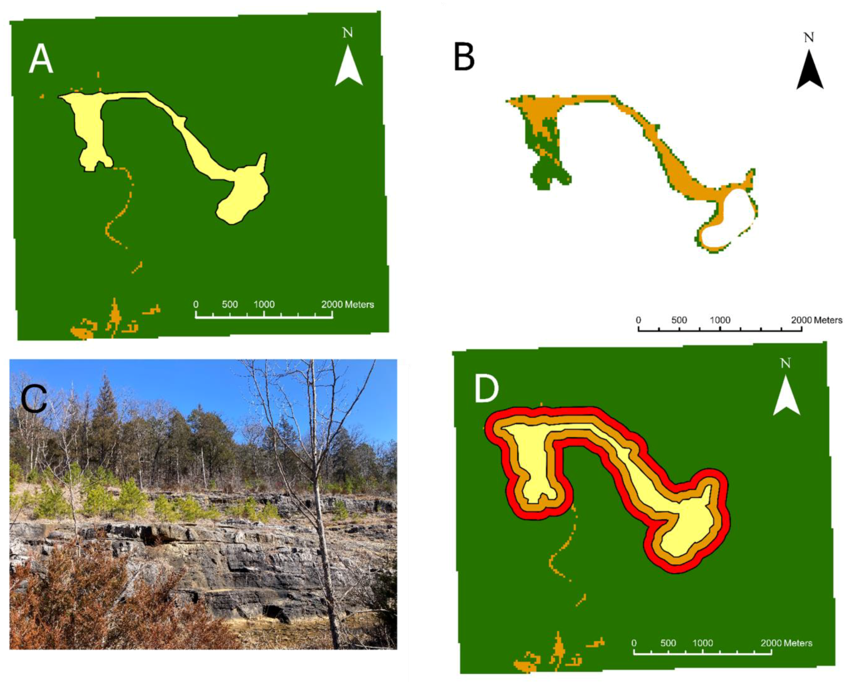
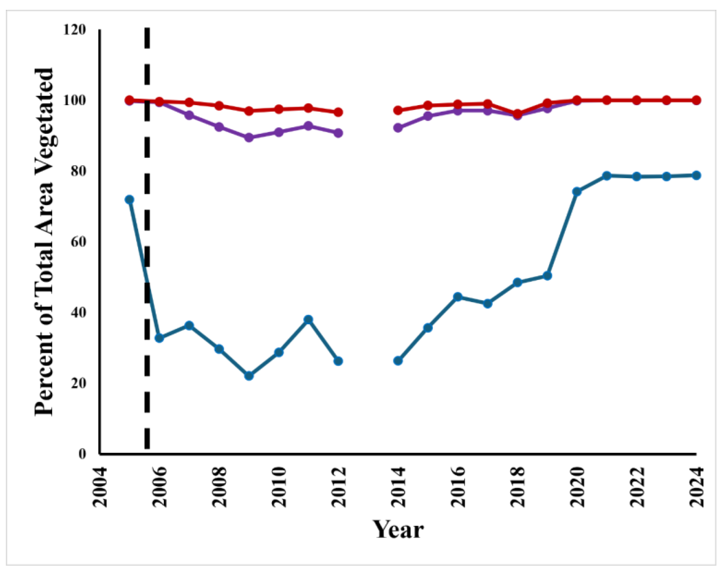
2.3.3. Summarizing NDVI Data

While the initial processing of the satellite imagery showed areas with no vegetation or water (NDVI ≤ 0.2) and areas with vegetation (NDVI > 0.2) in the reservoir (Figure 7B), the latter is believed to be an artifact of water reflectance, as ground truthing prior and after the flood (ART pers. obs.) confirmed the reservoir had no vegetation before the breach and the reservoir was quickly rebuilt after the breach, so detectable vegetation in the reservoir is never possible. To correct for this, the vegetation analyses were narrowed to the scour by using imagery from after the flood (6 July 2006) compared to imagery just prior to the flood (16 May 2005), using the cutoff of NDVI = 0.2 to delineate the sharp contrast between vegetated and non-vegetated areas, which was used as a guide to manually create a polygon that eliminated the reservoir and outlined the scour (Figure 7). For all subsequent analyses, this outline of the scour was used as the maximum extent for evaluating vegetation changes in the time-series analyses.

For all 20 images, the total area within each vegetation type in the scour was calculated based on the proportion of cells, or percentage of total area, that fell into each binary category: no vegetation or with water (NDVI ≤ 0.2) or with vegetation (NDVI > 0.2). While it was not possible to create a confusion matrix, which would determine accuracy of classification (correctly and incorrectly) into the two classes, due to the lack of ground truthing data at the same scale across all years, it was possible to use ground truthing to evaluate accuracy for the pattern of vegetation changes detected by the time-series analyses of remote sensing images. This is further emphasized by the attempt to use other binary and multilevel classifications, which generated inconsistent results that were difficult to interpret, with considerable variation across the images. While there were differences in image resolution, that did not seem to have an impact, as resolution differences were grouped into two time periods: the images from 2005 to 2008 were at the lower resolution of 30 m and those from 2010 to 2024 were at the higher resolution of 3 m or 5 m. The exception to this was the image from 2013 (30 m); however, this image was discarded because of overall poor quality.

To evaluate how the scour compared to the area that extended out from its edge, two 120 m buffers were developed based on the largest width in the scour (240 m), with the proportion of area with and without vegetation within each calculated (Figure 7). Buffer 1 was extended out from the edge of the scour (0–120 m), while Buffer 2 aligned with the outer boundary of Buffer 1 and extended out from this edge (120–240 m).

2.4. Ground Truthing Surveys

Ground truthing surveys were initiated on 19 April 2006, four months after the breach, when safely traversing the scour could be ensured. The survey team consisted of five individuals, although group composition varied (Figure S8). During surveys, team members spread out across the scour, sometimes constrained by physical barriers, walking roundtrip from the top of the scour to the bank of the East Fork of the Black River and back, or the inverse. The narrowness and visual openness of the scour ensured excellent coverage of the scour. Observations of life, including plants, animals, and other life-signs (e.g., tracks, feces), plus the corresponding location, were recorded. The surveys did not include the portion of the scour to the west of the East Fork of the Black River, as it was under habitat restoration by the Missouri Department of Natural Resources and being monitored by the staff naturalist (Janet Price) of Johnson’s Shut-Ins State Park. Nine surveys occurred: 19 April 2006, 1 June 2006, 4 August 2006, 28 July 2009, 20 July 2010, 2 August 2011, 2 May 2012, 14 May 2013, and 19 June 2013. Unfortunately, after 2013, due to multiple reasons, only a single walking survey of the lower scour was possible in 2024, with visual of the upper scour conducted through binoculars, which was possible due to the low levels of tree growth.

The ridge on the eastern side of the upper scour had many Ozark glades (Figure 3A), which are open habitats of exposed bedrock with flora and fauna more typical of deserts and dry prairies, that are embedded within the forests of the Ozarks. The glades above the scour, including ones nearly abutting the reservoir area, were included in ground truthing efforts (2006 and 2009). Because glade flora and fauna are adapted to living in open, rocky environments, it was hypothesized that glades would be a source of colonizing species for much of the scour. It was thought that the eastern collared lizard (Crotaphytus collaris collaris), an apex predator adapted to these areas, could be a bioindicator of vegetation recovery, as it was at the top of the glade community food chain [36]. The protocols for capturing, handling, and sampling of collared lizards were reviewed and approved by The Animal Studies Committee of Washington University (approval number 20100142).

3. Results

3.1. Dynamics of NDVI After the Taum Sauk Dam Failure

For the 25.66 km² area around the Taum Sauk Plant, the minimum (mean = −0.15; range = −0.41 to 0.05) and maximum (mean = 0.84; range = 0.63–0.99) NDVI values were calculated (

Table 2. Summary of 20 satellite images between 2005 and 2024, except for 2013, which was eliminated due to incomplete data. Reported are the minimum and maximum NDVI values for the 25.66 km² area around the Taum Sauk Plant, the % total area no vegetation or with water (NDVI ≤ 0.2) and % total area with vegetation (NDVI > 0.2) for the 1.22 km² area defined to be in the scour, and the 120 m area in each Buffer 1 (0–120 m from the scour) and Buffer 2 (120–240 m from the scour) around the scour.

	Taum Sauk Plant		Scour		Buffer 1		Buffer 2
	NDVI		% NDVI		% NDVI		% NDVI
Year	Minimum	Maximum	≤0.2	>0.2	≤0.2	>0.2	≤0.2	>0.2
2005	−0.08	0.78	28.04	71.96	0.19	99.81	0.00	100.00
2006	−0.26	0.75	67.25	32.75	0.57	99.43	0.37	99.63
2007	−0.08	0.69	63.62	36.38	4.19	95.81	0.61	99.39
2008	−0.11	0.77	70.29	29.71	7.50	92.50	1.52	98.48
2009	−0.16	0.80	77.90	22.10	10.59	89.41	3.04	96.96
2010	−0.18	0.88	71.31	28.69	9.00	91.00	2.55	97.45
2011	−0.18	0.77	61.99	38.01	7.26	92.74	2.23	97.77
2012	−0.31	0.88	73.74	26.26	9.21	90.79	3.41	96.59
2013	---	---	---	---	---	---	---	---
2014	−0.18	0.73	73.67	26.33	7.80	92.20	2.85	97.15
2015	−0.27	0.80	64.31	35.69	4.49	95.51	1.48	98.52
2016	−0.41	0.86	55.59	44.41	2.91	97.09	1.18	98.82
2017	−0.15	0.79	57.43	42.57	2.92	97.08	1.01	98.99
2018	−0.17	0.88	51.49	48.51	4.30	95.70	3.83	96.17
2019	−0.08	0.63	49.61	50.39	2.29	97.71	0.78	99.22
2020	−0.08	0.96	25.78	74.22	0.17	99.83	0.01	99.99
2021	0.03	0.96	21.32	78.68	0.00	100.00	0.00	100.00
2022	0.02	0.97	21.59	78.41	0.04	99.96	0.00	100.00
2023	0.05	0.99	21.52	78.48	0.04	99.96	0.00	100.00
2024	0.01	0.98	21.21	78.79	0.02	99.98	0.00	100.00

) for each year between 2005 and 2024 (n = 20). The highest maximum NDVI value was in 2023 (0.99). Data from 2013 was eliminated from all analyses due to poor data quality.

The first analysis with the binary classification (NDVI ≤ 0.2 and NDVI > 0.2) focused on the 1.22 km² area that corresponded to the scour. After the flood, the percentage of area with vegetation dropped from 71.96% (2005) to 32.75% (2006), with 2009 having the lowest level of vegetation (22.1%; Table 2). This counterintuitive drop in vegetation aligns with the limited habitat restoration in the upper reservoir area, where large vegetative debris (e.g., uprooted trees) was removed from the landscape, as it was turned to mulch. However, in 2020, the proportion of area in the scour with vegetation returned to levels like those prior to the flood (74.22%) and the proportions plateau between 2020 and 2024. There was a sustained low level of areas with no vegetation or water after the flooding event followed by a steady increase in areas with vegetation between 2015 and 2016, at which time a continual and sustained increase was noted (Figure 8).

The other analyses with this binary classification expanded to the two 120 m buffers around the scour to understand patterns of vegetation damage and growth around the scour: Buffer 1 (aligned with scour’s edge at 0–120 m) and Buffer 2 (aligned with Buffer 1’s edge at 120–240 m). While both buffers exhibited similar patterns, where areas with vegetation occupied most of the area, Buffer 1 had slightly lower mean values for the proportion of area with vegetation (mean = 96.13%; range = 89.41–100.00%; Table 2) compared to Buffer 2 (mean = 98.69%; range = 96.17–100.00%; Table 2). Similarly, Buffer 1 had slightly higher mean values for the proportion of area with no vegetation or with water (mean = 3.87%; range = 0–10.59%; Table 2) compared to Buffer 2 (mean 1.31%; range = 0–3.83%; Table 2). Buffer 1 (i.e., the area between the scour and Buffer 2) shows a pattern like that observed in the scour although at a much lower magnitude, with a decline in the proportion of area with vegetation after the flood, followed by an increase in levels starting in 2014 (Figure 8 and Table 2). Buffer 2 shows a more stable pattern in loss and gain, which is representative of the pattern across the broader landscape (Figure 8 and Table 2).

3.2. Ground Truthing Results

3.2.1. Validation of NDVI Inferences

There were repeated on-the-ground surveys of glade communities between 1997 and 2005 on Proffit Mountain and Johnson’s Shut-Ins State Park. as part of the Templeton’s laboratory work on glade communities. Prior to the flood, there were healthy glade communities on the ridge above the scour site, with the dominant community in this area a forest typical for the St. Francois region of the Ozarks, with a canopy of oaks, hickories, and some short-leaf pines. This forested area, which had not been burned in many decades, had a thick woody understory of trees, such as sassafras, redbud, dogwood, wild plum, and service berry. The forest floor was mostly barren of vegetation due to a thick layer of leaf litter and little sunlight [1]. These observations confirm the inferences from the satellite analysis from 2005 that the future scour area was mostly vegetated before the flood (NDVI > 0.2).

Between 2006 and 2013, nine walking surveys over the upper and lower scours were conducted, with one partial survey (primarily lower scour, with remote scans of upper scour) in 2024 (ART pers. obs.).

Table 3. Number of species in various taxa, including invertebrates (Invert), vertebrates (Vert), and small herbaceous plants (small herb), found at the Upper Scour (US), Spring Pond (SPond), Lower Scour (LS), and Lower Scour Pond (LPond) during ground truthing surveys between 2006 and 2012. A summary of the total number of species found in each of the four locations is provided, as well as how many of these species were categorized as species normally found on glades and their associated seeps.

		Taxa
Date	Place	Invert	Vert	Algae	Grasses	SmallHerb	Shrubs	Trees	Total Species	Glade or Seep Species
04/2006	US	3	2	1	1	---	---	---	7	2
	SPond	1	1	1	1	4	---	---	8	4
	LS	---	---	---	---	---	---	---	0	0
	LPond	---	---	---	---	---	---	---	0
Total									15	6
08/2006	US	5	2	1	2	---	---	1	11	5
	SPond	4	2	1	2	2	3	1	15	8
	LS	1	---	---	1	1	1	---	4	2
	LPond	---	---	1	1	---	1	1	4	3
Total									34	18
2009	US	4	4	1	3	5	2	2	21	8
	SPond	3	1	1	3	3	2	2	15	9
	LS	---	---	---	2	1	2	2	7	4
	LPond	---	---	1	2	1	3	2	9	5
Total									52	26
2010	US	---	---	1	3	5	3	2	14	5
	SPond	3	1	1	3	5	2	2	17	9
	LS	---	---	---	2	5	2	2	11	6
	LPond	---	---	1	2	2	3	2	10	5
Total									52	25
2011	US	4	2	1	3	5	4	2	21	10
	SPond	3	2	1	3	6	2	2	19	11
	LS	3	1	---	2	2	2	2	12	9
	LPond	4	1	1	2	3	3	2	16	10
Total									68	40
2012	US	4	2	1	3	5	4	3	22	10
	SPond	4	2	1	4	6	3	2	22	12
	LS	4	2	---	3	4	2	2	17	13
	LPond	5	3	1	4	5	3	2	23	10
Total									84	45

summarizes the results of these surveys, except for the years 2013 and 2024. During the 2013 survey, plant surveys were not possible due to the large number of collared lizards, our bioindicator, captured on the scour, with all time spent handling and processing these animals. The 2024 survey, as previously noted, was only partial and executed by a single person, with the main objective to acquire a qualitative assessment of vegetation in the scour.

While a transect survey design over such a large area is not a reliable method for estimating population sizes, it is possible to report the observed sizes. For the first survey (April of 2006; Table 3), few species were observed, with most of these singleton observations (e.g., Figure S9). Plant exceptions to being a single observation included algae, which was found in an upper scour pool of water fed by a spring that had been exposed by the scour (the Spring Pond; Figures S10 and S11) and several other smaller rock pools. In addition, grasses were found in several sparse clumps around the Spring Pond in areas that had accumulated some soil. The non-singleton animal exception were as follows: (1) two American toads (Bufo americanus; Figure S12) and their tadpoles found in the Spring Pond, as well as in small rock pools in the Upper Scour (Figure S13), and (2) water striders (Aquaris remiges) found in the Spring Pond. Both species were also frequently found to be associated with seeps. Many glades often have acidic seeps within them, where water seeps out from between layers of rhyolite to form a small wetland, thereby providing colonizing species for the wet areas in the scour.

The singleton animal species found on April 2006 were most likely transient individuals, as none of them were adapted to living on bare bedrock habitats but instead are typically woodland species: the Ashborer moth (Podosesia syringae), the scarab beetle (Dichelonyx albicolis), the filmy dome spider (Prolinyphia marginata), and the turkey (Meleagris gallopavo). The Lower Scour alluvial area was devoid of observed life (Figures S14 and S15). In addition, the Lower Scour Pond was highly discolored, due to suspended sediment, and devoid of observable life. Overall, the scour was mostly devoid of observable life, with only small and sporadic clusters of vegetation, consistent with the NDVI results.

These patterns continued for the remainder of the surveys shown in Table 3, with the number of observed species increasing but with many transient singletons, as well as more growth of vegetation around the ponds. There was also growth of grasses and other plants in the rock cracks and ledges of the upper scour where soil was accumulating, and in the lower scour, as soil washed in from the forested edges. Overall, the scour had only sparse vegetation throughout this time, a result that validates the satellite analyses from 2006 to 2012 that consistently inferred low vegetation (NDVI ≤ 0.2) in most of the scour irrespective of the image resolution (30 m or 5 m) and the fact that no major construction projects, or landscape alterations, occurred in this scour area over the seven-year period (2006–2024). While there were no ground truthing surveys in 2007 or 2008, the consistency in low levels of vegetation from 2006 to 2012 in the satellite analyses make it highly improbable that the ground truthing would have found something different in these two years since vegetation was still sparse in 2009. When other binary or multiple-level cutoffs were tried (e.g., NDVI > 0.6) in the satellite analyses, a comparison with the ground truthing data indicated an incompatibility with ground truthing data (e.g., extreme fluctuations in the quantity of highly vegetated areas between 2006 and 2012). The alignment between the satellite analyses, irrespective of data resolution, and ground truthing at a binary division at NDVI = 0.2, provides confidence in the analyses across the broader time scale.

3.2.2. Community Dynamics of the Restoration

While the part of the scour west of the East Fork of the Black River, within Johnson’s Shut-Ins State Park was not included in the ground truthing surveys and is outside of the prevue of this study, ground reports from the staff naturalist of Johnson’s Shut-Ins State Park and visual summaries through satellite photos provide an interesting comparison to the region directly in and around the flood (Figure 3). Prior to the reservoir breach (2005), the area was primarily covered by an oak-hickory forest with a woody understory except for a clearing associated with a campground that accommodated large recreational vehicles (Figure 3A). The summer immediately after the reservoir breach (2006), the scour was mostly barren of vegetation (Figure 3B); however, following active restoration, there was much vegetation only one year later (2007; Figure S16A). By this time, a restoration plan focused on moving the campground to a safer area to the northwest and converting most of the scour area into fields filled with routes for cars and pedestrians. This plan was mostly accomplished by 2010, with the area mostly covered by vegetation (Figure S16B), although not forested as before the flood (Figure 3A). The large-scale active restoration combined with rapid increase in vegetation contrasts with the area directly in and around the upper and lower scour.

Specifically, the situation east of the East Fork of the Black River (i.e., focal area) was more complicated, with almost the entire east scour initially barren and destitute of vegetation (Figure 4, Figures S4 and S14). However, there were three types of areas in which vegetation could be found in April 2006. First, in the upper scour, sparse vegetation, mostly grasses typical of those found on glades, was found on the sides where erosion had brought in some soil from the adjoining forests. Second, the saprolite on the upper scour had experienced significant erosion, producing soil that would accumulate on flat rock shelves and cracks (Figure S17), and areas of pre-Cambrian conglomerate exposed by the scour were also subject to erosion and soil formation (Figure S18). A few grasses and herbaceous plants could be found in these sparsely distributed areas of new soil. Third, vegetation was found near the Spring Pond. The plants (Figure S11) and animals (Figures S12 and S13) observed in the Spring Pond, were the same types of plants that could be found on seeps within glades, with the nearest intact glade being located only 30 m from the upper scour. In only four months after the reservoir breach, the Spring Pond had already attracted a living community of life that is also found in glade seeps.

The portion of the lower scour closest to the upper scour was the most barren portion. Even though much soil had eroded into the lower scour from the sides, there was no detectable live vegetation (Figures S14 and S15). The central part of this portion of the lower scour was characterized by deep deposits of boulders (Figure 4), with no flat areas of solid rock near the surface where soil could quickly accumulate. The only significant vegetation found in the lower scour was the portion close to the East Fork of the Black River, where there was much less deposition of boulders, allowing soils to accumulate on the surface. A large pond was formed in this portion of the lower scour (Figure S16B), which initially had no visible vegetation on its shores; however, only 5.5 months after the reservoir breach, sparse vegetation was evident along its shores (Table 3, Figure S19).

The vegetation, and hence number of plant species, increased over time (Table 3), as more erosion and soil formation occurred from the saprolites on the upper scour and along the sides of the lower scour (Figures S20–S29). As previously mentioned, many of the other animal species observed on the scour were woodland species that could not live permanently on the bare rock or alluvial deposits of the scour. However, some species, not typically found on glades or seeps, were becoming permanently established, including the first two tree species (willows and poplars) found near the ponds (Table 3). Nevertheless, overall, 40% of the species observed on the scour during the April 2006 survey were associated with glades and their seeps (Table 3), a large enrichment given that glades represent only a tiny portion of the overall landscape and species existing on this landscape. Over time, the number of permanent species found on the scour increased, mostly derived from the glade and seep communities. For example, by August of 2006, the Spring Pond acquired whirligig beetles (Gyrinus substriatus) and the woodland crayfish (Faxonius hylas), both also found on seeps. In addition, the grassy areas of the scour had also acquired the grasshopper (Hippiscus ocelote), a glade species. This increase in glade and seep species continued throughout these surveys, including in 2009 when there were five orthopteran species, typically limited to glades, found on the scour. A thorough survey of orthopteran species on nearby Taum Sauk Mountain found 20 different orthopteran species on glades that were not present in the surrounding unburned woodlands [36]. The fact that the single-day transect surveys, over such a large area, found only a quarter of these glade orthopteran species was not unexpected because such transect surveys typically miss or undercount many species. Even with this caveat, the enrichment of glade and seep associated species is seen with the percent species at 40% in April 2006 increasing to 59% in 2011 and 54% in 2012, with the latter having less time for survey of other taxa due to the larger number of collared lizards, another glade species captured, processed, and released (Table 3).

Although there were increasing amounts of vegetation after 2009, the original vegetation of a forest dominated by oaks and hickory trees, with a thick woody understory, still has not recovered even by 2024 (Figure S30). Instead, the alluvial lower scour was now covered with grasses, shrubs, and a few trees (Figure S30), and the same was true for the upper scour, but the vegetation was sparser compared to the lower scour (Figure S30). Several trees were now growing all over the upper scour, and not just at Spring Pond. Most of these new trees were oaks and short-leaf pine, but the upper scour still had no closed canopy as before the flood (Figures S30 and S31). Many of these trees were still small in 2024, particularly the short-leaf pines, so the vegetation height of most of the scour throughout the entire recovery was low because it was dominated by grasses, small herbaceous plants, shrubs, and tree saplings. The taller trees were concentrated in the areas formally dominated by beds of saprolite, which had now been eroded into soil (Figure S31). Soil deposition had also occurred in the lower scour, filling in many of the cracks and crevices among the alluvial deposits and allowing much growth of grasses and shrubs (Figure S30).

3.2.3. Collared Lizards as a Bioindicator

No eastern collared lizards were observed on the scour in 2006, However, their scat, which is distinctive from other lizard scat, was observed in the upper scour in 2009, indicating transient exploration of the scour by eastern collared lizards, probably from nearby glades (Figure 9). No lizards or scat were observed in 2010, but the survey occurred after a hard rain the night before that would have washed scat away. In 2011, eastern collared lizard scat was observed in the upper scour but no lizards (Figure 9). In 2012 and 2013, many eastern collared lizards were observed, but mostly in the lower scour (Figure 9).

4. Discussion and Conclusions

4.1. The Dynamic Change Pattern of Vegetation After Disturbance

The time series analysis of the NDVI values of the area in and around the flood scour at the Taum Sauk Plant, from just prior to the flood (2005) through to 2024, allowed for the natural plant growth and vegetation succession to be observed following the reservoir breach. While efforts were made to clear natural and other debris after the reservoir failure [37], most of the plant growth and succession in and around the scour are due to natural causes. Focused on the scour (Figure 8 and Table 2), the NDVI pattern reveals a dramatic loss of vegetation following the flood, with vegetation levels varying for several years, before a steady increase in the proportion of areas with vegetation started in 2014. The buffer adjacent to the scour (Buffer 1) showed a similar, although less dramatic, pattern (Figure 8 and Table 2), which likely reflects the ragged edge created by the flood, with vegetation and ground shifting not just in the scour but for some distance along its edge. This contrasts with the buffer representative of the broader landscape (Buffer 2) that showed no sustained patterns of increase or decrease (Figure 8 and Table 2). In summary, the behavior of Buffer 1 is intermediary to that found in the scour and Buffer 2.

The reason for the overall sparseness of vegetation in and around the scour between 2006 and 2013 was most likely the lack of soil to support plant growth. Although the saprolite and conglomerate beds showed some erosion in less than a year after the flood (2006, Figures S6, S17, S19 and S20), and much additional erosion though 2013, most of this new soil could accumulate only in cracks and crevices in the bedrock of the upper scour, with any soil washed into the lower scour filling crevices in the alluvial rocky deposits of the lower scour, locations far from sunlight due to the depth of these deposits. The continuous increase in vegetation in the scour from 2014 to 2020 (Figure 8) was most likely explained by the filling of soil into the crevices in the lower scour and for soil regions expanding from the initial cracks into the upper scour, due to the initial plant growth that would broaden the area of soil accumulation. This explanation is consistent with what was witnessed in 2024, with the saprolite beds completely eroded and covered with vegetation, even trees (Figure S31), and the alluvial deposits in the lower scour filled with soil upon which grasses and shrubs grew (Figure S30). Hence, soil formation, and perhaps soil erosion into the scour from the forested sides of the scour (Figure S23), were critical for biological recovery.

Ground truthing surveys performed between 2006 and 2013 confirmed that much of the scour was barren but the amount and type of vegetation was slowly increasing (Table 3). However, this increase in vegetation was not spatially uniform across the scour, but rather concentrated at the sides of the scour (Figures S23, S24 and S27), in those areas associated with soil accumulation (Figures S21, S25 and S29), and along ponds and creeks (Figures S22 and S26). The most dense and diverse vegetation first appeared in the lower scour near where the scour crossed the East Fork of the Black River (Figure S28), but these vegetated areas represent only a small portion of the scour. However, even though NDVI with remote sensing indicated that the vegetation was still sparse in 2012, the ground truthing surveys revealed that two isolated and small areas in the scour had gained sufficient vegetation to support a population of arthropods, such as grasshoppers (i.e., the primary food for eastern collared lizards), which allowed for the reproduction and growth of the eastern collared lizard (a vertebrate predator) within the scour (Figure 9).

4.2. Bioindicators for Vegetation Recovery After the Taum Sauk Dam Failure

Many of the plants and animals found in the scour were found on the rhyolitic glades and seeps on the ridge above the scour (Table 3), and the proportion of species found on the scour that were species from glades and their seeps tended to increase with time (Table 3). This pattern indicates that the glades and seeps on the ridges above the scour were essential for the initial biological recovery of the scour. While glades and acidic seeps, seen as tiny light-colored dots in the extensive green forested areas (Figure 3A and Figure 9), represented only a tiny fraction of the pre-flooded landscape, they played a dominant role in the restoration of life into the scour (Table 3), an observation that supports the hypothesis that landscapes with high levels of habitat and species diversity are more resilient to perturbations than less diverse landscapes [38,39]. Therefore, in this case, habitat restoration was less about species diversity per se and rather about habitat diversity within a landscape, with even rare habitats playing a disproportionate role in restoration (Table 3).

Direct confirmation of these glades and their associated seeps serving as a source for species colonizing the scour is possible through observations on the eastern collared lizard (Figure S32), which is the only lizard found exclusively on glades in this area of the Ozarks. The eastern collared lizard is an apex predator in the glade communities, which means they are a sensitive biomarker for the health of the broader glade community, including its flora [36]. Only scat was observed between 2009 and 2011, all in the upper scour. Even though all surveys were conducted on warm, sunny days with the exception of 2010, no lizards were observed perching on high rocks to visually scan for prey and to signal territorial ownership [40], which indicates that as of 2011, no territories had been established in the scour. Nevertheless, the presence of scat supports their exploration of the area. The lack of territories in the upper scour indicates it lacked sufficient vegetation to support this apex predator, as the scour was well within the dispersal distances (as little as 30 m between the glade and scour) possible by individual lizards > 2 km [41].

By 2012–2013, 35 eastern collared lizards were observed in the upper and lower scours (Figure 9). Of these lizards, three were hatchlings, six were yearlings, and seven were captured in the same general area in both years, indicating that the lizards had established territories and were reproducing in the scour. However, most of the lizards, including most of the females and hatchlings, were found near the lower scour pool, which was the area that ground truthing had shown to have the greatest amount of vegetation in the entire scour (Figure S28). Another area that had both males and females was found upstream but still in the lower scour at a site where a creek entered the main valley (Figure 9). This creek provided additional water that made this local area more vegetated than most of the lower scour except for the lower scour pool area. Hence, male and female eastern collared lizards were only found in the most vegetated areas of the scour, and these areas had developed a fully functional, three-trophic level glade community by 2012.

The remaining captures of eastern collared lizards were at the intersection of the upper and lower scours (Figure 9), where the plunge pools at this intersection collected much soil (Figure S6) and produced a narrow band of vegetation; however, only males were found at this intersection. Male collared lizards are extremely aggressive about defending their territories, with the males unable to defend a territory frequently found in marginal areas that have insufficient vegetation to support female reproductive territories. This area inhabited exclusively by males indicates that it was marginal in vegetation, which was supported by ground truthing. The lack of females and hatchlings in this area indicates that the sparse vegetation found at the intersection of the upper and lower scours was insufficient to support a functional glade community by 2013.

By 2024, the original oak/hickory forest community that dominated the area prior to the flood has yet to be restored to the scour, suggesting that resilience is not necessarily the same as stability. Nevertheless, many species from forest communities (e.g., oaks and pines; Figure S31) had now became established in the scour. As a result, the scour, by 2024, was teeming with life that represented a mixture of species that came from diverse surrounding habitats such as glades, seeps and woodlands. This role of habitat diversity contributing to resilience, in addition to species diversity, is an important conclusion given the rapid environmental changes and challenges that the world is currently experiencing.

4.3. The Limitations and Outlook

There were a few limitations associated with the satellite image analyses. First, the 2013 image had regions lacking data due to a Landsat 7 Scan Line Corrector Failure, which caused the image to have data gaps. With no other images available based on the selection criteria, this year was eliminated from all analyses. Second, the variation in acquisition parameters found across the 20 images, which were collected from various satellites, resulted in imagery having variable sensitivity to cloud cover, which resulted in spatiotemporal variation in the NDVI between and among years. While this would be an issue when using the full scale of individual NDVI values, the use of a binary classification of NDVI = 0.2, a value based on published studies [28,35], eliminates issues related to this variation between images.

Although full ground truthing surveys were only possible until 2013, these data provided interesting insights and support to the NDVI analyses, with remote sensing data that provided insights into the recovery of a landscape after an outburst flood. The NDVI analyses indicated a sharp drop in vegetation in the area in and around the scour after the catastrophic failure (2005), with little indication of widespread recovery until after 2012–2013, with 2013 not having NDVI data available (Figure 8). These patterns matched the ground truthing surveys, with vegetation in almost all of the area in and around the scour being extremely sparse, except for three small areas: the Spring Pond in the upper scour, the side-creek entrance in the lower scour, and the pond in the lower scour. While the biological success and restoration within the scour was invisible even to high-resolution remote sensing (5 m; Figure 8), ground truthing indicated that by 2012, a functioning community of at least three trophic levels had been established within the scour (Figure 9). After 2014 and going forward to 2024, both remote sensing and ground truthing surveys aligned, with an increase in vegetation that eventually covered most of the scour. These patterns, similarities and differences highlight the benefits of using an approach that uses multiple techniques that play complementary roles in monitoring vegetation and landscape recovery after an outburst flood. In this case, the use of time-series analyses with the NDVI, plus ground truthing, allowed for knowledge on recovery to extend beyond vegetation and allowed us to see how the presence of bioindicators (i.e., eastern collared lizard) can indicate ongoing fine-scale changes for vegetation that have a delayed appearance in even high-resolution remote sensing images.

5. Future Directions

Future studies focused on the Taum Sauk Plant could expand to include additional seasons, the types of vegetation and plants that are growing in the scour, and how specific plants have been impacted by the flood, with some species being more resilient than others. While this investigation is focused on one manmade disaster in a single region, the methods and approach can have a broader application to understand how vegetation is affected and how it recovers after natural disasters (e.g., volcanic eruptions, landslides, tornados), with the frequency of such events increasing annually [42].

References

1. Rogers, J.D.; Watkins, C.M.; Chung, J.W. The 2005 upper Taum Sauk dam failure: A case history. Environ. Eng. Geosci. 2010, 16, 257–289. [Google Scholar] [CrossRef]
2. Watkins, C.M.; Rogers, J.D. Overview of the Taum Sauk Pumped Storage Power Plant Upper Reservoir Failure, Reynolds County, MO. In Proceedings of the International Conference on Case Histories in Geotechnical Engineering, Arlington, VA, USA, 11–16 August 2008; Missouri University of Science and Technology: Rolla, MO, USA, 2008; pp. 1859–1879. [Google Scholar]
3. Mei, S.; Zhong, Q.; Yang, M.; Chen, S.; Shan, Y.; Zhang, L. Overtopping-Induced breaching process of concrete-faced rockfill dam: A case study of Upper Taum Sauk dam. Eng. Fail. Anal. 2023, 144, 106982. [Google Scholar] [CrossRef]
4. Askar, S.; Peyma, S.Z.; Yousef, M.M.; Prodanova, N.A.; Muda, I.; Elsahabi, M.; Hatamiafkoueieh, J. Flood Susceptibility Mapping Using Remote Sensing and Integration of Decision Table Classifier and Metaheuristic Algorithms. Water 2022, 14, 3062. [Google Scholar] [CrossRef]
5. Atefi, M.R.; Miura, H. Detection of Flash Flood Inundated Areas Using Relative Difference in NDVI from Sentinel-2 Images: A Case Study of the August 2020 Event in Charikar, Afghanistan. Remote Sens. 2022, 14, 3647. [Google Scholar] [CrossRef]
6. Garajeh, M.K.; Weng, Q.H.; Haghi, V.H.; Li, Z.; Garajeh, A.K.; Salmani, B. Learning-Based Methods for Detection and Monitoring of Shallow Flood-Affected Areas: Impact of Shallow-Flood Spreading on Vegetation Density. Can. J. Remote Sens. 2022, 48, 481–503. [Google Scholar] [CrossRef]
7. Nab, A.W.; Kumar, V.; Rajapakse, R. Innovative methods for rapid flood inundation mapping in Pul-e-Alam and Khoshi districts of Afghanistan using Landsat 9 images: Spectral indices vs. machine learning models. Model. Earth Syst. Environ. 2024, 10, 2495–2513. [Google Scholar] [CrossRef]
8. Abrar, M.F.; Iman, Y.E.; Mustak, M.B.; Pal, S.K. Assessment of vulnerability to flood risk in the Padma River Basin using hydro-morphometric modeling and flood susceptibility mapping. Environ. Monit. Assess. 2024, 196, 661. [Google Scholar] [CrossRef]
9. Al-Kindi, K.M.; Alabri, Z. Investigating the Role of the Key Conditioning Factors in Flood Susceptibility Mapping Through Machine Learning Approaches. Earth Syst. Environ. 2024, 8, 63–81. [Google Scholar] [CrossRef]
10. Arabameri, A.; Saha, S.; Chen, W.; Roy, J.; Pradhan, B.; Bui, D.T. Flash flood susceptibility modelling using functional tree and hybrid ensemble techniques. J. Hydrol. 2020, 587, 125007. [Google Scholar] [CrossRef]
11. Bui, D.T.; Khosravi, K.; Shahabi, H.; Daggupati, P.; Adamowski, J.F.; Melesse, A.M.; Pham, B.T.; Pourghasemi, H.R.; Mahmoudi, M.; Bahrami, S.; et al. Flood Spatial Modeling in Northern Iran Using Remote Sensing and GIS: A Comparison between Evidential Belief Functions and Its Ensemble with a Multivariate Logistic Regression Model. Remote Sens. 2019, 11, 1589. [Google Scholar] [CrossRef]
12. Chithra, K.; Binoy, B.V.; Bimal, P. Modeling flood susceptibility on the onset of the Kerala floods of 2018. Environ. Earth Sci. 2019, 83, 123. [Google Scholar] [CrossRef]
13. Hoang, D.V.; Liou, Y.A. Assessing the influence of human activities on flash flood susceptibility in mountainous regions of Vietnam. Ecol. Indic. 2024, 158, 111417. [Google Scholar] [CrossRef]
14. Yang, H.L.; Yao, R.; Dong, L.Y.; Sun, P.; Zhang, Q.; Wei, Y.; Sun, S.; Aghakouchak, A. Advancing flood susceptibility modeling using stacking ensemble machine learning: A multi-model approach. J. Geogr. Sci. 2024, 34, 1513–1536. [Google Scholar] [CrossRef]
15. Ghosh, A.; Chatterjee, U.; Pal, S.C.; Towfiqul Islam, A.R.M.; Alam, E.; Islam, M.K. Flood hazard mapping using GIS-based statistical model in vulnerable riparian regions of sub-tropical environment. Geocarto Int. 2023, 38, 2285355. [Google Scholar] [CrossRef]
16. Kumar, R.; Acharya, P. Flood hazard and risk assessment of 2014 floods in Kashmir Valley: A space-based multisensor approach. Nat. Hazards 2016, 84, 437–464. [Google Scholar] [CrossRef]
17. Rihan, M.; Mallick, J.; Ansari, I.; Islam, M.R.; Hang, H.T.; Shahfahad; Rahman, A. Flash flood susceptibility modeling using optimized deep learning method in the Uttarakhand Himalayas. Earth Sci. Inform. 2025, 18, 24. [Google Scholar] [CrossRef]
18. Singha, C.; Swain, K.C.; Meliho, M.; Abdo, H.G.; Almohamad, H.; Al-Mutiry, M. Spatial Analysis of Flood Hazard Zoning Map Using Novel Hybrid Machine Learning Technique in Assam, India. Remote Sens. 2022, 14, 6229. [Google Scholar] [CrossRef]
19. Stateczny, A.; Praveena, H.D.; Krishnappa, R.H.; Chythanya, K.R.; Babysarojam, B.B. Optimized Deep Learning Model for Flood Detection Using Satellite Images. Remote Sens. 2023, 15, 5037. [Google Scholar] [CrossRef]
20. Nhu, V.H.; Ngo, P.T.T.; Pham, T.D.; Dou, J.; Song, X.; Hoang, N.D.; Tran, D.A.; Cao, D.P.; Aydilek, I.B.; Amiri, M.; et al. A New Hybrid Firefly-PSO Optimized Random Subspace Tree Intelligence for Torrential Rainfall-Induced Flash Flood Susceptible Mapping. Remote Sens. 2020, 12, 2688. [Google Scholar] [CrossRef]
21. Qin, X.L.; Shi, Q.; Wang, D.Z.; Su, X. Inundation Impact on Croplands of 2020 Flood Event in Three Provinces of China. IEEE J. Sel. Top. Appl. Earth Obs. Remote Sens. 2022, 15, 3179–3189. [Google Scholar] [CrossRef]
22. Shrestha, R.; Di, L.P.; Yu, E.G.; Kang, L.; Shao, Y.Z.; Bai, Y.Q. Regression model to estimate flood impact on corn yield using MODIS NDVI and USDA cropland data layer. J. Integr. Agric. 2017, 16, 398–407. [Google Scholar] [CrossRef]
23. Wang, Q.; Watanabe, M.; Hayashi, S.; Murakami, S. Using NOAA AVHRR data to assess flood damage in China. Environ. Monit. Assess. 2003, 82, 119–148. [Google Scholar] [CrossRef] [PubMed]
24. Isaacson, S.; Armoza-Zvuloni, R.; Babad, A.; Swiderski, N.B.; Segev, N.; Shem-Tov, R.; Stavi, I. Mass tree uprooting during a mega flash flood in the hyper-arid Wadi Zihor, southern Israel. Catena 2024, 242, 108133. [Google Scholar] [CrossRef]
25. Silveira, E.M.D.O.; Acerbi, F.W.; de Mello, J.M.; Bueno, I.T. Object-based change detection using semivariogram indices derived from NDVI images: The environmental disaster in Mariana, Brazil. Cienc. E Agrotecnol. 2017, 41, 554–564. [Google Scholar] [CrossRef]
26. Verma, S.; Sharma, A.; Yadava, P.K.; Gupta, P.; Singh, J.; Payra, S. Rapid flash flood calamity in Chamoli, Uttarakhand region during Feb 2021: An analysis based on satellite data. Nat. Hazards 2022, 112, 1379–1393. [Google Scholar] [CrossRef]
27. Yang, Z.; Wei, J.; Deng, J.; Gao, Y.; Zhao, S.; He, Z. Mapping Outburst Floods Using a Collaborative Learning Method Based on Temporally Dense Optical and SAR Data: A Case Study with the Baige Landslide Dam on the Jinsha River, Tibet. Remote Sens. 2021, 13, 2205. [Google Scholar] [CrossRef]
28. Taherizadeh, M.; Khushemehr, J.H.; Niknam, A.; Nguyen-Huy, T.; Mezősi, G. Revealing the effect of an industrial flash flood on vegetation area: A case study of Khusheh Mehr in Maragheh-Bonab Plain, Iran. Remote Sens. Appl. Soc. Environ. 2023, 32, 101016. [Google Scholar] [CrossRef]
29. Lu, T.; Zeng, H.; Luo, Y.; Wang, Q.; Shi, F.; Sun, G.; Wu, Y.; Wu, N. Monitoring vegetation recovery after China’s May 2008 Wenchuan earthquake using Landsat TM time-series data: A case study in Mao County. Ecol. Res. 2012, 27, 955–966. [Google Scholar] [CrossRef]
30. Peña, M.A.; Ulloa, J. Mapping the post-fire vegetation recovery by NDVI time series. In Proceedings of the First IEEE International Symposium of Geoscience and Remote Sensing, Valdivia, Chile, 15–16 July 2017; IEEE: Piscataway, NJ, USA, 2017; pp. 1–8. [Google Scholar]
31. Luna, R.; Wronkiewicz, D.J.; Rydlund, P.; Krizanich, G.W.; Shaver, D.K. Evaluation of the Taum Sauk Upper Reservoir Failure Using LiDAR. In Proceedings of the GeoDenver 2007 Conference, Denver, CO, USA, 18–21 February 2007; American Society of Civil Engineers: Denver, CO, USA, 2007. [Google Scholar]
32. Unklesbay, A.G.; Vinyard, J.D. Missouri Geology; University of Missouri Press: Columbia, MO, USA, 1992. [Google Scholar]
33. Brinkley, D.; George, S. Geology and Hydrology Inspection—Profitt Mountain Channel; MACTEC, Inc., MACTEC Engineering and Consulting: Alpharetta, GA, USA, 2006. [Google Scholar]
34. Pettorelli, N. The Normalized Difference Vegetation Index; Oxford University Press: New York, NY, USA, 2013. [Google Scholar]
35. Montandon, L.; Small, E. The impact of soil reflectance on the quantification of the green vegetation fraction from NDVI. Remote Sens. Environ. 2008, 112, 1835–1845. [Google Scholar] [CrossRef]
36. Templeton, A.R.; Neuwald, J.L.; Conley, A.K. Life history changes in the eastern collared lizard in response to varying demographic phases and management policies. Popul. Ecol. 2024, 66, 53–67. [Google Scholar] [CrossRef]
37. Toledo, M.Á.; Morán, R.; Oñate, E. Dam Protections Against Overtopping and Accidental Leakage; CRC Press: Boca Raton, FL, USA, 2015. [Google Scholar]
38. Capdevila, P.; Stott, I.; Oliveras Menor, I.; Stouffer, D.B.; Raimundo, R.L.G.; White, H.; Barbour, M.; Salguero-Gómez, R. Reconciling resilience across ecological systems, species and subdisciplines. J. Ecol. 2021, 109, 3102–3113. [Google Scholar] [CrossRef]
39. Holling, C.S. Resilience and Stability of Ecological Systems. Annu. Rev. Ecol. Evol. Syst. 1973, 4, 1–23. [Google Scholar] [CrossRef]
40. Conley, A.K.; Neuwald, J.L.; Templeton, A.R. Network analyses of the impact of visual habitat structure on behavior, demography, genetic diversity, and gene flow in a metapopulation of collared lizards (Crotophytus collaris collaris). In New Horizons in Evolution; Wasser, S.P., Frenkel-Morgenstern, M., Eds.; Oxford Academic Press: Oxford, UK, 2021; pp. 131–160. [Google Scholar]
41. Templeton, A.R.; Brazeal, H.; Neuwald, J.L. The transition from isolated patches to a metapopulation in the eastern collared lizard in response to prescribed fires. Ecology 2011, 92, 1736–1747. [Google Scholar] [CrossRef] [PubMed]
42. Sabins, F.F., Jr.; Ellis, J.M. Remote Sensing: Principles, Interpretation, and Applications; Waveland Press: Lake Zurich, IL, USA, 2020. [Google Scholar]
Figure 1. Relative location of the Taum Sauk Plant in the United States shown by the red rectangle enclosing the state of Missouri (A) and within Missouri shown by the red dot (B), with the area around the Taum Sauk Plant before the flood shown in detail [Source: Google Earth image from 18 August 2005].
Remotesensing 17 01605 g001
Figure 2. Aerial photo of the Taum Sauk upper reservoir and scour the day after the reservoir breach (15 December 2005). The location where a small, seasonal creek enters the scour can be seen in the lower-left corner. Credit: AR Templeton.
Remotesensing 17 01605 g002
Figure 3. Google Earth satellite photos of the study site: (A) August 2005, or prior to the reservoir failure, with the location of glades (open, rocky habitats on exposed bedrock) shown on the ridge immediately above the scour, and (B) July 2006, or seven months after the breach, with the location where a small seasonal creek enters the scour seen as the notch coming off the lower scour.
Remotesensing 17 01605 g003
Figure 4. Photos from four months after the reservoir breach (19 April 2006). (A) Bottom of the igneous upper scour and the beginning of the sedimentary lower scour, with much alluvial deposition. (B) Exposed dolomite on sides of the lower scour. Credit: AR Templeton.
Remotesensing 17 01605 g004
Figure 5. Example (6 July 2006) of spectral band images used to calculate NDVI: (A) red and (B) near-infrared (NIR). Panel (C) shows the NDVI values calculated from these two spectral bands, with green corresponding to high NDVI and white corresponding to low NDVI. Panel (D) shows the true color image.
Remotesensing 17 01605 g005
Figure 6. Example of reclassified binary NDVI output that represents areas with no vegetation or water (orange; NDVI ≤ 0.2) and areas with vegetation (green; NDVI > 0.2). See Supplementary File for outputs from all 20 years (2005–2024).
Remotesensing 17 01605 g006
Figure 7. (A) Polygon (yellow) defining the scour generated by the flood that was used in the refined analyses that removes the reservoir (far right). (B) Example (6 July 2006) of the NDVI file following this extraction that focuses on only the scour, showing areas with (green) and without vegetation (orange). (C) View of the edge of the scour on 2 March 2024, where the two 120 m buffers were added, showing the exposed rock and forest edge caused by the flood. Credit: AA Peterson. (D) A polygon of the scour (yellow), with the two buffers along its edge: Buffer 1 at 0–120 m (orange) and Buffer 2 (120–240 m) (red).
Remotesensing 17 01605 g007
Figure 8. Scatter plots for proportion (%) total area vegetated (NDVI > 0.2) within the scour (blue), Buffer 1 (0–120 m from scour; purple), and Buffer 2 (120–240 m from scour; red) for the 19 summer images between 2005 and 2024. The data for 2013 was eliminated from analysis and scatter plots due to missing data (i.e., poor image quality). The time of the catastrophic failure (14 December 2005) is indicated by the dashed line.
Remotesensing 17 01605 g008
Figure 9. Results of eastern collared lizard (Crotaphytus collaris collaris) surveys, which includes scat found in 2009 (black) and 2011 (dark brown), as well as live lizards found in 2012 (red) and 2013 (green). The sex of the live lizards, male (M) or female (F), is indicated next to the corresponding points in both years. An H by the location point indicates a hatchling lizard whose sex could not be determined. A white oval near the reservoir end of the scour encircles the glade closest to the scour that had collared lizards on it.
Remotesensing 17 01605 g009