Development of a Distance-Adaptive Gaussian Fitting Method for Scheimpflug LiDAR-Based Plant Phenotyping

Abstract

Lidar has emerged as a pivotal technique within the booming field of plant phenotyping, which has seen significant advancements in recent years. Beyond the conventional LiDAR systems that determine distance based on time-of-flight principles, Scheimpflug LiDAR, an emerging technique proposed within the past decade, has also expanded its field to plant phenotyping. However, early applications of Scheimpflug LiDAR were predominantly focused on aerosol detection, where stringent requirements for range resolution were not paramount. In this paper, a detailed description of a Scheimpflug LiDAR designed for plant phenotyping is proposed. Furthermore, to ensure high-precision scanning of plant targets, a distance-adaptive Gaussian fitting methodology is proposed to improve the spatial precision from 0.1781 m to 0.044 m at 10 m, compared with the traditional maximum method. The results indicate that the point cloud data acquired through our method yield more precise phenotyping outcomes, such as diameter at breast height (DBH) and plant height. This paves the way for further application of the Scheimpflug LiDAR on growth stages monitoring and precision agriculture.

1. Introduction

To meet the world’s ever-growing population and limited cultivated area, a deep understanding of plants, especially how the environment and gene affect their growth, is required [1]. Thus, the field of plant phenotyping, which focuses on the research of physical, physiological, and biochemical characteristics of plant structure and growth status, is booming [2]. Traditional plant phenotypic analysis relies on manual measurements, which cost a lot of labor, and the data collected are often not fine enough. In recent years, RGB or monochromatic cameras [3,4], hyperspectral cameras [5], LiDAR [6], and other sensor technologies have been involved in the high-throughput analysis of plant phenotypic characteristics [7] and show great potential.

As a high-precision detection technology, LiDAR owns the advantages of a long detection range, high precision, high data collection efficiency, etc. It has been widely applied to the monitoring of the atmosphere, water bodies, environmental pollution, and forest environment. The data achieved from conventional LiDAR are point clouds, which usually consist of intensities and positions. Parameters such as plant height [8], diameter at breast height (DBH) [9,10], leaf area index (LAI), biomass, etc. [11], are whereby calculated.

The Scheimpflug LiDAR (SLiDAR), as a new member of LiDAR, was originally proposed in 2015 [12]. The main idea of this technique is to use the imaging position on the detector, not the time of flight, to achieve the target spatial position. When the image plane, lens plane, and object plane intersect at a line, and the angles in between satisfied the Scheimpflug principle, the positions on the object plane and their corresponding positions on the image plane are then determined one-by-one [13,14]. Based on this theory, the light source used for the Scheimpflug LiDAR can be replaced with continuous-wave lasers, and the detector can be replaced with a line-scan or area-scan complementary metal oxide semiconductor (CMOS) sensor. The SLiDAR was firstly used for aerosol detection [15] and then extended to the field of gas sensing [16,17,18,19]. It is feasible for combustion detection, where Rayleigh scattering, aerosol detection, and laser-induced fluorescence can be detected [20,21]. For marine detection, Fei et al. utilized the hyper-spectral SLiDAR for oil spill detection [22]. Kun et al. used the two-dimensional SLiDAR to shape coral and shell under water [23]. Zheng et al. achieved spectral–spatial observation of shrimp [24]. For applications in agronomy, Mikkel et al. have proved its feasibility in insects monitoring [25,26,27,28]. As for plant phenotyping, a first attempt was made by our group, where the SLiDAR was combined with laser-induced fluorescence technology to obtain the fluorescence point cloud of plants [29]. Later, a system for longer detection up to 30 m was designed [30]. Though these experiments show good results in leaf–branch classification through fluorescence point clouds, their spatial resolutions can still be improved as current localization is based on pixel-level central line searching.

In this paper, a SLiDAR designed for plant phenotyping is proposed. The system is more compact than previous designs by mounting a servo motor on the side. To ensure high-precision scanning, methods used in full-waveform lidars and structured light detection are examined, and a distance-adaptive Gaussian fitting algorithm for laser streak central line positioning is proposed. Validation experiments are conducted and compared with three classical methods, i.e., central gravity, maximum intensity, and the Steger algorithm. The distance-adaptive Gaussian fitting method demonstrated the highest precision and minimal target leakage among all tested methods. Structural vegetation indexes, such as plant height and stem diameter, are deduced from the obtained single-scan point cloud, and the proposed method exhibits its improvement in both aspects. All these results show the potential of the SLiDAR for fine structure detection in plant phenotyping.

2. Materials and Methods

2.1. Theory and Apparatus

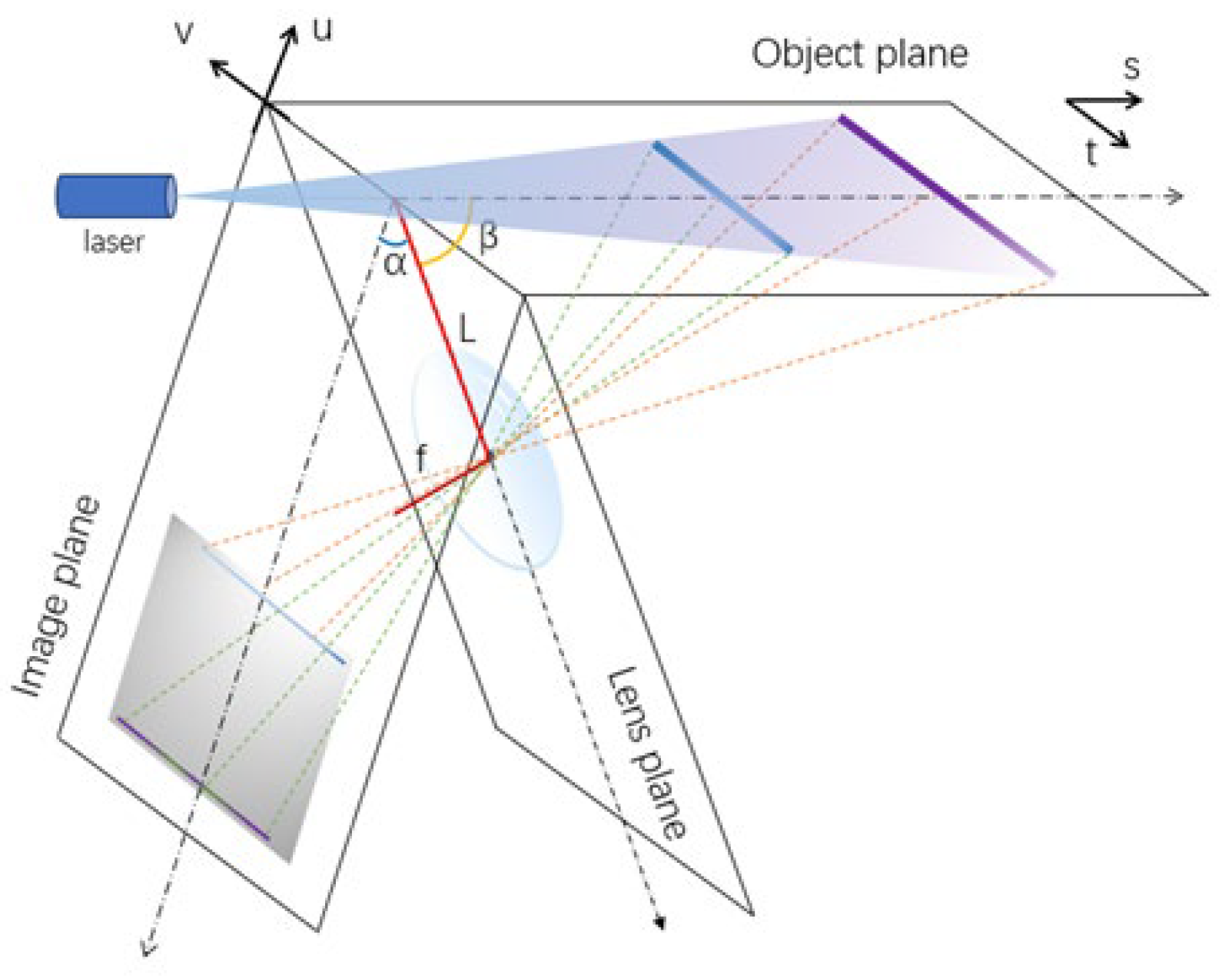
The proposed LiDAR is based on the Scheimpflug principle, which requires two things to achieve the infinite field of view: (1) the image plane, lens plane, and object plane should intersect in the same line; (2) the angle between the lens plane and image plane (α) as well as the angle between the object plane and lens plane (β) should satisfy Equation (1), which is derived from theoretical geometrical optics.

$$\alpha =\arctan \left({\displaystyle \frac{{\sin }^2\beta \cdot L}{\sin \beta \cdot \cos \beta \cdot L-f}}\right)$$

(1)

Here, L represents the distance between the center of the lens and the intersection line, and f represents the focal length of the lens.

When a light sheet is generated to illuminate the object plane, as shown in Figure 1, any substances on this plane will reflect the beam. The two-dimensional CMOS sensor would receive light reflected from different positions on the object plane through the lens, which concentrates it onto the corresponding pixels. The position of substances on the object plane (coordinates referred to as s and t) can be calculated from their positions on the image plane (coordinates referred to as u and v) through Equations (2) and (3). Therefore, the two-dimensional positioning of the target results in the advantage of accelerating the scanning efficiency by two or three orders compared with one-dimensional LiDAR.

$$s={\displaystyle \frac{u\cdot f\cdot \sin \alpha }{[u\cdot \sin \alpha -f]\cdot \sin \beta }}$$

(2)

$$t=-{\displaystyle \frac{f\cdot v}{u\cdot \sin \alpha -f}}$$

(3)

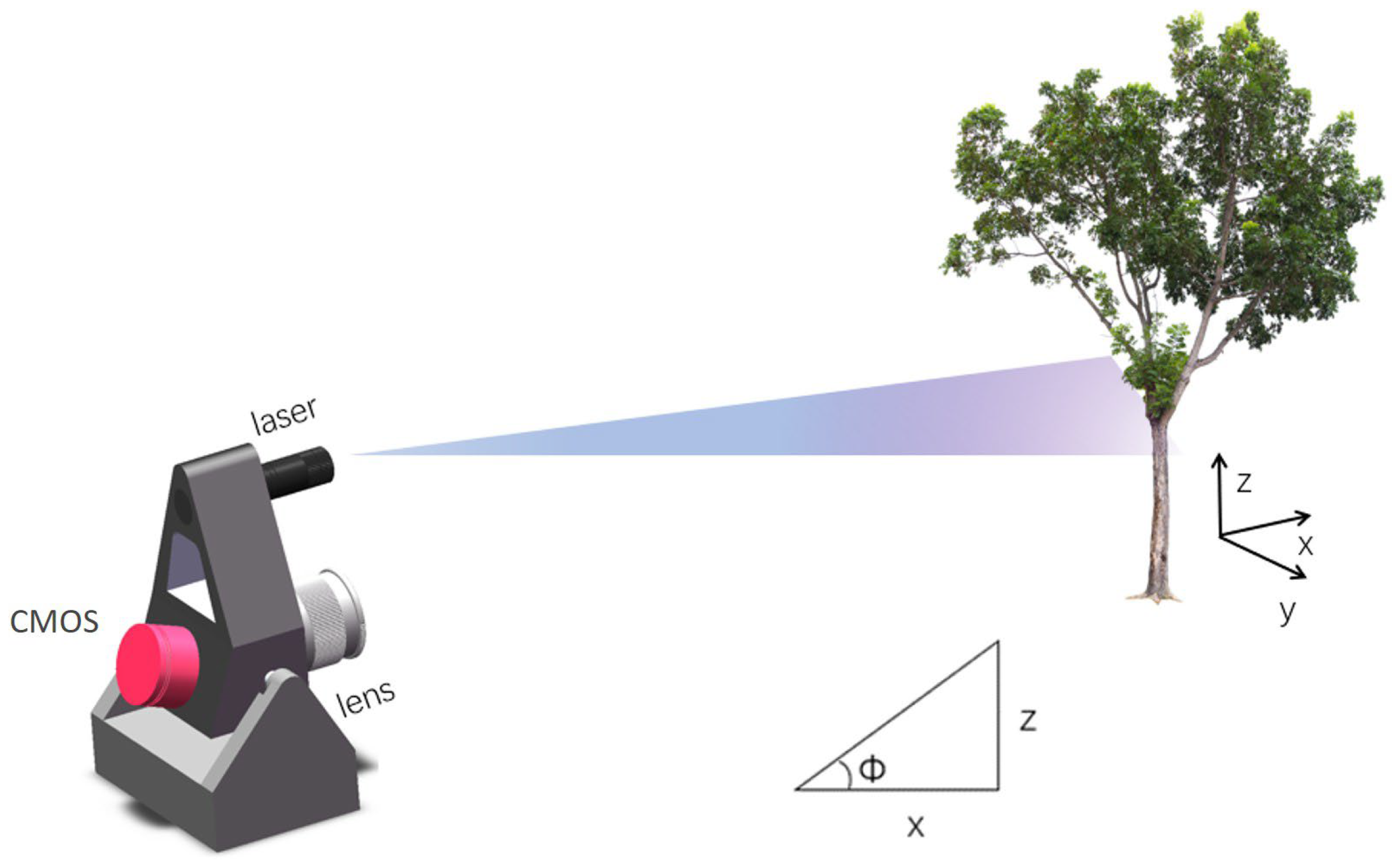
Figure 2 shows an illustrated view of the SLiDAR, which consists mainly of a laser module, a lens, and a CMOS image sensor. The laser module adopts a blue laser diode with a maximum optical output power of 1 W and a central wavelength of 445 nm. By mounting a Powell lens ahead, the module generates a light sheet with a divergence angle of around 45°. The lens (Canon, EF-S, Tokyo, Japan) supports a tuning focal length from 18 to 55 mm, and this time was fixed to 18 mm to obtain a wider field of view. The colorful CMOS (Panasonic, MN34230PLJ, Kadoma, Japan) has 4656 × 3520 pixels, each of a size of 3.8 × 3.8 µm. α is equal to 90°, and L is set to 10 cm. The SLiDAR system was mounted on a servo motor with a minimum rotation angle of 0.1° to enable the SLiDAR to scan within an elevation angle ranging from −30° to 70°. The rotation axis of the motor is parallel to the intersection line. Also, it is designed through the focal point of the lens. Based on this mechanical structure, coordinates in three-dimensional space (x, y, z) can be obtained through the successively obtained two-dimensional positions, their corresponding elevation angles (Ф), and trigonometry. The conversion of three-dimensional coordinates depending on the mechanical structure of the proposed LiDAR shown in Figure 2 is as follows:

$$x=s\cdot \cos \mathsf{\Phi }-L\cdot \sin \mathsf{\Phi }$$

(4)

$$y=t$$

(5)

$$z=s\cdot \sin \mathsf{\Phi }+L\cdot \cos \mathsf{\Phi }-L$$

(6)

The SLiDAR system is controlled by a self-built program based on Python version 3.11 to rotate the motor, modulate the laser, and obtain and record data automatically. A battery is equipped to facilitate field scanning.

2.2. Preprocessing

The preprocessing includes two aspects. The first aspect aims to increase the signal-to-noise ratio (SNR), which contains three steps, including background removal, threshold setting, and filtering. These steps can enable the instrument to obtain effective data even in the wild at night under the influence of environmental light.

Firstly, to reduce the impact of ambient light, scans are generally performed in dark environments, e.g., overcast or at night. However, reflections from bright sources such as street lights still have a significant impact on the subsequential spatial information retrieval process. This influence is eliminated by collecting the images at each elevation angle with the laser turned on and off, respectively, and deducting the background from the on image.

Secondly, a threshold was set to further increase the signal-to-noise ratio. Though very close in values for most pixels except for the region of the laser streaks, the background image and the target image are captured at close but different times, sometimes resulting in a small slow-fluctuating bias. Setting the values of any pixel smaller than the threshold to zero not only reduces this bias but also prevents random noises.

Thirdly, due to the complex surface morphology of plants, Gaussian filtering is applied to the original image data to smooth the intensity distribution of the original laser streak and remove a small amount of noise. The kernel size (k_size) of Gaussian filtering is approximate to the width of the light streak (σ) and is set according to Equation (7). The widths of light streaks exhibit distance-dependent variations, with broader patterns observed for proximal targets and narrower profiles associated with distant objects. This scaling relationship necessitates careful consideration when configuring k_size. Excessive k_size values may induce oversmoothing effects that compromise the preservation of fine structural details, particularly in distant targets. Empirical optimization in our experimental framework demonstrated that moderate kernel dimensions of (3, 3) or (5, 5) achieve the optimal balance between noise suppression and feature preservation.

$$k_{\mathrm{size}}<{\displaystyle \frac{\sigma }{\sqrt{3}}}$$

(7)

The second aspect is to address potential deviations in intrinsic parameters (notably effective focal length and tilt angle) arising from optical path variations and mechanical tolerances. Specifically, a multi-distance calibration protocol was implemented. Calibration targets were positioned at several discrete planes spanning the operational measurement range (up to 10 m). At each plane, the reference pixel coordinates were acquired. A nonlinear least-squares optimization algorithm was then applied to minimize the discrepancy between measured and theoretical pixel positions through iterative minimization.

2.3. Spatial Information Retrieval

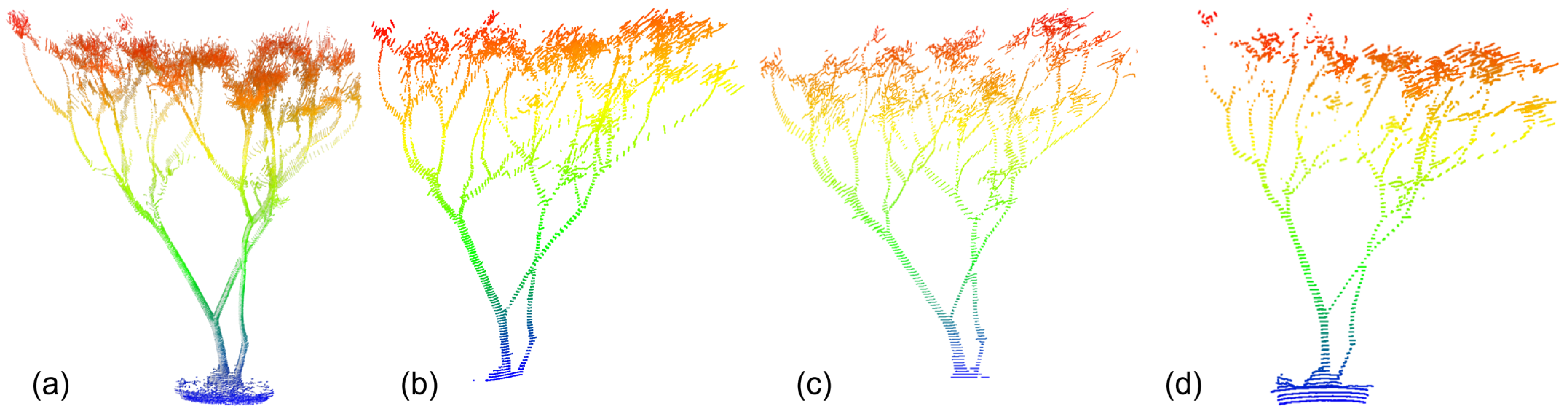
Three steps are involved for a SLiDAR to retrieve the point cloud of a target: (1) Obtain the position of the target on the figure obtained by the CMOS. As the light streak would expand due to the inhomogeneous of the light source, rough texture of the target, etc., methods are required to obtain the central positions of the signal. (2) Transform the central positions to two-dimensional positions on the light sheet plane according to Equations (2) and (3). (3) Transform the positions on the light sheet of each scan to spatial coordinates according to Equations (4)–(6). While the latter two steps are determined by the optical and mechanical structure, which is not tunable once the structure is established, the first step is optimizable. Here, four methods, i.e., the maximum method, center of gravity method, Steger method, and distance-adaptive Gaussian fitting method, are described and compared. Among them, the maximum method is the one employed in our previous works, as can be observed in [23,29,31], and this time it is considered as a baseline for position retrieval. The center of gravity method and Steger method are widely used in digital image processing, automated guided vehicles, etc. The Gaussian fitting method has been extensively used in full-waveform LiDAR; here, we fix it to the SLiDAR, as it is distance-square proportional and two-dimensional.

2.3.1. Maximum Method

The maximum method seeks the position of the maximum value of each column. If more than one maximum value exists in a single column, only the first one will be recorded. This method could locate the central position to pixel level.

2.3.2. Center of Gravity Method

The center of gravity (CG) approach is a powerful tool for locating distribution centers and has been widely used in the field of digital image processing [32]. Taking each column into consideration, the CG method treats the whole list as an object, and calculates its center of gravity according to Equation (8)

$$CG={\displaystyle \frac{{\displaystyle \sum P{V}_i}•i}{{\displaystyle \sum P{V}_i}}}$$

(8)

where PV represents the pixel value, i denotes the index of the on computing pixel, ranging from 1 to the total pixel number of the column.

2.3.3. Steger Method

The Steger method is a widely used method to extract curvilinear structures in a two-dimensional matrix [33]. It takes the surrounding values of each pixel to obtain the structure, and thus greatly improves the accuracy. The method mainly includes two steps. For the first step, the direction (n_x, n_y), which is perpendicular to the line, is calculated according to the Hessan matrix of pixels with values higher than a certain threshold. For the second step, a quadratic polynomial is used to determine whether the first directional derivative along (n_x, n_y) vanishes within the current pixel. This was achieved by inserting (t_nx, t_ny) into the Taylor polynomial, and setting its derivative to zero. Criteria are made to ensure the accuracy of the position.

2.3.4. Distance-Adaptive Gaussian Fitting Algorithm

Based on the broadening characteristic, a distance-adaptive Gaussian fitting method for position retrieval is proposed, which can also achieve sub-pixel matching of streak centers and improve the range resolution of the SLiDAR. The fitting is also carried out column by column. For each column, the data are fitted by a Gaussian distribution curve, as described in Equation (9), with varying parameters, a, σ, and μ, which represent the amplitude, standard deviation (SD), and central position, respectively.

$$G(x)={\displaystyle \frac{a}{\sqrt{2\pi }\sigma }}{e}^{-{\displaystyle \frac{{(x-\mu )}^2}{2{\sigma }^2}}}$$

(9)

The fitting performance is evaluated by the sum of squares of fitting residuals, as defined by Equation (10). When the sum of squares of fitting residuals reaches its minimum through gradient descent, the parameters are regarded as the optimal. Here, i represents the data index, y represents the list being fitted, N represents the length of the list.

$$\epsilon (a,\sigma ,\mu )={{\displaystyle \sum _{i=1}^N(y_{data}[i]-\frac{a}{\sqrt{2\pi }\sigma }\cdot \exp (-\frac{{(i-\mu )}^2}{2{\sigma }^2}))}}^2$$

(10)

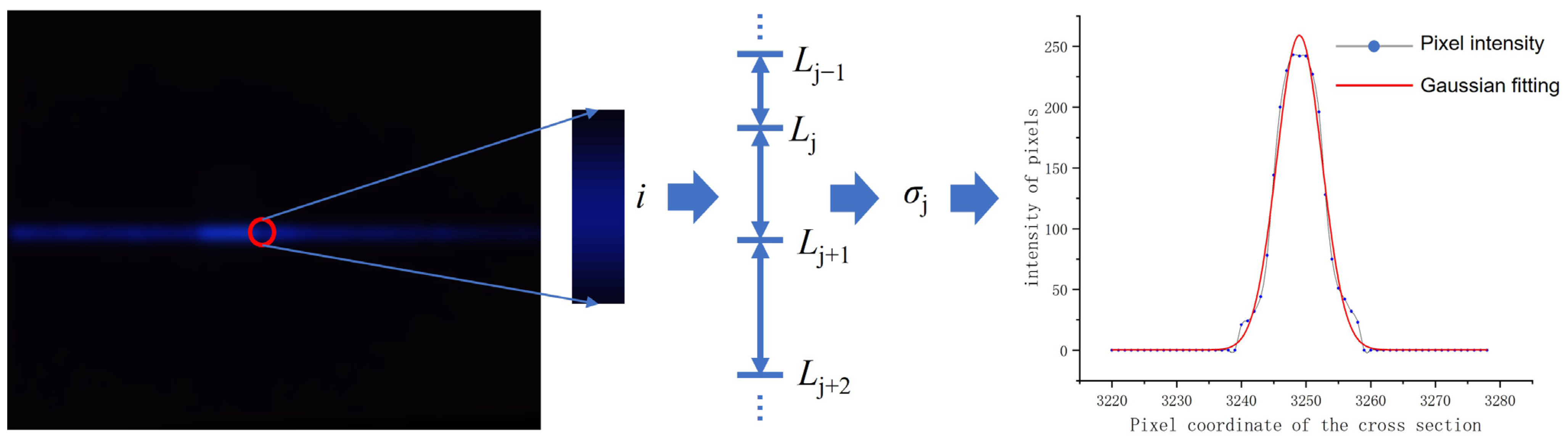
A close assumption of the initial parameter values would greatly accelerate the fitting process; thus, the maximum pixel value of each column is set as the amplitude, and its position is set as the central position. Referring to the SD, it is range-related. The signal coming from a near target has a larger SD, while that from a distant target has a smaller one. Meanwhile, the initial SD has a great impact on the fitting results: too small would lead to underfitting, reflecting that the point cloud is too discrete for distant points, making it difficult to capture the details of point cloud data changes; too large would lead to overfitting, which is more sensitive to noise and reduces robustness. To facilitate the Gaussian fitting for all distances, a distance-adaptive scheme is proposed. This time, the initial SD is not uniform along the detection range but set discretely between different intervals. In each interval, the initial SD set was examined in advance. As described in Equation (11), the total pixel position N is divided into m intervals; each starts from L_j, and ends with but not includes L_j+1. In each interval, a constant SD σ_j is set. To fit a curve with a central position at the ith pixel, the initial SD is set by firstly checking which interval performs i in, then picking the corresponding σ_j.

$${\sigma }_i={\sigma }_j i\in [L_j,L_{j+1}),j=1,2,\dots ,m$$

(11)

By adaptively selecting the appropriate initial SD using positional parameters, the best SD can be found within each measurable distance to optimize the fitting results. An example is shown in Figure 3 to show the process and its effectiveness.

2.4. Plant Height Calculation Method

Plant height is one of the most basic indicators in plant morphology research, defined as the distance from the base to the top of the plant. For the sake of uniformity, the direction perpendicular to the ground is selected as the z-axis, and the difference between the highest point of the plant and the highest point of the potted container along the z-axis is defined as the plant height [34]. The true heights of plant samples were measured using a ruler and compared with the results achieved from the point cloud.

2.5. Diameter Calculation Method

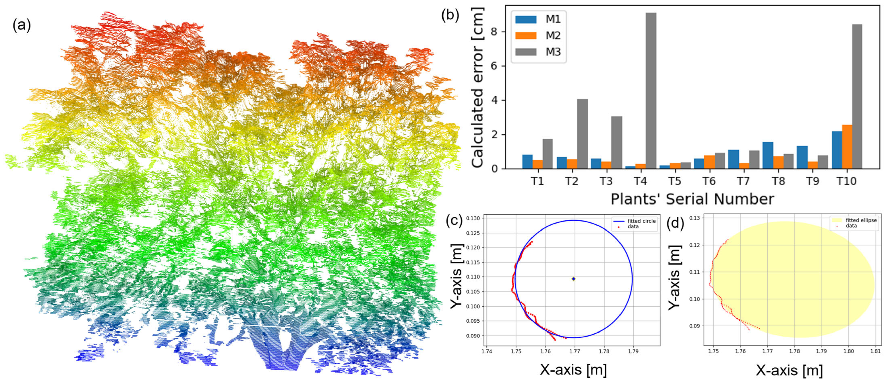
Plant stem diameter is also an important indicator in botany research and horticulture, providing information on plant growth and health status, species characteristics, maturity, etc. In order to reduce the error caused by irregular plant stems, slice data from the reconstructed single scan point cloud were intercepted in the z-direction to estimate the diameter. Three common methods were compared as follows:

• Calculating the maximum distance between two points as the diameter.
• Performing the minimum binary fitting circle on the data cloud, the diameter is achieved directly from the fitting circle.
• Similar to (b) but using an ellipse fitting instead. For an ellipse fitting, two axes are obtained, i.e., the major and minor axes. The perimeter of the ellipse is calculated, and the diameter is calculated from a circle of the same perimeter.

A vernier caliper was used to measure the true stem diameter of the plant samples and compared with the calculated results from the three methods.

3. Results

3.1. Spatial Accuracy Evaluation

To verify the effectiveness of the four spatial information retrieval methods, they were applied to the same sets of data. The data were acquired when the SLiDAR plane kept horizontal, and the laser module projected the light sheet perpendicular to a standard flat plate at distances of 1 m, 5 m, and 10 m, respectively, forming light streaks. The recorded data were preprocessed according to the methods described in Section 2.1, Section 2.2 and Section 2.3. Figure 4a shows the retrieved distances along the x-axis through the four methods at each distance. As can be seen, all four methods show good accuracy in the near field, i.e., 1 m, but the deviation increases along with the distance. For the target at 10 m away, the deviation is vivid, especially for the maximum method. The detailed SDs of the four methods at three distances are shown in

Table 1. Standard deviations of the four methods at three distances.

Method	SD (m) at Different Distances
	1 m	5 m	10 m
Gaussian	0.0004	0.0066	0.0440
Max	0.0012	0.0280	0.1787
Steger	0.0004	0.0074	0.0493
CG	0.0006	0.0095	0.0620

. The SD of the distance-adaptive Gaussian fitting method at different distances is the smallest among the four methods, indicating high precision. The behavior of the Steger method is close to the Gaussian fitting, while the maximum method shows an SD three times larger than the Gaussian fitting method at 1 m, and four times larger at the distance of 10 m. Although the Steger method can also reach sub-pixel level localization and achieves a similar SD level to the Gaussian fitting method, it may face line segment breakage and data loss caused by uneven streaks, as will be discussed below.

Figure 4b shows the retrieved two-dimensional point cloud of a tilt-placed box at a central distance of around 5 m. This placing method provides a vivid view for comparing the position retrieval ability of the four methods. The maximum method, which is only capable of locating the central point to pixel level, can only provide discrete positions. The CG, Steger, and Gaussian fitting methods could achieve sub-pixel level locating, facilitating the output line to be smoother. On the other hand, the CG method is more sensitive to noise, thus showing more fluctuations in the output line. On the left edge, the points determined by the Steger method spread, which is caused by the central line determination failure in the streak, as shown in the left insert of Figure 4b. The reason for this phenomenon is that the Steger method will apply calculation to pixels with values higher than a threshold. If the threshold is too small, many points would be included, and there will sometimes be more than one point in a column determined as the central point. Along the streak when determining the central line, some points are missing, as can be observed in the right insert of Figure 4b. In this case, the Steger method finds all calculated points shift more than half of a pixel, which means none of them would be regarded as the point of the central line. These phenomena can be reduced to some extent when raising the threshold. However, this could also block the recognition of the central line on the edges, where pixel values are often weak. The results coming from Gaussian fitting methods are decent, providing only one central point for each column on the edges.

3.2. Plant Height Measurement

To evaluate the ability of the SLiDAR to detect the height of plants, six Camellia sinensis (tea plants) were measured manually as well as through the SLiDAR. Plants were placed approximately 1.7 m away from the SLiDAR system. Scanning started at the angle where the light sheet covers the bottom of the container, with a rotation step of 0.1°. The height calculated is defined in Section 2.4 as the vertical distance between the highest points of the plant and the potted container. Figure 5a shows a real tea plant being scanned. The white streak is a light sheet, but too strong to show its original color when captured by camera. Figure 5b shows its point cloud achieved from a single scan of approximately 160 measurements of layers. A comparison was made between the true plant height measured manually, and the results from 3D point cloud reconstruction. It can be seen that the height error of the single-scan point cloud plant is no greater than 2.1 cm, as shown in Figure 5c.

To demonstrate the system’s adaptability to various distances and species, a rhododendron shrub plant was scanned at four different distances, i.e., 1.77 m, 2.9 m, 3.0 m, and 4.2 m. For consistent measurement, the bifurcation point at the base of each rhododendron was selected as the height reference, and the topmost leaf was selected as the terminal measurement point. The heights obtained from the point cloud for these four scans were 1.133 m, 1.107 m, 1.098 m, and 1.085 m, respectively, compared to the manual measurement of 1.135 m. The point clouds of the rhododendron shrubs are shown in Figure 6.

3.3. Diameter Detection

To evaluate the diameter-recovery ability of the three methods described in Section 2.5, a standard cylinder that has three segments of diameter was produced by 3D printing, as shown in Figure 7a. The diameters are 10 cm, 5 cm, and 2.2 cm, respectively, from the bottom to the top. It was scanned at a distance of 1 m, and its point cloud is shown in Figure 7b. The absolute values of calculated errors are shown in Figure 7c. In total, all three methods show good accuracy when calculating the circle point cloud, with errors of no more than 1 cm. Method 2 behaves the best for 10 cm and 5 cm diameters, showing an absolute error of less than 1 mm. For 2.2 cm diameter detection, Method 1 shows the best accuracy, followed by Methods 2 and 3. Overall, Method 2 is more accurate and robust for the diameter calculation of circular point clouds.

The three methods were also applied to calculate the stem diameters from the point clouds of the six tea plants (Figure 5b), rhododendron shrub (Figure 6a) at a distance of 1.7 m, as well as a Citrus medica L. at 2.9 m (Figure 8a). The results are shown in Figure 8b, where T1~T6 represent the six tea plants, T7 to T9 represent the diameters at 20 cm, 30 cm, and 40 cm of the right stem of the rhododendron shrub above the bifurcation point, and T10 measures the lowest 1.5 cm of the point cloud of the Citrus medica L. M1~M3 represent the diameter calculation methods described in Section 2.5. It can be observed that the diameters obtained by using the maximum distance (Method 1) and the least-squares method to fit the circle (Method 2) are in good agreement with the actual diameters, with calculated errors within 1 cm for T1 to T9. An example of Method 2 is given in Figure 8c, showing how circle fitting is applied to an irregular plant boundary. An example of Method 3 is also shown in Figure 8d, in which the point cloud is the same as in Figure 8c. This time, the ellipse is used to fit the point cloud, which is theoretically closer to the real shape of branches. However, when performing fitting, the major and minor axes of an ellipse are often mixed, leading the calculated error to several centimeters, as can be seen in T4 and T10.

4. Discussion

4.1. Trade-Off Between Detection Range and Field of View

Concerning the spatial ability of the SLiDAR, and of all kinds of LiDAR, two key parameters should be considered, i.e., the spatial accuracy as well as the detection range. For the time-of-flight LiDAR, typical parameters are ±3 cm in spatial resolution and up to 100 m in detection range, depending on the reflectivity of the target surface [10]. If the system is equipped with a high-speed data acquisition card and high-sensitive light detection module, e.g., avalanche photodiode (APD) or photomultiplier tube (PMT), a full-waveform LiDAR could be constructed reaching a resolution of several millimeters and a detection range of several kilometers [35], but the costs will be two orders of magnitude higher than the SLiDAR proposed. Based on the Scheimpflug principle, the spatial resolution of the SLiDAR is high in the near field, say within several meters, but low in the far field, say tens of meters. As for the detection range, it could be several kilometers when it is used for one-dimensional detection, as shown in the applications of aerosol detection [36]. But in our case, as it employs the two-dimensional scanning scheme to accelerate the scanning process, its detection range is decreased due to the weakness of the light strength caused by the divergence. To increase the detection range, a smaller divergence of the light sheet is required, which means a narrower field of view. A trade-off has to be made before the design of the SLiDAR, ensuring the target distance range in advance.

4.2. Influence of Ambient Light

The detection ability of the SLiDAR system is inherently coupled to the ambient light conditions, necessitating robust strategies to mitigate environmental interference. A core methodological innovation lies in the modulated laser pulse technique, which sequentially activates and deactivates the laser source to enable differential imaging via CMOS sensors, as described in Section 2.2. This approach effectively discriminates between laser-induced signals and ambient light artifacts.

Under low-light scenarios, extended exposure durations enhance the SNR, enabling reliable data acquisition. Nighttime or crepuscular operations are preferentially selected to minimize environmental light contamination, as these conditions inherently maximize the SNR. Conversely, high-illumination environments—such as midday measurements or scenarios with direct plant reflectance—pose significant challenges. Here, sensor saturation risks compromising reflection signal detection, particularly when sunlight overwhelms the laser-induced response. Mitigation strategies involve optical adjustments (e.g., restricted aperture diameters, reduced exposure times) to attenuate incoming light intensity. Moreover, the ratio of the target streak intensity to ambient light should remain ≥1. For instance, detecting a 2 m distant target generating a 2 m × 1 cm streak under irradiance levels (~50 W/m²) comparable to cloudy-day conditions demonstrates system adaptability.

4.3. Computation Time

Given that Gaussian fitting involves iterative optimization, the computational complexity is much higher than the other three methods. A comparison was made among the four methods on the data of the six tea plants, and the results are shown in

Table 2. Comparison of the computation time of the four methods on different tea plant samples.

Sample	Computation Time (s)
	Gauss	Max	CG	Steger
T1	499.697	11.229	15.011	197.674
T2	815.005	13.559	19.441	231.171
T3	843.992	13.513	19.770	242.462
T4	542.548	10.443	14.403	162.003
T5	1068.124	12.568	19.684	287.613
T6	628.395	11.656	16.117	183.074
Average	732.960	12.161	17.404	217.333

. The computational efficiency of the four methods exhibits significant disparities across the tested samples. The Max method demonstrates remarkable speed, with an average computation time of 12.161 s, making it the fastest algorithm in this comparison. The CG method follows closely with 17.404 s, offering a balanced trade-off between speed and potential robustness. These rapid performances suggest their suitability for real-time or large-scale data processing tasks where speed is critical, and accuracy is secondary. In contrast, the Steger method, averaging 217.333 s, and the Gauss method at 732.960 s, exhibit considerably longer computation times. The time consumption contributes to their improvement in accuracy.

4.4. Error in Height Measurement

Referring to the plant height measurement, as can be observed from Figure 6, the error progressively increased from 0.2 cm to 5 cm with distance. This error may be due to two primary factors: Firstly, with the increasing distance, the light intensity on the plant surfaces diminishes quadratically as the light sheet will not only expand fast along the so-called fast axis, but also slowly along the slow axis. Consequently, leaves at the periphery receive weaker illumination and exhibit shallower incident angles, causing their echo signals to be more easily removed by the threshold set in Section 2.2. Secondly, as the distance increases, each scanning step (0.1° in our case) covers a larger span according to trigonometry. This results in greater “height overshoot” during the final scanning layer, where portions of the plant’s upper structure are not fully captured, leading to underestimated height calculations.

4.5. Error in Diameter Detection

Referring to the diameter detection, the results in Figure 8b demonstrate that for circular/ellipsoidal stems, the circle fitting method consistently yields the lowest error margins across species. However, when measuring irregular stem structures such as the bifurcated region of Citrus medica L., all three methods exhibit increased error rates. Under these conditions, M1 demonstrates the smallest calculated error while M3 produces the largest calculated error. This finding suggests that M1 maintains superior robustness when assessing the diameters of irregular stems or branching structures.

4.6. Noise Raised by CMOS Sensor and Mechanical Rotation Accuracy

To evaluate CMOS sensor noise, ten repeated measurements of a target positioned 2 m away were conducted, yielding a standard deviation of 0.79 mm. This result highlights the inherent limitations of optical sensing systems, where noise originates from both sensor electronics and illumination fluctuations. Effective error mitigation strategies could involve adopting higher-precision power regulation for the laser, extending CMOS exposure durations, and optimizing the SNR through advanced signal processing.

Regarding the mechanical rotation accuracy, the critical limiting factor is the servo motor’s angular resolution. The current system employs a 15-bit encoder achieving ~0.011° theoretical resolution. This rotational precision directly translates to distance-dependent vertical positional errors. For example, at 2 m, this resolution corresponds to approximately 0.2 mm vertical error, which increases to 1 mm at 10 m. This error is acceptable compared to other error sources.

5. Conclusions

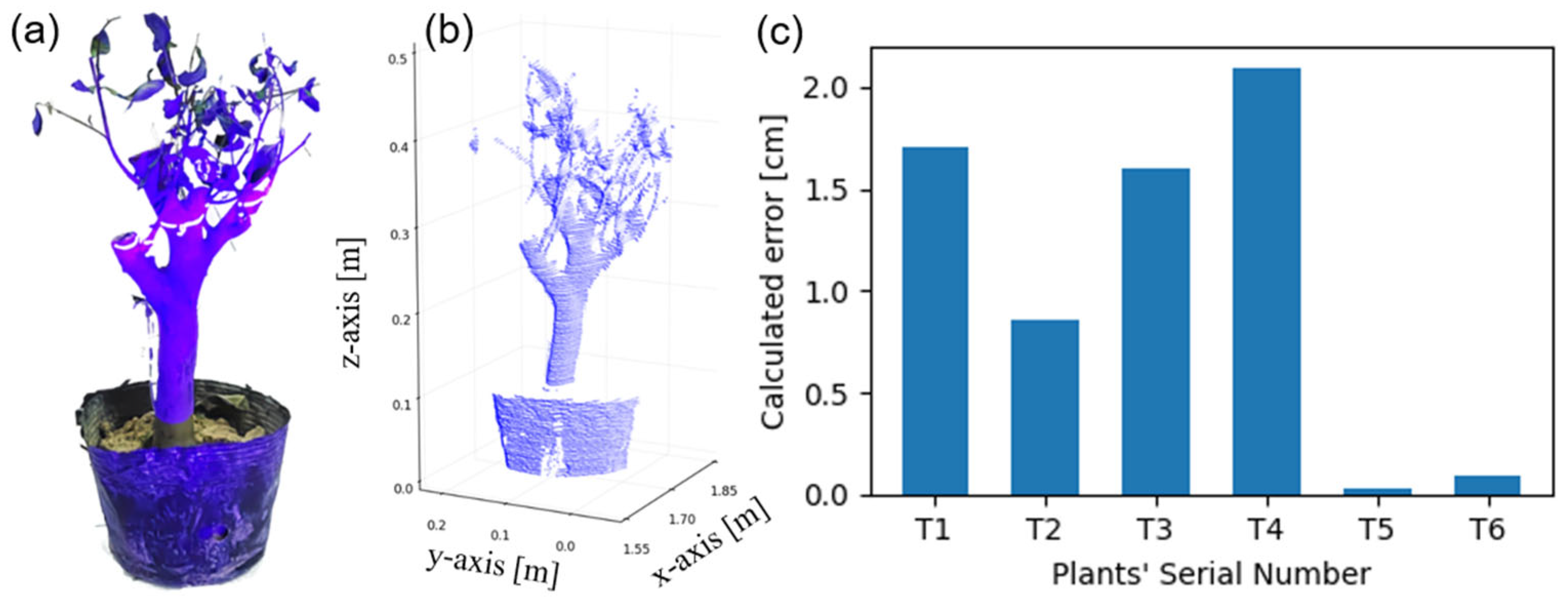
In conclusion, based on the proposed distance-adapted Gaussian fitting algorithm, the position retrieval accuracy is greatly improved. Spatial parameters such as the tree height and diameter are calculated from the single-scan point cloud, reaching errors less than 2.1 cm and 1.0 cm for plants of a height of around 0.5 m and a distance of 1.7 m, respectively. These results demonstrate the significant potential of the proposed SLiDAR in plant phenotypic measurement in real-world applications, especially for single-scan situations.

The future plan of the research is to try to perform a more precise calibration on the Slidar [37,38], and install the SLiDAR onto a drone, so that it can obtain the crown of trees as well as scan a larger area for point cloud detection. The aboveground biomass calculation, after getting rid of the points of leaves, will be performed and tested.