Unified Deep Learning Model for Global Prediction of Aboveground Biomass, Canopy Height, and Cover from High-Resolution, Multi-Sensor Satellite Imagery

Abstract

Regular measurement of carbon stock in the world’s forests is critical for carbon accounting and reporting under national and international climate initiatives and for scientific research but has been largely limited in scalability and temporal resolution due to a lack of ground-based assessments. Increasing efforts have been made to address these challenges by incorporating remotely sensed data. We present a new methodology that uses multi-sensor, multispectral imagery at a resolution of 10 m and a deep learning-based model that unifies the prediction of aboveground biomass density (AGBD), canopy height (CH), and canopy cover (CC), as well as uncertainty estimations for all three quantities. The model architecture is a custom Feature Pyramid Network consisting of an encoder, decoder, and multiple prediction heads, all based on convolutional neural networks. It is trained on millions of globally sampled GEDI-L2/L4 measurements. We validate the capability of the model by deploying it over the entire globe for the year 2023 as well as annually from 2016 to 2023 over selected areas. The model achieves a mean absolute error for AGBD (CH, CC) of 26.1 Mg/ha (3.7 m, 9.9%) and a root mean squared error of 50.6 Mg/ha (5.4 m, 15.8%) on a globally sampled test dataset, demonstrating a significant improvement over previously published results. We also report the model performance against independently collected ground measurements published in the literature, which show a high degree of correlation across varying conditions. We further show that our pre-trained model facilitates seamless transferability to other GEDI variables due to its multi-head architecture.

1. Introduction

The forests of the world are estimated to store up to 500 petagrams (Pg) of carbon in their aboveground biomass [1] and act as a major carbon sink, which is vital to maintaining stable ecosystems. According to the IPCC Sixth Assessment Report [2], deforestation and forest degradation contribute roughly 8–10% of global greenhouse gas emissions, accelerating climate change. Regular assessment of global aboveground carbon stock is essential for understanding and mitigating climate impacts, supporting corporate emissions disclosures, ensuring regulatory compliance, and contributing to international climate initiatives such as the UN Paris Agreement [3]. This poses an immense challenge, as it is the only validated and accurate method for both measuring tree profiles (including canopy height) and calibrating ecosystem-specific allometric equations.

Allowing the conversion of tree profiles into biomass requires labor-intensive field measurements. More efficient and scalable methods involve air- or spaceborne LiDAR instruments, which are capable of scanning tree profiles across large areas [4]. However, there is a trade-off between the density and resolution of such LiDAR maps and the spatial extent. For example, airborne LiDAR surveys can generate high-resolution maps due to the dense flight paths but are limited in the area that can be covered. Spaceborne instruments such as the Global Ecosystem Dynamics Investigation (GEDI) project [5] can cover the entire globe but their measurements are very sparse. In order to bridge the gap between dense estimation and global scalability, remotely sensed data, together with machine learning techniques, have become a main focus. Early approaches used simple ML methods, such as the random forest algorithm, resulting in pixel-wise estimation of canopy height on local scales [6] as well as low-resolution global canopy height maps (CHM) [7]. Recent methods have pushed the boundaries and generated higher-resolution maps, both of AGBD [8] and CH [9], by combining high-resolution imagery with various sources of LiDAR and ground measurements, as well as state-of-the-art computer vision models. Despite these advancements, there remain multiple challenges due to the availability of frequent, cloud-free observations of high-resolution satellites. In many cases, the imagery used spans a long and inconsistent time range, which complicates the ability to track changes in the carbon cycle. Moreover, many solutions achieve high accuracy for estimating AGBD or CH on regional scales but lack the ability to expand the model to the entire globe. The benefit of a single global model is learning from a diverse set of training samples across multiple ecosystems, resulting in a base model with good accuracy for broad-scale monitoring. Further fine-tuning of the base model locally can achieve greater accuracy with far less effort and cost than training multiple local models from scratch [10,11,12]. Especially when AGBD is determined using local allometric equations, the use of the base model accelerates the workflow and further reduces error metrics, as demonstrated in Section 4.3.

The detection of deforestation events requires the classification of land cover into forest, for which there are different definitions based on CH and CC [13]. Having estimates of both variables at a global scale allows for the application of different forest definitions dynamically and the detection of deforestation events by differentiation of binary maps at different times. In this work, we present a new approach that addresses many of the shortcomings mentioned above by introducing a deep learning-based model that unifies the prediction of AGBD, CH, and CC, as well as their uncertainties, into one single model trained on a global dataset of fused Sentinel-1, Sentinel-2, digital elevation model (DEM), and geographic location. We leverage the data from GEDI to generate sparse ground truth maps. Due to the spatial sparsity, we introduce a novel technique for training our model, which results in better performance compared with traditional methods. We show the results of the model deployment over the recent year (2023) at a global scale, as well as historic imagery back to the year 2016 in intervals of 1 year at a local scale. 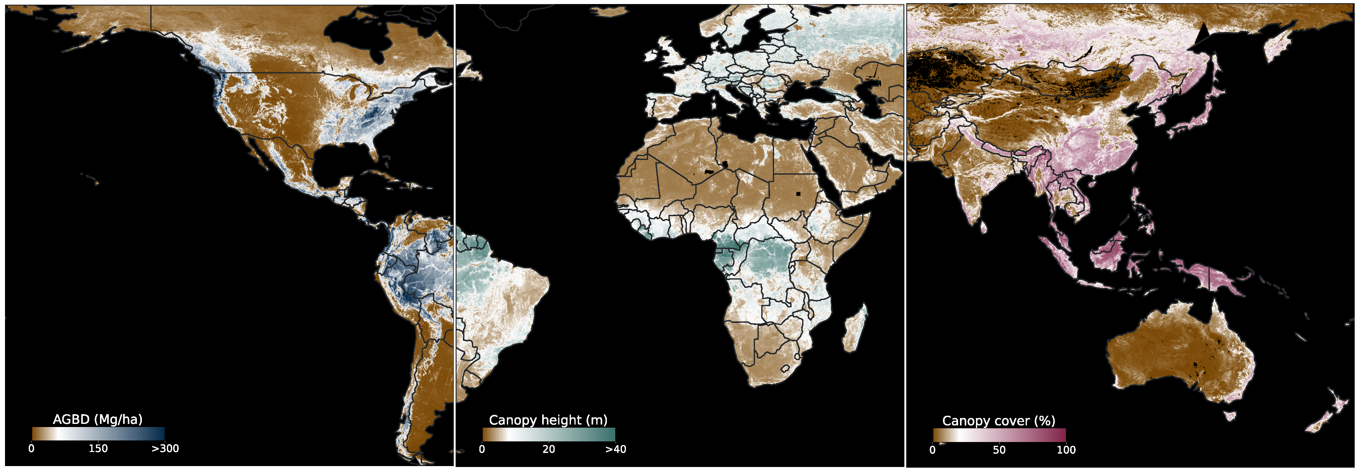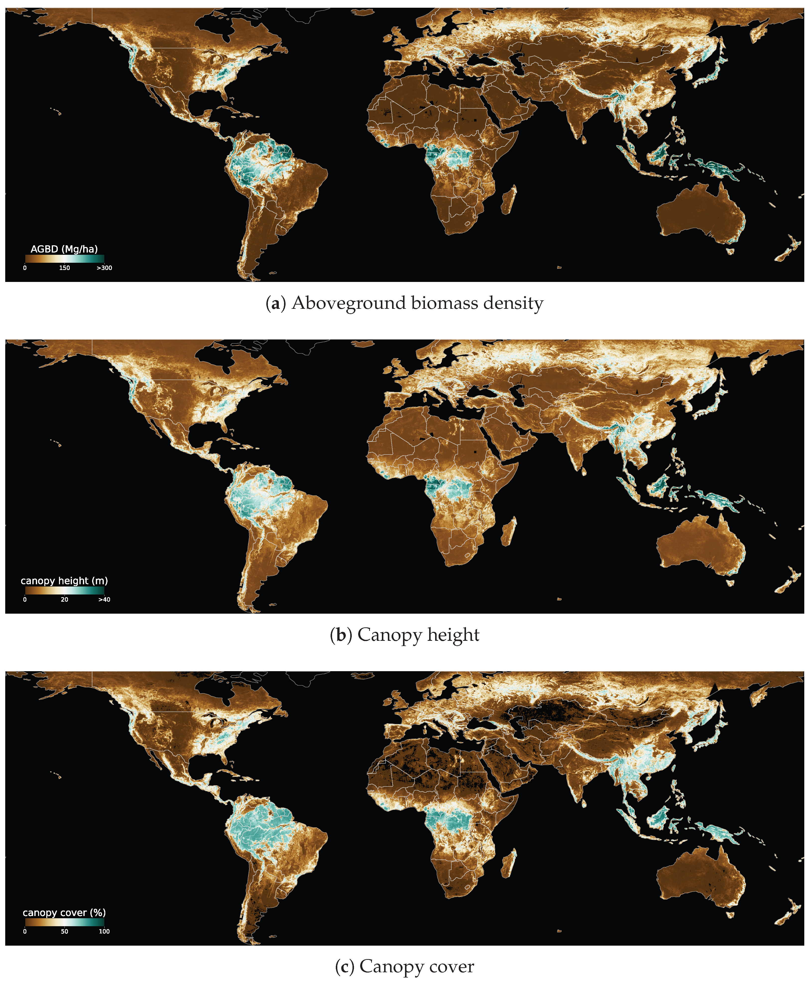Figure 1 shows a composition of global ABGD, CH and CC maps generated in this study.

The generated dataset for the training of the deep learning model consists of ∼1 M training and ∼60 k validation samples composed of cloud-free image tiles of size 256 pixels × 256 pixels at 10 m ground distance.

Previous work: Over the past two decades, increasing focus and effort have been directed to environmental monitoring based on spaceborne earth observation missions. Such missions go as far back as the 1970s with the Landsat [14] constellation, which offers an immense archive of medium-resolution satellite imagery. In recent years, specialized missions have paved the way for more accurate insights into the global dynamics of environments with higher revisit rates and resolution, including multispectral passive sensors [15,16,17,18], active sensors such as synthetic aperture radar (SAR) [19,20], light detection and ranging (LiDAR) [5], and missions dedicated to understanding the carbon cycle [21,22]. The increasing volume of data collected by all these missions has motivated the development of modern and novel algorithms based on machine learning and deep learning [23]. Previous work has focused on the model development for estimating either aboveground biomass density, canopy height, or canopy cover. We could not find any references that combine the prediction of multiple variables into a single model. In most previous approaches, the limitation in spatial resolution arises from the choice of input data source and ranges from 250 m–1 km (e.g., MODIS) to 30 m (e.g., Landsat), 10 m (e.g., Sentinel-1/2), and ∼1 m (e.g., MAXAR).

Biomass: Aboveground biomass maps are available today, covering up to decades of history, but are often produced on a local scale based on ground measurements and forest inventories [24]. Scaling these maps to larger regions requires the collection of plot data, which covers various ecosystems. Capturing ground-truth data across the broad range of ecosystems and land cover that would be required to scale this methodology would be prohibitively expensive. Early efforts incorporating simple machine learning techniques have focused on pantropical regions and use medium-to-low resolution satellite imagery [25,26,27]. At a global scale, a number of aboveground biomass maps have been generated at low resolution (∼1 km) [28,29], including the gridded version of the GEDI level 4 product [30]. Only recently, with the incorporation of modern deep learning techniques, have higher-resolution maps emerged [8,31], which combine the use of satellite imagery with global-scale LiDAR surveys.

Canopy height: Unlike aboveground biomass, canopy height estimates from satellite imagery are less dependent on regional calibrations, as ground measurements can be gathered directly from forest inventories or LiDAR measurements that provide information on canopy structure. Early approaches utilize simple pixel-to-pixel machine learning algorithms, such as random forest, at medium resolution [7,32], while more recent methodologies were developed based on deep learning models and higher resolution and single-sensor imagery [33], as well as combining multiple sensors as input data [9]. Advances in deep learning-based computer vision models, which exhibit great depth estimation skills [34], have allowed the development of very high-resolution canopy height maps [35] and models that characterize single trees [36,37,38]. The main drawback of very high-resolution maps at a global scale is the immense computational effort and cost for a single deployment. In order to cover the entire globe, high-resolution imagery is often gathered within a large time window (multiple years), which creates an inconsistency in the temporal resolution and complicates the change monitoring. In order to create consistent and high-quality global maps, it is therefore advisable to revert to lower-resolution imagery (∼10 m) with a higher frequency of observations and to merge multiple sources that may complement each other. Large-scale LiDAR surveys provide a more direct way of generating canopy height maps since they do not rely on models that estimate canopy height based on imagery, which has limitations in information content. However, high-resolution aerial surveys [39] are limited in scalability, while global-scale surveys have low resolution [40].

Canopy cover: Estimating canopy cover from satellite imagery is the least complex of the three tasks, as it does not rely on a detailed three-dimensional canopy structure or local calibrations. However, it may still pose many challenges due to the quality and resolution of the input imagery. The first global canopy cover maps based on remote sensing are derived from Landsat imagery at medium resolution [41]. Different satellite sources at varying resolutions have been used in generating regional maps [42,43], while historical imagery, despite the low resolution, allows high-frequency updates reaching back many decades [44].

To the best of our knowledge, our work is the first to combine the estimation of aboveground biomass density, canopy height, and canopy cover into a single unified model. With respect to single-variable estimation, our approach is most similar to [8] for aboveground biomass density and [9] for canopy height, to which we compare our model evaluation results (see Section 3). In summary, the main contributions of this work are as follows:

• First deep learning-based model that unifies the prediction of aboveground biomass density, canopy height, and canopy cover, as well as their respective uncertainties.
• Advancements for predicting global-scale maps at high resolution at regular time intervals without missing data due to multi-sensor fusion.
• Novel training procedure for sparse ground truth labels.
• Extensive evaluation against third-party datasets as well as a demonstration of model fine-tuning for local conditions.

2. Data and Methods

In this work, we use multispectral, multisource satellite imagery, a digital elevation model, and geographic coordinates as input to the model. The model is trained in a weakly supervised manner (see Section 2.3) on point data from the Global Ecosystem Dynamics Investigation (GEDI) instrument. In this section, we describe the processing steps for generating a global dataset of input and target samples. We will also briefly explain the relevant concepts of the GEDI mission as well as the different data processing levels, as this will be an important aspect of understanding the inherent uncertainties of the model and its limitations.

2.1. Ground Truth Data

The GEDI instrument is a spaceborne LiDAR experiment mounted on the International Space Station (ISS) and has been operational since 2019. It comprises 3 Nd:YAG lasers, optics, and receiver technology, allowing it to measure the elevation profile along the orbital track of the ISS. Within the lifetime of the experiment, it is expected to collect 10 billion waveforms at a footprint resolution of 25 m. The setup of 3 lasers, one of which is split into two beams, as well as dithering every second shot, leads to a pattern of point measurements with 8 tracks per pass where the tracks are separated by 600 m and each point by 60 m along the flight path. Each GEDI measurement consists of the waveform resulting from the returned signal of the laser pulse sent out at the given location. The collection of all these waveforms is referred to as level 1 data. Each waveform is further processed to extract metrics that characterize the vertical profile of trees within a given beam footprint.

The signal with the longest time of flight corresponds to the ground return and is used as the reference for the relative height (RH) metrics. The RH[X] metrics correspond to the relative height at which [X] percent of the total accumulated energy is returned. These metrics characterize the vertical profile of the GEDI footprint, where RH100 corresponds to the largest trees in the footprint. These metrics, together with other parameters related to the measurement conditions, are stored in a dataset referred to as level 2a. In additional steps, these metrics are used to calculate the percent canopy coverage (level 2b), as well as a gridded version (level 3). Further processing involving regional calibration of allometric equations, using level 2 data, results in estimations of aboveground biomass density (AGBD) as well as uncertainties referred to as level 4a. Estimates are based on models that were fitted to biomass measurements on the ground in a number of field plots located in various regions around the world. Since most of these measurements do not intersect with a GEDI footprint, airborne LiDAR was used to measure the return signal, which was then translated into a simulated GEDI waveform. In this work, we use the level 2a/b and level 4a data as ground truth. The on-the-ground measurements for biomass were mostly done without any tree clearing but by measuring canopy height and diameter and using allometric equations specific to the tree type and the world region to determine biomass. The simulated waveforms undergo the same processing to extract RH metrics, which provide the predictors for linear models to predict AGBD. Various models were developed for all combinations of plant functional type (PFT) and world region defined as the prediction stratum. For details of the selected predictors for each model and their performances, see Sections 1 and 2 of [45].

The models are linear functions of the predictors with a general form of

$$f_j=X_j{b}_j$$

(1)

where $X_j$ is a $n\times m$ matrix of n measurements with m predictors and $b_j$ a $m\times 1$ vector of parameters for prediction stratum j. The best parameters are determined by linear regression, where the predicted variable may be in transformed units using a function h, which is either unity, square root, or log. For new measurements $X^{\prime }$, the model of the corresponding prediction stratum is chosen, and the predictions are given by

$$AGBD=h^{-1}\left(X^{\prime }b+ϵ\right)$$

(2)

where $ϵ$ is a bias term determined by the fit residuals in the respective prediction stratum. For each prediction of footprint k, a standard error is calculated, which is defined as

$$S{E}_k=\sqrt{MS{E}_j+X_{k}cov\left(b\right)X_k^T}$$

(3)

as well as a confidence interval given by

$$AGBD\pm t\left(1-{\displaystyle \frac{\alpha }{2}},n-2\right)·S{E}_k$$

(4)

where t is the value of the t-distribution with n-2 degrees of freedom at a confidence level of $\alpha$. In general, we observe that the uncertainty on AGBD from the GEDI ground truth increases with the value of AGBD, where the main contribution comes from the residuals in Equation (3). This is an important fact to consider when training the model. During model optimization, it is generally assumed that the target values are the absolute truth, while in this case, we know that the target values are inherently uncertain. This means that a given input X can be assigned to two different values, $Y_1$ and $Y_2$, which cannot be described by a continuous function. Since only continuous activation functions are used in our CNN, the function it represents will also be continuous, which may lead to predictions with larger uncertainties or under-prediction in regions where the ground truth data are uncertain. We will discuss this in more detail in Section 3 and Appendix B.2. The largest ground truth uncertainty is introduced when converting canopy height, or generally RH metrics, to AGBD, which is more accentuated by the lack of ground plot measurements used for calibration. Our model provides an important benefit by not just predicting AGBD in an end-to-end setup but at the same time also predicting canopy height, which can be used for recalculating AGBD a posteriori should more accurate plot data become available.

The multi-head architecture of our model (see Section 2.3) allows for simultaneous prediction of multiple GEDI variables. For the training of the base model, we choose AGBD from level 4a, CH from level 2a, and CC from level 2b as the prediction variables. In Section 4.3 we demonstrate how the base model can be easily fine-tuned on different variables in the GEDI dataset. The level 2a dataset provides relative height metrics at discrete energy return quantiles from 0 to 100 in steps of 1, denoted RH00, RH01, …, RH99, RH100. It is common to choose one of RH95, RH98, or RH100 to define CH. Our base model uses RH98, which prevents over-prediction in cases where there are a single or a few very large trees among smaller trees. We save all RH metrics in our datasets so that they can be dynamically selected during training. This provides the flexibility to fine-tune the model on a different RH metric, or multiple RH metrics, depending on the requirement of local allometric equations.

2.2. Input Data

In order to leverage the respective benefits of different data sources, we fuse optical bands (red, green, blue) from the Sentinel-2 [46] satellite with thermal bands (nir, swir1, swir2) from the same satellite (processed with the SEN2COR algorithm [47] to provide surface reflectance) and synthetic aperture radar (SAR) signal (VV and VH backscatter) from Sentinel-1 [48]. In addition, we used altitude, aspect, and slope from the Shuttle Radar Topography Mission (SRTM) [49] to further enrich the predictive capability of our model. The predictors of the digital elevation model (DEM) carry important information about the local topography that affects the distribution of plant functional types and their growth patterns [50]. We also provide the global coordinates of each data sample by encoding longitude and latitude in the interval [−1, 1]. The optical bands of Sentinel-2 and the Sentinel-1 bands have a native resolution of 10 m, while the thermal bands of Sentinel-2 have a resolution of 20 m and the DEM of 30 m. In order for the CNN to process the input layers at different resolutions, we resample all layers to 10 m resolution using the bilinear interpolation method and stack them to form a 13-channel input tensor.

To generate a global training and test dataset, we uniformly sample locations within the latitude (longitude) range of [−51.6, 51.6] degrees ([−180, 180] degrees) that intersect with the landmass. We use the Descartes Labs (DL) proprietary tiling system to create image tiles of size 512 pixels × 512 pixels at 10 m/pixel resolution with the sampled coordinate being at the center of the tile. (Descartes Labs was acquired by EarthDaily Analytics after this work came out. Throughout this work, we will refer to any component of the DL system by its original name). Each tile is required to contain >20 GEDI footprints. During training, we dynamically split each tile into 4 non-overlapping sub-tiles of size 256 pixels × 256 pixels, which increases the total number of samples in the dataset four times. We introduce a naming convention for tiles based on their location in the southern hemisphere (lat < −23.5°), the tropics (−23.5° ≤ lat ≥ 23.5°) or the northern hemisphere (lat > 23.5°).

2.2.1. Cloud Mask and Image Composite

In order to reduce cloud obstruction and cloud shadows in Sentinel-2 imagery, we generate cloud-free composites from a stack of images that are masked with the binary output of our proprietary cloud and cloud shadow detection model. The cloudmask model is a UNet [51]-type architecture trained on ∼4.4 k ground truth samples collected globally and labeled by human annotators. The input to the model is the six-band Sentinel-2 imagery, while the target mask consists of three classes (cloud, cloud shadow, and background) for each pixel. The image stack is built by collecting all Sentinel-2 scenes that intersect with the given tile within a specified time range. Scenes taken on the same day are mosaiced. We used the median operation to generate the composite from the masked image stack. The composite time range is chosen to minimize the variability in the spectral response of the vegetation while maximizing the resulting coverage. We, therefore, chose the time ranges to be the respective summer months for the two hemispheres (June–August for the northern hemisphere and December–February for the southern hemisphere), except for the tropical region, where the composite was done over a 6-month period. In certain tropical regions, cloud artifacts are visible despite the long composite time range. This highlights the importance of multisensor fusion, where Sentinel-1 backscatter provides valuable information for these gaps since SAR is not affected by clouds. In order to reduce the noise in the SAR backscatter signal, we apply the same compositing method to the VV and VH bands without the cloud mask. In Section 2.5 we will discuss in detail the model performance in challenging regions with imperfect cloud-free composites.

2.2.2. Global Dataset

For each sampled tile, we generate Sentinel-1 and Sentinel-2 composites according to the definition in Section 2.2.1 by gathering imagery using the Descartes Labs platform for the year 2021 (2021/2022 for the southern hemisphere). The DEM has a fixed acquisition year of 2000. For a given tile, we gather all the GEDI level 2a/b and level 4a point data that lie within the geometry of the tile and have a collection date of no more than ±1 month from the composite time range (this buffer is set to 0 months for the 6-month composites). In order to match the data from GEDI level 2a/b with level 4a, they are required to have the same footprint coordinates to 5 decimal point precision and the same acquisition date. Furthermore, we only accept data with the quality flag l4_quality_flag equal to 1 and require that at least 20 data points be within the tile geometry. Due to the sparsity of the GEDI data, it is saved as vector data along with each footprint pixel coordinate and rasterized on the fly during training. Despite the footprint being 25 m in diameter, we assign the corresponding target value to only one pixel of size 10 m × 10 m at the location of the footprint center.

In total, 276,766 data samples were created, of which 14,745 (5%) were randomly selected and stored as a test dataset. Each sample is composed of an average of 50 scenes in Sentinel-1 and Sentinel-2, which is a total of 13.8 M scenes processed. The total number of ground truth data points is 67 M (3.8 M) for the training (test) dataset.

2.3. Model Development

The GEDI dataset offers measurements of AGBD, CH, and CC for recent years but is largely incomplete at higher resolution due to its sparsity. Here we describe the computer vision (CV) model we developed. It fuses selected bands of multiple sensors as well as encoded geographic location, forming a 13-channel image stack, to predict AGBD, CH, and CC as a continuous map at the resolution of the input source while using the GEDI level 2 and level 4 datasets for training.

In this work, we use the surface-level processed Sentinel-2 with six bands (red, green, blue, nir, swir1, swir2), the Sentinel-1 backscatter signal (bands VV and VH), and altitude, aspect, and slope provided by the digital elevation model from the SRTM mission at a resolution of 10 m. The choice of Sentinel as an input source is motivated by its global coverage, the relatively high spatial and temporal resolution, and the fact that the image collection goes back to 2016, allowing the deployment of the model on historical data.

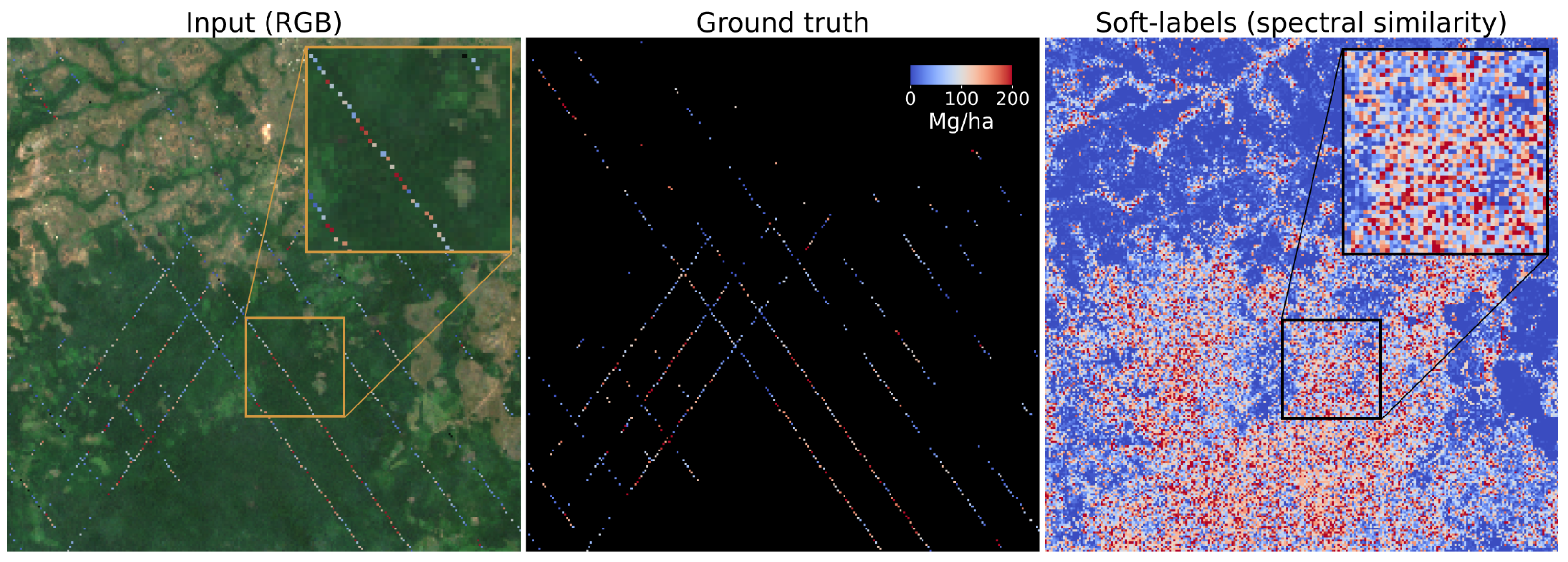
In Figure 2, a sample input image (RGB) and the corresponding AGBD ground truth data are shown. It illustrates the sparsity of ground-truth measurements and the need for a model that can fill in the gaps.

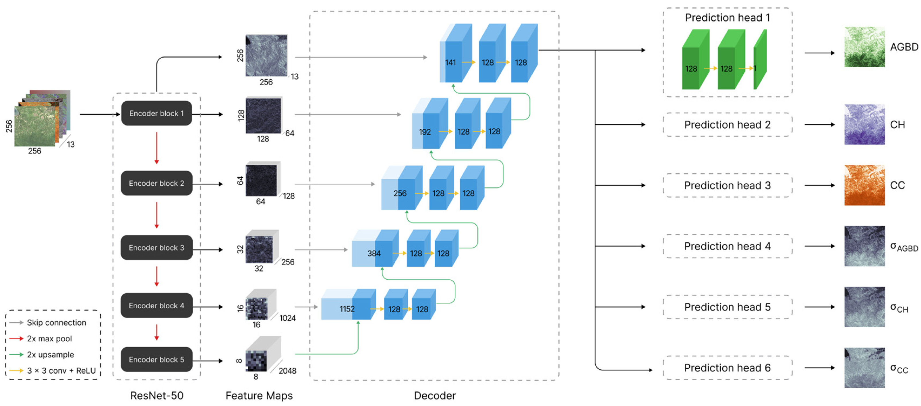
Our model consists of a convolutional neural network (CNN) [52] with three main components: an encoder network that extracts features from the input image, a decoder that processes the extracted feature maps at different depths of the network, and, together with the encoder, forms a feature pyramid network (FPN). The final feature map then consists of all the relevant information required for the estimation of the output variables. The final components are a set of prediction heads, which have the function of generating the estimate of each respective output variable based on the last feature map of the FPN. Each prediction head consists of a series of 1 × 1 convolutions. The encoder network can be any commonly used feature extractor. In this work, we chose ResNet-50 [53] as the encoder. The FPN consists of decoder blocks where each block takes the features of level $l-1$ and l as input. The feature map of level $l-1$ is up-sampled using a bilinear interpolation method and a convolution layer with kernel size 2 × 2 before concatenating with the feature map of level l, followed by two convolution layers with kernel size 3 × 3. The resulting feature map is then fed to the level $l+1$ decoder block until it reaches the final level corresponding to the input resolution. All convolution layers in the decoder have a fixed feature dimension of 128. Each prediction head consists of a series of 3 1 × 1 convolutions with feature dimensions [128, 128, 1]. All layers in the decoder and prediction heads use the ReLU [54] activation function except for the final layer of the prediction heads, which estimates the variable uncertainty for which we use the softplus [55] activation function. The weights of the entire network are randomly initialized using the Glorot Uniform [56] initializer. Figure 3 illustrates the model architecture with its various components. The total number of trainable parameters is 28.71 million.

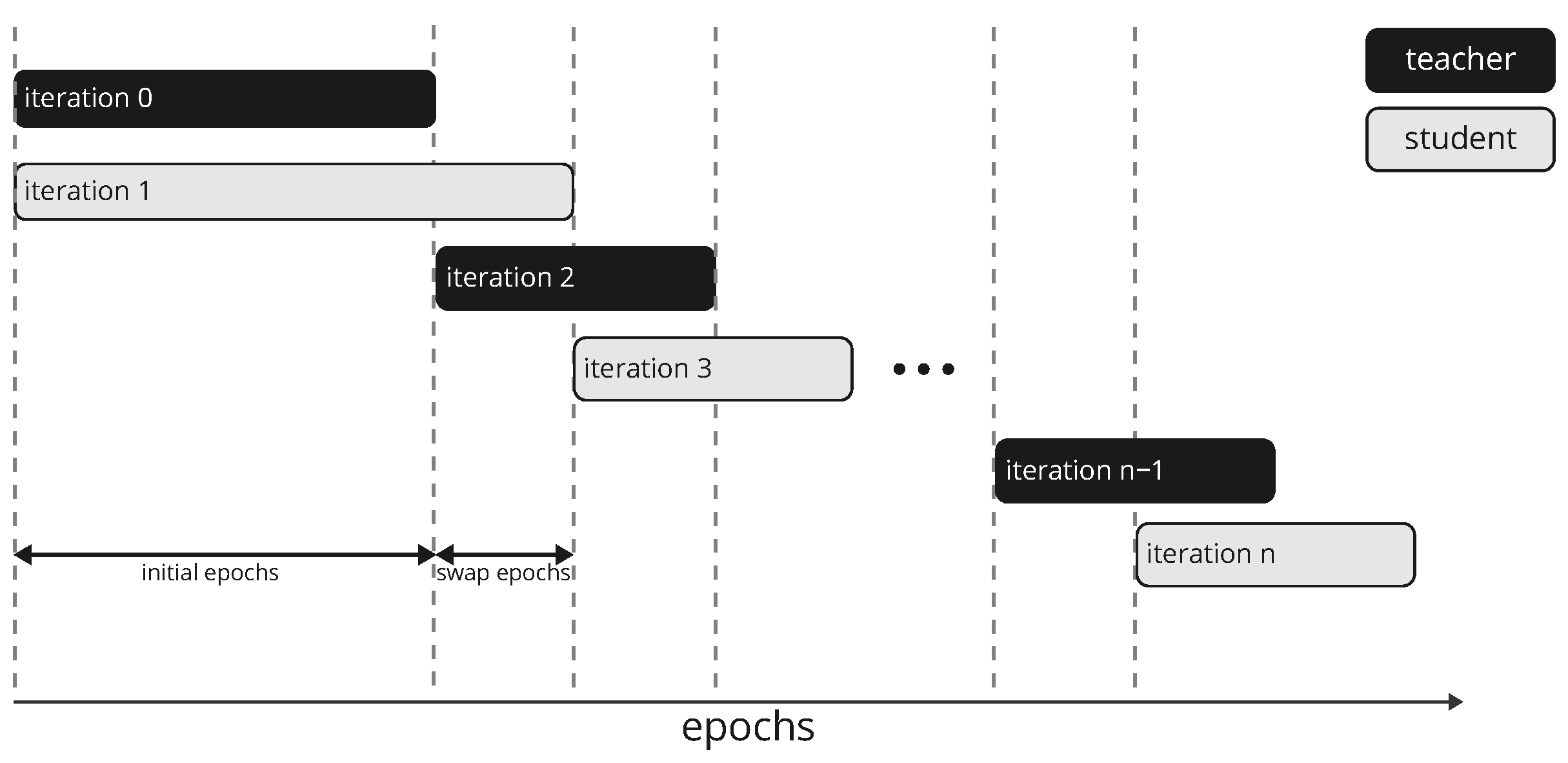
This model architecture generates an output map of the same size as the input image. In most cases of such a configuration, the target is expected to be a continuous map of the same size as the output from which the loss is calculated. In our case, the target is not continuous but is composed of sparse target values. A straightforward solution for this situation is to only evaluate the loss function at pixels for which a ground truth value is available. However, we found that this approach results in overfitting on the sparse pixels and generates a nonhomogeneous output. We, therefore, propose a new approach where we generate a continuous target map by a model acting as the teacher to a student network during the training process. This approach is similar to the student–teacher setup for classification tasks where ground-truth labels are incomplete. We extend this approach to dense regression tasks, as in this work. To begin with, we construct two identical networks in terms of the architecture whose weights are initialized separately and referred to as teacher (${\mathcal{F}}_T$) and student (${\mathcal{F}}_S$) networks. The task of ${\mathcal{F}}_T$ is to generate a continuous ground truth map from the input and the ground truth labels. ${\mathcal{F}}_S$ is then trained on this ground truth map. After a certain number of epochs, ${\mathcal{F}}_T$ and ${\mathcal{F}}_S$ swap their roles. This procedure is repeated until the two networks converge. Since both networks are randomly initialized, they are not very skilled during the initial training phase, and ${\mathcal{F}}_T$ cannot provide meaningful ground-truth guesses. We therefore replace ${\mathcal{F}}_T$ with a simple model based on spectral similarity at the input level during the first training phase of ${\mathcal{F}}_S$. We define the spectral similarity as the cosine similarity

$$\sigma \left(X_i,X_j\right)={\displaystyle \frac{X_i·X_j}{\parallel X_i\parallel \parallel X_j\parallel }}$$

(5)

where $X_i$ and $X_j$ are the vectors with spectral information of a set of bands for pixels i and j. The set of bands can be a combination of any of the available input bands. However, we find that this approach works best with a feature vector composed of the six bands of Sentinel-2.

For each pixel without a label, we compute $\sigma \left(X_i,X_j\right)$ with respect to all pixels that have a label (hard labels). We then assign the value of the hard label for which $\sigma \left(X_i,X_j\right)$ is maximal to the pixel without a label to generate a soft label. The target map is then a combination of hard and soft labels defined as

$$\widehat{y}=m\otimes \widehat{y_h}+(1-m)\otimes \widehat{y_s}$$

(6)

where m is a mask for which $m_{i,j}=1$ if pixel $i,j$ is a hard label and $m_{i,j}=0$ otherwise. Here, ⊗ denotes the element-wise product. Soft labels can be efficiently calculated for all unlabeled pixels by arranging them in a matrix A of size $n\times b$ and all hard label pixels in a matrix B of size $m\times b$, with b the number of bands. The soft labels are then calculated by

$${\mathrm{label}}_{idx}=\mathrm{argmax}\left(\widehat{A}{\widehat{B}}^T\right)$$

(7)

where $\widehat{A}$ and $\widehat{B}$ are the row-normalized matrices of A and B. Figure 2 (right) shows the result of this operation on the input shown in Figure 2 (left).

Here we use a simple model to generate soft labels according to Equation (5), which are good prior guesses for pixels with no target values in the first iteration of training ${\mathcal{F}}_S$. After the first iteration (initial epochs), ${\mathcal{F}}_S$ has acquired some skills to predict the target map and becomes the teacher for the second network, which is trained from scratch. The teacher network replaces the simple model for soft label generation based on spectral similarity, as it has inherent quality limitations due to noise. In order for the new student network to overcome the skills of the teacher network, the hard labels will be given more weight than the soft labels in the definition of the loss function (see Equation (12)), and ${\mathcal{F}}_S$ is trained for 8 more epochs (swap epochs) in the current iteration than ${\mathcal{F}}_T$ in the previous iteration. This procedure is illustrated in Figure 4. The soft labels generated by ${\mathcal{F}}_T$ are guesses and help guide network training, particularly in the early training phase, but may deviate from the actual ground truth label. We, therefore, use a weight schedule for the soft labels incorporated into the loss function (see the next section for details).

2.4. Model Training

Training of the model is divided into three parts: First, we train the entire network, including prediction heads 1–3, on the full dataset of ∼1 M samples. The network is optimized to predict AGBD, CH, and CC simultaneously using their respective target values. We incorporate sample weighting according to the inverse probability distribution function (PDF) of the respective variable distributions. This is important to mitigate overfitting on lower values of AGBD and CH as they appear at higher frequencies in the dataset. In the second stage, we freeze the weights of the encoder and decoder and fine-tune the prediction heads 1–3 separately on variable-specific datasets. These datasets are subsets of the original dataset with a more uniform distribution of variable-specific values. This is done by excluding a certain number of samples according to their aggregated target values, which is further described in Appendix A. The balanced datasets still manifest some nonuniformity in the distribution of individual point measurements, as opposed to aggregated measurements within a sample. We, therefore, incorporate an adjusted sample weighting according to the inverse PDF of the respective variable distributions in the uniform dataset. In the third and last stage, we fine-tune the pairs of prediction heads [(1, 4), (2, 5), (3, 6)], i.e., each variable and its uncertainty, separately on the same datasets as in stage 2.

2.4.1. Loss Function

We consider the prediction of each pixel $(i,j)$ in the output map $y_{i,j}$ as an independent measurement of a normally distributed variable with a standard deviation of ${\sigma }_{i,j}$. The probability for a given ground truth value ${\widehat{y}}_{i,j}$ is then given by

$$p\left({\widehat{y}}_{i,j}\right|y_{i,j}\left(\theta \right),{\sigma }_{i,j}\left(\theta \right))={\displaystyle \frac{1}{\sqrt{2\pi {\sigma }_{i,j}^2\left(\theta \right)}}}{\mathrm{e}}^{-\frac{{\left({\widehat{y}}_{i,j}-y_{i,j}\left(\theta \right)\right)}^2}{2{\sigma }_{i,j}^2\left(\theta \right)}}$$

(8)

where $\theta$ are the parameters of the network. The likelihood function can be written as

$$L\left(\theta \right)=\prod _{i,j}p\left({\widehat{y}}_{i,j}|y_{i,j}\left(\theta \right),{\sigma }_{i,j}\left(\theta \right)\right).$$

(9)

We use gradient descent to optimize the parameters $\theta$, which minimizes the negative log likelihood (NLL), which defines our loss function

$$\mathcal{L}=-log\left(L\right)={\displaystyle \frac{1}{2}}\sum _{i,j}\left({\displaystyle \frac{{\left({\widehat{y}}_{i,j}-y_{i,j}\left(\theta \right)\right)}^2}{{\sigma }_{i,j}^2\left(\theta \right)}}+log\left({\sigma }_{i,j}^2\left(\theta \right)\right)\right)$$

(10)

where we omitted the factor $2\pi$ from Equation (8). ${\sigma }_{i,j}\left(\theta \right)$ is the uncertainty predicted by the model for each variable separately. By definition, we expect 68% of all samples to have an absolute error between predicted and true values within the range of 1$\sigma$. During training, we verify this by calculating the fraction of z-scores, defined as $z=|\widehat{y}-y|/\sigma$, to be <1. Although the $log\left({\sigma }^2\right)$ term in Equation (10) acts as a regularization to make sure the model does not learn a trivial solution by predicting a very large $\sigma$, we noticed that the coverage may still be >0.68. We, therefore, introduce an additional regularization term in the definition of the loss as

$$\mathcal{L}=-log\left(L\right)+\lambda {\sigma }^2$$

(11)

where $\lambda$ is a hyperparameter determined for each variable separately. For a given sample, the number of hard labels is much smaller than the number of soft labels (on average, the ratio of hard to soft labels is ∼1/1000) and varies between samples. We, therefore, introduce a pixel weighting scheme to balance the contribution of hard and soft labels to the loss. In addition to the imbalance between hard and soft labels, we also want to assign relative weighting of hard to soft labels. This is an essential requirement to make the student–teacher approach work well. Consider the relative weight of a hard label to be ${\lambda }_h$ and that of a soft label to be ${\lambda }_s$. Then the balanced loss function, taking both the relative weights as well as the number of hard and soft label pixels into account, becomes

$${\mathcal{L}}_b=\left({\displaystyle \frac{{\lambda }_h}{n_h}}m+{\displaystyle \frac{{\lambda }_s}{n_s}}(1-m)\right)\otimes \mathcal{L}$$

(12)

where $n_h$ ($n_s$) are the number of hard (soft) label pixels in a given sample and m has the same definition as in Equation (6). By default, we choose ${\lambda }_h=1$ and vary ${\lambda }_s$ during training according to an exponential decay from 1 to 1 × 10⁻³ during the initial epochs, then exponentially increase it to 1 × 10⁻² during the remaining epochs. We have considered other schedules such as linear, constant, and zero (corresponding to no soft label), which all resulted in worse model performance.

So far we have only formulated the loss function in Equation (12) considering one variable. However, we train the model for all variables simultaneously, for which we construct the final loss as the weighted sum over the variable-specific components

$${\mathcal{L}}_b^{\mathrm{total}}={\alpha }_0{\mathcal{L}}_b^{AGBD}+{\alpha }_1{\mathcal{L}}_b^{CH}+{\alpha }_2{\mathcal{L}}_b^{CC}$$

(13)

where the weights ${\alpha }_i$ allow for balancing the different contributions due to the different target scales of the variables. In this work, we set ${\alpha }_0={\alpha }_1={\alpha }_2=1$ since we did not observe any improvements using variable-specific weighting.

2.4.2. Training Setting

For the first stage of pre-training on the full global dataset, we train the model for 40 epochs with a batch size of 72 on a multi-GPU node with 4 A10G GPUs. We reserve one of the GPUs for data preprocessing, such as the calculation of the soft labels, while the remaining GPUs perform the model training. We use the Adam optimizer [57] with a linearly increased learning rate from 1 × 10⁻⁷ to 1 × 10⁻⁴ over a warm-up period of 1 epoch, after which it continuously decreases according to a cosine function over the remaining training period. The second stage consists of fine-tuning each variable separately on the balanced datasets and applying the sample weighting according to the inverse frequency distribution. In this stage, only prediction heads 1–3 are trained while all other model weights are kept frozen. We used three single GPU nodes to train each head in parallel with a batch size of 32. In the third and last stages, we fine-tune the prediction heads 4–6, which are responsible for predicting the variable uncertainty. In all stages, the loss function, as defined in Equation (13), is minimized. However, in stages one and two, the uncertainty estimation is ignored, which is equivalent to setting $\sigma =1$ for all pixels.

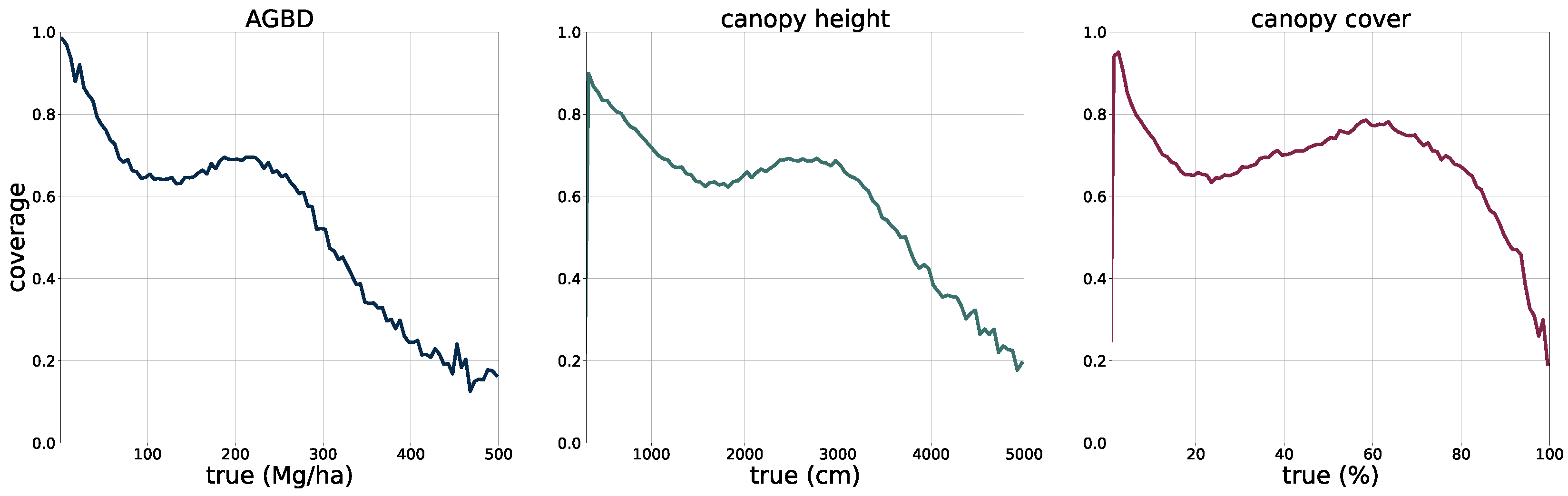
2.5. Model Performance Assessment

The deployment of the model on a global scale for the year 2023 allows for a qualitative assessment of its performance, in particular in challenging areas such as those with high cloud coverage, which may affect the quality of the input imagery.

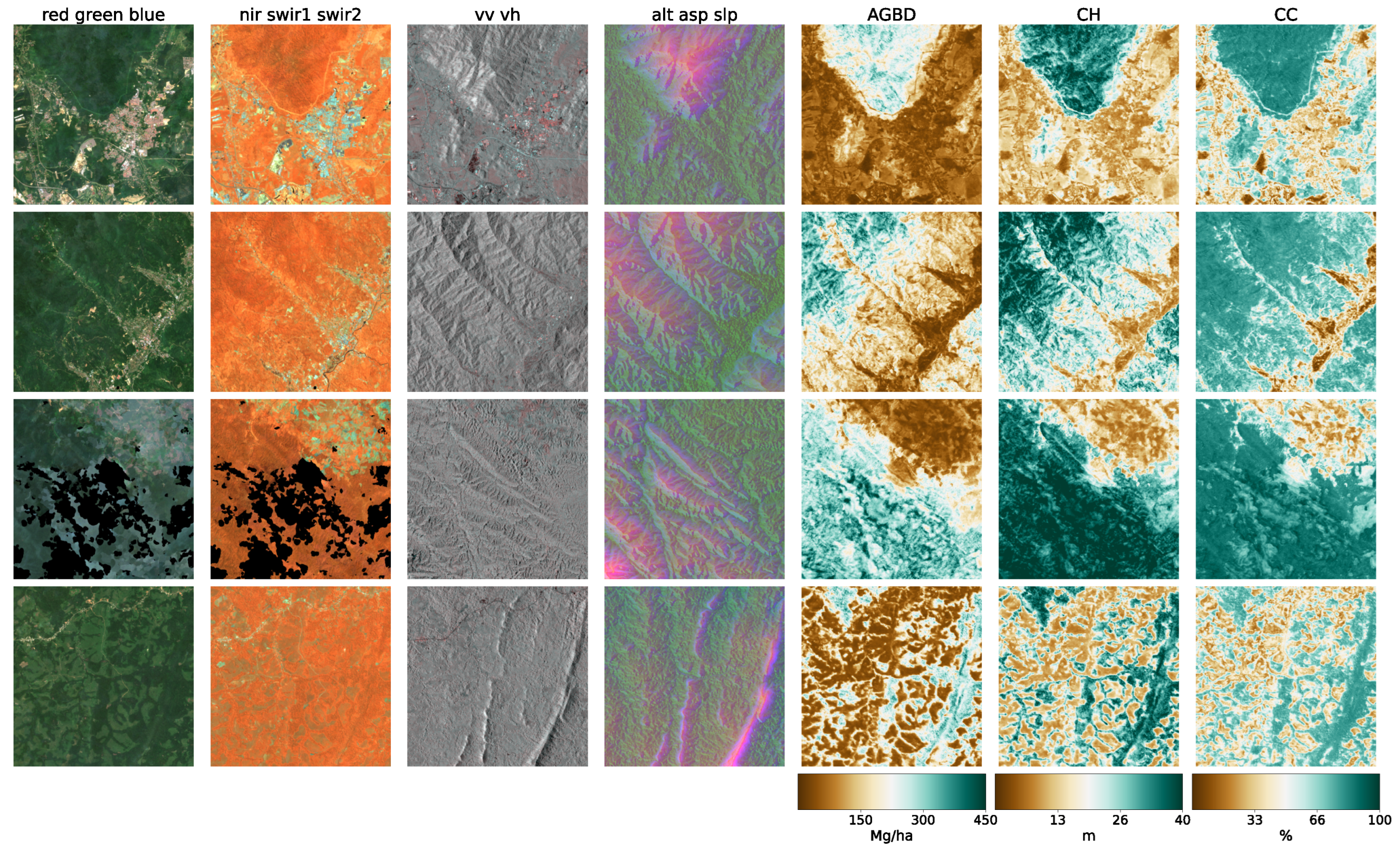
In Figure 5, we present four sample locations that cover an area of 1 km × 1 km at 10 m resolution. The four columns on the left represent the input data (excluding the geographic coordinates), while the three columns on the right correspond to the predictions of AGBD, CH, and CC. The top row represents a sample where the model performs very well. It contains various land-cover types such as urban, agriculture, and low- as well as high-density forest areas. The second row shows a sample in a high-density mountainous area with a nonforested valley. Both SAR backscatter and DEM provide valuable information on the terrain in this sample. The model performs as expected and successfully distinguishes high- from low-density and forested from nonforested areas. The third row demonstrates the model’s ability to leverage the multisensor input stack. There are multiple regions where the cloud-free composite left gaps visible as black areas in Sentinel-2 data. Here, information from Sentinel-1 and DEM is used to improve the predictability of these areas. The last row illustrates the model’s capability for making accurate predictions at high resolution. The example shows individual trees, or groups of trees, that are well separated from the bare ground.

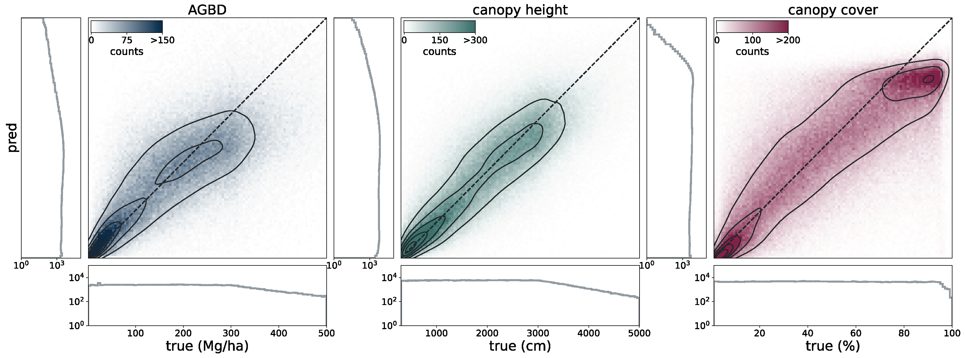
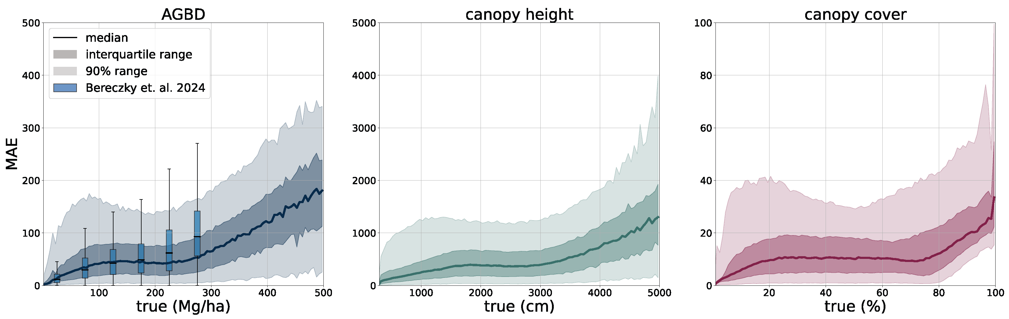
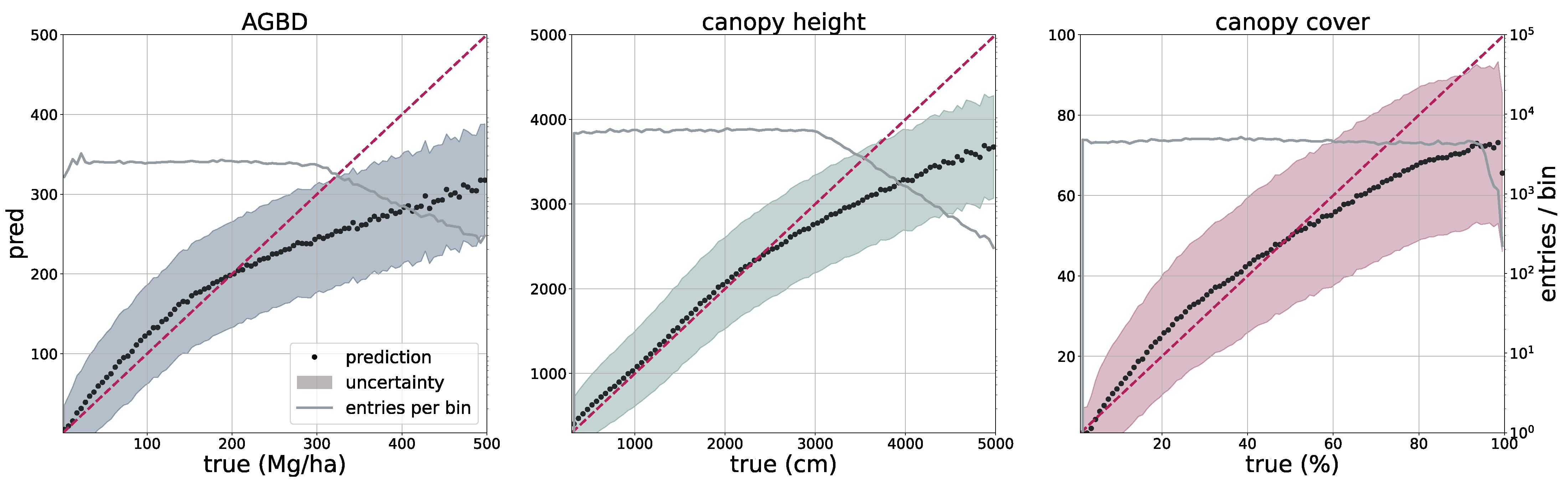
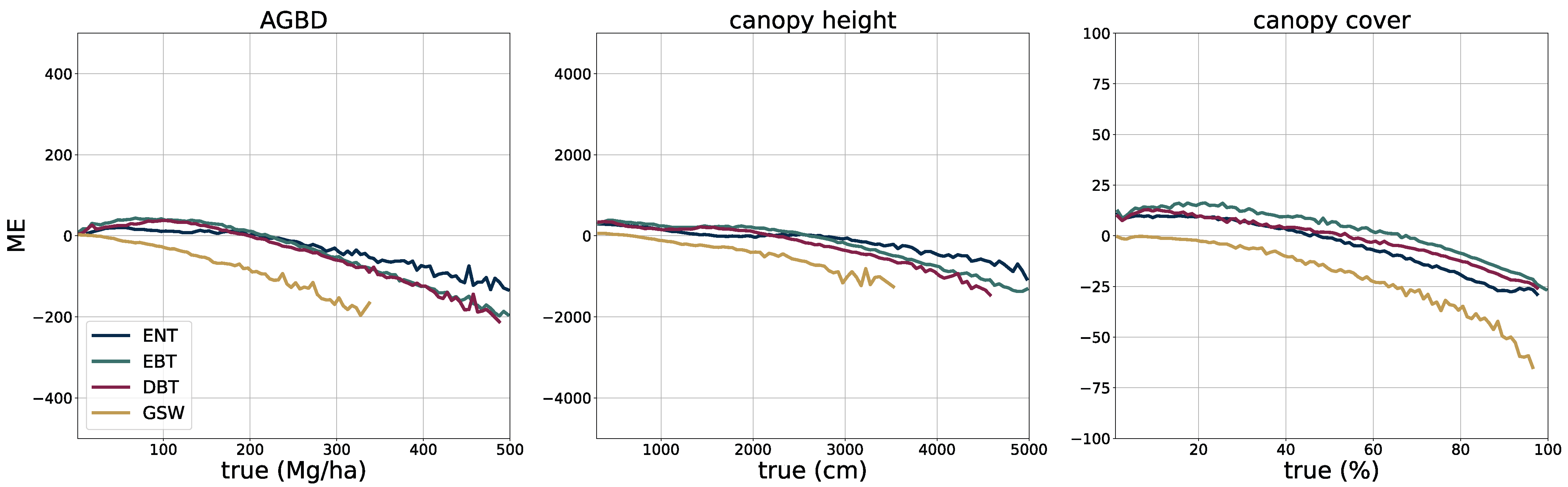
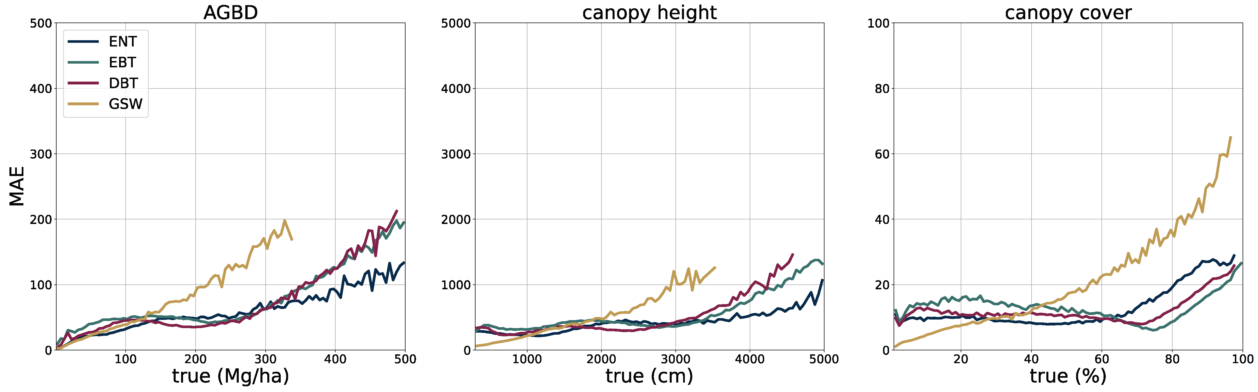
To validate the accuracy of the model, we use the held-out test set consisting of 14,745 samples and 13.8 M individual GEDI footprints. Model inference is performed on each test sample of size 256 pixels × 256 pixels, which generates predictions for every pixel and all output variables, including their uncertainties. We measure the correlation (corr), mean error (ME), mean absolute error (MAE), mean absolute percentage error (MAPE), and root mean squared error (RMSE), defined as

$$\mathrm{corr}={\displaystyle \frac{{\sum }_i(y_i-{\mu }_y)({\widehat{y}}_i-{\mu }_{\widehat{y}})}{\sqrt{{\sum }_i{(y_i-{\mu }_y)}^2{\sum }_i{({\widehat{y}}_i-{\mu }_{\widehat{y}})}^2}}}$$

(14)

$$\mathrm{ME}={\displaystyle \frac{1}{N}}\sum _{i=0}^N(y_i-{\widehat{y}}_i)$$

(15)

$$\mathrm{MAE}={\displaystyle \frac{1}{N}}\sum _{i=0}^N|y_i-{\widehat{y}}_i|$$

(16)

$$\mathrm{MAPE}={\displaystyle \frac{1}{N}}\sum _{i=0}^N{\displaystyle \frac{|y_i-{\widehat{y}}_i|}{{\widehat{y}}_i}}$$

(17)

$$\mathrm{RMSE}=\sqrt{{\displaystyle \frac{1}{N}}\sum _{i=0}^N{(y_i-{\widehat{y}}_i)}^2}$$

(18)

between the GEDI ground truth data ${\widehat{y}}_i$ and the model predictions $y_i$ gathered at the pixel coordinates of the GEDI footprints. Due to the non-uniform distribution of ground truth values, we assess the model performance on both the test set with its original and uniform sample distribution. For this purpose, we sample data points according to the inverse PDF of each variable’s respective distribution. This ensures a more fair performance assessment in the value ranges of each variable. Due to the low frequency of the appearance of high values of AGBD and CH, we set a reference value of 300 Mg/ha for AGBD and 30 m for CH to define the lowest probability value. Values with lower probabilities are always included during sampling. After the sampling procedure, a total number of 200 k–450 k data points remain, depending on the variable. We provide the detailed results of this evaluation in Section 3.1.

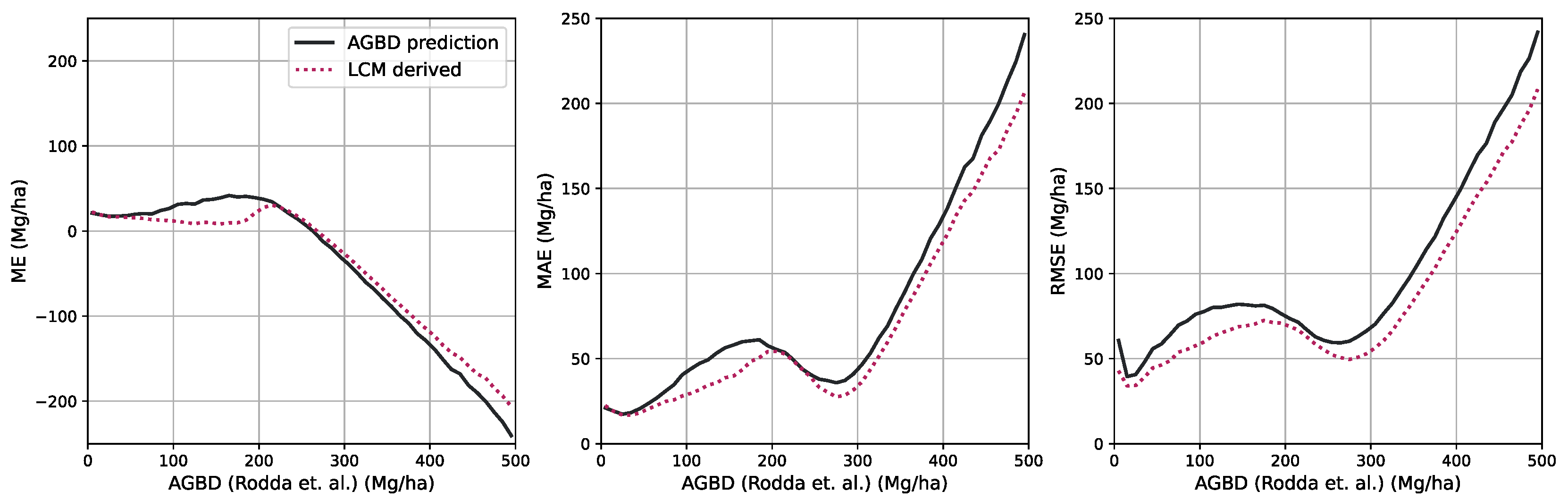
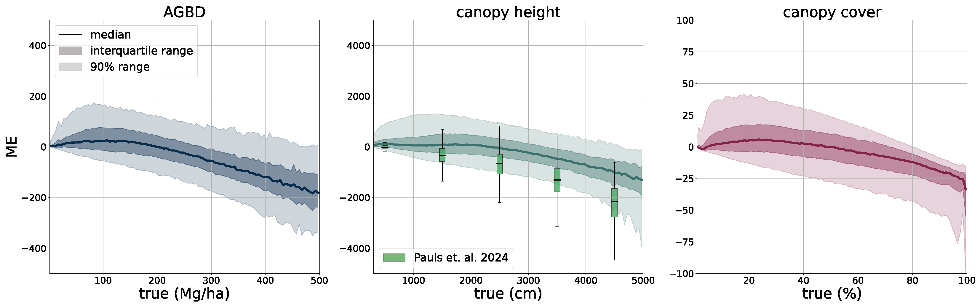
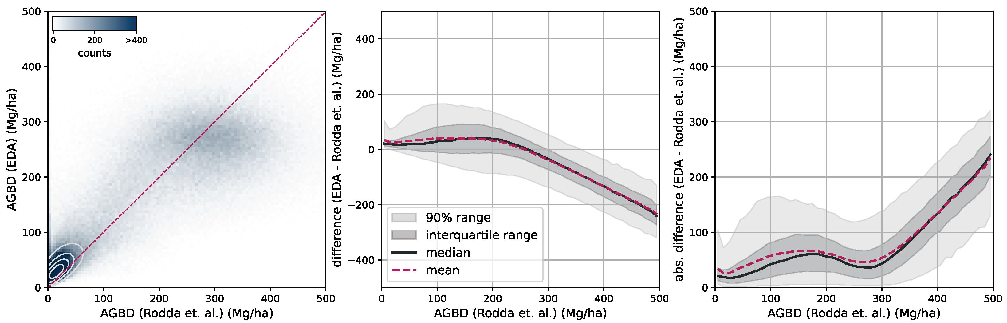
Using the test set for model evaluation is a fair way to assess the predictive skills of the model but assumes accurate ground truth labels. In order to account for systematic errors and further evaluate the model on independently collected ground measurements, we select two third-party datasets, one for ABGD and one for CH, to which we compare our model predictions.

Aboveground biomass. For the verification of biomass estimates, we utilize the dataset created by [58] which consists of 13 plots of variable size at a maximum resolution of 40 m. Eight of the plots are located in the Central African region, and five of the plots are in the South Asia region. This dataset was compiled from forest inventory collected at the respective sites during different time ranges. Site-level measurements followed a strict protocol in which the diameter at breast height (DBH) was determined for each individual tree within the plots, as well as the tree height (H) for a subset of trees. Tree-level taxonomic identification and relative coordinates within the plots were recorded along with geographic coordinates of the plot borders at intervals of 20 m. The forest inventories were split into 1 ha and 0.16 ha plots. The data collected for DBH-H on a subset of trees within these plots were used to fit allometric equations that relate H to DBH and allow the extrapolation of tree height measurements to all trees in the plots. Then the wood density based on the tree taxonomy was used to calculate the aboveground biomass reference (${\mathrm{AGB}}_{ref}$). Aerial LiDAR at a resolution of 1 m was obtained over the sites within an absolute temporal difference of 2.2 ± 1.9 years from the forest inventory dates. From the LiDAR data, canopy height models (CHM) and canopy metrics (LCM) were derived. Allometric equations of the form

$$log\left({\mathrm{AGB}}_{ref}\right)=a+b·log\left(\mathrm{LCM}\right)+{\mathrm{RE}}_{site}+ϵ$$

(19)

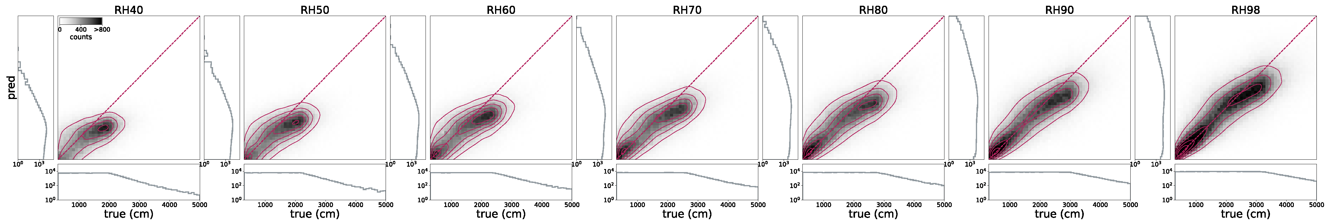
were then fit, which relates LCM to AGB. The authors found that the average of RH40, RH50, RH60, RH70, RH80, RH90, and RH98 represents the best predictor of LCM for AGB.

For this study, we utilize the 40 m resolution dataset since it is closer to the native resolution of our model. For the comparison, we resample our model output to 40 m resolution using the average resampling method. We deployed our model over all sites for the year the forest inventory ended at the respective site. Due to limitations of input data availability, our model can only be deployed back to the year 2017. For sites with forest inventory dates prior to 2017, we chose 2017 as the deployment year. 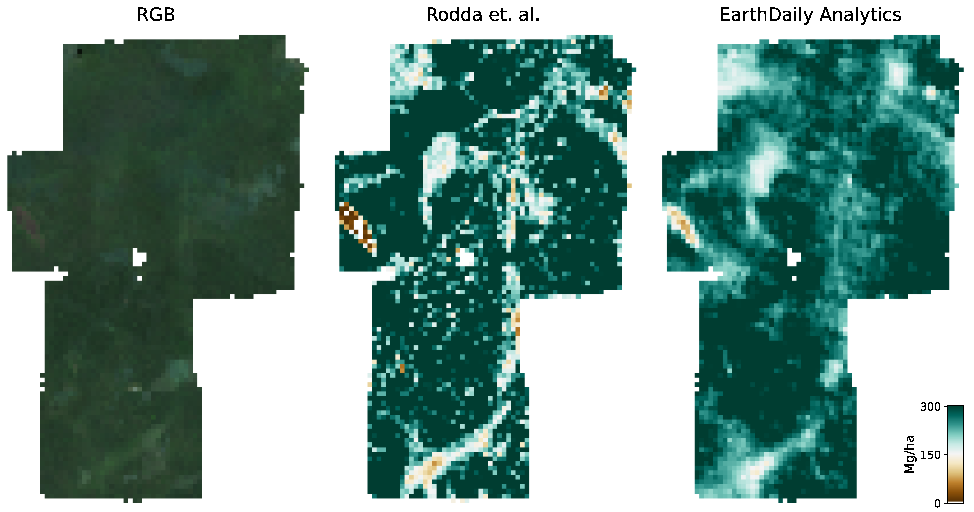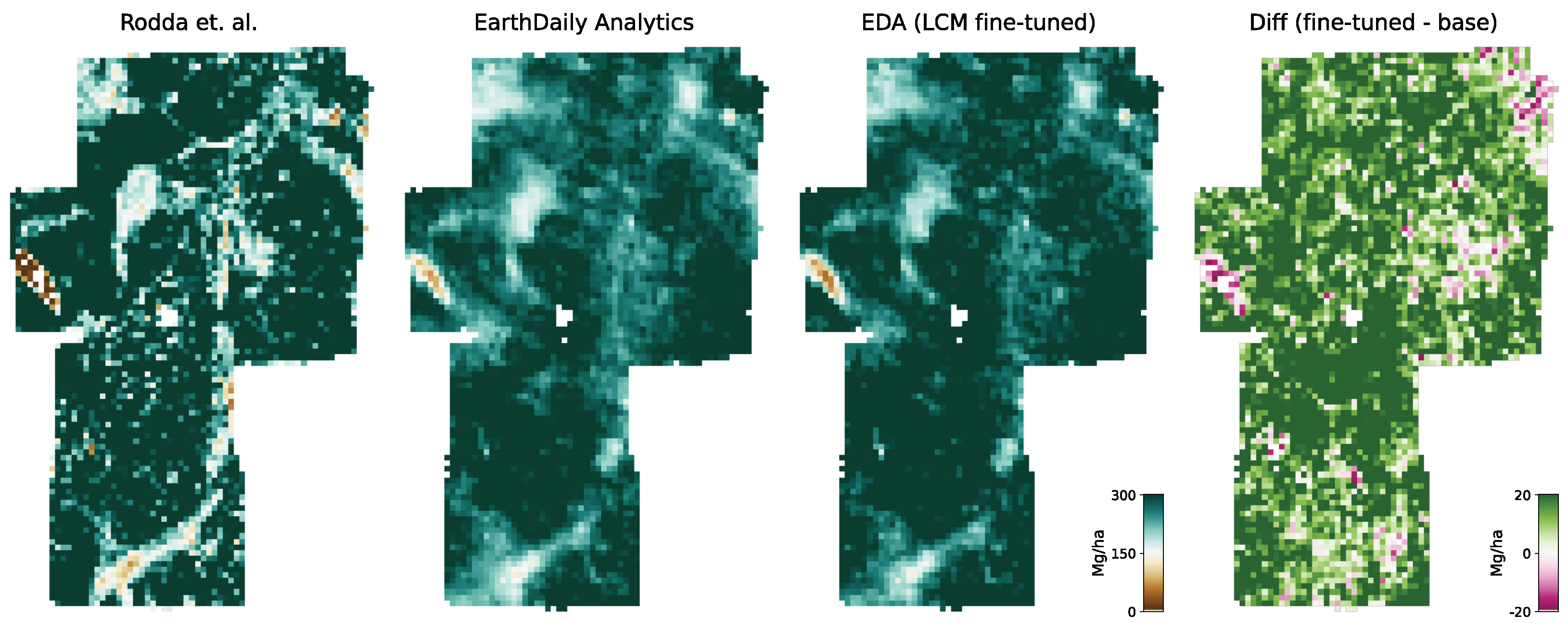Figure 6 shows an RGB image of the input data, the reference AGBD, as well as our model’s estimate for AGBD for the site Somaloma, Central Africa.

We consider each pixel of 40 m × 40 m size (0.16 ha) as a data point and compare the AGBD estimate by our model with the ground measurement provided by [58]. We determine RMSE, ME, and MAE across all pixels and sites except Achanakmar, Betul, and Yellapur, which we exclude from this study. For these three sites, we noticed that our model underestimates AGBD. Upon further investigation, we found the underestimation to be caused by the input compositing strategy. The three sites contain a large fraction of deciduous broadleaf trees and are located in the tropical region for which we construct cloud-free composites over a 6-month time period. In these particular cases, this resulted in the inclusion of scenes where the trees did not carry leaves, causing a shift in the input signal. This can be addressed by shortening the composite time window for regions with these conditions, which we reserve for future work.

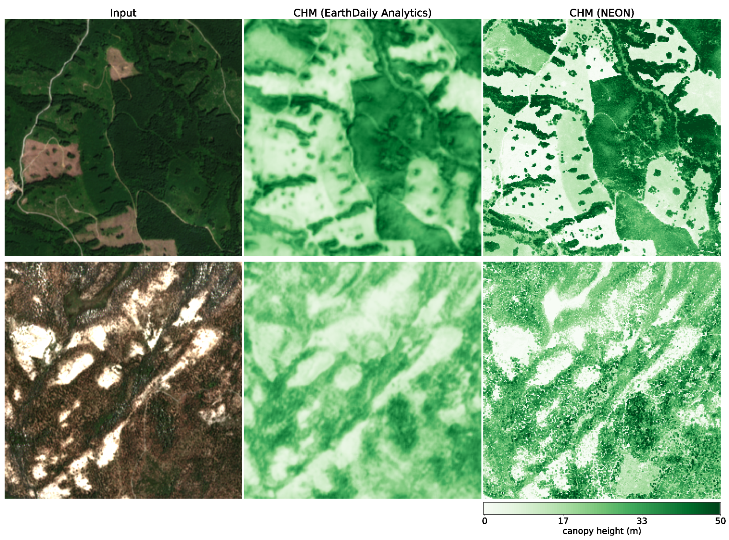
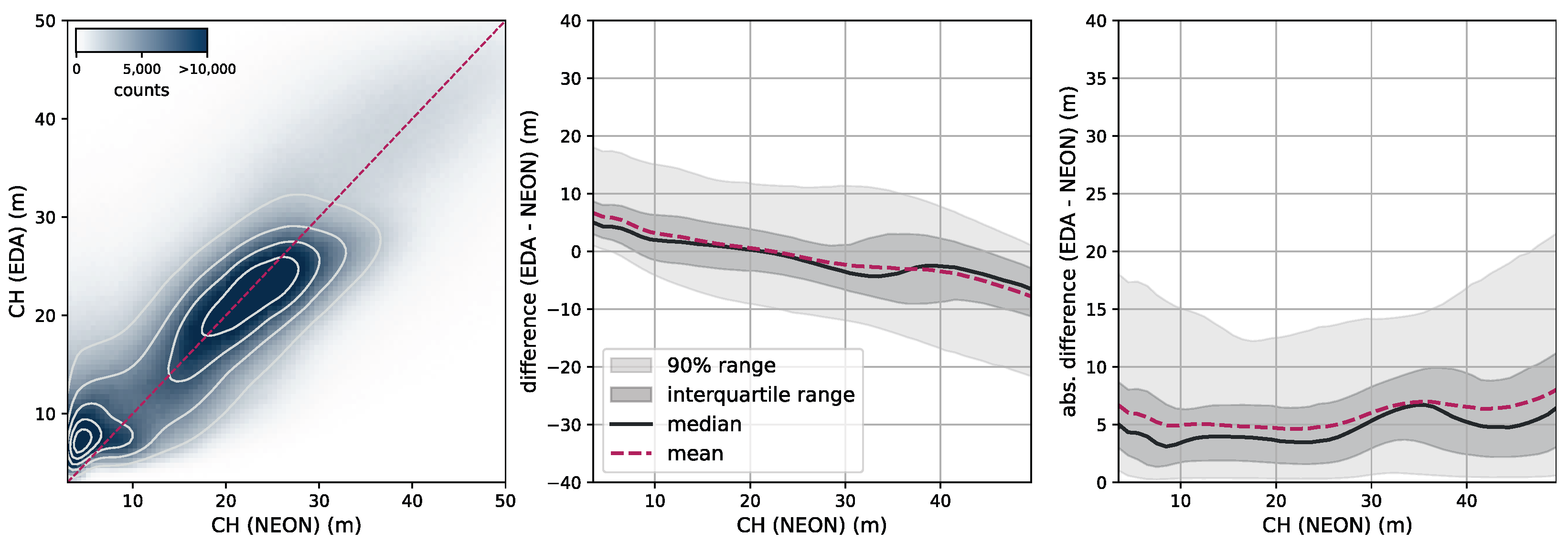
Canopy height. To further assess our model CH estimation, we use data from the National Ecological Observatory Network (NEON) [39]. NEON is a high-resolution LiDAR dataset that provides detailed three-dimensional information about the Earth’s surface. This dataset includes measurements of vegetation structure, topography, and land cover in diverse ecological regions in the United States. Data are collected using airborne LiDAR sensors, capturing fine-scale details at a resolution of 1 m. We selected all measurement sites in the states of AL, CA, FL, GA, OR, UT, VA, and WA from the year 2021. We subdivide each site into areas of size 2560 m × 2560 m and rasterize our model CH estimation as well as the NEON CH measurement at their respective resolutions (10 m for our model and 1 m for NEON). This results in tiles of size 256 pixels × 256 pixels (our model) and 2560 pixels × 2560 pixels (NEON). In order to compare the two maps, we resample the NEON map by determining the 98th percentile in each 10 pixels × 10 pixels area, resulting in a map of the same pixel size as our models. We chose this approach because our model effectively estimates the RH98 metric for each pixel corresponding to 10 pixels × 10 pixels in the NEON map. Figure 7 illustrates the RGB imagery and the CH maps of our model and NEON for two samples (the top row corresponds to a sample in site ABBY, WA, and the bottom row to a sample in site TEAK, CA).

3. Results

In this section, we discuss the results of evaluating our model by determining the metrics introduced in Section 2.5 on the test dataset. We also compare the model predictions against independent datasets that focus on the variables AGBD and CH.

3.1. Predictive Performance Results

Determining the evaluation metrics defined in Equations (14)–(18) on the held-out test set provides a measure of the predictive skills of the model. In

Table 1. Summary of evaluation metrics for all prediction variables and both the original test set and a subset created by uniform sampling across all variables. The units for AGBD (CH, CC) are Mg/ha (cm, %) except for correlation, which is unitless and MAPE, which is given in %.

	Uniform					Original
Variable	Corr	ME	MAE	MAPE	RMSE	Corr	ME	MAE	MAPE	RMSE
AGBD	0.70	−10.83	62.95	48.03	86.74	0.83	10.75	26.07	166.60	50.59
CH	0.80	−20.09	455.46	27.56	624.94	0.85	83.51	370.95	35.19	543.81
CC	0.75	−3.40	13.92	45.26	18.68	0.88	−1.92	9.86	104.10	15.75

we summarize all metrics for the variables AGBD, CH, and CC separately for both the uniformly sampled and original datasets.

These metrics are representative of the model performance across the full range of variable values. In order to get a better understanding of the model performance at various ground-truth values, we also create binned evaluation metrics. We aggregate the sample pairs ${\mathbf{y}}^i=(y_{\mathrm{true}}^i,y_{\mathrm{pred}}^i)$ for each variable $i\in 0,1,2$, where $y_{\mathrm{true}}^i$ falls within a specific bin and calculate the metrics for each bin separately. The bin range and bin size $(b_{\mathrm{low}},b_{\mathrm{high}},b_{\mathrm{size}})$ for AGBD are (0, 500, 5) Mg/ha, for CH (0, 5000, 50) cm, and for CC (0, 100, 1)%. Figure 8 shows a scatter plot of samples ${\mathbf{y}}^i$ for each variable i, where the color map represents the sample density. The distributions of $y_{\mathrm{true}}$ and $y_{\mathrm{pred}}$ are shown in the bottom and left panels. Overall, there is very good agreement between the predicted and true values in all variable ranges. However, there is an increased disagreement at higher values of AGBD and CH. This can be attributed to the lower amount of training samples in these regions as well as to signal saturation in the input data.

In Figure 9 and Figure 10, the median error (absolute error) within each bin (solid line) as well as the interquartile range, which contains 50% of all data points (dark shaded area), and the 90% range (lightly shaded area) are shown. The plots further illustrate the good agreement of the model predictions with ground truth data. For AGBD, we observe a slight overprediction within the range of 0–200 Mg/ha and a slight underprediction for values > 200 Mg/ha. The CH predictions agree very well up to values of 25 m, where the model starts to slightly underpredict. For CC, the agreement is very good across the range of values, except for full coverage (close to 100%), where the model tends to slightly underestimate. It should be noted that the evaluation metrics determined in the full variable range (as shown in Table 1) are biased towards larger values due to outliers that can have a large contribution when using a uniformly sampled dataset. On the other hand, the metrics may be biased towards smaller values when using the original sample distribution because lower values (and therefore smaller errors) are more frequent. This is an important consideration when comparing results across different works since the sample distributions and the ranges within which they are defined are different. In this work, we present all metric plots based on the uniformly sampled dataset, as this provides the least bias, and include the results on the original dataset in Table 1.

We compare our results with the most recent and state-of-the-art results of [8] for AGBD and [9] for CH. Their corresponding error metrics are included in Figure 10 (left) and Figure 9 (middle) as well as in

Table 2. Comparison of mean absolute AGBD estimation error per bin range of our model against the previous state-of-the-art method from [8]. The numbers in bold indicate best performance.

	Bin Range (Mg/ha)
Method	0–50	50–100	100–150	150–200	200–250	250–300
EarthDaily Analytics	12.6	34.2	45.0	44.2	43.7	54.7
Bereczky et al. [8]	11.55	29.62	42.63	48.76	61.93	93.13

and

Table 3. Comparison of mean CH estimation error per bin range of our model against previous state-of-the-art methods. Both [9] and [33] use a CNN-based model, while [7] uses a classical machine-learning approach with a random forest model. The numbers in bold indicate best performance.

	Bin Range (cm)
Method	0–1000	1000–2000	2000–3000	3000–4000	4000–5000
EarthDaily Analytics	88.5	70.5	−57.9	−398.5	−919.2
Pauls et al. [9]	−32.0	−352.0	−650.0	−1313.0	−2167.0
Lang et al. [33]	−366.0	−724.0	−635.0	−1144.0	−2241.0
Potapov et al. [7]	−331.0	−1081.0	−1357.0	−1851.0	−2841.0

. Our model performance on AGBD is comparable with [8] in the range of 0–200 Mg/ha but shows improved performance above 200 Mg/ha, which corresponds to regions where a large portion of the world’s biomass is stored, such as rain forests, and is therefore of great importance. For CH, our model outperforms [9] throughout the range except for small trees (<10 m), where both approaches show comparable results. We also include the results of [7,33] in our comparison, as summarized in Table 3. We did not find previous work on CC that fits the scope of this study for a one-to-one comparison. However, we conduct an analysis of deforestation detection in Section 4.2, where we compare our results with [41].

Finally, Figure 11 shows the median predictions within each bin as a function of the true values. The shaded areas correspond to the median standard error prediction of all samples within a given bin. These plots further demonstrate the good agreement of our model predictions with ground truth data in the low-to-mid variable range, while it tends to underestimate at high values of the prediction variables. The underestimation of AGBD and CH can be attributed to the lack of training data at very high values, as well as a saturation effect at the input level. For AGBD, there is an additional effect that arises from the increasing uncertainties of the ground truth at higher values of AGBD. We further discuss the implications of the prediction uncertainties in Appendix B.2. The 1$\sigma$ uncertainty bands are slightly overestimated at lower values for all variables since the coverage exceeds 68% and are slightly underestimated at higher values where the coverage is <68%. We reserve addressing this discrepancy for future work but provide the exact coverages in Appendix B.1.

The above model performance assessment is performed using samples from all regions of the world and plant functional types (PFT). To further assess the accuracy of the models with respect to the different PFTs, we repeat the analysis on samples grouped by PFT, where we retrieve the PFT class from the GEDI dataset and categorize them as Deciduous Broadleaf Trees (DBT), Evergreen Broadleaf Trees (EBT), Evergreen Needleleaf Trees (ENT), and Grasslands/Shrublands/Woodlands (GSW).

Table 4. RMSE for all variables based on plant functional types (PFT). The units for AGBD (CH, CC) are Mg/ha (cm, %).

Variable	DBT	EBT	ENT	GSW
AGBD	66.98	84.33	66.53	24.30
CH	585.31	700.01	608.94	318.72
CC	21.82	21.53	21.19	9.05

summarizes the RMSE values determined for all variables and PFT. Figure 12 and Figure 13 show the median error and the median absolute error for each bin, separated by the different PFTs. For these plots, we only include bins with >50 entries/bin.

In general, the model performs best on samples of class ENT, followed by DBT and EBT, as measured by the RMSE metric on the full variable scales for AGBD and CH, while for CC it shows comparable performance across the classes. We exclude GSW from this ranking, even though it shows the lowest RMSE because most samples in this class cluster at low values. This distribution skews the RMSE downward, as the metric reflects absolute differences and tends to produce lower values when the true values themselves are small. The opposite effect is true for the EBT class, where many of the samples cluster at high values and, therefore, contribute to higher RMSE. In addition, the saturated input signals at high values of AGBD and the limitations to height estimation due to resolution further increase the errors. The classes ENT and DBT both have a more uniform sample distribution, causing the model performance to be less affected by the saturation effects and the RMSE metric to be skewed.

3.2. Assessment Against Third-Party Datasets

In the following section, we present the results from studies where we compared our model’s output with third-party datasets that are independent of the GEDI measurements. All these datasets were generated from high-resolution airborne LiDAR or on-the-ground measurements. We deployed our model over the respective regions for the years the ground-truth data were collected. We divide our studies into estimation of aboveground biomass and canopy height since the datasets are focused on one of these variables. Section 2.5 provides more details on the data and methods used for each study.

3.2.1. Aboveground Biomass

As introduced in Section 2.5, we use the dataset of [58] in this study. Figure 14 summarizes the results of this study. The figure on the left shows a 2D histogram of our model estimate vs. the ground measurement for each pixel. There is a clear correlation, and we measure an R² value of 0.39. The figure in the middle (right) shows the median error (median absolute error) for each bin of size 5 Mg/ha as well as the range of the interquartile (dark-shaded area) and 90% (lightly shaded area) range.

These plots show the same pattern as the validation results against the GEDI test dataset (Figure 9 and Figure 10), where the error is generally small in the range of 0–300 Mg/ha and increases in the region >300 Mg/ha. This illustrates that there may be limitations related to both the input signal, due to saturation effects, as well as the training data, which exhibit increasing uncertainties with larger values of AGBD. The authors of this dataset specifically mention the importance of such ground measurements for recalibration purposes since the accuracy of AGBD estimates from large-scale LiDAR surveys (such as GEDI) is often limited due to the availability of calibration data. In this study, we report the results of testing our model estimates without recalibration, which we plan to do in future work. In general, we measure an ME of −6.46 Mg/ha, an MAE of 60.21 Mg/ha, and an RMSE of 84.95 Mg/ha. We also determined the total amount of biomass in all sites considered for this study to be 8.62 Mt based on our model estimate, while the total amount based on [58] is 8.95 Mt, corresponding to a 3.63% difference.

3.2.2. Canopy Height

The visual comparison between our model CH estimation and NEON CH measurement based on the sample locations provided in Figure 7 shows very good agreement despite the fact that our model’s CH map is at 10× lower resolution. We quantify the agreement between our and NEON’s CH map by calculating RMSE, ME, and MAE, considering all pixel values from all tiles and sites as data points. Overall, we achieve an RMSE of 7.46 m, an ME of 0.17 m, and an MAE of 5.57 m. Figure 15 shows a 2D histogram of all data points, as well as ME and MAE, aggregated in bins of size 1 m with respect to the NEON CH. The R² value of the model predictions compared with the NEON measurements is 0.51. We also illustrate the error distribution within each bin by indicating the interquartile as well as the 90% range. The red dashed line corresponds to the mean in each bin.

The agreement between our and NEON’s CH map is very good across the entire value range. We note that there is some larger disagreement at low values (<5 m), which is also visible in the sample maps in Figure 7, where our model generally estimates slightly higher values at small CH. This can be attributed to the fact that the GEDI dataset contains a very small number of data points < 3 m, so the model generally overestimates in this region. However, it is notable that the absolute error mostly stays below 5 m across the entire value range up to 50 m. The NEON dataset offers the capability to recalibrate the model estimations where it exhibits a bias. This is true for any high-accuracy regional dataset. We reserve the demonstration of recalibration of the model for future work.

4. Applications

In this section we demonstrate some use cases of our model, including the monitoring of changes over time as well as fine-tuning the model on regional ground truth data to better align the global model to local conditions. Traditionally, many use cases require the deployment of multiple models in order to perform a downstream task, where each model output provides the solution for subtasks. One of the main motivations of this work is to create a single model that is versatile enough to provide results for all subtasks in one forward pass. One such application is the detection of deforestation and association of loss of biomass, which we discuss in detail in Section 4.2.

4.1. Global Model Deployment

Our model is scalable both spatially and temporally due to its global training dataset. This is an important factor when it comes to monitoring changes in ecosystems. Although global deployments may not be required very frequently, deployments over local regions of interest can be performed rapidly at temporal resolutions of <1 year. We generated global maps for all three prediction variables AGBD, CH, and CC, as well as their uncertainties at 10 m resolution for recent years. They cover the latitude range of 57°S to 67°N according to the availability of Sentinel-1 data. The deployment year is 2023 for all regions except for the areas where Sentinel-1 experienced an outage for that year. In this case, we filled the gaps with the most recent available observations, which in most cases is 2021. The deployment was performed in two steps using scalable batch compute from AWS: First, we generate cloud-free composites, pulling data from the Descartes Labs platform, for global image tiles of size 1024 pixels × 1024 pixels. The tiles were generated using the Descartes Labs tiling system. We follow the same schema for determining the composite time window as for the training dataset (see Section 2.2.2). The image composites are saved as a product in the Descartes Labs platform for fast retrieval during inference. In the second step, we perform model inference on tiles of size 2048 pixels × 2048 pixels with a padding of 80 pixels. The output of the deployment is stored as a product in the Descartes Labs platform and consists of multiple layers representing the prediction variables, as well as multiple mask layers. The mask layers are either forward propagated from the composite product, such as a composite gap mask, or derived from the model output, such as a forest mask. Figure 16 (as well as Figure 1) shows the low-resolution maps for all prediction variables.

4.2. Monitoring Biomass Change and Deforestation Detection

The monitoring of global deforestation and carbon accounting has become an important part of climate change mitigation, where remotely sensed data plays an integral part in many models developed in the past. Most of these models utilize optical or SAR-based imagery and are based on a variety of approaches, from pixel-based anomaly detection in time series data [59] to modern deep learning and computer vision algorithms [60]. In this section, we demonstrate the usability of our model for the task of deforestation detection and accounting for corresponding loss in biomass. We selected an area in Brazil at location 59°26′46″W, 7°1′4″S with a total area of 507 kha.

We deployed our model in the area for each year from 2017 to 2023. Figure 17 shows the AGBD map for 2017 (left) and 2023 (middle), respectively. In this study, we measure changes year by year and compare the results with Global Forest Watch [41], which provides annual tree cover loss data based on observations from Landsat at 30 m resolution. We follow their approach to define forested land by requiring CH > 5 m and determine the regions with significant canopy cover loss (∆CC > 20%). Figure 17 (right) shows the regions that meet these requirements accumulated between 2017 and 2023. Note that not all regions correspond to complete deforestation but rather significant loss of tree cover, according to the definition by Global Forest Watch. We aggregated areas with tree cover loss for each year, with respect to the previous year, and compared our numbers to those reported by Global Forest Watch. Figure 18 summarizes the results. Our numbers agree with those of Global Forest Watch to within 10% on average. We determine the total area of tree cover loss during the 6-year time span to be 103.3 kha, while Global Forest Watch reports a number of 101.2 kha, a difference of 2.1%. In addition to the total area of tree cover loss, our model also provides the amount of biomass lost in these areas by taking the difference between AGBD maps in 2017 and 2023 and multiplying it by the total area. We measure a total loss in biomass of 14.9 Mt, equivalent to 25.66 Mt of CO₂.

This study highlights the practicality of our model as a unified approach for simultaneous prediction of multiple relevant variables, and it makes it easily scalable to other regions in the world.

4.3. Model Fine-Tuning for Local Conditions

One of the main contributors to the uncertainty of AGBD estimations is the limited availability of ground measurements to calibrate allometric equations at a global scale. However, estimations of canopy height metrics do not depend on such calibrations, as they are derived from the LiDAR waveforms directly. Our model, therefore, offers a unique capability for fine-tuning local conditions in order to achieve more accurate AGBD estimations. The majority of allometric equations use relative height (RH) metrics as predictors for AGBD, which our model is able to estimate. The base model predicts AGBD, RH98, and CC. However, due to its multihead architecture, it can easily be fine-tuned on other variables. We demonstrate such a use case based on the data and coefficients for allometric equations provided by [58]. The authors determine the coefficients of the allometric equation in (19) for each of the 13 sites. They find that the average of all the RH metrics listed is the best predictor of AGBD. We expand our model to 7 heads, each representing one of the RH metrics, and fine-tune the weights of these heads for one epoch while keeping the weights of the encoder and decoder frozen. We apply sample weighting according to the inverse PDF of each variable’s distribution (see Appendix A for details). Figure 19 shows 2D histograms of the model estimates for each variable versus the true value, evaluated on a uniformly sampled test dataset.

Generally, there is very good agreement between the model predictions and the true values for all RH metrics. Detailed evaluation metrics are summarized in

Table 5. Summary of evaluation metrics for all RH variables from the fine-tuned model. All metrics are given in unit cm except corr which is unitless.

Metric	RH40	RH50	RH60	RH70	RH80	RH90	RH98
ME	−327.48	−283.10	−235.92	−185.50	−152.69	−112.22	−91.73
MAE	511.92	506.91	497.92	490.29	484.57	478.49	473.47
RMSE	653.74	657.18	654.83	652.30	648.12	647.48	642.94
corr	0.559	0.608	0.657	0.698	0.736	0.768	0.800

. We deployed the fine-tuned model over the sites given by [58] using the same input data as in Section 3.2.1 and determined AGBD based on the site-specific allometric equations and the RH predictions of our model. Figure 20 shows AGBD maps for the Somalomo site, Central Africa, based on [58] (left), AGBD estimate from our base model (mid-left), AGBD derivation from the RH variables of our fine-tuned model (mid-right), and the difference between the fine-tuned and the base model (right). Visually, there are subtle differences between our base and fine-tuned models. However, the fine-tuned model decreases the MAE by 15.3% to 50.96 Mg/ha and the RMSE by 16.2% to 71.18 Mg/ha. The R² value increases from 0.39 to 0.58.

For more details on the comparison between the base and fine-tuned models, see Appendix B.3. These results highlight the benefit of local model fine-tuning in order to incorporate regional calibrations of allometric equations, which our model is inherently designed for.

5. Discussion

Despite the need for global-scale monitoring of forest carbon pools, many technical challenges have limited the scalability and accuracy of solutions. In this work, we hypothesized that by leveraging (1) globally distributed source of ground truth, (2) fusion of multiple input sources, including non-optical imagery, and (3) training a single model on multiple correlated targets, we can achieve scale and address obstacles related to model performance, particularly in areas of large noise (e.g., due to cloud obstructions).

The model evaluation against individual, globally distributed GEDI measurements contained in the test dataset shows good agreement between the predictions and ground truth values as measured by various metrics. Compared with previous work that predicts AGBD [8] and CH [7,9,33] we achieve the lowest error across all ranges of variables on a global scale. This demonstrates the potential for novel model architectures and multi-modal data sources to address challenges in forest monitoring. In order to demonstrate the practicality of our model, it is important to validate its predictions against data samples which were collected with high precision and/or on the ground offering an independent data source. The model shows reasonable agreement with these third-party datasets across a wide range of ABGD and CH values. Because local measurements involve extensive human labor and are not readily available at scale in the public domain, this approach is used to generate consistent, global-scale estimates of forest carbon, which can fill gaps where local solutions are not available, serve as a tip-and-cue mechanism to prioritize ground studies, and facilitate comparative studies where consistent methodology is required.

The extensive model evaluation framework has shown that the predictions of all variables are of high accuracy at global scale, but exhibit limitations in very dense forests where input features are less distinct. This phenomenon has been well documented in the literature [61] and is caused by a limited spatial resolution and a saturation effect on the spectral sensitivity. This is an inherent limitation when using remotely sensed data as the information content is restricted. The effect is more severe with AGBD, which has an additional component from the increasing uncertainty of ground-truth samples at higher values due to the errors propagated from the calibration. Without additional data sources, such as high-resolution optical or SAR, it is difficult to overcome these limitations. At the same time, there is a trade-off between using high-resolution imagery and being able to update prediction maps frequently at low computational costs. With new satellite constellations being deployed in the near future, the methodology presented in this study holds great potential to further advance precision estimation from remote sensing data.

In addition to enhanced input data, our methodology will also benefit from more accurate ground-truth labels. The GEDI point data have an inherent uncertainty due to the relatively large footprint which manifests itself as noise in the training data. Machine learning models are generally able to deal with noisy data [62] at the cost of prediction accuracy. We observe this effect in our model predictions at higher values of AGBD and CH where the uncertainty of the ground-truth labels is higher, leading to underestimated predictions. Allowing the model to estimate the uncertainty through additional prediction heads provides a way to account for this limitation. As illustrated in Figure 11 and discussed in Appendix B.1, the model slightly overestimates the uncertainty band at low values and underestimates it at higher values, which is subject to future work and model improvements.

6. Conclusions

In this work we present a novel deep learning-based computer vision model that unifies the prediction of several biophysical indicators that describe the structure and function of vegetation in multiple ecosystems and their respective uncertainties. The model input consists of multiple satellite image sources including Sentinel-1 backscatter, multispectral Sentinel-2, and topographic information from SRTM. Previous studies have focused on the estimation of single variables with similar methodologies. Uncertainty estimations were also unavailable or conducted in separate studies. Training a single model for the prediction of AGBD, CH, and CC with a shared encoder-decoder architecture provides richer information for the extraction of common features. Additional benefits include efficient and cost-effective model deployment at scale, which are important factors for global monitoring efforts.

Our end-to-end training procedure using a weakly supervised learning method on point data representing individual measurements of the respective variables results in a skillful model as rigorously evaluated on a held-out test dataset achieving an RMSE of 50.59 Mg/ha (543.81 cm, 15.75%) for AGBD (CH, CC). We further evaluated our model against third-party datasets without further fine-tuning and attained performance that is consistent with or exceeds the expectations for such data, demonstrating the robustness and generalizability of our approach. In addition, we generated global maps of AGBD, CH and CC at 10 m resolution, extending the coverage of GEDI observations to a latitude range of 57°S to 67°N, for the year 2023 or 2021, respectively, where Sentinel-1 data were unavailable. This demonstrates the scalability of our model, due to its global training dataset.

References

1. FAO. Global Forest Resources Assessment 2020: Main Report; FAO: Rome, Italy, 2020. [Google Scholar]
2. IPCC. Climate Change 2021—The Physical Science Basis: Working Group I Contribution to the Sixth Assessment Report of the Intergovernmental Panel on Climate Change; Cambridge University Press: Cambridge, UK, 2023. [Google Scholar]
3. UNFCCC. The Paris Agreement. 2015. Available online: https://unfccc.int/process-and-meetings/the-paris-agreement (accessed on 19 August 2024).
4. Balestra, M.; Marselis, S.; Sankey, T.T.; Cabo, C.; Liang, X.; Mokroš, M.; Peng, X.; Singh, A.; Stereńczak, K.; Vega, C.; et al. LiDAR Data Fusion to Improve Forest Attribute Estimates: A Review. Curr. For. Rep. 2024, 10, 281–297. [Google Scholar] [CrossRef]
5. Dubayah, R.; Blair, J.B.; Goetz, S.; Fatoyinbo, L.; Hansen, M.; Healey, S.; Hofton, M.; Hurtt, G.; Kellner, J.; Luthcke, S.; et al. The Global Ecosystem Dynamics Investigation: High-resolution laser ranging of the Earth’s forests and topography. Sci. Remote Sens. 2020, 1, 100002. [Google Scholar] [CrossRef]
6. Kacic, P.; Thonfeld, F.; Gessner, U.; Kuenzer, C. Forest Structure Characterization in Germany: Novel Products and Analysis Based on GEDI, Sentinel-1 and Sentinel-2 Data. Remote Sens. 2023, 15, 1969. [Google Scholar] [CrossRef]
7. Potapov, P.; Li, X.; Hernandez-Serna, A.; Tyukavina, A.; Hansen, M.C.; Kommareddy, A.; Pickens, A.; Turubanova, S.; Tang, H.; Silva, C.E.; et al. Mapping global forest canopy height through integration of GEDI and Landsat data. Remote Sens. Environ. 2021, 253, 112165. [Google Scholar] [CrossRef]
8. Bereczky, M.; Chow, K.H.; Rashkovetsky, D.; Gottfriedsen, J. Global Aboveground Biomass Density Estimation from Sentinel-2 Imagery. In Proceedings of the ICLR 2024 Machine Learning for Remote Sensing (ML4RS) Workshop, Vienna, Austria, 11 May 2024; OroraTech GmbH: Munich, Germany, 2024. [Google Scholar]
9. Pauls, J.; Zimmer, M.; Kelly, U.M.; Schwartz, M.; Saatchi, S.; Ciais, P.; Pokutta, S.; Brandt, M.; Gieseke, F. Estimating Canopy Height at Scale. arXiv 2024, arXiv:2406.01076. [Google Scholar]
10. Pan, S.J.; Yang, Q. A Survey on Transfer Learning. IEEE Trans. Knowl. Data Eng. 2010, 22, 1345–1359. [Google Scholar] [CrossRef]
11. Penatti, O.A.B.; Nogueira, K.; dos Santos, J.A. Do deep features generalize from everyday objects to remote sensing and aerial scenes domains? In Proceedings of the 2015 IEEE Conference on Computer Vision and Pattern Recognition Workshops (CVPRW), Boston, MA, USA, 1–12 June 2015; pp. 44–51. [Google Scholar] [CrossRef]
12. Muszynski, M.; Klein, L.; da Silva, A.F.; Atluri, A.P.; Gomes, C.; Szwarcman, D.; Singh, G.; Gu, K.; Zortea, M.; Simumba, N.; et al. Fine-tuning of Geospatial Foundation Models for Aboveground Biomass Estimation. arXiv 2024, arXiv:2406.19888, 19888. [Google Scholar]
13. European Commission. Definitions and Obligations-Deforestation Regulation Implementation. 2024. Available online: https://environment.ec.europa.eu/topics/forests/deforestation/regulation-deforestation-free-products_en (accessed on 14 August 2024).
14. Wulder, M.A.; Masek, J.G.; Cohen, W.B.; Loveland, T.R.; Woodcock, C.E. Opening the archive: How free data has enabled the science and monitoring promise of Landsat. Remote Sens. Environ. 2012, 122, 2–10. [Google Scholar] [CrossRef]
15. Drusch, M.; Del Bello, U.; Carlier, S.; Colin, O.; Fernandez, V.; Gascon, F.; Hoersch, B.; Isola, C.; Laberinti, P.; Martimort, P.; et al. Sentinel-2: ESA’s Optical High-Resolution Mission for GMES Operational Services. Remote Sens. Environ. 2012, 120, 25–36. [Google Scholar] [CrossRef]
16. Donlon, C.; Berruti, B.; Buongiorno, A.; Ferreira, M.H.; Féménias, P.; Frerick, J.; Goryl, P.; Klein, U.; Laur, H.; Mavrocordatos, C.; et al. The Global Monitoring for Environment and Security (GMES) Sentinel-3 mission. Remote Sens. Environ. 2012, 120, 37–57. [Google Scholar] [CrossRef]
17. Veefkind, J.; Aben, I.; McMullan, K.; Förster, H.; de Vries, J.; Otter, G.; Claas, J.; Eskes, H.; de Haan, J.; Kleipool, Q.; et al. TROPOMI on the ESA Sentinel-5 Precursor: A GMES mission for global observations of the atmospheric composition for climate, air quality and ozone layer applications. Remote Sens. Environ. 2012, 120, 70–83. [Google Scholar] [CrossRef]
18. Irons, J.R.; Dwyer, J.L.; Barsi, J.A. The next Landsat satellite: The Landsat Data Continuity Mission. Remote Sens. Environ. 2012, 122, 11–21. [Google Scholar] [CrossRef]
19. Torres, R.; Snoeij, P.; Geudtner, D.; Bibby, D.; Davidson, M.; Attema, E.; Potin, P.; Rommen, B.; Floury, N.; Brown, M.; et al. GMES Sentinel-1 mission. Remote Sens. Environ. 2012, 120, 9–24. [Google Scholar] [CrossRef]
20. Markus, T.; Neumann, T.; Martino, A.; Abdalati, W.; Brunt, K.; Csatho, B.; Farrell, S.; Fricker, H.; Gardner, A.; Harding, D.; et al. The Ice, Cloud, and land Elevation Satellite-2 (ICESat-2): Science requirements, concept, and implementation. Remote Sens. Environ. 2017, 190, 260–273. [Google Scholar] [CrossRef]
21. Le Toan, T.; Quegan, S.; Davidson, M.; Balzter, H.; Paillou, P.; Papathanassiou, K.; Plummer, S.; Rocca, F.; Saatchi, S.; Shugart, H.; et al. The BIOMASS mission: Mapping global forest biomass to better understand the terrestrial carbon cycle. Remote Sens. Environ. 2011, 115, 2850–2860. [Google Scholar] [CrossRef]
22. Das, A.; Kumar, R.; Rosen, P. Nisar Mission Overview and Updates on ISRO Science Plan. In Proceedings of the 2021 IEEE International India Geoscience and Remote Sensing Symposium (InGARSS), Ahmedabad, India, 6–10 December 2021; pp. 269–272. [Google Scholar] [CrossRef]
23. Paheding, S.; Saleem, A.; Siddiqui, M.F.H.; Rawashdeh, N.; Essa, A.; Reyes, A.A. Advancing horizons in remote sensing: A comprehensive survey of deep learning models and applications in image classification and beyond. Neural Comput. Appl. 2024, 36, 16727–16767. [Google Scholar] [CrossRef]
24. Zhang, Y.; Liang, S.; Yang, L. A Review of Regional and Global Gridded Forest Biomass Datasets. Remote Sens. 2019, 11, 2744. [Google Scholar] [CrossRef]
25. Saatchi, S.; Harris, N.; Brown, S.; Lefsky, M.; Mitchard, E.; Salas, W.; Zutta, B.; Buermann, W.; Lewis, S.; Hagen, S.; et al. Benchmark map of forest carbon stocks in tropical regions across three continents. Proc. Natl. Acad. Sci. USA 2011, 108, 9899–9904. [Google Scholar] [CrossRef]
26. Baccini, A.; Goetz, S.J.; Walker, W.S.; Laporte, N.T.; Sun, M.; Sulla-Menashe, D.; Hackler, J.; Beck, P.S.A.; Dubayah, R.; Friedl, M.A.; et al. Estimated carbon dioxide emissions from tropical deforestation improved by carbon-density maps. Nat. Clim. Change 2012, 2, 182–185. [Google Scholar] [CrossRef]
27. Baccini, A.; Walker, W.; Farina, M.; Houghton, R.A. CMS: Estimated Deforested Area Biomass, Tropical America, Africa, and Asia, 2000; ORNL DAAC: Oak Ridge, TN, USA, 2016. [Google Scholar]
28. Hu, T.; Su, Y.; Xue, B.L.; Liu, J.; Zhao, X.; Fang, J.; Guo, Q. Mapping global forest aboveground biomass with spaceborne LiDAR, optical imagery, and forest inventory data. Remote Sens. 2016, 8, 565. [Google Scholar]
29. Yang, L.; Liang, S.; Zhang, Y. A New Method for Generating a Global Forest Aboveground Biomass Map From Multiple High-Level Satellite Products and Ancillary Information. IEEE J. Sel. Top. Appl. Earth Obs. Remote Sens. 2020, 13, 2587–2597. [Google Scholar] [CrossRef]
30. Dubayah, R.O.; Armston, J.; Healey, S.P.; Yang, Z.; Patterson, P.L.; Saarela, S.; Stahl, G.; Duncanson, L.; Kellner, J.R. GEDI L4B Gridded Aboveground Biomass Density, Version 2; ORNL DAAC: Oak Ridge, TN, USA, 2022. [Google Scholar]
31. Sialelli, G.; Peters, T.; Wegner, J.D.; Schindler, K. AGBD: A Global-scale Biomass Dataset. arXiv 2024, arXiv:2406.04928. [Google Scholar]
32. Li, W.; Niu, Z.; Shang, R.; Qin, Y.; Wang, L.; Chen, H. High-resolution mapping of forest canopy height using machine learning by coupling ICESat-2 LiDAR with Sentinel-1, Sentinel-2 and Landsat-8 data. Int. J. Appl. Earth Obs. Geoinf. 2020, 92, 102163. [Google Scholar] [CrossRef]
33. Lang, N.; Jetz, W.; Schindler, K.; Wegner, J.D. A high-resolution canopy height model of the Earth. Nat. Ecol. Evol. 2023, 7, 1778–1789. [Google Scholar] [CrossRef] [PubMed]
34. Oquab, M.; Darcet, T.; Moutakanni, T.; Vo, H.; Szafraniec, M.; Khalidov, V.; Fernandez, P.; Haziza, D.; Massa, F.; El-Nouby, A.; et al. DINOv2: Learning Robust Visual Features without Supervision. arXiv 2024, arXiv:2304.07193. [Google Scholar]
35. Tolan, J.; Yang, H.I.; Nosarzewski, B.; Couairon, G.; Vo, H.V.; Brandt, J.; Spore, J.; Majumdar, S.; Haziza, D.; Vamaraju, J.; et al. Very high resolution canopy height maps from RGB imagery using self-supervised vision transformer and convolutional decoder trained on aerial lidar. Remote Sens. Environ. 2024, 300, 113888. [Google Scholar] [CrossRef]
36. Li, S.; Brandt, M.; Fensholt, R.; Kariryaa, A.; Igel, C.; Gieseke, F.; Nord-Larsen, T.; Oehmcke, S.; Carlsen, A.; Junttila, S.; et al. Deep learning enables image-based tree counting, crown segmentation and height prediction at national scale. PNAS Nexus 2023, 2, pgad076. [Google Scholar] [CrossRef]
37. Mugabowindekwe, M.; Brandt, M.; Chave, J.; Reiner, F.; Skole, D.L.; Kariryaa, A.; Igel, C.; Hiernaux, P.; Ciais, P.; Mertz, O.; et al. Nation-wide mapping of tree-level aboveground carbon stocks in Rwanda. Nat. Clim. Change 2023, 13, 91–97. [Google Scholar] [CrossRef]
38. Cambrin, D.R.; Corley, I.; Garza, P. Depth Any Canopy: Leveraging Depth Foundation Models for Canopy Height Estimation. arXiv 2024, arXiv:2408.04523. [Google Scholar]
39. National Ecological Observatory Network (NEON). Ecosystem Structure (DP3.30015.001). 2021. Available online: https://www.neonscience.org/ (accessed on 1 May 2024).
40. Dubayah, R.O.; Luthcke, S.B.; Sabaka, T.J.; Nicholas, J.B.; Preaux, S.; Hofton, M.A. GEDI L3 Gridded Land Surface Metrics, Version 2; ORNL DAAC: Oak Ridge, TN, USA, 2021. [Google Scholar]
41. Hansen, M.; Potapov, P.; Moore, R.; Hancher, M.; Turubanova, S.; Tyukavina, A.; Thau, D.; Stehman, S.; Goetz, S.; Loveland, T.; et al. High-resolution maps of 21st-century forest cover change. Science 2013, 342, 850–853. Available online: https://www.globalforestwatch.org (accessed on 5 August 2024). [CrossRef]
42. Huang, X.; Wu, W.; Shen, T.; Xie, L.; Qin, Y.; Peng, S.; Zhou, X.; Fu, X.; Li, J.; Zhang, Z.; et al. Estimating Forest Canopy Cover by Multiscale Remote Sensing in Northeast Jiangxi, China. Land 2021, 10, 433. [Google Scholar] [CrossRef]
43. Akturk, E.; Popescu, S.C.; Malambo, L. ICESat-2 for Canopy Cover Estimation at Large-Scale on a Cloud-Based Platform. Sensors 2023, 23, 3394. [Google Scholar] [CrossRef] [PubMed]
44. Liu, Y.; Liu, R.; Chen, J.; Wei, X.; Qi, L.; Zhao, L. A global annual fractional tree cover dataset during 2000–2021 generated from realigned MODIS seasonal data. Sci. Data 2024, 11, 832. [Google Scholar] [CrossRef] [PubMed]
45. Duncanson, L.; Kellner, J.R.; Armston, J.; Dubayah, R.; Minor, D.M.; Hancock, S.; Healey, S.P.; Patterson, P.L.; Saarela, S.; Marselis, S.; et al. Aboveground biomass density models for NASA’s Global Ecosystem Dynamics Investigation (GEDI) lidar mission. Remote Sens. Environ. 2022, 270, 112845. [Google Scholar] [CrossRef]
46. ESA. Copernicus Sentinel-2. MSI Level-2A BOA Reflectance Product. Collection 1. 2021. Available online: https://dataspace.copernicus.eu/explore-data/data-collections/sentinel-data/sentinel-2 (accessed on 1 May 2024).
47. Main-Knorn, M.; Pflug, B.; Louis, J.; Debaecker, V.; Müller-Wilm, U.; Gascon, F. Sen2Cor for Sentinel-2. In Proceedings of the Image and Signal Processing for Remote Sensing XXIII, Warsaw, Poland, 11–13 September 2017; Bruzzone, L., Ed.; International Society for Optics and Photonics, SPIE: Bellingham, DC, USA, 2017; Volume 10427, p. 1042704. [Google Scholar]
48. Potin, P.; Colin, O.; Pinheiro, M.; Rosich, B.; O’Connell, A.; Ormston, T.; Gratadour, J.B.; Torres, R. Status And Evolution Of The Sentinel-1 Mission. In Proceedings of the IGARSS 2022-2022 IEEE International Geoscience and Remote Sensing Symposium, Kuala Lumpur, Malaysia, 17–22 July 2022; pp. 4707–4710. [Google Scholar] [CrossRef]
49. NASA JPL. NASA Shuttle Radar Topography Mission Global 1 Arc Second [Data Set]. 2013. Available online: https://www.usgs.gov/centers/eros/science/usgs-eros-archive-digital-elevation-shuttle-radar-topography-mission-srtm-1 (accessed on 14 August 2024).
50. Wang, Q.; Wang, C.J.; Wan, J.Z. Relationships between topographic variation and plant functional trait distribution across different biomes. Flora 2022, 293, 152116. [Google Scholar] [CrossRef]
51. Navab, N.; Hornegger, J.; Wells, W.M.; Frangi, A.F. (Eds.) U-Net: Convolutional Networks for Biomedical Image Segmentation; Springer International Publishing: Cham, Swizerland, 2015. [Google Scholar]
52. LeCun, Y.; Bottou, L.; Bengio, Y.; Haffner, P. Gradient-based learning applied to document recognition. Proc. IEEE 1998, 86, 2278–2324. [Google Scholar] [CrossRef]
53. He, K.; Zhang, X.; Ren, S.; Sun, J. Deep residual learning for image recognition. In Proceedings of the IEEE Conference on Computer Vision and Pattern Recognition, Las Vegas, NV, USA, 27–30 June 2016; pp. 770–778. [Google Scholar]
54. Agarap, A.F. Deep Learning using Rectified Linear Units (ReLU). arXiv 2019, arXiv:1803.08375. [Google Scholar]
55. Zheng, H.; Yang, Z.; Liu, W.; Liang, J.; Li, Y. Improving deep neural networks using softplus units. In Proceedings of the 2015 International Joint Conference on Neural Networks (IJCNN), Killarney, Ireland, 12–17 July 2015; pp. 1–4. [Google Scholar] [CrossRef]
56. Glorot, X.; Bengio, Y. Understanding the difficulty of training deep feedforward neural networks. In Proceedings of the Thirteenth International Conference on Artificial Intelligence and Statistics, Chia Laguna Resort, Sardinia, Italy, 13–15 May 2010; Teh, Y.W., Titterington, M., Eds.; Proceedings of Machine Learning Research: London, UK, 2010; Volume 9, pp. 249–256. [Google Scholar]
57. Kingma, D.P.; Ba, J. Adam: A Method for Stochastic Optimization. arXiv 2017, arXiv:1412.6980. [Google Scholar]
58. Rodda, S.R.; Fararoda, R.; Gopalakrishnan, R.; Jha, N.; Réjou-Méchain, M.; Couteron, P.; Barbier, N.; Alfonso, A.; Bako, O.; Bassama, P.; et al. LiDAR-based reference aboveground biomass maps for tropical forests of South Asia and Central Africa. Sci. Data 2024, 11, 334. [Google Scholar] [CrossRef]
59. Decuyper, M.; Chávez, R.O.; Lohbeck, M.; Lastra, J.A.; Tsendbazar, N.; Hackländer, J.; Herold, M.; Vågen, T.G. Continuous monitoring of forest change dynamics with satellite time series. Remote Sens. Environ. 2022, 269, 112829. [Google Scholar] [CrossRef]
60. Solórzano, J.V.; Mas, J.F.; Gallardo-Cruz, J.A.; Gao, Y.; Fernández-Montes de Oca, A. Deforestation detection using a spatio-temporal deep learning approach with synthetic aperture radar and multispectral images. ISPRS J. Photogramm. Remote Sens. 2023, 199, 87–101. [Google Scholar] [CrossRef]
61. Araza, A.; de Bruin, S.; Herold, M.; Quegan, S.; Labriere, N.; Rodriguez-Veiga, P.; Avitabile, V.; Santoro, M.; Mitchard, E.T.A.; Ryan, C.M.; et al. A comprehensive framework for assessing the accuracy and uncertainty of global above-ground biomass maps. Remote Sens. Environ. 2022, 272, 112917. [Google Scholar] [CrossRef]
62. Song, H.; Kim, M.; Park, D.; Shin, Y.; Lee, J.G. Learning from Noisy Labels with Deep Neural Networks: A Survey. arXiv 2022, arXiv:2007.08199. [Google Scholar]
Figure 1. Global maps of aboveground biomass density, canopy height, and canopy cover at 10 m resolution, simultaneously estimated by our unified model.
Remotesensing 17 01594 g001
Figure 2. Sample input image in RGB with overlaid AGBD ground truth measurements (left), rasterized AGBD GEDI footprints (middle), and soft labels (right). The input image includes a zoomed-in region for clarity and highlighting the small footprints with respect to the full image. For the definition of soft labels and how they are generated, see Section 2.3.
Remotesensing 17 01594 g002
Figure 3. Illustration of our model architecture based on a feature pyramid network (FPN) with multiple prediction heads. It takes a stack of imagery with 13 bands comprised of Sentinel-1 (2 bands), Sentinel-2 (6 bands), DEM (3 bands), and location embedding (2 bands) as input, extracts features using a ResNet-50 architecture (encoder) at various scales, processes them with a decoder network, and generates prediction maps for all variables and their corresponding uncertainty estimates through individual prediction heads.
Remotesensing 17 01594 g003
Figure 4. Illustration of the training process with two identical networks acting as teacher and student models, which periodically switch their roles.
Remotesensing 17 01594 g004
Figure 5. Qualitative assessment of the model performance on four sample locations. The first four columns from the left illustrate the respective input data, while the three columns on the right correspond to the models predictions.
Remotesensing 17 01594 g005
Figure 6. Sample data from a plot in Central Africa. (Left): RGB image of the input composite. (Middle): ground measurement from [58] (Right): estimate of aboveground biomass density from our model.
Remotesensing 17 01594 g006
Figure 7. RGB imagery (left), CH estimation of our model (middle), and CH measurements by NEON (right) for two samples within sites ABBY, WA, and TEAK, CA.
Remotesensing 17 01594 g007
Figure 8. Predicted vs. true values for all samples in the test set at the footprint level after applying inverse frequency sampling for a uniform distribution.
Remotesensing 17 01594 g008
Figure 9. Median, 50% and 90% range of errors between predicted and true values in each bin vs true value for the variables AGBD (left), CH (middle), and CC (right). We included the results of [9] in the middle figure for comparison.
Remotesensing 17 01594 g009
Figure 10. Median, 50%, and 90% range of absolute errors between predicted and true values in each bin vs. true value for the variables AGBD (left), CH (middle), and CC (right). We included the results of [8] in the left figure for comparison.
Remotesensing 17 01594 g010
Figure 11. Median of predicted values and 1 σ uncertainty range within each bin as a function of the true values. The red dashed line corresponds to perfect agreement between predicted and true values.
Remotesensing 17 01594 g011
Figure 12. Median of errors between predicted and true values in each bin vs. true value for the variables AGBD (left), CH (middle), and CC (right) separated by plant functional type.
Remotesensing 17 01594 g012
Figure 13. Median of absolute errors between predicted and true values in each bin vs true value for the variables AGBD (left), CH (middle) and CC (right) separated by plant functional type.
Remotesensing 17 01594 g013
Figure 14. Histogram of estimated AGBD in each 40 m × 40 m pixel by our model vs. the ground measurements by [58] (left), median (middle) and absolute median (right) error as well as means, interquartile and 90% ranges in bins of size 5 Mg/ha with respect to AGBD by [58].
Remotesensing 17 01594 g014
Figure 15. Histogram of estimated CH by our model vs. the measurements by NEON (left), median (middle), and absolute median (right) error, as well as means, interquartile, and 90% ranges in bins of size 1 m with respect to NEON CH.
Remotesensing 17 01594 g015
Figure 16. Global maps of aboveground biomass density, canopy height, and canopy cover at 10 m resolution for the year 2023.
Remotesensing 17 01594 g016
Figure 17. Map of aboveground biomass density in 2017 (left) and 2023 (middle) for a selected area of interest in Brazil as well as areas of significant change in canopy cover (right) where red corresponds to change and green to no change.
Remotesensing 17 01594 g017
Figure 18. Annual tree cover loss area for a selected AOI in Brazil and comparison to reports from Global Forest Watch.
Remotesensing 17 01594 g018
Figure 19. Histograms of predicted vs. true values for all RH metrics that the model was fine-tuned on.
Remotesensing 17 01594 g019
Figure 20. Comparison of AGBD maps from [58] (left), our base model (mid-left), our fine-tuned model for RH variables and local allometric equations (mid-right), and the difference between the fine-tuned and base model (right).
Remotesensing 17 01594 g020