Mapping Individual Tree- and Plot-Level Biomass Using Handheld Mobile Laser Scanning in Complex Subtropical Secondary and Old-Growth Forests

Abstract

Forests are invaluable natural resources that provide essential ecosystem services, and their carbon storage capacity is critical for climate mitigation efforts. Quantifying this capacity would require accurate estimation of forest structural attributes for deriving their aboveground biomass (AGB). Traditional field measurements, while precise, are labor-intensive and often spatially limited. Handheld Mobile Laser Scanning (HMLS) offers a rapid alternative for building forest inventories; however, its effectiveness and accuracy in diverse subtropical forests with complex canopy structure remain under-investigated. In this study, we employed both HMLS and traditional surveys within structurally complex subtropical forest plots, including old-growth forests (Fung Shui Woods) and secondary forests. These forests are characterized by dense understories with abundant shrubs and lianas, as well as high stem density, which pose challenges in Light Detection and Ranging (LiDAR) point cloud data processing. We assessed tree detection rates and extracted tree attributes, including diameter at breast height (DBH) and canopy height. Additionally, we compared tree-level and plot-level AGB estimates using allometric equations. Our findings indicate that HMLS successfully detected over 90% of trees in both forest types and precisely measured DBH (R² > 0.96), although tree height detection exhibited relatively higher uncertainty (R² > 0.35). The AGB estimates derived from HMLS were comparable to those obtained from traditional field measurements. By producing highly accurate estimates of tree attributes, HMLS demonstrates its potential as an effective and non-destructive method for rapid forest inventory and AGB estimation in subtropical forests, making it a competitive option for aiding carbon storage estimations in complex forest environments.

1. Introduction

Forests are indispensable terrestrial resources, providing a plethora of ecosystem services such as food provision, timber supply, climate regulation, biodiversity maintenance, and support for various forms of productions [1,2,3,4]. Understanding the forests’ structure is essential for comprehending their ecosystem functions, including the biogeochemical cycling of carbon, water, and nutrients among soils, plants, and the atmosphere [5,6]. The carbon stock of a forest, representing the biomass of carbon stored, is estimated to have an economic value of USD 2885 per hectare based on a prior study [7]. This carbon stock includes both aboveground and below ground components from leaves, roots, and shoots [8]. In our study, we used aboveground biomass (AGB) as an indicator, defined as the dry mass of the main stem, branches, and leaves of a tree measured using oven-dry weight [9]. The Intergovernmental Panel on Climate Change (IPCC) recommends a conversion factor of 0.47 for translating AGB to carbon content [10].

Accurate estimation of carbon storage in forests is crucial for effective forestry and forest restoration planning. It enables the quantitative tracking of a land’s current and future carbon sequestration capability, providing essential baseline data for regional and national climate mitigation plans [11]. While traditional destructive harvesting methods provide highly accurate data on carbon stock, non-destructive approaches are more suitable for broader regional assessments [12,13]. These methods utilize allometric equations, which incorporate forest attributes like diameter at breast height (DBH), tree height, volume, and wood density [9,14,15], making accurate tree attribute measurements particularly crucial for forest carbon stock assessment. The allometric equations are available at global [9,16,17], national [18,19], and regional scales, including Hong Kong and neighboring regions such as Guangdong and Taiwan [20,21,22].

Conventional forest inventory methods for measuring tree attributes typically involve manual tree measurements using mechanical or optical instruments such as calipers, measuring tapes, and laser distance meters in the field [23]. Although effective, these field measurements are often laborious and spatially limited [24]. In contrast, Light Detection and Ranging (LiDAR) can significantly reduce the amount of field work needed [25]. LiDAR sensors capture the three-dimensional structures of forests by recording the time distance of emitted and returned laser pulses [26].

Two commonly employed LiDAR systems are airborne laser scanning (ALS) and terrestrial laser scanning (TLS), which serve distinct purposes in surveying canopy structures and detailed forest understory, respectively [27,28,29]. ALS involves aerial scanning, where the laser scanning device may be carried by an ultra-light airplane [30] or drone [31], often referred to as an unmanned aerial vehicle (UAV). This method is convenient and rapid [32], but its detection may be affected by obstruction from the canopy and shrub cover [27]. TLS includes both stationary and mobile laser scanning conducted on the ground [33]. Stationary TLS involves multistation scanning and data stitching based on reference points [34]. A study in temperate forests showed that ALS is effective in detecting upper canopy trees, while TLS excels in detecting tree stems and lower canopy tops, suggesting the advantage of an integrated use of ALS and TLS [35]. Some studies also recommend using satellite imagery to estimate carbon stock [36], but the accuracy is often low and spatial resolution is coarse. Although TLS can derive accurate tree allometries and structural metrics [29,37,38], its large-scale implementation is hindered by limited mobility, the time-consuming requirements of multiple scans, and high operational costs [39,40,41,42].

Mobile laser scanning (MLS) such as backpack LiDAR or Handheld Mobile Laser Scanning (HMLS) offers a promising solution to reduce the time required for field LiDAR scanning in rugged terrains. Unlike stationary laser scanners, MLS allows for greater mobility and increased spatial coverage per scan [43]. The accuracy of forest attributes obtained from MLS has been compared with stationary TLS in boreal and temperate forests, with MLS showing promising results, particularly in obtaining DBH of individual trees [43,44,45]. However, height estimation by MLS can be inconsistent with field measurements, depending on the quality of tree segmentation and the complexity of forest structures [46]. Previous studies on MLS were often conducted in plantations with relatively even spacing between trunks and less complex understories [47]. It was suggested that MLS had promising advances but required further testing in forests with complex structures [48]. Among the various MLS methods, HMLS is considered suitable for reconstructing forest stands and extracting forest parameters beneath the canopy [43]. Nonetheless, applying MLS to dense forests is not without challenges, due to the occlusion effect, which leads to information loss at the tops of trees [49]. Consequently, the application of MLS in highly diverse tropical and subtropical forests remains challenging.

In this study, we investigated the use of HMLS in structurally complex subtropical secondary and old-growth forests in Hong Kong. Specifically, we aimed to (1) test the accuracy of HMLS in tree detection and tree location mapping, (2) examine how forest attributes extracted from HMLS align with field measurements, and (3) compare AGB estimates derived from HMLS and field data in both remnant old-growth forest fragments and secondary forests in Hong Kong.

2. Materials and Methods

2.1. Study Area

Hong Kong (22°18′N, 114°11′E; Figure 1a) has a subtropical climate with an average annual rainfall of 2400 mm [50,51,52]. Although 66% of Hong Kong’s land is vegetated, only 24% is classified as forest [53]. Historically, Hong Kong was covered by broad-leaved evergreen forests, but extensive deforestation occurred before and during the Second World War in the 1940s [54]. Much of the current forest cover consists of secondary forests that have regenerated naturally or through plantation efforts [54,55]. In contrast, small pockets of remnant forest known as Fung Shui Woods (FSWs) have survived for over 100 years [56], with some even exceeding 300 years in age [57] (Figure 1b). These patches are often located behind villages and were preserved by local villagers during the war for religious and spiritual reasons [56,58]. FSWs exhibit complex structures with multi-layered canopies and large woody lianas, characteristics of old-growth subtropical and tropical forests [59]. They are also considered high in biodiversity and conservation value [60].

2.2. Survey Plots

For this study, we surveyed 18 plots, each measuring 20 m × 20 m (Figure 1a), using both field tree measurements and HMLS. The plots were evenly divided between old-growth forest (9 plots; Figure 1b) and secondary forests (9 plots; Figure 1c) around Hong Kong. The secondary forest plots were located within a permanent ForestGEO monitoring plot at Tai Po Kau Nature Reserve [61], which is approximately seventy years old [62].

Geo-referenced poles were set up at each plot as control points to geo-reference the point clouds (Figure 2). The coordinates of the four corners and the center of each plot were recorded using a global navigation satellite system (GNSS) receiver (model: CHCNAV i90) from Shanghai Huace Navigation Technology Ltd., Shanghai, China. The pole coordinates were recorded with a horizontal error of <0.25 m.

2.3. Field Surveys

Field tree measurements were conducted from January 2022 to May 2023. Trees and shrubs with a DBH ≥ 1 cm were surveyed. Individuals with a DBH ≥ 9.5 cm were marked as trees [63]. Then, the trees and shrubs were identified to species level, and their coordinates within each sub-quadrat were recorded. Diameters were measured using a caliper for small stems and a diameter tape for larger stems. The height of the stems was measured using a Leica DISTO X4–Outdoor Laser Distance Meter (Wetzlar, Germany). Stem coordinates within a plot were measured from the lower left corner of each sub-quadrat using a distance meter for geo-referencing. The GPS location of each individual was determined based on the relative location in the plot using geo-reference points according to the HK 1980 Grid system.

2.4. HMLS Point Clouds

2.4.1. Point Cloud Data Collection

HMLS point clouds were collected using a handheld rotating LiDAR scanner (Model: LiGrip H120) manufactured by GreenValley International, Berkeley, CA, USA using Velodyne Puck VLP-16 sensor (Velodyne Lidar, San Jose, CA, USA) [64]. The scanner operates at a rate of 320,000 points per second, capturing a single return of the laser signal. It has an effective scan range of 120 m and offers a field of view of 280° × 360°. The relative detection accuracy is within 3 cm.

To ensure a valid comparison between HMLS and field-based measurements of forest attributes, the time interval between LiDAR scanning and field surveys for each plot was kept within a month. Following the protocol of Su et al. [65], we designed a customized scan path to minimize the drifting effect during each scan (Figure 2). The scan path consisted of four enclosed loops, each covering approximately 130 m², and followed a double-Z configuration [66]. The total path distance for scanning a 20 m × 20 m plot was about 155 m (Figure 2 and Figure S1). For plots with significant slope variations, we performed two separate scans in the upslope and downslope halves of the plot. Each scan covered a 10 m × 20 m area with two enclosed loops.

2.4.2. Processing of Point Cloud Data

The processing of point cloud data involved several pre-processing steps to convert raw data into individual point clouds. Initially, raw data in ‘.bag’ format was transformed into ‘LiData’ format using LiFuser-BP software (version 1.5.0) by GreenValley International [67]. The 3D point cloud of each plot was then constructed using a simultaneous localization and mapping (SLAM) algorithm. Noise was removed using a 1-N sigma noise filter [67]. To identify the location of each tree, the point cloud was horizontally geo-referenced by matching the coordinates of poles at the four corners and the center of survey plots using the ‘point pairs’ function in LiFuser-BP software. The point cloud for each plot was transformed into the HK 1980 Grid system for further analysis.

Points outside the plot boundaries were removed using a three-meter buffer to ensure that only surveyed trees were analyzed. Outliers were removed, and points within the buffer but outside the plot boundaries were retained if they could be linked to an existing tree within the plots. Ground points were classified using the triangulated irregular network densification filtering algorithm developed by Zhao et al. [68] and normalized through a generated Digital Elevation Model (DEM) in LiDAR360 software (version 3.8) using default parameters. Point clouds from shrubs with DBH < 9.5 cm were filtered out to avoid potential measurement errors caused by including point clouds from small shrubs. The point count density in old-growth forests was 252,924 points/m² on average (standard deviation: 72,472 points/m²), while in secondary forests it was 200,264 points/m² (standard deviation: 28,242 points/m²).

2.4.3. Tree Segmentation and Forest Attributes Extraction

Individual trees in the HMLS point cloud were first segmented to form 3D point clouds. Then, forest attributes, namely DBH and tree height, were extracted. To match individual trees between the HMLS point cloud and the field survey, the coordinates of each identified tree in the point cloud were filled in according to field survey records. The DBH of each tree at 1.3 m above the classified ground point was identified manually based on the tree coordinates from field surveys as seed points (Figure S2). The ‘fit DBH’ function was used to detect the points cluster in a circular shape and calculate its radius from the cross-section. The point clouds were segmented into trees using the algorithm developed by Tao et al. [69]. Cluster tolerance was set at 0.2 m with a minimum cluster size of 500. Limits for minimum and maximum DBH and minimum tree height were set based on field conditions to facilitate the segmentation result (

Table 1. The input parameters for tree segmentation in LiDAR360.

Parameter	Value and Setting
Cluster Tolerance	0.2 m
Minimum Cluster Size	500
Minimum DBH	0.08 m
Maximum DBH	0.8–1.2 m, varying with specific plots of interest
Height Above Ground	1 m
Minimum Tree Height	5 m

). Tree attributes, including DBH and tree height, were calculated based on the segmented individual tree point cloud. DBH was calculated based on the radius of the cross-section of cylinder-like point cloud cluster representing the tree trunks (Figure S2). Tree height was obtained from the vertical distance between the highest point of a segmented tree and the ground. The extracted forest attributes of individual trees were then compared with their corresponding field measurements.

The agreement between the HMLS point cloud estimates and field measurements of DBH and tree height was evaluated using R², bias (Bias), root mean squared error (RMSE), and relative bias (Bias%), as defined in Equations (1)–(4).

$$R^2=1-{\displaystyle \frac{{\sum }_i{\left(Y_{ri}-Y_i\right)}^2}{{\sum }_i\left(Y_{ri}-\overline{Y_r}\right)}}$$

(1)

$$\mathrm{RMSE}=\sqrt{{\displaystyle \frac{{\sum (Y_i-Y_{ri})}^2}{n}}}$$

(2)

$$\mathrm{Bias}={\displaystyle \frac{1}{n}}{\sum }_{i=1}^n(Y_i-Y_{ri})$$

(3)

$$\mathrm{Bias\%}={\displaystyle \frac{\mathrm{Bias}}{\overline{Y_r}}}\times 100\%$$

(4)

where Y_i is the ith estimation, Y_ri is the ith reference value, $\overline{Y_r}$ is the mean of the reference values, and n is the number of estimations. The HMLS-derived attributes were compared to field data using MATLAB R2022a [70].

2.5. Estimating Aboveground Biomass

To estimate AGB of each individual tree, we used allometric equations developed by Chave et al. [9] for tropical trees. To address potential errors in height estimation from both field measurements and HMLS point clouds, we employed two different allometric equations. Equation (5) incorporates both DBH and height, while Equation (6) uses only DBH.

$$\mathrm{A}\mathrm{G}\mathrm{B}=0.0673{\left(\rho D^{2}H\right)}^{0.976}$$

(5)

$$\mathrm{A}\mathrm{G}\mathrm{B}=\exp \left(-1.803-0.976E+0.976\ln \left(\rho \right)+2.673\ln \left(D\right)-0.0299{\left(\ln \left(D\right)\right)}^2\right)$$

(6)

where AGB is the aboveground biomass of the tree in kg; $\rho$ is the specific wood density in g cm⁻³; D is the DBH measured in cm; H is the height measured in m; E is environmental stress factor at the study location (E = 0.5281 for Hong Kong), which was obtained from https://zenodo.org/records/14932971 (accessed on 26 February 2025) [9].

Specific wood density values were obtained from a compiled dataset consisting of local and regional data [71] and the global wood density database [17,72,73]. For species with missing data, we used the average wood density from the same genus. If genus-level data were unavailable, we used the average wood density of all species within the same family. For trees with multiple stems at 1.3 m above ground, their DBH was adjusted using Equation (7):

$${\mathrm{D}\mathrm{B}\mathrm{H}}_{\mathrm{e}\mathrm{q}}=\sqrt{\sum \left({{\mathrm{D}\mathrm{B}\mathrm{H}}_{\mathrm{i}}}^2\right)}$$

(7)

Finally, the plot-level total AGB from field measurement was calculated by summing the AGB of all recorded stems with DBH ≥ 1 cm. The total AGB from HMLS data was calculated using trees with DBH ≥ 9.5 cm identified in the point cloud. By comparing these results, we assessed the feasibility of using HMLS as a viable alternative to field surveys for estimating plot-level AGB.

3. Results

3.1. Detection and Segmentation of Individual Trees from HMLS Point Clouds

Using HMLS, we surveyed a total of 254 trees in old-growth forests and 250 trees in secondary forests. A total of 61 tree species were recorded in the surveys (Table S1). We compiled the wood density data for AGB estimation (Table S2). The old-growth forests exhibited larger, taller, and denser vegetation compared to the secondary forests (

Table 2. Statistical summary of DBH and height recorded in field measurements of sampling plots in old-growth forests and secondary forests.

	Old-Growth Forests				Secondary Forests
	Shrub and Trees (DBH ≥ 1 cm)		Trees (DBH ≥ 9.5 cm)		Shrub and Trees (DBH ≥ 1 cm)		Trees (DBH ≥ 9.5 cm)
	DBH (cm)	Height (m)	DBH (cm)	Height (m)	DBH (cm)	Height (m)	DBH (cm)	Height (m)
Mean	5.7	4.6	26.7	11.9	5.6	4.7	19.4	11.0
SD	10.5	3.5	19.0	4.4	7.6	3.6	10.0	3.9
Minimum	1.0	1.3	9.7	2.6	1.0	1.4	9.5	3.9
Maximum	101.6	25.9	101.6	25.9	62.2	23.5	62.2	23.5

). Notably, the heights of large trees in both old-growth forests and secondary forests were found to be similar. However, trees in the old-growth forests had significantly thicker stems, with DBH values exceeding 100 cm, while those in the secondary forests reached a maximum of 62.2 cm (Table 2). The stem density varied significantly between the two forest types, ranging from 2525 stems/ha in secondary forests to 9550 stems/ha in old-growth forests (

Table 3. Statistical summary of stem density per hectare at plot level recorded in field measurements of sampling plots in old-growth forests and secondary forests.

	Stem Density/ha
	Old-Growth Forests		Secondary Forests
	Shrub and Trees	Trees	Shrub and Trees	Trees
Mean	5925	736	4575	769
SD	1833	225	1181	284
Minimum	4175	425	2525	400
Maximum	9550	1075	6125	1200

).

We evaluated the performance of tree segmentation from HMLS point clouds. Despite the presence of dense shrubs and lianas, the point clouds were successfully reconstructed. The detection rate was high, with 90.6% (230 trees) for old-growth forests and 96.4% (241 trees) for secondary forests.

3.2. Extracting Individual Tree DBH and Height from HMLS Point Clouds

We observed a high agreement between DBH values derived from HMLS and those obtained from field measurements across all survey plots. The DBH values derived from HMLS were significantly correlated with field measurements in both old-growth forests and secondary forests (p < 0.01), with R² values of 0.99 and 0.96, respectively. The RMSE values were 2.4 cm (8.8%) for old-growth forests and 2.1 cm (10.4%) for secondary forests (Figure 3a,b). Notably, there were more trees with DBH values greater than 50 cm in old-growth forests compared to secondary forests.

However, we found a lower agreement between tree heights derived from HMLS and field data. In old-growth forests, the HMLS-derived height had an R² value of 0.35 and an RMSE value of 3.42 m (28.0%). Secondary forests showed a relatively higher agreement, with an R² value of 0.52 and an RMSE value of 2.91 m (26.3%) (Figure 3c,d).

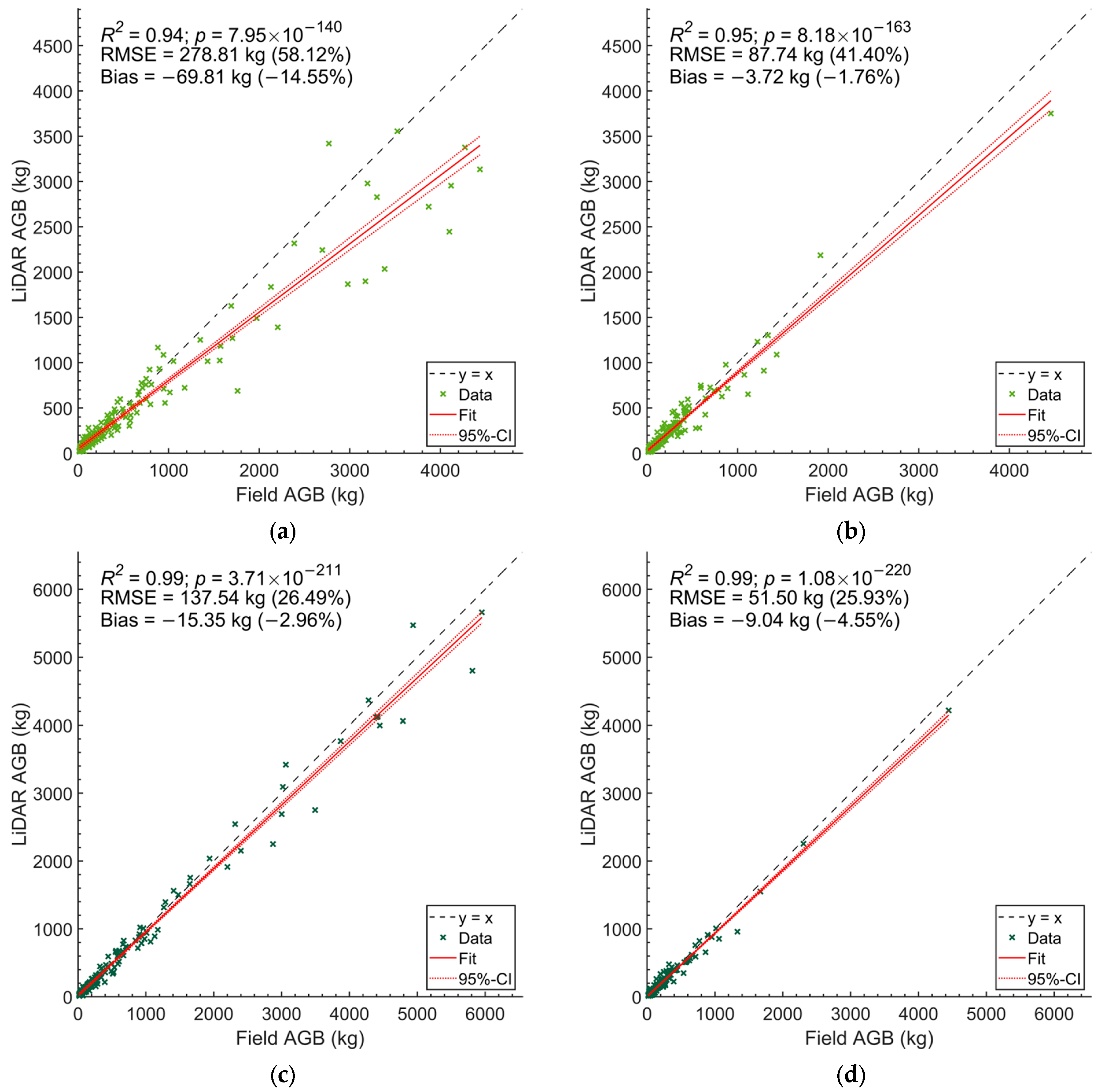
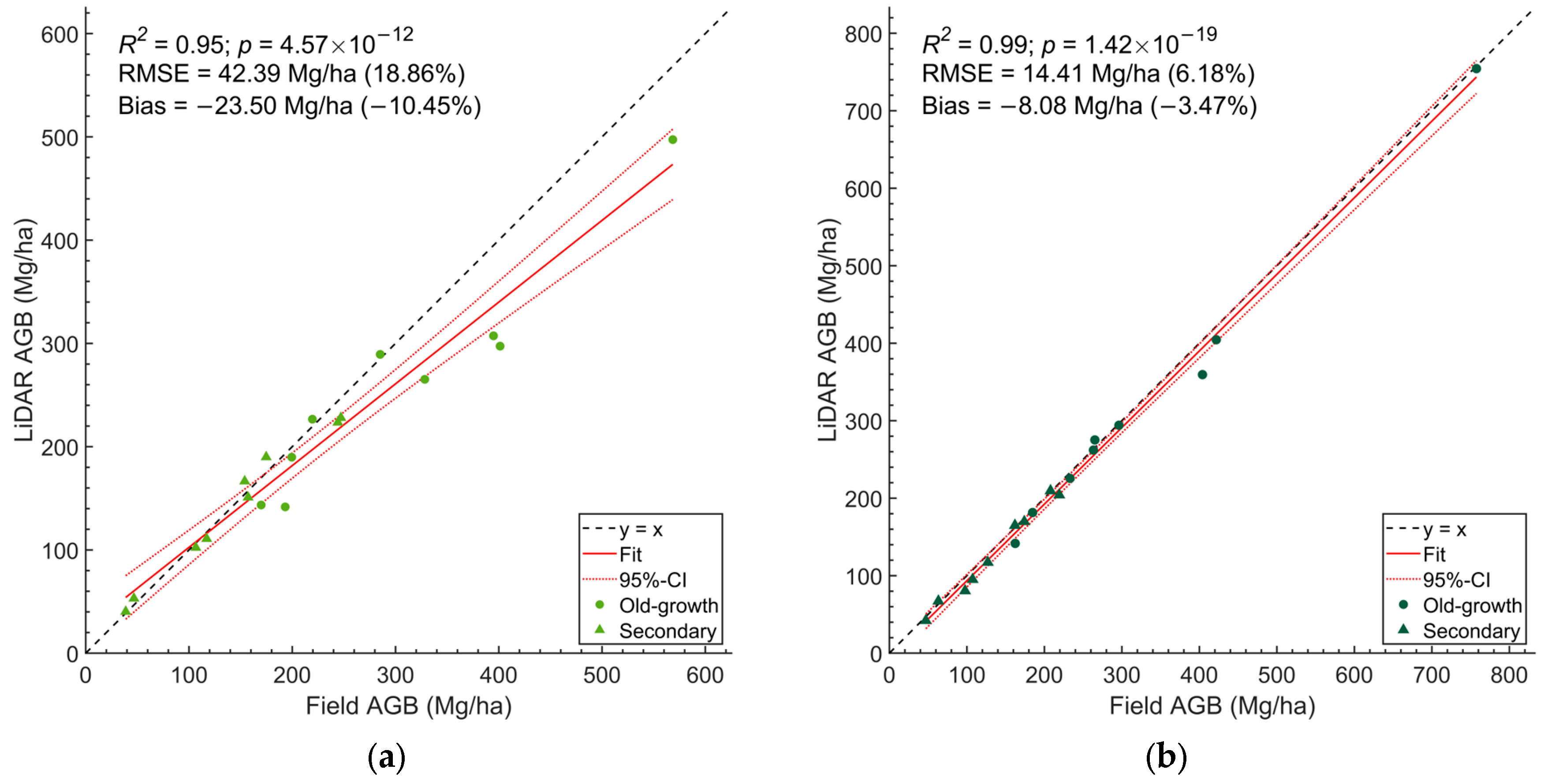
3.3. Estimating Individual Tree- and Plot-Level AGB in Old-Growth Forests and Secondary Forests

We estimated individual tree AGB using two different equations (Equations (5) and (6)) for both old-growth forests and secondary forests. Regardless of the equation used, there was a strong agreement between the AGB estimates from field data and those derived from HMLS, with R² values exceeding 0.94 in all cases. Overall, the equation that considered only DBH and specific wood density (Equation (6)) demonstrated better agreement than the equation that also included tree height (Equation (5)) (Figure 4).

For Equation (5), the agreement for old-growth forests decreased with increasing AGB values (R² = 0.94), exhibiting a bias of −14.6% and an RSME of 278.8 kg (58.1%) (Figure 4a). In contrast, in secondary forests, the HMLS-derived AGB estimate showed better alignment with field measurements (R² = 0.95), with an RMSE of 87.7 kg (41.4%) and a bias of −1.7% (Figure 4b). These patterns were consistent with Equation (6), where the agreement between HMLS and field data had an RMSE of 137.5 kg (26.5%) and a bias of −3.0% in old-growth forests, and an RMSE of 51.5 kg (25.9%) and a bias of −4.6% in secondary forests (Figure 4c,d).

Moreover, we compared the plot-level AGB of trees (DBH ≥ 9.5 cm) derived from HMLS with those from field data, excluding shrubs. Regardless of the equations used, old-growth forests stored more AGB than secondary forests (Figure 5). However, the HMLS estimates based on Equation (5) showed a larger negative bias compared to Equation (6) (Figure 5).

A summary of plot-level AGB estimations based on both equations for field data and HMLS is presented in

Table 4. Summary of aboveground biomass estimates for sampling plots in old-growth forests and secondary forests.

	Aboveground Biomass (Mg/ha)
	Old-Growth Forests		Secondary Forests
	Equation (5)	Equation (6)	Equation (5)	Equation (6)
Field data (trees and shrubs)	316.5 ± 131.7	340.2 ± 182.2	151.1 ± 76.4	140.6 ± 62.7
Field data (trees)	306.7 ± 130.8	332 ± 182	142.9 ± 74.6	134 ± 61
HMLS data (trees)	262 ± 108.6	322 ± 181.4	140.6 ± 68.7	127.8 ± 61.3
Average of field and HMLS (trees)	305.7 ± 30.9		136.3 ± 6.8

. In old-growth forests, the HMLS-derived estimates averaged 262.0 Mg/ha (Equation (5)) and 322.0 Mg/ha (Equation (6)). In secondary forests, the HMLS-derived estimates averaged 140.6 Mg/ha (Equation (5)) and 127.8 Mg/ha (Equation (6)). Based on field surveys, the average plot-level AGB was 306.7 Mg/ha AGB in old-growth forests, and 142.9 Mg/ha in secondary forests (Equation (5)). Additionally, we observed that including shrubs in the field data increased the plot-level AGB by 3.11% in old-growth forests and 5.39% in secondary forests.

4. Discussion

4.1. Tree Detection Capability

The HMLS system demonstrated a high capability for detecting trees in structurally complex subtropical forests, achieving detection rates of 90.6% in old-growth forests and 96.4% in secondary forests. These results are commendable given the challenging conditions during data collection, including closed canopy and high stem densities [74], which could reach up to 9550 stems/ha (Table 4). A study proposed complexity categories with a mean stem density of stems larger than 5 cm of 2130 stems/ha as a difficult scenario [75]. In our study, stem densities reached 2525 stems/ha (considering all stems ≥ 1 cm) in secondary forests and 9550 stems/ha in old-growth forests, all of which can be comparable to the difficult category as identified in prior studies.

Factors affecting detection accuracy included misclassification of points and the presence of lianas. For example, tilted trees, which lean to resist wind pressure or maintain stability on slopes [76], often intersect with surrounding trees in the point cloud. This complicates auto-segmentation due to clusters of points shared by multiple trees (Figure S3). Additionally, the presence of lianas can hinder the HMLS’s ability to scan the top canopy layer, causing occlusion effects and incomplete point clusters (Figure S4). Notably, the greater prevalence of lianas in old-growth forests compared to secondary forests likely contributed to the relatively lower tree detection rate in old-growth forests. A large coverage of shrubs and the slope of the terrain may also lead to a lower detection rate of trees [77].

Notably, LiDAR trajectories such as double and triple Z patterns and figure-eight loops have been tested in other studies [65]. For sensor optimization, we experimented with different scan paths within a square plot. Initially, we attempted to scan the plot using a path composed of four 5 m × 20 m horizontal rectangles joined by a diagonal path between the starting point and the ending point. However, this scan path proved to be too long, and the point cloud could not be successfully reconstructed. Consequently, we opted for the current double-Z configuration, which includes only four loops. This configuration avoids overly long or complex scan paths, ensuring successful point cloud reconstruction. Future research may consider modified scan paths such as integrated figure-eight loops that yield higher point cloud density and reduce occlusion effects [66].

Despite these challenges, the current study relied on manual input of field GPS as seed points for tree detection, which was time-consuming [78]. Future research could explore the application of deep learning for automated tree detection in complex forests [79]. Refined segmentation by defining tree boundaries and back-projections of 2D images can further improve tree detection by filtering out small trees [80]. Deep learning tools may be employed to enhance tree segmentation [78] and canopy detection [81]. Additionally, the methodology should be tested on more varied terrains, including uneven ground and steeper slopes [82], or in different habitats such as grasslands and shrublands [83,84]. Implementing a terrain-adaptive protocol may be beneficial for addressing the challenges posed by complex terrains [85,86].

4.2. Accuracy of Individual Tree Attribute Extraction

Our study demonstrated that forest attributes, such as the DBH of individual trees, can be accurately extracted from HMLS point clouds. The bias in extracting DBH from HMLS data compared to field data was less than ±2% (Figure 3). This indicates that HMLS measurements are comparable with field data, consistent with other terrestrial LiDAR systems [87,88]. To increase the accuracy of DBH estimation, it was suggested that a minimum threshold of HMLS coverage should be set [89]. Moreover, measuring the DBH of trees with convex buttress roots using standard dendrometrical tools resulted in overestimation compared to a smaller circle for DBH measurement detected from LiDAR360 [90] (Figure S5). The estimation of volume and biomass of trees is also affected by hollow or irregularly shaped trunks [91].

However, HMLS-derived tree heights were less accurate compared to field survey data (Figure 5). Although the algorithm accurately segmented most trees in the point cloud to their corresponding trees in the field, the derived height (highest point of the segmented tree) did not yield values comparable to survey data. HMLS tends to underestimate tree heights under complex canopy structures and tall canopies because laser penetration is obstructed by dense foliage [92]. Our analysis showed a negative bias in the estimation of tree height in both old-growth forests and secondary forests. The laser beam from ground scanning may not reach the tree top, leading to incomplete data from point clouds in that area [79].

Nevertheless, field measurements also have limitations, and may underestimate tree height due to limited visibility from the forest understory [93]. A study found average standard deviations of tree height measurements ranging from 0.41 m for trees between 15 m and 20 m, and 0.29 m for trees between 30 m and 35 m, due to instrumental or human error such as misidentification of the tree top [93]. Another study found the standard deviation to be 0.5 m (2.9% of the average tree height in the study) in dense forests due to reduced visibility of the tree top [94]. Uneven-aged forests with high canopy density present additional challenges in tree height measurements [75,95], as it is difficult to see and accurately measure the distance to the top of the surveyed trees. While efforts were made to minimize this uncertainty in the field by taking multiple height readings per tree, some uncertainty remains. Thus, determining the accuracy of HMLS- or field-derived tree height measurements requires independent verification methods, such as directly measuring felled trees. In our case, the structurally complex old-growth forests led to a higher likelihood of observational errors, resulting in a lower agreement between HMLS- and field-derived height estimations compared to secondary forests. A combination of TLS and ALS may address the limitation in tree height estimation by point-to-point matching of TLS and ALS trunk point clouds to achieve better accuracy [96,97,98].

4.3. Ability to Estimate AGB in Two Different Forest Types

Using forest attributes derived from the HMLS point clouds, we calculated both individual tree- and plot-level AGB in old-growth forests and secondary forests. Overall, the application of HMLS for estimating AGB showed significant correlation with field measurements (R² > 0.94) for both allometric equations (Equations (5) and (6)). The allometric equation using DBH and wood density alone (Equation (6)) provided consistent results between HMLS- and field-derived AGB in both forest types. However, estimates based on the equation considering tree heights (Equation (5)) showed greater discrepancy due to the higher susceptibility of height estimations to measurement errors. This discrepancy is further amplified in old-growth forests where larger, taller trees and higher stem densities in a plot, combined with thicker canopy layers, potentially caused occlusions. This, in turn, reduced the agreement between HMLS- and field-derived AGB estimates for this forest type. Conversely, in secondary forests, the AGB estimates from HMLS showed better agreement with field data, with a bias of less than 5% at both the individual and plot levels.

Based on the survey findings, old-growth forests have significantly higher AGB compared to secondary forests. Utilizing the IPCC conversion standard of 0.47, it is estimated that old-growth forests have an average AGB of 305.7 Mg/ha equivalent to 143.7 MgC/ha, whereas secondary forests contain 64.2 MgC/ha [10]. This stark contrast underscores the crucial role of old-growth forests as vital carbon sinks [99,100]. It is concerning that many old-growth forests in Hong Kong currently lack statutory protection [101]. Preserving these forests not only contributes to carbon sequestration but also plays a pivotal role in maintaining biodiversity and ecosystem health. It is important to protect local forests as nature-based solutions against climate change, and the AGB estimates would serve as baseline data for regional climate mitigation plans.

Our study highlights that large-sized trees store significantly more carbon than small trees, which concurs with the well-established finding in the literature [102]. However, our results provide new data for the Hong Kong SAR Government, indicating that the current policy on compensating tree and forest loss during urban development is insufficient. The current policy mandates a minimum compensatory tree planting ratio of 1 to 1 in terms of the number of trees, i.e., the number of compensatory trees planted on-site or off-site should not be smaller than the number of trees removed [103]. Often, large trees removed are compensated for by planting young trees, resulting in significant carbon loss. Meanwhile, our results suggest that old-growth forests are crucial for carbon storage. These old-growth forests in Hong Kong, known as Fung Shui Woods, are important for harboring many unique lowland tree and plant species [57]. There are over 100 Fung Shui Woods in Hong Kong, most of which are unprotected. The results of this study should prompt the Government to review the carbon sequestration potential of these old-growth forests and designate them as protected areas, such as Green Belt, Site of Special Scientific Interest (SSSI), or Conservation Area [104].

4.4. Limitations of This Study

While HMLS point clouds offer an efficient and time-saving method to derive individual tree structural metrics, accurate tree segmentation remains a significant challenge. In complex subtropical forests, classifying overlapping small branches often requires human intervention [105,106]. Imperfect delineation reduces the accuracy of estimated canopy structural attributes, such as tree height and crown area, impacting subsequent analyses. Additionally, without physically cutting down trees for measurement, obtaining the actual heights and volumes of the trees is impossible. Hence, we cannot fully verify the accuracy of height estimates from both HMLS and field measurements. Moreover, the AGB estimates were based on allometric equations developed for tropical broad-leaved forests by Chave et al. [9]. Our comparison of two allometric equations revealed higher estimated biomass using Equation (6) based on DBH compared to Equation (5). Although there is one local allometric equation from Hong Kong, the dataset was derived from a mix of exotic and native species [20,107] and may not fully represent native forests. We conducted a sensitivity analysis, which showed biomass estimates using equations from Hong Kong, Guangdong, and Taiwan [20,21,22] to be highly correlated at the tree level but showing the plot-level bias (Figure S5). Among the 61 species recorded in this study, only 11 species had species-specific allometric equations recorded in the dataset of tree biomass equations for China [18,19]. As there is no forestry activity in Hong Kong, obtaining the dry mass of native species and developing local species-specific allometric equations is challenging. Future studies should coordinate with large Government initiatives (e.g., carbon neutrality action plans) to develop specific allometric equations for the forests in Hong Kong. Furthermore, integrating ALS with HMLS should be explored to obtain more accurate height information of individual trees and canopy tree crown areas to refine AGB estimation results.

5. Conclusions

This study evaluates the effectiveness of Handheld Mobile Laser Scanning (HMLS) for tree detection, forest attribute extraction, and AGB estimation across different forest types in subtropical Hong Kong. Our results demonstrate that HMLS is highly effective, successfully segmenting and detecting over 90% of trees within sampling plots in both old-growth and secondary forests. The measurements of DBH from HMLS point clouds proved reliable in both forest types. However, we observed relatively greater discrepancies in height detection. For AGB estimation, we employed two allometric equations designed for tropical trees. Our results indicate that HMLS can effectively estimate AGB in less complex forest environments. Notably, in structurally complex environments like old-growth forests, using an allometric equation that excludes the height attribute resulted in an improved agreement between HMLS- and field-derived estimates. Collectively, these findings suggest that HMLS is an effective and non-destructive tool for estimating AGB in forest plots, significantly reducing the time required for on-site tree surveys. Further research should focus on developing an allometric equation tailored to the forests of Hong Kong, incorporating both DBH and height to enhance the accuracy of local AGB estimations.

References

1. Melo, F.P.L.; Parry, L.; Brancalion, P.H.S.; Pinto, S.R.R.; Freitas, J.; Manhães, A.P.; Meli, P.; Ganade, G.; Chazdon, R.L. Adding forests to the water–energy–food nexus. Nat. Sustain. 2021, 4, 85–92. [Google Scholar] [CrossRef]
2. Law, B.E.; Berner, L.T.; Buotte, P.C.; Mildrexler, D.J.; Ripple, W.J. Strategic Forest Reserves can protect biodiversity in the western United States and mitigate climate change. Commun. Earth Environ. 2021, 2, 254. [Google Scholar] [CrossRef]
3. Triviño, M.; Morán-Ordoñez, A.; Eyvindson, K.; Blattert, C.; Burgas, D.; Repo, A.; Pohjanmies, T.; Brotons, L.; Snäll, T.; Mönkkönen, M. Future supply of boreal forest ecosystem services is driven by management rather than by climate change. Glob. Change Biol. 2023, 29, 1484–1500. [Google Scholar] [CrossRef] [PubMed]
4. Capellesso, E.S.; Cequinel, A.; Marques, R.; Sausen, T.L.; Bayer, C.; Marques, M.C.M. Co-benefits in biodiversity conservation and carbon stock during forest regeneration in a preserved tropical landscape. For. Ecol. Manag. 2021, 492, 119222. [Google Scholar] [CrossRef]
5. Mukul, S.A.; Halim, M.A.; Herbohn, J. Forest carbon stock and fluxes: Distribution, biogeochemical cycles, and measurement techniques. In Life on Land; Encyclopedia of the UN Sustainable Development Goals; Springer: Cham, Switzerland, 2020; pp. 365–380. [Google Scholar]
6. Zhao, J.; Liu, D.; Zhu, Y.; Peng, H.; Xie, H. A review of forest carbon cycle models on spatiotemporal scales. J. Clean. Prod. 2022, 339, 130692. [Google Scholar] [CrossRef]
7. Raihan, A.; Begum, R.A.; Mohd Said, M.N.; Pereira, J.J. Assessment of carbon stock in forest biomass and emission reduction potential in Malaysia. Forests 2021, 12, 1294. [Google Scholar] [CrossRef]
8. Siddiq, Z.; Hayyat, M.U.; Khan, A.U.; Mahmood, R.; Shahzad, L.; Ghaffar, R.; Cao, K.-F. Models to estimate the above and below ground carbon stocks from a subtropical scrub forest of Pakistan. Glob. Ecol. Conserv. 2021, 27, e01539. [Google Scholar] [CrossRef]
9. Chave, J.; Réjou-Méchain, M.; Búrquez, A.; Chidumayo, E.; Colgan, M.S.; Delitti, W.B.C.; Duque, A.; Eid, T.; Fearnside, P.M.; Goodman, R.C.; et al. Improved allometric models to estimate the aboveground biomass of tropical trees. Glob. Change Biol. 2014, 20, 3177–3190. [Google Scholar] [CrossRef]
10. Rozendaal, D.M.A.; Requena Suarez, D.; De Sy, V.; Avitabile, V.; Carter, S.; Adou Yao, C.Y.; Alvarez-Davila, E.; Anderson-Teixeira, K.; Araujo-Murakami, A.; Arroyo, L.; et al. Aboveground forest biomass varies across continents, ecological zones and successional stages: Refined IPCC default values for tropical and subtropical forests. Environ. Res. Lett. 2022, 17, 014047. [Google Scholar] [CrossRef]
11. Zeng, N.; Jiang, K.; Han, P.; Hausfather, Z.; Cao, J.; Kirk-Davidoff, D.; Ali, S.; Zhou, S. The Chinese carbon-neutral goal: Challenges and prospects. Adv. Atmos. Sci. 2022, 39, 1229–1238. [Google Scholar] [CrossRef]
12. Brown, S.; Gillespie, A.J.R.; Lugo, A.E. Biomass estimation methods for tropical forests with applications to forest inventory data. For. Sci. 1989, 35, 881–902. [Google Scholar] [CrossRef]
13. Chave, J.; Andalo, C.; Brown, S.; Cairns, M.A.; Chambers, J.Q.; Eamus, D.; Fölster, H.; Fromard, F.; Higuchi, N.; Kira, T.; et al. Tree allometry and improved estimation of carbon stocks and balance in tropical forests. Oecologia 2005, 145, 87–99. [Google Scholar] [CrossRef] [PubMed]
14. Vashum, K.T.; Jayakumar, S. Methods to estimate above-ground biomass and carbon stock in natural forests-a review. J. Ecosyst. Ecography 2012, 2, 116. [Google Scholar] [CrossRef]
15. Zhuang, X.Y. Forest succession in Hong Kong. Ph.D. Thesis, University of Hong Kong, Hong Kong, China, 1993. [Google Scholar]
16. Gonzalez-Akre, E.; Piponiot, C.; Lepore, M.; Herrmann, V.; Lutz, J.A.; Baltzer, J.L.; Dick, C.W.; Gilbert, G.S.; He, F.; Heym, M.; et al. allodb: An R package for biomass estimation at globally distributed extratropical forest plots. Methods Ecol. Evol. 2022, 13, 330–338. [Google Scholar] [CrossRef]
17. Harja, D.; Rahayu, S.; Pambudi, S. Tree Functional Attributes and Ecological Database. World Agroforestry Centre (ICRAF), Nairobi. 2018. Available online: https://www.worldagroforestry.org/output/tree-functional-and-ecological-databases (accessed on 15 August 2022).
18. Luo, Y.; Wang, X.; Ouyang, Z. A China’s Normalized Tree Biomass Equation Dataset [Dataset]. PANGAEA 2018. [Google Scholar] [CrossRef]
19. Luo, Y.; Wang, X.; Ouyang, Z.; Lu, F.; Feng, L.; Tao, J. A review of biomass equations for China’s tree species. Earth Syst. Sci. Data 2020, 12, 21–40. [Google Scholar] [CrossRef]
20. Nichol, J.E.; Sarker, M.L.R. Improved biomass estimation using the texture parameters of two high-resolution optical sensors. IEEE Trans. Geosci. Remote Sens. 2010, 49, 930–948. [Google Scholar] [CrossRef]
21. Zhao, H.; Li, Z.; Zhou, G.; Qiu, Z.; Wu, Z. Site-specific allometric models for prediction of above-and belowground biomass of subtropical forests in Guangzhou, southern China. Forests 2019, 10, 862. [Google Scholar] [CrossRef]
22. Lin, K.C.; Ma, F.C.; Tang, S.L. Allometric Equations for Predicting the Aboveground Biomass of Tree Species in the Fushan Forest. Taiwan J. For. Sci. 2001, 16, 143–151. [Google Scholar] [CrossRef]
23. Gallaun, H.; Zanchi, G.; Nabuurs, G.-J.; Hengeveld, G.; Schardt, M.; Verkerk, P.J. EU-wide maps of growing stock and above-ground biomass in forests based on remote sensing and field measurements. For. Ecol. Manag. 2010, 260, 252–261. [Google Scholar] [CrossRef]
24. Zellweger, F.; Morsdorf, F.; Purves, R.S.; Braunisch, V.; Bollmann, K. Improved methods for measuring forest landscape structure: LiDAR complements field-based habitat assessment. Biodivers. Conserv. 2014, 23, 289–307. [Google Scholar] [CrossRef]
25. Wulder, M.A.; White, J.C.; Nelson, R.F.; Næsset, E.; Ørka, H.O.; Coops, N.C.; Hilker, T.; Bater, C.W.; Gobakken, T. Lidar sampling for large-area forest characterization: A review. Remote Sens. Environ. 2012, 121, 196–209. [Google Scholar] [CrossRef]
26. Almeida, D.R.A.D.; Stark, S.C.; Chazdon, R.; Nelson, B.W.; César, R.G.; Meli, P.; Gorgens, E.B.; Duarte, M.M.; Valbuena, R.; Moreno, V.S.; et al. The effectiveness of lidar remote sensing for monitoring forest cover attributes and landscape restoration. For. Ecol. Manag. 2019, 438, 34–43. [Google Scholar] [CrossRef]
27. Fuhr, M.; Lalechère, E.; Monnet, J.M.; Bergès, L. Detecting overmature forests with airborne laser scanning (ALS). Remote Sens. Ecol. Conserv. 2022, 8, 731–743. [Google Scholar] [CrossRef]
28. Newnham, G.J.; Armston, J.D.; Calders, K.; Disney, M.I.; Lovell, J.L.; Schaaf, C.B.; Strahler, A.H.; Danson, F.M. Terrestrial laser scanning for plot-scale forest measurement. Curr. For. Rep. 2015, 1, 239–251. [Google Scholar] [CrossRef]
29. Pascu, I.-S.; Dobre, A.-C.; Badea, O.; Tănase, M.A. Estimating forest stand structure attributes from terrestrial laser scans. Sci. Total Environ. 2019, 691, 205–215. [Google Scholar] [CrossRef]
30. Hirschmugl, M.; Lippl, F.; Sobe, C. Assessing the vertical structure of forests using airborne and spaceborne LiDAR data in the Austrian Alps. Remote Sens. 2023, 15, 664. [Google Scholar] [CrossRef]
31. Cosgrove, C.F.; Coops, N.C.; Martin, T.G. Using the full potential of Airborne Laser Scanning (aerial LiDAR) in wildlife research. Wildl. Soc. Bull. 2024, 48, e1532. [Google Scholar] [CrossRef]
32. Ma, K.; Chen, Z.; Fu, L.; Tian, W.; Jiang, F.; Yi, J.; Du, Z.; Sun, H. Performance and sensitivity of individual tree segmentation methods for UAV-LiDAR in multiple forest types. Remote Sens. 2022, 14, 298. [Google Scholar] [CrossRef]
33. Di Stefano, F.; Chiappini, S.; Gorreja, A.; Balestra, M.; Pierdicca, R. Mobile 3D scan LiDAR: A literature review. Geomat. Nat. Hazards Risk 2021, 12, 2387–2429. [Google Scholar] [CrossRef]
34. Lei, L.; Li, Z.; Wu, J.; Zhang, C.; Zhu, Y.; Chen, R.; Dong, Z.; Yang, H.; Yang, G. Extraction of maize leaf base and inclination angles using terrestrial laser scanning (TLS) data. IEEE Trans. Geosci. Remote Sens. 2022, 60, 1–17. [Google Scholar] [CrossRef]
35. Panagiotidis, D.; Abdollahnejad, A.; Slavík, M. 3D point cloud fusion from UAV and TLS to assess temperate managed forest structures. Int. J. Appl. Earth Obs. Geoinf. 2022, 112, 102917. [Google Scholar] [CrossRef]
36. Czimber, K.; Szász, B.; Ács, N.; Heilig, D.; Illés, G.; Mészáros, D.; Veperdi, G.; Heil, B.; Kovács, G. Estimation of the Total Carbon Stock of Dudles Forest Based on Satellite Imagery, Airborne Laser Scanning, and Field Surveys. Forests 2025, 16, 512. [Google Scholar] [CrossRef]
37. Thies, M.; Spiecker, H. Evaluation and future prospects of terrestrial laser scanning for standardized forest inventories. Forest 2004, 2, 192–197. [Google Scholar]
38. Wilkes, P.; Lau, A.; Disney, M.; Calders, K.; Burt, A.; de Tanago, J.G.; Bartholomeus, H.; Brede, B.; Herold, M. Data acquisition considerations for terrestrial laser scanning of forest plots. Remote Sens. Environ. 2017, 196, 140–153. [Google Scholar] [CrossRef]
39. Gollob, C.; Ritter, T.; Nothdurft, A. Forest inventory with long range and high-speed personal laser scanning (PLS) and simultaneous localization and mapping (SLAM) technology. Remote Sens. 2020, 12, 1509. [Google Scholar] [CrossRef]
40. Liang, X.; Kankare, V.; Hyyppä, J.; Wang, Y.; Kukko, A.; Haggrén, H.; Yu, X.; Kaartinen, H.; Jaakkola, A.; Guan, F.; et al. Terrestrial laser scanning in forest inventories. ISPRS J. Photogramm. Remote Sens. 2016, 115, 63–77. [Google Scholar] [CrossRef]
41. Kuželka, K.; Marušák, R.; Surový, P. Inventory of close-to-nature forest stands using terrestrial mobile laser scanning. Int. J. Appl. Earth Obs. Geoinf. 2022, 115, 103104. [Google Scholar] [CrossRef]
42. Vandendaele, B.; Martin-Ducup, O.; Fournier, R.A.; Pelletier, G.; Lejeune, P. Mobile laser scanning for estimating tree structural attributes in a temperate hardwood Forest. Remote Sens. 2022, 14, 4522. [Google Scholar] [CrossRef]
43. Ryding, J.; Williams, E.; Smith, M.J.; Eichhorn, M.P. Assessing handheld mobile laser scanners for forest surveys. Remote Sens. 2015, 7, 1095–1111. [Google Scholar] [CrossRef]
44. Bauwens, S.; Bartholomeus, H.; Calders, K.; Lejeune, P. Forest inventory with terrestrial LiDAR: A comparison of static and hand-held mobile laser scanning. Forests 2016, 7, 127. [Google Scholar] [CrossRef]
45. Vatandaşlar, C.; Zeybek, M. Extraction of forest inventory parameters using handheld mobile laser scanning: A case study from Trabzon, Turkey. Measurement 2021, 177, 109328. [Google Scholar] [CrossRef]
46. Bienert, A.; Georgi, L.; Kunz, M.; von Oheimb, G.; Maas, H.-G. Automatic extraction and measurement of individual trees from mobile laser scanning point clouds of forests. Ann. Bot. 2021, 128, 787–804. [Google Scholar] [CrossRef] [PubMed]
47. Fekry, R.; Yao, W.; Cao, L.; Shen, X. Ground-based/UAV-LiDAR data fusion for quantitative structure modeling and tree parameter retrieval in subtropical planted forest. For. Ecosyst. 2022, 9, 100065. [Google Scholar] [CrossRef]
48. Calders, K.; Adams, J.; Armston, J.; Bartholomeus, H.; Bauwens, S.; Bentley, L.P.; Chave, J.; Danson, F.M.; Demol, M.; Disney, M.; et al. Terrestrial laser scanning in forest ecology: Expanding the horizon. Remote Sens. Environ. 2020, 251, 112102. [Google Scholar] [CrossRef]
49. Mathes, T.; Seidel, D.; Häberle, K.-H.; Pretzsch, H.; Annighöfer, P. What are we missing? Occlusion in laser scanning point clouds and its impact on the detection of single-tree morphologies and stand structural variables. Remote Sens. 2023, 15, 450. [Google Scholar] [CrossRef]
50. Cheung, P.K.; Jim, C.Y.; Siu, C.T. Effects of urban park design features on summer air temperature and humidity in compact-city milieu. Appl. Geogr. 2021, 129, 102439. [Google Scholar] [CrossRef]
51. Law, Y.K.; Lee, C.K.F.; Pang, C.C.; Hau, B.C.H.; Wu, J. Vegetation regeneration on natural terrain landslides in Hong Kong: Direct seeding of native species as a restoration tool. Land Degrad. Dev. 2023, 34, 751–762. [Google Scholar] [CrossRef]
52. Law, Y.K.; Lee, C.K.F.; Chan, A.H.Y.; Mak, N.P.L.; Hau, B.C.H.; Wu, J. Unveiling the role of forests in landslide occurrence, recurrence and recovery. J. Appl. Ecol. 2024, 61, 2033–2046. [Google Scholar] [CrossRef]
53. Kwong, I.H.Y.; Wong, F.K.K.; Fung, T.; Liu, E.K.Y.; Lee, R.H.; Ng, T.P.T. A multi-stage approach combining very high-resolution satellite image, gis database and post-classification modification rules for habitat mapping in Hong Kong. Remote Sens. 2021, 14, 67. [Google Scholar] [CrossRef]
54. Corlett, R.T. Environmental forestry in Hong Kong: 1871–1997. For. Ecol. Manag. 1999, 116, 93–105. [Google Scholar] [CrossRef]
55. Zhang, H.; Lee, C.K.F.; Law, Y.K.; Chan, A.H.Y.; Zhang, J.; Gale, S.W.; Hughes, A.; Ledger, M.J.; Wong, M.S.; Tai, A.P.K.; et al. Integrating both restoration and regeneration potentials into real-world forest restoration planning: A case study of Hong Kong. J. Environ. Manag. 2024, 369, 122306. [Google Scholar] [CrossRef] [PubMed]
56. Hong Kong Herbarium. An Overview of Fung Shui Woods in Hong Kong. Available online: https://www.herbarium.gov.hk/en/special-topics/fung-shui-woods/an-overview-of-fung-shui-woods-in-hong-kong/index.html (accessed on 10 February 2024).
57. Yip, J.K.L.; Ngar, Y.N.; Yip, J.Y.; Liu, E.K.Y.; Lai, P.C.C. Venturing Fung Shui Woods; Friends of the Country Parks, Agriculture, Fisheries and Conservation Department & Cosmos Books Ltd.: Hong Kong, China, 2004. [Google Scholar]
58. Chen, B.; Coggins, C.; Minor, J.; Zhang, Y. Fengshui forests and village landscapes in China: Geographic extent, socioecological significance, and conservation prospects. Urban For. Urban Green. 2018, 31, 79–92. [Google Scholar] [CrossRef]
59. Zhuang, X.Y.; Gorlett, R.T. Forest and forest succession in Hong Kong, China. J. Trop. Ecol. 1997, 13, 857–866. [Google Scholar] [CrossRef]
60. Hu, L.; Li, Z.; Liao, W.-B.; Fan, Q. Values of village fengshui forest patches in biodiversity conservation in the Pearl River Delta, China. Biol. Conserv. 2011, 144, 1553–1559. [Google Scholar] [CrossRef]
61. Zhu, H.; Zhang, J.; Hau, B.C.H.; Shum, B.T.W.; Ma, X.K.K.; Lo, J.P.L.; Fischer, G.A.; Gale, S.W. Tai Po Kau ForestGEO Forest Dynamics Plot: Species Composition and Community Structure; Kadoorie Farm and Botanic Garden: Hong Kong, China, 2024. [Google Scholar]
62. Nicholson, B. Tai Po Kau nature reserve, new territories, Hong Kong: A reafforestation history. Asian J. Environ. Manag. 1996, 4, 103–120. [Google Scholar]
63. Condit, R. Tropical Forest Census Plots: Methods and Results from Barro Colorado Island, Panama and a Comparison with Other Plots; Springer: Berlin/Heidelberg, Germany, 1998. [Google Scholar]
64. GreenValley International. LiGrip H120 Rotating Handheld SLAM LiDAR System Quick Start Manual. Available online: https://www.greenvalleyintl.com/gvi/web/us/file/EN-LiGripH120-UserManual-(Ver-A.10).pdf (accessed on 22 December 2024).
65. Su, Y.; Guo, Q.; Jin, S.; Guan, H.; Sun, X.; Ma, Q.; Hu, T.; Wang, R.; Li, Y. The development and evaluation of a backpack LiDAR system for accurate and efficient forest inventory. IEEE Geosci. Remote Sens. Lett. 2020, 18, 1660–1664. [Google Scholar] [CrossRef]
66. Li, L.; Wei, L.; Li, N.; Zhang, S.; Hu, M.; Ma, J. Impact of Backpack LiDAR Scan Routes on Diameter at Breast Height Estimation in Forests. Forests 2025, 16, 527. [Google Scholar] [CrossRef]
67. GreenValley International. LiFuser-BP Data Fusion Software User Guide. Available online: https://www.greenvalleyintl.com/static/upload/file/20231215/1702625843211308.pdf (accessed on 30 December 2024).
68. Zhao, X.; Guo, Q.; Su, Y.; Xue, B. Improved progressive TIN densification filtering algorithm for airborne LiDAR data in forested areas. ISPRS J. Photogramm. Remote Sens. 2016, 117, 79–91. [Google Scholar] [CrossRef]
69. Tao, S.; Wu, F.; Guo, Q.; Wang, Y.; Li, W.; Xue, B.; Hu, X.; Li, P.; Tian, D.; Li, C.; et al. Segmenting tree crowns from terrestrial and mobile LiDAR data by exploring ecological theories. ISPRS J. Photogramm. Remote Sens. 2015, 110, 66–76. [Google Scholar] [CrossRef]
70. MATLAB, version: 9.13.0 (R2022b); The MathWorks Inc.: Natick, MA, USA, 2022.
71. Chao, K.; Li, Y.; Song, G.M.; Chao, W.; Chang-Yang, C.; Chiang, J. Database for Carbon Stocks Estimation Variables of Tree Species Used in Soil and Water Conservation. J. Chin. Soil Water Conserv. 2024, 53, 100–110. [Google Scholar] [CrossRef]
72. Chave, J.; Coomes, D.; Jansen, S.; Lewis, S.L.; Swenson, N.G.; Zanne, A.E. Towards a worldwide wood economics spectrum. Ecol. Lett. 2009, 12, 351–366. [Google Scholar] [CrossRef] [PubMed]
73. Zanne, A.E.; Lopez-Gonzalez, G.; Coomes, D.A.; Ilic, J.; Jansen, S.; Lewis, S.L.; Miller, R.B.; Swenson, N.G.; Wiemann, M.C.; Chave, J. Data from: Towards a worldwide wood economics spectrum [dataset]. Dryad 2009. [Google Scholar] [CrossRef]
74. Tupinambá-Simões, F.; Pascual, A.; Guerra-Hernández, J.; Ordóñez, C.; de Conto, T.; Bravo, F. Assessing the performance of a handheld laser scanning system for individual tree mapping—A Mixed forests showcase in Spain. Remote Sens. 2023, 15, 1169. [Google Scholar] [CrossRef]
75. Wang, Y.; Lehtomäki, M.; Liang, X.; Pyörälä, J.; Kukko, A.; Jaakkola, A.; Liu, J.; Feng, Z.; Chen, R.; Hyyppä, J. Is field-measured tree height as reliable as believed–A comparison study of tree height estimates from field measurement, airborne laser scanning and terrestrial laser scanning in a boreal forest. ISPRS J. Photogramm. Remote Sens. 2019, 147, 132–145. [Google Scholar] [CrossRef]
76. Jim, C.Y. Soil compaction as a constraint to tree growth in tropical & subtropical urban habitats. Environ. Conserv. 1993, 20, 35–49. [Google Scholar]
77. Kükenbrink, D.; Marty, M.; Rehush, N.; Abegg, M.; Ginzler, C. Evaluating the potential of handheld mobile laser scanning for an operational inclusion in a national forest inventory—A Swiss case study. Remote Sens. Environ. 2025, 321, 114685. [Google Scholar] [CrossRef]
78. Henrich, J.; van Delden, J.; Seidel, D.; Kneib, T.; Ecker, A.S. TreeLearn: A deep learning method for segmenting individual trees from ground-based LiDAR forest point clouds. Ecol. Inform. 2024, 84, 102888. [Google Scholar] [CrossRef]
79. Itakura, K.; Miyatani, S.; Hosoi, F. Estimating tree structural parameters via automatic tree segmentation from LiDAR point cloud data. IEEE J. Sel. Top. Appl. Earth Obs. Remote Sens. 2021, 15, 555–564. [Google Scholar] [CrossRef]
80. Chang, L.; Fan, H.; Zhu, N.; Dong, Z. A two-stage approach for individual tree segmentation from TLS point clouds. IEEE J. Sel. Top. Appl. Earth Obs. Remote Sens. 2022, 15, 8682–8693. [Google Scholar] [CrossRef]
81. Xu, J.; Zhang, Z.; Hu, X.; Ke, T. Accelerated forest modeling from tree canopy point clouds via deep learning. Int. J. Appl. Earth Obs. Geoinf. 2024, 132, 104074. [Google Scholar] [CrossRef]
82. Sofia, S.; Sferlazza, S.; Mariottini, A.; Niccolini, M.; Coppi, T.; Miozzo, M.; La Mantia, T.; Maetzke, F. A case study of the application of hand-held mobile laser scanning in the planning of an italian forest (Alpe di Catenaia, Tuscany). Int. Arch. Photogramm. Remote Sens. Spat. Inf. Sci. 2021, XLIII-B2-2021, 763–770. [Google Scholar] [CrossRef]
83. de Nobel, J.S.; Rijsdijk, K.F.; Cornelissen, P.; Seijmonsbergen, A.C. Towards Prediction and Mapping of Grassland Aboveground Biomass Using Handheld LiDAR. Remote Sens. 2023, 15, 1754. [Google Scholar] [CrossRef]
84. Li, M.; Li, Z.; Zhang, M.; Liu, Q.; Li, M. Efficient shrub modelling based on terrestrial laser scanning (TLS) point clouds. Int. J. Remote Sens. 2024, 45, 1148–1169. [Google Scholar] [CrossRef]
85. Wang, B.; Wang, H.; Song, D. A filtering method for LiDAR point cloud based on multi-scale CNN with attention mechanism. Remote Sens. 2022, 14, 6170. [Google Scholar] [CrossRef]
86. Cai, S.; Yu, S. Filtering airborne LiDAR data in forested environments based on multi-directional narrow window and cloth simulation. Remote Sens. 2023, 15, 1400. [Google Scholar] [CrossRef]
87. Hyyppä, E.; Yu, X.; Kaartinen, H.; Hakala, T.; Kukko, A.; Vastaranta, M.; Hyyppä, J. Comparison of backpack, handheld, under-canopy UAV, and above-canopy UAV laser scanning for field reference data collection in boreal forests. Remote Sens. 2020, 12, 3327. [Google Scholar] [CrossRef]
88. Stal, C.; Verbeurgt, J.; De Sloover, L.; De Wulf, A. Assessment of handheld mobile terrestrial laser scanning for estimating tree parameters. J. For. Res. 2021, 32, 1503–1513. [Google Scholar] [CrossRef]
89. Čerňava, J.; Tuček, J.; Koreň, M.; Mokroš, M. Estimation of diameter at breast height from mobile laser scanning data collected under a heavy forest canopy. J. For. Sci. 2017, 63, 433–441. [Google Scholar] [CrossRef]
90. Ngomanda, A.; Mavouroulou, Q.M.; Obiang, N.L.E.; Iponga, D.M.; Mavoungou, J.-F.; Lépengué, N.; Picard, N.; Mbatchi, B. Derivation of diameter measurements for buttressed trees, an example from Gabon. J. Trop. Ecol. 2012, 28, 299–302. [Google Scholar] [CrossRef]
91. Nogueira, E.M.; Nelson, B.W.; Fearnside, P.M. Volume and biomass of trees in central Amazonia: Influence of irregularly shaped and hollow trunks. For. Ecol. Manag. 2006, 227, 14–21. [Google Scholar] [CrossRef]
92. Lin, Y.; Hyyppä, J.; Jaakkola, A.; Yu, X. Three-level frame and RD-schematic algorithm for automatic detection of individual trees from MLS point clouds. Int. J. Remote Sens. 2012, 33, 1701–1716. [Google Scholar] [CrossRef]
93. Jurjević, L.; Liang, X.; Gašparović, M.; Balenović, I. Is field-measured tree height as reliable as believed–Part II, A comparison study of tree height estimates from conventional field measurement and low-cost close-range remote sensing in a deciduous forest. ISPRS J. Photogramm. Remote Sens. 2020, 169, 227–241. [Google Scholar] [CrossRef]
94. Luoma, V.; Saarinen, N.; Wulder, M.A.; White, J.C.; Vastaranta, M.; Holopainen, M.; Hyyppä, J. Assessing precision in conventional field measurements of individual tree attributes. Forests 2017, 8, 38. [Google Scholar] [CrossRef]
95. Fan, Y.; Feng, Z.; Mannan, A.; Khan, T.U.; Shen, C.; Saeed, S. Estimating tree position, diameter at breast height, and tree height in real-time using a mobile phone with RGB-D SLAM. Remote Sens. 2018, 10, 1845. [Google Scholar] [CrossRef]
96. Chen, J.; Zhao, D.; Zheng, Z.; Xu, C.; Pang, Y.; Zeng, Y. A clustering-based automatic registration of UAV and terrestrial LiDAR forest point clouds. Comput. Electron. Agric. 2024, 217, 108648. [Google Scholar] [CrossRef]
97. Deng, Y.; Wang, J.; Dong, P.; Liu, Q.; Ma, W.; Zhang, J.; Su, G.; Li, J. Registration of TLS and ULS Point Cloud Data in Natural Forest Based on Similar Distance Search. Forests 2024, 15, 1569. [Google Scholar] [CrossRef]
98. Gan, Y.; Wang, Q.; Song, G. Non-Destructive Estimation of Deciduous Forest Metrics: Comparisons between UAV-LiDAR, UAV-DAP, and Terrestrial LiDAR Leaf-Off Point Clouds Using Two QSMs. Remote Sens. 2024, 16, 697. [Google Scholar] [CrossRef]
99. Luyssaert, S.; Schulze, E.D.; Börner, A.; Knohl, A.; Hessenmöller, D.; Law, B.E.; Ciais, P.; Grace, J. Old-growth forests as global carbon sinks. Nature 2008, 455, 213–215. [Google Scholar] [CrossRef]
100. Harmon, M.E.; Ferrell, W.K.; Franklin, J.F. Effects on carbon storage of conversion of old-growth forests to young forests. Science 1990, 247, 699–702. [Google Scholar] [CrossRef]
101. Lee, K.W.K.; Cheuk, M.L.; Fischer, G.A.; Gale, S.W. Can Disparate Shared Social Values Benefit the Conservation of Biodiversity in Hong Kong’s Sacred Groves? Hum. Ecol. 2023, 51, 1021–1032. [Google Scholar] [CrossRef]
102. Lutz, J.A.; Furniss, T.J.; Johnson, D.J.; Davies, S.J.; Allen, D.; Alonso, A.; Anderson-Teixeira, K.J.; Andrade, A.; Baltzer, J.; Becker, K.M.L.; et al. Global importance of large-diameter trees. Glob. Ecol. Biogeogr. 2018, 27, 849–864. [Google Scholar] [CrossRef]
103. Development Bureau of the Government of the Hong Kong Special Administrative Region. Technical Circular (Works) No. 4/2020: Tree Preservation; Hong Kong SAR Government: Hong Kong, China, 2020.
104. Planning Department of the Government of the Hong Kong Special Administrative Region. Hong Kong Planning Standards and Guidelines; Hong Kong SAR Government: Hong Kong, China, 2020.
105. Lau, A.; Bentley, L.P.; Martius, C.; Shenkin, A.; Bartholomeus, H.; Raumonen, P.; Malhi, Y.; Jackson, T.; Herold, M. Quantifying branch architecture of tropical trees using terrestrial LiDAR and 3D modelling. Trees 2018, 32, 1219–1231. [Google Scholar] [CrossRef]
106. Martin-Ducup, O.; Mofack, G.; Wang, D.; Raumonen, P.; Ploton, P.; Sonké, B.; Barbier, N.; Couteron, P.; Pélissier, R. Evaluation of automated pipelines for tree and plot metric estimation from TLS data in tropical forest areas. Ann. Bot. 2021, 128, 753–766. [Google Scholar] [CrossRef]
107. Sarker, M.L.R. Estimation of forest biomass using remote sensing. Ph.D. Thesis, Hong Kong Polytechnic University, Hong Kong, China, 2010. [Google Scholar]
Figure 1. (a) Map of field sampling plots throughout Hong Kong (Map: Google Satellite Map 2024). (b) Survey site and processed point clouds from an old-growth forest at She Shan. (c) Survey site and processed point clouds from a secondary forest at Tai Po Kau Nature Reserve. Different colors represent different tree IDs in a survey site derived from tree segmentation by the algorithm in LiDAR360.
Remotesensing 17 01354 g001
Figure 2. Scan path adopted in this study.
Remotesensing 17 01354 g002
Figure 3. Scatter plots comparing field-measured DBH with DBH manually detected from HMLS point cloud in (a) old-growth forest plots and (b) secondary forest plots; and comparing field-measured height with HMLS-derived height in (c) old-growth forest plots and (d) secondary forest plots.
Remotesensing 17 01354 g003
Figure 4. Scatter plots of the estimated individual tree AGB derived from field data and HMLS data. (a,b) show the results for plots in old-growth forests and secondary forests, respectively, using Equation (5). (c,d) show the results of plots in old-growth forests and secondary forests, respectively, using Equation (6).
Remotesensing 17 01354 g004
Figure 5. The estimated plot-level tree AGB for plots in both old-growth forests and secondary forests, comparing field data with HMLS-derived data. (a) Results derived from Equation (5); (b) results derived from Equation (6).
Remotesensing 17 01354 g005