Dual-Domain Multi-Task Learning-Based Domain Adaptation for Hyperspectral Image Classification

Abstract

Enhancing target domain discriminability is a key focus in Unsupervised Domain Adaptation (UDA) for HyperSpectral Image (HSI) classification. However, existing methods overlook bringing similar cross-domain samples closer together in the feature space to achieve the indirect transfer of source domain classification knowledge. To overcome this issue, we propose a Multi-Task Learning-based Domain Adaptation (MTLDA) method. MTLDA incorporates an inductive transfer mechanism into adversarial training, transferring the source classification knowledge to the target representation learning during the process of domain alignment. To enhance the target feature discriminability, we propose utilizing dual-domain contrastive learning to construct related tasks. A shared mapping network is employed to simultaneously perform Source domain supervised Contrastive Learning (SCL) and Target domain unsupervised Contrastive Learning (TCL), ensuring that similar samples across domains are positioned closely in the feature space, thereby improving the cross-scene HSI classification accuracy. Furthermore, we design a feature-level data augmentation method based on feature masking to assist contrastive learning tasks and generate more varied training data. Experimental results obtained from testing on three prominent HSI datasets demonstrate the MTLDA method’s superior efficacy in the realm of cross-scene HSI classification.

1. Introduction

Recently, HyperSpectral Images (HSIs) have been widely adopted in various areas, including ecological monitoring [1], forest fire detection [2], precision agriculture [3], and mineral exploration [4], where HSIs demonstrate great application potential due to their more comprehensive spectral information than traditional multispectral images. HSI classification is a key technology that has received significant attention [5,6]. Guan et al. proposed a Graph-Regularized Residual Subspace Clustering Network (GR-RSCNet) [7], which combines graph convolutional networks with contrastive learning to enhance the the discriminability of features. Feng et al. proposed the Center Attention Transformer (CAT) [8], which learns the long-range dependencies of spectral information and enables the model to focus more on the central pixel for HSI classification. Sun et al. proposed a Memory-Augmented Spectral–Spatial transFormer (MASSFormer) [9], which utilizes a memory tokenizer and an augmented transformer encoder to achieve sufficient information blending, thereby improving classification performance. However, two HSIs obtained at different times or locations typically exhibit a domain shift [10], making it infeasible to directly adapt a classifier from one domain to another. Furthermore, annotating HSIs is a difficult and expensive task, making it impractical to label every single HSI pixel. To tackle these challenges, investigators have delved into the application of Unsupervised Domain Adaptation (UDA) for HSI classification [10,11]. In UDA tasks, the data from two distinct domains, which are termed the source domain and the target domain, are used in training. While the source domain data are accompanied by labels, the target domain data remains unlabeled during the training phase. UDA aims to transfer the knowledge acquired from the source domain to the target domain, enabling the model to effectively classify data from the target domain with precision. Although semi-supervised learning methods can also utilize unlabeled data, their training data originates from a single domain [12]. In our study, the labeled and unlabeled data in the training set come from different domains. Therefore, we employ a UDA learning paradigm.

Traditional UDA approaches [13,14,15] for HSI classification often rely on hand-crafted features, which are far inferior to deep features. Recently, deep UDA technologies have been advancing rapidly. These methodologies are classified into two broad categories: discrepancy-based [16,17,18] and adversarial-based [19] techniques. Discrepancy-based techniques involve the establishment of a metric that assesses the difference between the source and target domains. The training process for these models is focused on minimizing this metric between these two domains. For example, the Deep Adaptation Network [16] (DAN) was proposed to alleviate domain shift by minimizing the Maximum Mean Discrepancy (MMD) distance. Li et al. [18] proposed a Supervised Contrastive Learning-based Unsupervised Domain Adaptation (SCLUDA), which achieves compact interdomain distribution by introducing domain similarity loss. Discrepancy-based methods are limited by their reliance on predefined distance measures, which often fail to capture the complex nature of domain shifts. Adversarial-based methods leverage adversarial training to induce the learning of features that are invariant across domains. The Domain-Adversarial Neural Network [20] (DANN) is the first to utilize this idea for UDA, where its generator is used to extract features and its discriminator determines which domain the generated features come from. Deng et al. [21] used an Euclidean Distance-based Deep Metric Model for UDA (ED-DMM-UDA) to map all the samples into a shared feature space, where they compute the similarity between samples and incorporate this model into their adversarial learning framework to enable the target scene embedding space to form clusters similar to those in the source embedding space. Class-wise Distribution Adaptation [22] (CDA) leverages probability-prediction-based MMD to estimate soft labels for target domain samples. It then combined this method with adversarial training to extract domain-invariant features on a per-class basis. Bi-classifier adversarial training was introduced by the Two-branch Attention Adversarial Domain Adaptation (TAADA) network [23] for cross-scene HSI classification, which adopts an additional classifier instead of the discriminator. Contrastive Learning based on Category Matching (CLCM) [24] leveraged self-supervised learning to improve feature discriminability. Masked Self-distillation Domain Adaptation [25] (MSDA) applied a spatial–spectral masking strategy to fully exploit the target domain data, extracting discriminative features. Feng et al. proposed a Class-aligned and Class-balancing Generative Domain Adaptation (CCGDA) [26] method that utilizes a data sampler to balance the class distribution of the target domain and introduces a class-aligned domain adversarial loss to achieve domain alignment. Wang et al. proposed a Spatially Enhanced Refined Classifier (SERC) model [27], which uses a coarse classifier and a refined classifier to form a mutually reinforcing relationship. During the training process, a class distribution match strategy is introduced to address the class distribution shift problem. Gao et al. proposed a Pseudo-Class Distribution guided Multiview Unsupervised Domain Adaptation (PCDM-UDA) method [28] for HSI classification, which corrects pseudo-labels by solving a zero-one programming problem and introduces a phase view to extract stable domain features. Cai et al. proposed a Multi-Level Unsupervised Domain Adaptation (MLUDA) framework [29] that extracts richer spatial–spectral information from three views: image, feature, and logic. Although these methods have achieved significant efficacy and widespread adoption, it has been confirmed that these methods will deteriorate the discriminability of features when strengthening feature transferability [30].

To improve discriminability, several strategies are employed to transfer classification knowledge from the source domain to target domain. Some methods leverage high-confidence samples guidance to improve target feature discriminability, such as SERC [27], PCDM-UDA [28] and MLUDA [29]. Additionally, class-conditional domain alignment is employed to reduce class domain discrepancy, such as CDA [22] and CCGDA [26]. Finally, some methods leverage contrastive learning to optimize the feature distribution. For example, SCLUDA [18] uses contrastive learning to improve class separability. CLCM [24] utilizes supervised contrastive learning combined with the K-nearest neighbor method to achieve instance-level cross-domain matching. However, these methods exhibit a strong reliance on pseudo-labels, which makes the model sensitive to the accuracy of these labels, and incorrect labels may lead to a decrease in cross-scene classification performance.

To address this issue, we propose a Multi-Task Learning-based Domain Adaptation (MTLDA) method, which combines Dual-Domain Multi-task Learning (DDML) and bi-classifier adversarial domain alignment [31] to improve the discriminability of the target domain features. Bi-classifier adversarial domain alignment leverages adversarial training to align marginal distributions of the source and target domains. During the alignment, the target domain samples lack classification knowledge guidance, leading to a suboptimal cross-scene HSI classification accuracy. To transfer classification knowledge to the target domain, we propose a DDML module. Multi-task learning is an inductive transfer mechanism [32] that can transfer knowledge learned from one task to another [33,34]. By concurrently optimizing related tasks through shared network architectures, multi-task learning facilitates the transfer of learned feature representations and regularities between tasks. In DDML, we leverage Source domain supervised Contrastive Learning (SCL) and Target domain unsupervised Contrastive Learning (TCL) to construct related tasks. A shared network is used to carry them out simultaneously. Both SCL and TCL aim to minimize the cosine distance between similar samples in the feature space. Due to the network’s tendency to extract common features that can be used for both tasks, highly similar cross-domain samples may be mapped to proximate locations in the feature space. This can lead to the source and target domains forming similar feature distributions. These distributions allow the classification knowledge from the source domain to be transferred to the target domain, thereby improving the discriminability of target domain features.

Additionally, data augmentation methods play a pivotal role in contrastive learning and image classification, as they introduce additional diversity into the training dataset. Recent works such as [18,35,36] employed data augmentation techniques such as pixel-level and spatial transformations to assist training. However, applying data augmentation techniques directly to the original HSIs can potentially disrupt the semantic information encoded in the images. For example, random pixel erasing may remove important spectral information that is crucial for preserving the semantic meaning of the image. Also, spatial-based data augmentation methods fail to perform well because HSIs are typically cropped into very small patches and HSI classification requires the classification of individual pixels. Furthermore, HSIs contain a lot of redundant information. Therefore, it is crucial for the model to extract useful information.

To overcome the shortcomings of the existing HSI data augmentation methods and make the model extract useful HSI features, we propose a Feature Masking Data Augmentation (FMDA) method that generates augmented data at the feature level. FMDA leverages a randomly generated Bernoulli variable set as a mask vector to mask features. In order to ensure that the masked features retain sufficient semantic information, the network is forced to exert greater effort to enhance its ability to extract discriminative features. Furthermore, FMDA constructs augmented data at the feature level, thereby not requiring duplication and transformation of the input data. Consequently, compared to previous data augmentation methods for HSI, it saves computational time and space significantly.

There are three contributions in this work:

• A novel MTLDA method is proposed to achieve cross-scene HSI classification. This method incorporates the dual-domain multi-task learning into adversarial domain alignment to improve the quality of domain-invariant features.
• A new DDML module based on contrastive learning is proposed. By training with shared parameters between SCL and TCL, the classification knowledge from the source domain is transferred to the target domain, thereby improving the discriminability of target domain features.
• An innovative FMDA method is proposed to create augmented data at the feature level, which increases the variety within the training data, consequently enhancing the generalization of the model.

2. Related Work

2.1. Multi-Task Learning

Caruana introduced the method of multi-task learning [34], suggesting that learning several related tasks simultaneously can potentially yield more powerful results than single-task learning. This work proposed that multi-task learning can enhance the generalization performance of a model. In subsequent research [33], Caruana proposed that multi-task learning as an inductive transfer mechanism can enhance model generalization by leveraging the information from related tasks. In recent years, many methods have leveraged multi-task learning to improve the performance of tasks. Several works [37,38] have demonstrated that the multi-task learning framework combining self-supervised tasks with unsupervised tasks can enhance the performance of self-supervised tasks. In our paper, we propose leveraging multi-task learning to transfer source classification knowledge to the target domain.

2.2. Contrastive Learning

Contrastive learning was first proposed in a published work [39] in 2006. It is an unsupervised technique that learns representations by creating positive (similar) and negative (dissimilar) pairs, with the objective of bringing the similar pairs closer together while pushing the dissimilar pairs further apart. This approach can be used to improve the discriminability of features, leveraging large amounts of unlabeled data, eliminating the need for expensive human annotations. Contrastive learning has demonstrated its potential in various domains, including image classification [40,41], object detection [42], and semantic segmentation [43,44]. SimCLR [45] is a notable contrastive learning method for image representation learning, which constructs positive sample pairs using rotation and color jitter, and extracts their features using networks with shared weights. Considering the simple implementation and superior performance of SimCLR, we adopt its training framework. In addition, supervised contrastive learning [46] has garnered significant interest. Within this framework, samples that share the same class label are treated as positive pairs, whereas samples with different class labels are designated as negative pairs during the training phase. Its performance on data classification has been proven to surpass that of the CE loss function. Given the exceptional performance of contrastive learning, this paper combines SCL with TCL to enhance the classification accuracy of HSI data.

3. Method

UDA for HSI classification aims to determine the category of the pixels in HSI correctly. For each pixel, we crop an HSI patch of size $ps\times ps$ with this pixel as the center and utilize these patches as input. For convenience, the set of source domain samples is denoted as ${\mathbf{X}}^s=\{{\mathit{x}}_1^s,{\mathit{x}}_2^s,\dots ,{\mathit{x}}_N^s\}$ and ${\mathbf{Y}}^s=\{y_1^s,y_2^s,\dots ,y_N^s\}$ is the corresponding label set. The target domain samples are denoted by ${\mathbf{X}}^t=\{{\mathit{x}}_1^t,{\mathit{x}}_2^t,\dots ,{\mathit{x}}_M^t\}$.

We present the pipeline of the method in Figure 1. G is a feature generator that extracts domain-invariant features from training samples. As depicted in Figure 2, our approach utilizes the network architecture improved from the TAADA method [23]. This structure includes a spectral branch and a spatial branch, which are used to extract spectral features and spatial detail features, respectively. Each branch introduces an attention module at the end to enable the model to focus on the information that is helpful for classification. Then, a concatenation operation is applied to concatenate the spectral features and spatial features, followed by an average pooling operation to obtain the final spatial–spectral features. $F1$ and $F2$ are two classifiers, and their network structures are identical, as presented in Figure 3. C represents the mapping network utilized for contrastive learning, and its structure is illustrated in Figure 3. During training, samples from two domains are fed into the feature generator G. Then, the features are duplicated into two copies, and these two parts are processed in parallel. One part is fed to the discriminator (bi-classifier), while the other is fed to C.

3.1. Bi-Classifier Adversarial Training for Domain Alignment

The goal of domain alignment is to reduce the domain discrepancy in the feature space, enabling the source domain classifier to achieve good classification performance on the target domain as well. To achieve this, we employ a bi-classifier adversarial training method [31] in MTLDA. In MTLDA, the feature generator is used to extract spatial–spectral features from HSIs. As these spatial–spectral features contain information from both the spatial and spectral dimensions, conducting domain alignment based on these features can effectively reduce domain shifts caused by spectral, spatial, or their combined effects. With $\mathit{x}$ as the input, the classification probability of the sample is $\mathit{p}1=f_1\left(g\left(\mathit{x}\right)\right)$, where $g(·)$ and $f_1(·)$ represent the operations performed by networks G and $F1$, respectively. Given the number of sample classes as K and $k\in \left\{1,2,\dots ,K\right\}$, the vector ${\mathit{y}}_n=(y_{n1},y_{n2},\dots ,y_{nK})$ represents a one-hot encoding, where each component signifies the class membership of the $n^{th}$ sample from the source domain. Specifically, $y_{nk}=1$ denotes that the sample belongs to class k, and $y_{nk}=0$ indicates it does not belong to that class. Concurrently, the probabilities of the target domain outputs are employed directly to compute the discrepancy loss function ${\mathcal{L}}_d$, which is formulated in Equation (4).

During adversarial training, we first use a CE loss function to ensure that the feature generator can extract discriminative features and that the bi-classifier can correctly classify source domain samples. The objective is illustrated as

$$\underset{{\mathit{\theta }}_G,{\mathit{\theta }}_{F_1},{\mathit{\theta }}_{F_2}}{min}{\mathcal{L}}_{ce},$$

(1)

where ${\mathcal{L}}_{ce}$ is computed as

$${\mathcal{L}}_{ce}\left(\mathbf{X},\mathbf{Y}\right)=-{\displaystyle \frac{1}{N}}\sum _{i=1}^2\sum _{n=1}^N\sum _{k=1}^K{y}_{nk}logp{i}_{nk}.$$

(2)

${\mathit{\theta }}_G$, ${\mathit{\theta }}_{F1}$, and ${\mathit{\theta }}_{F2}$ represent the parameters of the networks G, $F1$, and $F2$, respectively. Secondly, the bi-classifier is leveraged to detect target domain samples that are difficult to classify accurately based on the discrepancy between two classifiers. When the target spatial–spectral features cannot be confidently classified into the same class by both classifiers, it indicates that these features possess low discriminative power, and they cannot be supported by the source domain. The objective of the second step is illustrated as

$$\underset{{\mathit{\theta }}_{F_1},{\mathit{\theta }}_{F_2}}{min}{\mathcal{L}}_{ce}-{\mathcal{L}}_d,$$

(3)

where

$${\mathcal{L}}_d\left(\mathbf{X}\right)={\displaystyle \frac{1}{M\times K}}\sum _{m=1}^M\sum _{k=1}^K\left|{p1}_{mk}-{p2}_{mk}\right|.$$

(4)

Finally, we train the feature generator to minimize the classifier discrepancy to extract more discriminative target domain features. During adversarial training, $F1$ and $F2$ are trained to maximize the discrepancy between their outputs, while the parameters of G are updated to minimize the discrepancy of the outputs of $F1$ and $F2$. The objective for the third step is given by

$$\underset{{\mathit{\theta }}_G}{min}{\mathcal{L}}_d.$$

(5)

The iterative training of these three steps enables the feature generator to extract domain-invariant spatial–spectral features and allows the two classifiers to produce accurate target domain predictions.

3.2. Dual-Domain Multi-Task Learning

Multi-task learning has been proven to achieve the transfer of knowledge across domains between related tasks [32,33]. In DDML, we construct SCL and TCL as related tasks for multi-task learning to encourage source domain classification knowledge to influence the learning of the TCL task, making the target domain features more conducive to classification. The features $z\left(\mathit{x}\right)=c\left(g\right(\mathit{x}\left)\right)$ used for contrastive learning are the logits output by network C, where $c(·)$ is the mapping performed by the network C. The target logits are used to calculate TCL loss, and the source logits are used to calculate SCL loss.

Cosine similarity is applied to compute the feature distance in SCL and TCL. The cosine similarity is calculated as $\mathit{cosine}(\mathit{z},{\mathit{z}}^{\prime }):=\mathit{z}·{\mathit{z}}^{\prime }/\parallel \mathit{z}\parallel \parallel {\mathit{z}}^{\prime }\parallel$. The formulation of contrastive learning loss ${\mathcal{L}}_{con}\left(\mathit{x},\left\{{\mathit{x}}_{+}\right\},\left\{{\mathit{x}}_{-}\right\}\right)$ is given by

$$-{\displaystyle \frac{1}{\left|\left\{{\mathit{x}}_{+}\right\}\right|}}log{\displaystyle \frac{{\displaystyle \sum _{{\mathit{x}}^{\prime }\in \left\{{\mathit{x}}_{+}\right\}}}\mathit{exp}\left(\mathit{cosine}\left(z\left(\mathit{x}\right),z\left({\mathit{x}}^{\prime }\right)\right)/{\tau }_c\right)}{{\displaystyle \sum _{{\mathit{x}}^{\prime }\in \left\{{\mathit{x}}_{+}\right\}\cup \left\{{\mathit{x}}_{-}\right\}}}\mathit{exp}\left(\mathit{cosine}\left(z\left(\mathit{x}\right),z\left({\mathit{x}}^{\prime }\right)\right)/{\tau }_c\right)}},$$

(6)

where ${\tau }_c$ is a temperature coefficient.

For a given batch $\mathcal{B}:={\left\{{\mathit{x}}_j\right\}}_{j=1}^B$, the TCL objective is formulated as the loss Function (7), where each pair $({\stackrel{\sim }{\mathit{x}}}_j^{t\left(1\right)},{\stackrel{\sim }{\mathit{x}}}_j^{t\left(2\right)})$ and $({\stackrel{\sim }{\mathit{x}}}_j^{t\left(2\right)},{\stackrel{\sim }{\mathit{x}}}_j^{t\left(1\right)})$ is treated as a query–key pair, while the remaining data points are considered negatives. Specifically, we have ${\stackrel{\sim }{\mathit{x}}}_j^{t\left(1\right)}:=T_1\left({\mathit{x}}_j^t\right)$ and ${\stackrel{\sim }{\mathit{x}}}_j^{t\left(2\right)}:=T_2\left({\mathit{x}}_j^t\right)$, where $T_1$ and $T_2$ are two FMDA methods based on random Bernoulli variables, which will be described in Section 3.3.

$$\begin{array}{c}\hfill {\mathcal{L}}_c^t\left({\stackrel{\sim }{\mathbf{X}}}^t\right)={\displaystyle \frac{1}{2B}}(\sum _{j=1}^B{\mathcal{L}}_{con}\left({\stackrel{\sim }{\mathit{x}}}_j^{t\left(1\right)},{\stackrel{\sim }{\mathit{x}}}_j^{t\left(2\right)},{\stackrel{\sim }{\mathcal{B}}}_{-j}\right)\\ \hfill +\sum _{j=1}^B{\mathcal{L}}_{con}\left({\stackrel{\sim }{\mathit{x}}}_j^{t\left(2\right)},{\stackrel{\sim }{\mathit{x}}}_j^{t\left(1\right)},{\stackrel{\sim }{\mathcal{B}}}_{-j}\right)).\end{array}$$

(7)

The SCL objective is defined as follows:

$$\begin{array}{c}\hfill {\mathcal{L}}_c^s\left({\stackrel{\sim }{\mathbf{X}}}^s,{\stackrel{\sim }{\mathbf{Y}}}^s\right)={\displaystyle \frac{1}{2B}}(\sum _{j=1}^B{\mathcal{L}}_{con}\left({\stackrel{\sim }{\mathit{x}}}_j^{s\left(1\right)},{\stackrel{\sim }{\mathcal{B}}}_{{\stackrel{\sim }{y}}_{·j}^s={\stackrel{\sim }{y}}_j^{s\left(1\right)}},{\stackrel{\sim }{\mathcal{B}}}_{{\stackrel{\sim }{y}}_{·j}^s\ne {\stackrel{\sim }{y}}_j^{s\left(1\right)}}\right)\\ \hfill +\sum _{j=1}^B{\mathcal{L}}_{con}\left({\stackrel{\sim }{\mathit{x}}}_j^{s\left(2\right)},{\stackrel{\sim }{\mathcal{B}}}_{{\stackrel{\sim }{y}}_{·j}^s={\stackrel{\sim }{y}}_j^{s\left(2\right)}},{\stackrel{\sim }{\mathcal{B}}}_{{\stackrel{\sim }{y}}_{·j}^s\ne {\stackrel{\sim }{y}}_j^{s\left(2\right)}}\right)),\end{array}$$

(8)

where ${\stackrel{\sim }{\mathcal{B}}}_{{\stackrel{\sim }{y}}_{·j}^s={\stackrel{\sim }{y}}_j^{s\left(1\right)}}$ is the subset of the augmentation batch that contains samples with the same label as ${\stackrel{\sim }{\mathit{x}}}_j^{s\left(1\right)}$. The contrastive learning mechanism facilitates the alignment of the samples that are semantically similar, thereby improving the target feature discriminability. This approach effectively leverages the underlying similarities between domains to enhance the model’s target domain classification performance. The objective of the DDML module is illustrated as follows:

$${\mathcal{L}}_{ddml}({\stackrel{\sim }{\mathbf{X}}}^s,{\stackrel{\sim }{\mathbf{Y}}}^s,{\stackrel{\sim }{\mathbf{X}}}^t)={\mathcal{L}}_c^t\left({\stackrel{\sim }{\mathbf{X}}}^t\right)+{\mathcal{L}}_c^s\left({\stackrel{\sim }{\mathbf{X}}}^s,{\stackrel{\sim }{\mathbf{Y}}}^s\right).$$

(9)

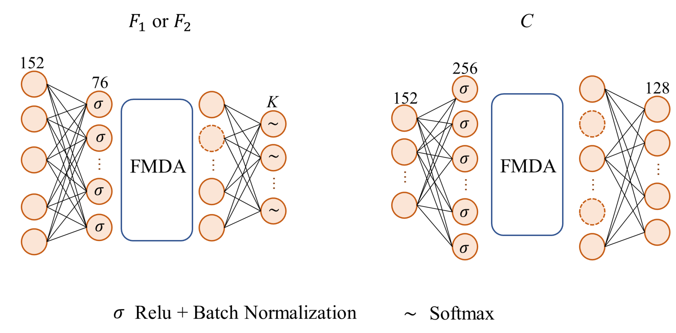
3.3. Feature Masking Data Augmentation

To assist contrastive learning tasks and improve model generalization, we propose an FMDA method based on a random feature masking technique to generate diverse training data. The masked features contain less information compared to the complete features. Therefore, the network needs to continuously improve its feature extraction ability. Compared to using complete features, leveraging masked features can encourage the network to work harder to enhance its discriminative feature extraction capabilities.

We apply FMDA on the features of the second layer (hidden layer) of the networks $F1$, $F2$ and C. Taking the network C as an example, let ${\mathit{d}}^{\left(1\right)}=(d_1^{\left(1\right)},\dots ,d_{{\mathcal{S}}_2}^{\left(1\right)})$ be a vector consisting of Bernoulli [47] variables $d_i$. ${\mathcal{S}}_2$ is the output dimension of the hidden layer of C. Given a probability function $P(d_i^{\left(1\right)}=0)=\mathsf{\rho }$, we use the following formula to represent the output of the hidden layer:

$$\begin{array}{cc}\hfill o_i^{2\left(1\right)}& =d_i^{\left(1\right)}Relu\left(\sum _{s=1}^{{\mathcal{S}}_1}{w}_{si}^1{o}_s^1+b^1\right)\hfill \\ & =\left\{\begin{array}{c}\hfill Relu\left({\displaystyle \sum _{s=1}^{{\mathcal{S}}_1}}{w}_{si}^1{o}_s^1+b^1\right)if{d}_i^{\left(1\right)}=1\hfill \\ \hfill 0if{d}_i^{\left(1\right)}=0\hfill \end{array}\right..\hfill \end{array}$$

(10)

where $w_{si}^1$ represents the connection weight between the s-th neuron in the input layer (first layer) and the i-th neuron in the hidden layer (second layer), while $o_s^1$ denotes the output of the s-th neuron in the input layer.

Because the contrastive losses use cosine distance, which is calculated based on the $L2$ norm to measure the distance between features, we introduce an $L2$-NP method. This method preserves the $L2$ norm (squared sum) of activation vectors before and after feature masking. $L2$-NP can effectively ensure that the $L2$ norm expectation of features remains consistent. ${\mathit{o}}^{2\left(1\right)}=(o_1^{2\left(1\right)},\dots ,o_{{\mathcal{S}}_2}^{2\left(1\right)})$ is the hidden feature of C with the augmentation $T_1$. To pursue an adaptive $L2$ norm, we scale the output by ${\displaystyle \frac{1}{\sqrt{1-\mathsf{\rho }}}}$ to obtain

$${\hat{o}}_i^{2\left(1\right)}={\displaystyle \frac{1}{\sqrt{1-\mathsf{\rho }}}}·o_i^{2\left(1\right)},$$

(11)

during evaluation, which satisfies

$$\begin{array}{cc}\hfill \mathbb{E}[{|{\hat{o}}_i^{2\left(1\right)}|}^2]& =\mathbb{E}[{|d_i^{\left(1\right)}{\displaystyle \frac{1}{\sqrt{1-\mathsf{\rho }}}}{o}_i^{2\left(1\right)}|}^2]\hfill \\ \hfill & ={\displaystyle \frac{1}{1-\mathsf{\rho }}}\mathbb{E}[{\left(d_i^{\left(1\right)}\right)}^2]\mathbb{E}[{|o_i^{2\left(1\right)}|}^2]\hfill \\ & =\mathbb{E}[{|o_i^{2\left(1\right)}|}^2].\hfill \end{array}$$

(12)

The output of network C is ${\mathit{o}}^{3\left(1\right)}=(o_1^{3\left(1\right)},\dots ,o_{{\mathcal{S}}_3}^{3\left(1\right)})$, where

$$o_j^{3\left(1\right)}=Relu\left(\sum _{s=1}^{{\mathcal{S}}_2}{w}_{sj}^2{\widehat{o}}_s^{2\left(1\right)}+b^2\right).$$

(13)

By generating another vector ${\mathit{d}}^{\left(2\right)}$, we can obtain a second data augmentation output ${\mathit{o}}^{3\left(2\right)}=(o_1^{3\left(2\right)},\dots ,o_{{\mathcal{S}}_3}^{3\left(2\right)})$. The schematic diagram of the FMDA method is shown in Figure 4.

This data augmentation method does not require any operations on the input image itself, and during data augmentation implementation, the entire algorithm incurs very small additional storage.

3.4. Training Steps

MTLDA combines DDML and bi-classifier adversarial training to enhance the discriminability of target domain features during domain alignment. A three-stage training approach is employed in MTLDA. In the first stage, the CE loss function is used to train the feature generator and bi-classifier, enabling the model to correctly classify source domain samples. In addition, the DDML loss function is used to improve the target domain feature discriminability. In the second stage, we train the bi-classifier to maximize classifier discrepancy, detecting target domain samples that are not supported by the source domain. To preserve feature discriminability in the target domain, the DDML loss is also employed in this stage. In the third stage, we train the feature generator to minimize classifier discrepancy on the target domain, thereby enhancing the domain-invariance of the features.

Data augmentation can generate diverse forms of target domain samples, thereby improving the model’s generalization ability [48]. Additionally, in the UDA tasks, since target domain data lacks labels, the labeled source domain data may dominate the training process. Data augmentation can mitigate the risk of overfitting by expanding the diversity of the source domain dataset. Therefore, we not only use the proposed FMDA method in DDML to assist contrastive learning but also employ FMDA during domain alignment to more effectively extract domain-invariant features. For convenience, we represent the loss functions used in the three training stages with the following three equations:

$${\mathcal{L}}_{ce}\left({\stackrel{\sim }{\mathbf{X}}}^s,{\stackrel{\sim }{\mathbf{Y}}}^s\right)+\alpha ·{\mathcal{L}}_{ddml}({\stackrel{\sim }{\mathbf{X}}}^s,{\stackrel{\sim }{\mathbf{Y}}}^s,{\stackrel{\sim }{\mathbf{X}}}^t),$$

(14)

$${\mathcal{L}}_{ce}\left({\stackrel{\sim }{\mathbf{X}}}^s,{\stackrel{\sim }{\mathbf{Y}}}^s\right)+\alpha ·{\mathcal{L}}_{ddml}({\stackrel{\sim }{\mathbf{X}}}^s,{\stackrel{\sim }{\mathbf{Y}}}^s,{\stackrel{\sim }{\mathbf{X}}}^t)-{\mathcal{L}}_d\left({\stackrel{\sim }{\mathbf{X}}}^t\right),$$

(15)

and

$${\mathcal{L}}_d\left({\stackrel{\sim }{\mathbf{X}}}^t\right).$$

(16)

The training process can be summarized as Algorithm 1. During testing, the output of $F1$ is used as the classification result for the sample.

Algorithm 1 Training process of MTLDA

Input: Target domain data: ${\mathbf{X}}^t$, labels and source domain data: (${\mathbf{X}}^s$, ${\mathbf{Y}}^s$), batch size B, hyperparameter: $\alpha$ and ${\tau }_c$, the number of epochs: $NU\mathrm{M\_}EPOCH$, the number of iterations for the training of G to minimize the classifier discrepancy: $NU\mathrm{M\_}ITR$. Output: ${\mathit{\theta }}_G$, ${\mathit{\theta }}_{F1}$ and ${\mathit{\theta }}_{F2}$. 1:  for each $i\in [1,NU\mathrm{M\_}EPOCH]$ do 2:      random sample B source samples and B target samples. 3:      apply FMDA to the sampled data twice to obtain augmented batches. 4:      update ${\mathit{\theta }}_G$, ${\mathit{\theta }}_{F1}$, ${\mathit{\theta }}_{F2}$, ${\mathit{\theta }}_C$ through minimizing the loss function presented in Equation (14). 5:      update ${\mathit{\theta }}_{F1}$, ${\mathit{\theta }}_{F2}$ and ${\mathit{\theta }}_C$ through minimizing the loss function presented in Equation (15). 6:      for each $j\in [1,NU\mathrm{M\_}ITR]$ do 7:          update ${\mathit{\theta }}_G$ through minimizing the loss function presented in Equation (16). 8:      end for 9:  end for

4. Results

4.1. Dataset Description

Three mainstream hyperspectral classification datasets: Houston, Pavia and HyRANK are used to validate the effectiveness of our method.

4.1.1. Houston Dataset

The Houston datasets comprise two sub-datasets: Houston 2013 (source domain) and Houston 2018 (target domain), acquired at the University of Houston campus and its surrounding metropolitan area. For the purpose of analysis, an overlapping area of 209 × 955 pixels was selected from the Houston 2013 dataset, encompassing 48 spectral bands corresponding to the Houston 2018 dataset. Figure 5 illustrates the ground-truth maps and pseudo-color images pertaining to the Houston dataset.

4.1.2. Pavia Dataset

The two sub-datasets used in the Pavia task were taken at Pavia University (PaviaU, source domain) and Pavia Center (PaviaC, target domain), respectively, by the ROSIS sensor. There are 103 spectral bands and dimensions of 610 × 315 pixels in the PaviaU and 102 spectral bands and dimensions of 1096 × 715 pixels in the PaviaC. The last band of PaviaU is not available in PaviaC. For the convenience of analysis, we remove this band. Figure 6 illustrates the ground-truth maps and pseudo-color images pertaining to the Pavia dataset.

4.1.3. HyRANK Dataset

The HyRANK dataset [49] is an important satellite resource captured in two regions: Dioni (source domain) and Loukia (target domain). The HSIs in HyRANK were acquired by the Hyperion sensor, and each Hyperion hyperspectral datacube consisted of 176 remaining bands. These two HSIs comprise 250 × 1376 pixels and 249 × 945 pixels, respectively. These scenes include identical 12 land cover classes. The comparison between the source and target domains is shown in Figure 7.

4.2. Experimental Setup

Next, we introduce the experimental settings of the seven other algorithms mentioned in the comparative experiment, including Deep Adaptation Network (DAN) [16], Domain Adversarial Neural Network (DANN) [20], ED-DMM-UDA [21], Classwise Distribution Adaptation (CDA) [22], TAADA [23], SCLUDA [18] and MSDA [25].

We select $180\times K$ samples from the source domain dataset for training to ensure balanced class labels. If any class has fewer than 180 samples, we utilize all available samples from that class. For DAN, we use the ResNet50 network as the feature extractor, incorporating five unique Gaussian kernels. The batch size is 32, with a training iteration count of 1000. Stochastic Gradient Descent (SGD) is adopted as the gradient optimization algorithm, equipped with a momentum of 0.9 and a weight decay of 0.0005. For DANN [20], we employ a feature extractor utilizing the ResNet18 network, coupled with a discriminator comprising three fully connected layers. The learning rate is set to 0.01, with a batch size of 32. The training encompasses 1000 epochs. ED-DMM-UDA [21] involves source domain training over 1000 epochs, while target domain training is restricted to 20 epochs. CDA [22] is executed with a batch size of 32. The learning rates for the respective tasks are established at 0.001, 0.05, and 0.05. The parameters $lambd{a}_1$ and $lambd{a}_2$ are adjusted to ratios of 10:1, 1:1, and 1:1 for the varying tasks. TAADA [23] adheres to the configuration as outlined in the original paper. For SCLUDA [18], we preserve the parameters for the Houston dataset in accordance with the original publication. However, for the HyRANK dataset, we adjust the values of $\alpha$, $\beta$, and $\gamma$ to 0.01, 0.01, and 0.03, respectively. Lastly, for the MSDA method [25], we adopt the settings directly from the original paper. In our experiments, we set the ${\tau }_c$ to 0.5, the ${\mathcal{S}}_2$ to 256, and the ${\mathcal{S}}_3$ to 128. For the Houston task, the patch size is $7\times 7\times 48$. We set the hyperparameter $\alpha$ to 0.02, $NU\mathrm{M\_}EPOCH$ to 50, the learning rate ($lr$) to 0.02, and the batch size (B) to 64. For the Pavia task, the patch size is $9\times 9\times 102$. We set $\alpha$ to 0.1, $NU\mathrm{M\_}EPOCH$ to 60, $lr$ to 0.008, and B to 32. For the HyRANK task, the patch size is $3\times 3\times 176$. We set $\alpha$ to 0.03, the epochs $NU\mathrm{M\_}EPOCH$ to 25, $lr$ to 0.004, and B to 32. For training, we follow SDAT [50], which utilizes CDAN [51] with MCC [52]. The temperature settings in the MCC loss are, respectively, 18, 4, and 8 for the Houston, Pavia, and HyRANK tasks. To evaluate the experimental results, we primarily utilize three metrics: Overall Accuracy (OA), Average Accuracy (AA), and the Kappa coefficient ($\mathsf{\kappa }$).

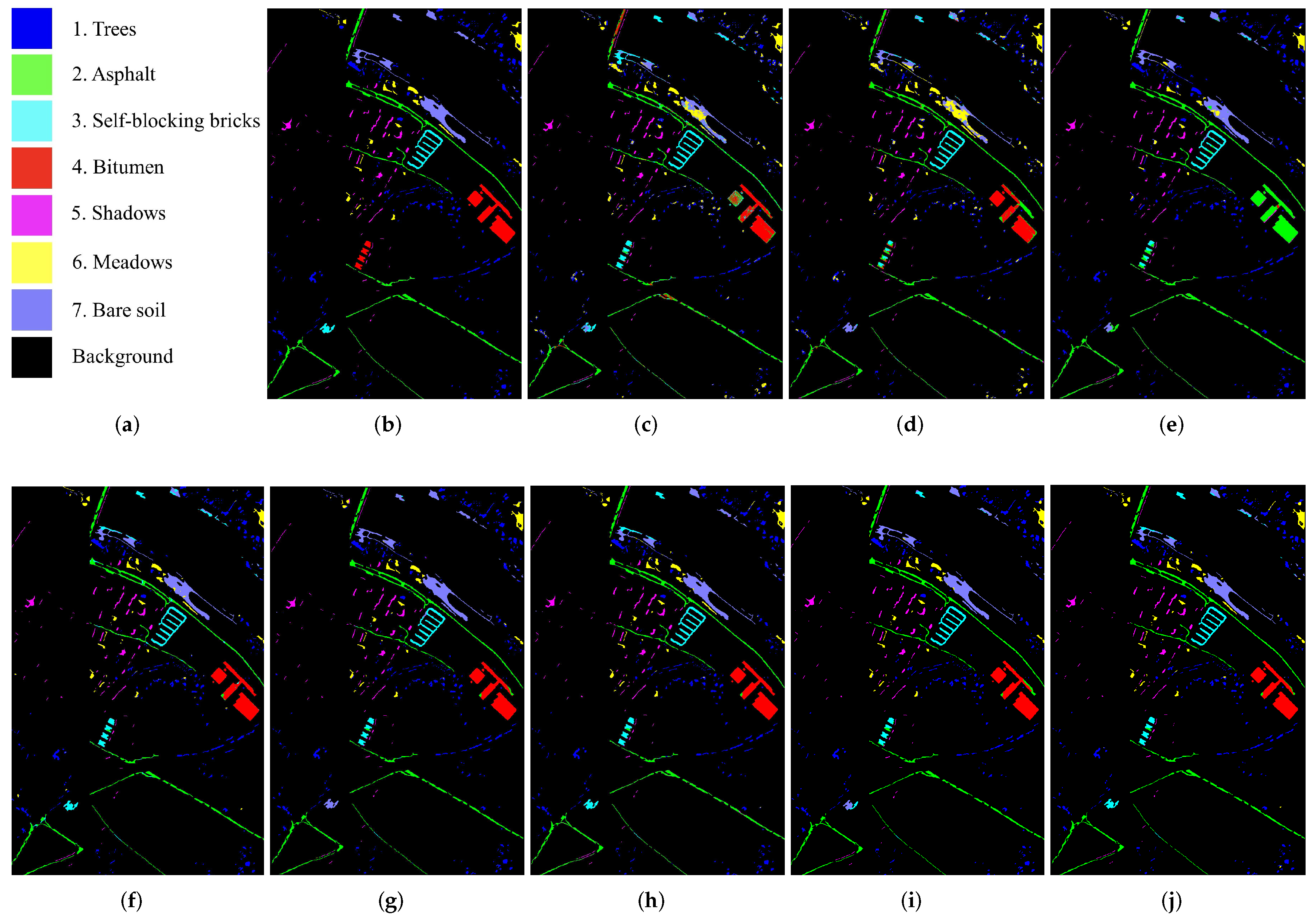
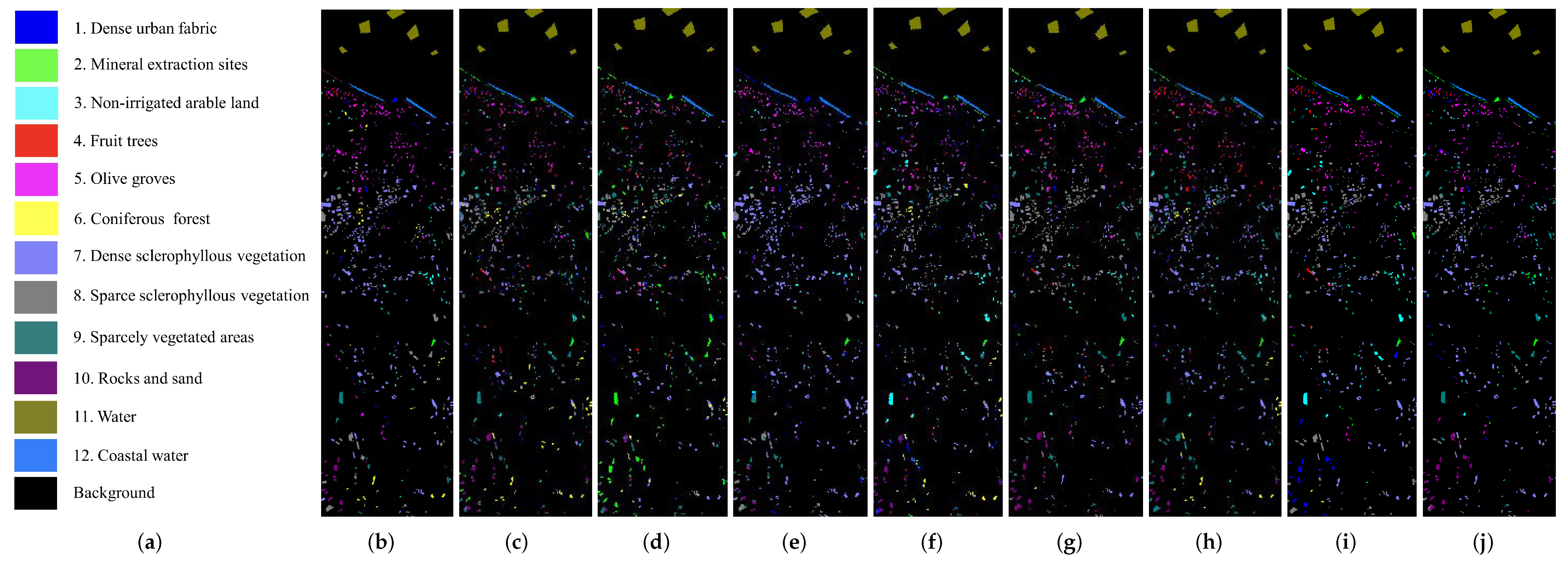
4.3. Comparison and Analysis

Table 1. Comparison of classification accuracy (values ± standard deviation) across different methods in the Houston task.

Class	DAN (2015)	DANN (2017)	ED-DMM-UDA (2020)	CDA (2021)	TAADA (2022)	SCLUDA (2023)	MSDA (2024)	Ours
1	89.08	79.71	68.14	95.08	94.29	81.32	81.66	8.26
2	56.09	73.26	85.45	51.96	53.03	71.58	52.95	93.62
3	79.55	70.91	57.86	62.52	53.13	62.67	57.81	58.77
4	89.55	98.18	79.55	95.45	97.27	90.00	85.00	76.36
5	69.04	69.61	97.77	70.35	80.42	85.11	91.01	77.56
6	50.61	55.72	56.62	82.74	76.61	80.53	76.79	89.28
7	66.66	60.81	75.97	26.26	75.64	49.13	74.83	73.73
OA (%)	57.39	60.75	66.09	71.18	73.95	75.50	74.94	82.99
	±1.19	±5.03	±1.83	±1.31	±2.65	±1.77	±2.58	±1.11
AA (%)	71.51	72.6	74.48	69.20	75.77	74.32	74.29	68.23
	±1.09	±2.05	±1.66	±3.16	±2.31	±4.93	±7.08	±3.27
$\mathsf{\kappa }\times 100$	43.25	45.85	53.10	51.85	60.29	61.00	61.59	72.04
	±1.16	±4.45	±2.18	±3.23	±3.35	±3.38	±4.95	±1.65

Bolded values indicate the optimal result in each row.

presents the results of comparison experiments of various UDA methods for HSI classification in the Houston task. MTLDA achieves the highest OA (82.99%) and $\mathsf{\kappa }$ (72.04%), demonstrating its effectiveness in cross-scene HSI classification and it surpasses all comparison methods that use pseudo labels as target domain guidance signals. This result suggests that the combination of inductive transfer mechanisms and representation learning methods can help improve the discriminability of target domain features in domain adaptation, even without pseudo-label guidance signals. Figure 8 displays the classification maps of different comparative algorithms.

From the results of individual categories, MTLDA achieved the highest classification accuracy in both “non-residential buildings” and “stressed grass” categories, but the lowest classification accuracy in the category of “healthy grass”. It can be seen from Figure 8 that the MTLDA’s incorrect classification of “healthy grass” as “stress grass” leads to this result. This may be caused by the FMDA algorithm, because HSIs reflect the material characteristics of objects. Therefore, the features of hyperspectral data with similar materials are also extremely similar. During the training process, FMDA randomly masks half of the feature information for each training datapoint. This operation is likely to mask the parts of the features that can distinguish similar materials, resulting in class confusion in the classification of similar classes. For other objects with similar materials in the Houston task, such as “Residential buildings” and “Non-residential buildings”, the classification accuracy of our method reaches 77.56% and 89.28%, respectively. MTLDA can effectively differentiate between these two similar categories. These results show that the bad influence of FMDA is limited. From Figure 8, we can also visually see that MTLDA is more accurate for the classification of two types of buildings.

The comparative experimental results of various algorithms of the Pavia task are presented in

Table 2. Comparison of classification accuracy (values ± standard deviation) across different methods in the Pavia task.

Class	DAN (2015)	DANN (2017)	ED-DMM-UDA (2020)	CDA (2021)	TAADA (2022)	SCLUDA (2023)	MSDA (2024)	Ours
1	72.79	84.49	98.15	92.02	91.50	95.97	93.66	95.36
2	79.37	90.51	94.12	77.63	98.72	98.44	99.06	99.44
3	87.50	75.86	64.02	86.90	57.07	98.03	64.26	96.53
4	67.76	71.28	0.72	78.17	69.94	85.7	78.30	83.88
5	98.75	99.58	96.61	99.94	97.50	98.42	99.78	99.99
6	80.22	69.52	68.29	61.81	92.94	96.68	93.79	96.10
7	58.37	62.67	64.79	71.60	95.46	78.13	96.59	89.04
OA (%)	74.47	79.14	68.80	80.51	88.07	91.91	91.03	93.61
	±2.07	±2.68	±2.58	±1.02	±5.97	±0.44	±1.82	±0.22
AA (%)	77.82	79.13	69.53	81.15	86.16	92.82	89.35	94.33
	±1.90	±1.96	±2.41	±1.81	±6.71	±0.60	±3.25	±0.38
$\mathsf{\kappa }\times 100$	69.79	75.02	62.47	76.68	85.72	92.36	89.19	92.34
	±2.43	±3.12	±3.16	±1.22	±7.04	±0.40	±2.21	±0.26

Bolded values indicate the optimal result in each row.

. Figure 9 provides a visual comparison of the classification maps. MTLDA achieves the highest OA (93.61%), AA (94.33%) and Kappa (92.34%), indicating its superiority. SCLUDA and MSDA also exhibit strong performances, with OA reaching 91.91% and 91.03%, respectively. SCLUDA and MSDA both use pseudo-labels during training, which suggests that pseudo-labels can improve the discriminability of features to some extent. The OA, AA, and Kappa values of the TAADA method are second only to SCLUDA, MSDA and MTLDA. These four methods adopt a spatial–spectral dual-branch network structure as the generator, which demonstrates the superior performance of this network structure. For the classification performance of each individual category, ED-DMM-UDA, MSDA, and SCLUDA have achieved the highest classification accuracy in one or more classes. However, the AA and OA of these methods are lower than MTLDA. From Table 2, it can be seen that these methods all have a relatively low classification accuracy in a certain category. For example, the classification accuracy of ED-DMM-UDA in class ‘4’ and TAADA in class ‘3’ are only 0.72% and 57.07%, respectively. The classification accuracy of MTLDA exceeds 80% in each class. This shows that compared to the comparison method, MTLDA can extract more discriminative features. As can be seen from Figure 9, MTLDA is accurate in distinguishing “Trees”, “Shadow” and “Meadow”. There is almost no class confusion in the easily confused categories of “Trees” and “Meadows”, “Shadows” and “Asphalt”.

Table 3. Comparison of classification accuracy (values ± standard deviation) across different methods in the HyRANK task.

Class	DAN (2015)	DANN (2017)	ED-DMM-UDA (2020)	CDA (2021)	TAADA (2022)	SCLUDA (2023)	MSDA (2024)	Ours
1	33.98	19.81	69.81	30.05	45.68	36.94	28.40	34.47
2	100	96.30	91.48	85.93	100	71.85	89.07	97.59
3	57.09	31.48	59.65	77.84	76.95	56.83	85.12	81.46
4	74.81	69.75	40.51	28.35	65.44	96.71	61.90	32.53
5	35.98	19.79	47.53	58.84	71.62	12.97	77.38	80.36
6	31.35	26.28	12.61	42.77	5.73	54.83	2.25	0.73
7	49.78	43.05	78.19	50.02	41.64	78.57	46.00	63.53
8	31.79	30.47	49.25	22.64	50.7	27.69	60.42	52.13
9	61.88	31.68	64.26	23.31	26.74	85.16	30.05	57.37
10	54.64	31.37	54.97	63.75	20.68	50.42	26.78	58.98
11	99.25	89.39	70.00	60.02	100	100	100	100
12	76.94	95.11	68.08	99.98	100	100	100	100
OA (%)	52.34	43.96	61.37	48.14	56.25	60.08	60.52	66.23
	±1.51	±4.49	±9.04	±0.06	±2.96	±2.47	±2.90	±1.72
AA (%)	59.96	48.71	58.86	53.63	58.77	64.33	58.95	63.26
	±1.58	±3.49	±3.40	±4.56	±3.23	±5.10	±2.74	±3.21
$\mathsf{\kappa }\times 100$	43.23	34.91	54.33	40.89	48.67	53.65	53.15	59.84
	±2.28	±4.48	±3.40	±6.57	±3.12	±2.69	±3.35	±1.99

Bolded values indicate the optimal result in each row.

succinctly summarizes the experimental outcomes in the HyRANK dataset. Figure 10 presents a visual comparison of classification maps, providing an illustrative comparison of their performance. MTLDA achieves the highest accuracy on 3 out of 12 classes (from 80.36% to 100%), demonstrating its strong performance on the classification of a variety of land cover types. SCLUDA outperforms other methods on classes ‘3’, ‘5’, ‘6’, ‘8’, ‘10’ and ‘11’ (from 54.83% to 100%), while its overall OA and $\mathsf{\kappa }$ scores are inferior to the MTLDA method. MTLDA achieves the highest OA (66.23%) and the highest $\mathsf{\kappa }$ (59.84%). This indicates that MTLDA has achieved good performance in both overall classification and classification for each category. As can be seen from Table 3, all algorithms except DAN have a classification accuracy of less than 30% in one or more classes. The classification accuracies of DAN in classes ‘6’ and ‘8’ are merely 31.35% and 31.79%, respectively. This may be due to the fact that the HyRANK dataset has many categories related to vegetation. These categories are very similar in terms of material characteristics. Due to the lack of label guidance, domain adaptation classification methods are prone to confusion for these categories. This is also one of the difficulties that future UDA methods for HSI classification need to overcome.

4.4. Ablation Study Results

Two sets of ablation experiments were performed to assess the impact of TCL and SCL on the results. The OA outcomes are shown in

Table 4. Ablation study for DDML.

No.	SCL	TCL	Houston	Pavia	HyRANK
1	✘	✘	77.54	92.15	62.67
			±4.51	±1.37	±3.12
2	✘	✔	70.04	93.38	65.64
			±3.39	±0.73	±0.71
3	✔	✘	75.88	91.95	63.19
			±3.82	±1.26	±3.07
4	✔	✔	82.99	93.61	66.23
			±1.11	±0.22	±1.72

Bolded values indicate the optimal result in each column.

. The inclusion of both TCL and SCL in the model results in the highest OA values of 82.99%, 93.61%, and 66.23%. However, using TCL or SCL alone in the Houston task decreases the model’s classification performance, with decreases from 77.54% to 70.04% and from 77.54% to 75.88%, respectively. On the contrary, incorporating contrastive learning can help improve model performance in the HyRANK task (from 62.67% to 65.65% and from 62.67% to 63.19%). The reasons for this situation may be as follows.

Optimizing only SCL loss can enhance the discriminability of source features, not target features. Optimizing only the TCL loss can improve the discriminability of the target domain features. But TCL is a unsupervised representation learning method, so it cannot learn the information from the label to improve the accuracy of classification. When optimizing one loss function alone, the model cannot simultaneously consider the discriminability and classification knowledge. Focusing only on the discriminability of target features and ignoring classification information or focusing only on the discriminability of the source features may improve the performance of the model, but it may also cause the optimization direction of the network weights to deviate, resulting in a decrease in classification performance.

To demonstrate the effectiveness of SCL and TCL in enhancing feature separability and discriminability, we utilized t-SNE [53] to visualize the target output of the feature generator. The figures in Figure 11 can be divided into three groups: Figure 11a,d, Figure 11b,e and Figure 11c,f. The source domain training data used for the two images within each group are identical. As shown in Figure 11, the target domain features learned with contrastive learning exhibit greater intra-class compactness, and the features of each class are clustered together. Without employing contrastive learning, the learned features exhibit a relatively dispersed distribution. Some features belonging to the same category have not been clustered together, as is the case for classes ’2’ and ’3’ in Figure 11d–f.

To verify the effectiveness of FMDA, three extra comparative experiments were conducted on data augmentation, whose results are presented in

Table 5. Comparison of different data augmentation methods.

Datasets	Metrics	FMDA (Ours)	HF	VF	RPE
Houston	OA (%)	82.99	78.97	78.27	74.17
		±1.11	±3.19	±1.89	±4.54
	AA (%)	68.23	71.50	67.94	61.52
		±3.27	±3.52	±6.70	±5.12
	$\mathsf{\kappa }\times 100$	72.04	66.39	64.50	54.88
		±1.65	±7.48	±3.28	±4.48
	training time	180.31	278.36	288.12	320.54
Pavia	OA (%)	93.61	92.21	91.71	90.88
		±0.22	±1.57	± 1.71	±1.72
	AA (%)	94.33	92.96	92.37	92.03
		±0.38	±1.69	±2.16	±1.40
	$\mathsf{\kappa }\times 100$	92.34	90.67	90.08	89.10
		±0.26	±1.86	±2.04	±2.03
	training time	621.33	865.09	866.37	903.51
HyRANK	OA (%)	66.23	62.19	62.76	63.93
		±1.72	±3.13	±3.23	±1.82
	AA (%)	63.26	59.84	60.55	64.78
		±3.21	±4.12	±4.40	±1.14
	$\mathsf{\kappa }\times 100$	59.84	55.30	55.94	57.36
		±1.99	±3.54	±2.63	±2.01
	training time	135.18	180.31	184.88	215.76

Bolded values indicate the optimal result in each row.

. We employed three additional HSI augmentation methods mentioned in paper [36]: Horizontal Flipping (HF), Vertical Flipping (VF) and Random Pixel Erasing (RPE) for comparison. Compared to the other three input-based data augmentation techniques, FMDA performed better on the vast majority of metrics. This indicates that the FMDA method can effectively enhance classification accuracy. In the Houston task and HyRANK task, AA achieved by the model using FMDA (68.23% and 63.26%) was lower than that achieved using HF (71.50%) and RPE (64.78%), respectively. This situation is consistent with our subsequent analysis that FMDA may mask the distinguishable part of the features, resulting in slight class confusion. Additionally, we designed an ablation experiment to verify the contribution of $L2$-NP to cross-scene HSI classification accuracy. From

Table 6. Ablation study of $L2$-NP.

Methods	Houston			Pavia			HyRANK
	OA (%)	AA (%)	$\mathsf{\kappa }\times \mathbf{100}$	OA (%)	AA (%)	$\mathsf{\kappa }\times \mathbf{100}$	OA (%)	AA (%)	$\mathsf{\kappa }\times \mathbf{100}$
MTLDA* (w/o $L2$-NP)	81.32	67.92	70.29	93.51	93.97	91.85	64.57	59.46	58.62
	±2.45	±1.61	±3.71	±0.47	±1.03	±0.92	±2.36	±3.89	±2.65
MTLDA	82.99	68.23	72.04	93.61	94.33	92.34	66.23	63.26	59.84
	±1.11	±3.27	±1.65	±0.22	±0.38	±0.26	±1.72	±3.21	±1.99

^* signifies that L2-NP is removed from the MTLDA method.

, it can be seen that after adding $L2$-NP to the proposed model, OA shows different increases in the three tasks, rising by 1.67%, 0.1%, and 1.66%, respectively. AA and $\mathsf{\kappa }$ also show increases in all three tasks. This suggests that adding $L2$-NP is beneficial for enhancing the model’s cross-scene HSI classification performance.

4.5. Comparison and Analysis of Data Augmentation Methods During Domain Alignment

Compared to the bi-classifier adversarial UDA baseline for HSI classification, MTLDA additionally employs data augmentation methods during the domain alignment process. To investigate the contribution of data augmentation methods during the domain alignment, we designed five groups of comparative experiments to obtain the quantitative results and training duration when using them. The experimental results are shown in

Table 7. Comparison of experimental results of data augmentation methods during domain alignment.

Datasets	Metrics	Baseline	FMDA + Baseline	HF + Baseline	VF + Baseline	RPE + Baseline
Houston	OA (%)	74.07	77.45	77.66	76.53	63.20
		±3.59	±4.51	±1.64	±2.51	±7.07
	AA (%)	65.66	68.42	68.00	66.98	41.94
		±4.89	±5.04	±2.98	±4.99	±8.51
	$\mathsf{\kappa }\times 100$	62.71	66.91	66.07	64.66	38.15
		±4.96	±6.12	±2.29	±5.76	±9.05
	training time	149.47	172.73	298.70	299.01	310.29
Pavia	OA (%)	91.01	92.15	91.78	91.03	72.32
		±0.32	±1.37	±1.68	±1.64	±5.03
	AA (%)	92.13	93.35	92.46	91.87	73.11
		±0.87	±1.22	±1.81	±1.86	±4.54
	$\mathsf{\kappa }\times 100$	89.94	91.08	90.16	89.28	66.81
		±1.39	±1.17	±1.99	±1.95	±5.91
	training time	456.12	473.99	814.47	821.97	856.61
HyRANK	OA (%)	60.71	62.67	59.27	60.06	58.76
		±2.51	±3.12	±4.59	±3.39	±3.00
	AA (%)	53.26	57.85	55.48	55.86	57.35
		±2.58	±3.82	±4.29	±3.88	±6.61
	$\mathsf{\kappa }\times 100$	55.04	56.00	51.75	52.67	51.13
		±1.85	±3.69	±5.26	±3.88	±3.75
	training time	134.62	138.63	176.99	178.87	175.22

Bolded values indicate the optimal result in each row.

. The baseline in the table refers to the model that uses only bi-classifier adversarial training. Based on the baseline, we performed four sets of experiments, where each set introduces one type of data augmentation. We generate two augmented samples for each training sample and use these augmented samples for domain alignment. The FMDA method achieved the best performance in most tasks, with an OA of 92.15% in the Pavia task and an OA of 62.67% in the HyRANK task. In the Houston task, its OA was only 0.21% lower than that of the HF method. This indicates the effectiveness of FMDA during the domain alignment process. Furthermore, all methods using data augmentation outperformed the baseline method, indicating that employing data augmentation during alignment can improve cross-scene HSI classification performance. In terms of training duration, the method incorporating FMDA increases the training time compared to the baseline by 23.26 s, 17.87 s, and 4.01 s on the three tasks, respectively. Nonetheless, its OA showed noticeable improvements, with increases of 3.38%, 1.14%, and 1.96%, respectively. Additionally, among all models that incorporate data augmentation, FMDA demonstrated the shortest training duration. This may be because, for a given input data, other methods require per-sample forward propagation for each augmented sample, while FMDA performs data augmentation on the classifier’s hidden-layer features, thus requiring only a single forward pass from input to hidden layers.

4.6. Parameter Analysis

In our algorithm, the important hyperparameters include patch size ($ps$), success probability for Bernoulli variables ($\mathsf{\rho }$) in the FMDA, temperature (${\tau }_c$) in the contrastive learning, a coefficient ($\alpha$) to balance with the contrastive learning loss and the adversarial loss, and the dim of contrastive features (${\mathcal{S}}_3$). The ranges for the hyperparameters are as follows: $\mathsf{\rho }$ is in the range [0.1, 0.2, 0.3, 0.4, 0.5, 0.6, 0.7, 0.8, 0.9]; $ps$ is in the range [3, 5, 7, 9]; ${\tau }_c$ is in the range [0.1, 0.2, 0.3, 0.4, 0.45, 0.5, 0.55, 0.6, 0.7, 0.8, 0.9, 1.0]; $\alpha$ is in the range [0.01, 0.02, 0.03, 0.04, 0.05, 0.06, 0.07, 0.08, 0.09, 0.1]; and ${\mathcal{S}}_3$ is in the range [32, 64, 96, 128, 196, 256, 512]. Figure 12 shows the comparison of OA among the three tasks when different parameter settings are used. For a $ps$ parameter, a larger $ps$ can provide more spatial information. In the Pavia task, the source and target domains have similar spatial environments, so larger $ps$ can achieve better performance. In contrast, for the HyRANK task, the spatial similarity between the source and target domains is lower, making it advisable to choose a smaller $ps$. We set the $ps$ to 7, 3, and 9 for the Houston, Pavia, and HyRANK tasks, respectively. $\mathsf{\rho }$ is the success probability of the Bernoulli variable in the FMDA method. As can be seen from Figure 12b, the three tasks perform best when $\mathsf{\rho }$ is 0.5, so we set it to 0.5 for these three tasks. For the hyperparameter ${\tau }_c$, it is the temperature coefficient used in contrastive learning. As shown in Figure 12c, when ${\tau }_c>0.1$, the performance of the three tasks is not very sensitive to its value. Following the common practice, we set ${\tau }_c$ to 0.5 for these three tasks. We set ${\mathcal{S}}_3$ to 128 for the three tasks, as this dimensionality balances representational capacity and computational efficiency, ultimately benefiting model performance. $\alpha$ is the coefficient that balances the adversarial loss and the dual-domain contrastive learning loss. A larger $\alpha$ indicates that the model is more influenced by the contrastive learning loss. As shown in Figure 12e, the Houston and HyRANK tasks are relatively sensitive to $\alpha$, while Pavia exhibits relatively stable performance. We set $\alpha$ to 0.02, 0.03, and 0.1 for the Houston, Pavia, and HyRANK tasks, respectively, for the best performances. During the hyperparameter tuning process, we first determine the value of $ps$, then establish $\mathsf{\rho }$, followed by sequentially determining the two hyperparameters related to contrastive learning: ${\tau }_c$ and ${\mathcal{S}}_3$. Finally, we establish the coefficient $\alpha$.

4.7. Computational Complexity

The comparison of computational complexity is shown in

Table 8. Comparison of training time (seconds), testing time (seconds), FLOPs, and count of parameters across different methods.

Datasets		DAN (2015)	DANN (2017)	ED-DMM-UDA (2020)	CDA (2021)	TAADA (2022)	SCLUDA (2023)	MSDA (2024)	Ours
Houston	Training time	664.75	28.59	941.54	207.86	205.63	135.27	192.34	180.31
	Testting time	5.33	5.89	14.82	0.68	2.67	4.46	4.16	3.68
	FLOPs	4606599	15873800	6555402	19648507	7678089	7678089	15489249	15610464
	#params	25701743	13159880	170274	76757	577640	572241	1120456	585207
Pavia	Training time	648.98	31.81	305.95	201.21	283.82	331.25	433.72	621.33
	Testting time	4.61	5.77	13.72	0.47	3.81	4.44	3.76	5.60
	FLOPs	15017863	23784392	11686202	23104507	50180201	80408762	50170234	50242088
	#params	25871087	13329224	181074	90257	661880	676017	1393035	690443
HyRANK	Training time	459.12	38.43	1194.21	383.59	211.59	327.65	344.23	135.18
	Testting time	1.24	1.99	10.01	0.06	0.71	0.87	0.75	0.68
	FLOPs	3655052	15227149	1465802	28160512	29503089	80408762	9396179	9480696
	#params	26105716	13563853	195874	110012	811028	876017	1609392	837449

. The deep learning framework is open-source PyTorch 1.13. The computational complexity experiments were conducted on a computer equipped with an NVIDIA GeForce RTX 3090 GPU and an Intel Xeon Gold 6226R CPU. Table 8 presents a detailed comparison of computational complexities, encompassing training duration, testing duration, floating-point operations (FLOPs), and parameter count.

5. Discussion

We compared the cross-domain HSI classification performance of MTLDA with seven other renowned UDA methods using three mainstream datasets. These methods encompass various domain alignment approaches and different strategies to enhance the discriminability of target domain features, and MTLDA achieved the best performance among all the methods. Overall, adversarial-based domain alignment methods slightly outperformed discrepancy-based domain alignment methods. Among all adversarial-based methods, the superior performances of domain alignment approaches based on bi-classifier, such as TAADA, MSDA, indicate their suitability for cross-scene HSI classification. From the visualization results, it is evident that the proposed strategy combining multi-task learning with representation learning effectively enhances the inter-class separability and intra-class compactness of target domain features, which is highly beneficial for improving the accuracy of cross-domain classification. As can be seen from Table 5, the proposed FMDA method not only saves training time compared to previous data augmentation methods but also achieves optimal results across all three datasets. In addition, almost all comparison methods perform the worst on the HyRANK task, achieving an average OA of 56.11%, while they perform the best on the Pavia task, reaching an average OA of 83.44%. In the Pavia task, the source domain and target domain are captured over two locations that are very close to each other, and the capture time is the same. The relatively mild domain shift makes it easier for the model to capture domain-invariant information. In the HyRANK task, the HSIs of the source domain and target domain are captured over geographically distant areas, resulting in relatively significant inter-domain differences. Additionally, the categories in this dataset are mainly vegetation types, which have similar material characteristics, making it difficult for the model to extract spectral discriminative features. Furthermore, the spatial similarity between the source domain and target domain is not obvious, making it challenging to capture domain-invariant information from a spatial perspective, which further increases the difficulty of the task. In the Houston task, there are minor spatial differences between the source domain and target domain, and the distinguishability of category materials makes it easier for the model to extract discriminative features. In summary, when the classes in the dataset are similar or the spatial environments in the source and target domains are dissimilar, the performance of cross-scene HSI classification is generally poor. Enhancing the model’s ability to extract spectral features to distinguish between categories with similar materials or designing a new domain alignment approach that specifically aims at mitigating the large spatial domain discrepancies may improve the performance of cross-domain HSI classification.

6. Conclusions

In this article, an MTLDA method is presented that integrates multi-task learning with adversarial training to enhance the feature discriminability during domain alignment. Furthermore, SCL and TCL are utilized to construct multi-task learning, encouraging the model to transfer the source domain classification knowledge to the target domain. Finally, an FMDA method for HSI is introduced to assist contrastive learning tasks and provide more diverse training data. The experimental results indicate that our method achieved excellent performance. However, incorporating multi-task learning in MTLDA and employing data augmentation during alignment increases the training duration. In the future, optimization techniques will be explored to improve training efficiency.

References

1. Cui, Y.; Meng, F.; Fu, P.; Yang, X.; Zhang, Y.; Liu, P. Application of Hyperspectral Analysis of Chlorophyll a Concentration Inversion in Nansi Lake. Ecol. Inform. 2021, 64, 101360. [Google Scholar] [CrossRef]
2. Thangavel, K.; Spiller, D.; Sabatini, R.; Amici, S.; Sasidharan, S.T.; Fayek, H.; Marzocca, P. Autonomous Satellite Wildfire Detection Using Hyperspectral Imagery and Neural Networks: A Case Study on Australian Wildfire. Remote Sens. 2023, 15, 720. [Google Scholar] [CrossRef]
3. Lu, B.; Dao, P.D.; Liu, J.; He, Y.; Shang, J. Recent Advances of Hyperspectral Imaging Technology and Applications in Agriculture. Remote Sens. 2020, 12, 2659. [Google Scholar] [CrossRef]
4. Sabins, F.F. Remote Sensing for Mineral Exploration. Ore Geol. Rev. 1999, 14, 157–183. [Google Scholar] [CrossRef]
5. Tejasree, G.; Agilandeeswari, L. An Extensive Review of Hyperspectral Image Classification and Prediction: Techniques and Challenges. Multimed. Tools Appl. 2024, 83, 80941–81038. [Google Scholar] [CrossRef]
6. Lou, C.; Al-qaness, M.A.A.; AL-Alimi, D.; Dahou, A.; Elaziz, M.A.; Abualigah, L.; Ewees, A.A. Land Use/Land Cover (LULC) Classification Using Hyperspectral Images: A Review. Geo-Spat. Inf. Sci. 2024, 1–42. [Google Scholar] [CrossRef]
7. Guan, R.; Li, Z.; Tu, W.; Wang, J.; Liu, Y.; Li, X.; Tang, C.; Feng, R. Contrastive Multiview Subspace Clustering of Hyperspectral Images Based on Graph Convolutional Networks. IEEE Trans. Geosci. Remote Sens. 2024, 62, 5510514. [Google Scholar] [CrossRef]
8. Feng, J.; Wang, Q.; Zhang, G.; Jia, X.; Yin, J. CAT: Center Attention Transformer with Stratified Spatial–Spectral Token for Hyperspectral Image Classification. IEEE Trans. Geosci. Remote Sens. 2024, 62, 5615415. [Google Scholar] [CrossRef]
9. Sun, L.; Zhang, H.; Zheng, Y.; Wu, Z.; Ye, Z.; Zhao, H. MASSFormer: Memory-augmented Spectral-Spatial Transformer for Hyperspectral Image Classification. IEEE Trans. Geosci. Remote Sens. 2024, 62, 5516415. [Google Scholar] [CrossRef]
10. Tuia, D.; Persello, C.; Bruzzone, L. Domain Adaptation for the Classification of Remote Sensing Data: An Overview of Recent Advances. IEEE Geosci. Remote Sens. Mag. 2016, 4, 41–57. [Google Scholar] [CrossRef]
11. Wilson, G.; Cook, D.J. A Survey of Unsupervised Deep Domain Adaptation. ACM Trans. Intell. Syst. Technol. 2020, 11, 51. [Google Scholar] [CrossRef]
12. Yang, X.; Song, Z.; King, I.; Xu, Z. A Survey on Deep Semi-Supervised Learning. IEEE Trans. Knowl. Data Eng. 2023, 35, 8934–8954. [Google Scholar] [CrossRef]
13. Huang, J.; Gretton, A.; Borgwardt, K.; Schölkopf, B.; Smola, A. Correcting Sample Selection Bias by Unlabeled Data. In Proceedings of the Advances in Neural Information Processing Systems, Vancouver, BC, Canada, 4–7 December 2006; Volume 19. [Google Scholar]
14. Yaras, C.; Kassaw, K.; Huang, B.; Bradbury, K.; Malof, J.M. Randomized Histogram Matching: A Simple Augmentation for Unsupervised Domain Adaptation in Overhead Imagery. IEEE J. Sel. Top. Appl. Earth Obs. Remote Sens. 2024, 17, 1988–1998. [Google Scholar] [CrossRef]
15. Cui, Y.; Wang, L.; Su, J.; Gao, S.; Wang, L. Iterative Weighted Active Transfer Learning Hyperspectral Image Classification. J. Appl. Remote Sens. 2021, 15, 032207. [Google Scholar] [CrossRef]
16. Long, M.; Cao, Y.; Wang, J.; Jordan, M.I. Learning Transferable Features with Deep Adaptation Networks. In Proceedings of the 32nd International Conference on Machine Learning, Lille, France, 6–11 July 2015; pp. 97–105. [Google Scholar]
17. Sun, B.; Saenko, K. Deep CORAL: Correlation Alignment for Deep Domain Adaptation. In European Conference on Computer Vision Part XVI; Hua, G., Jégou, H., Eds.; Springer: Cham, Switzerland, 2016; pp. 443–450. [Google Scholar]
18. Li, Z.; Xu, Q.; Ma, L.; Fang, Z.; Wang, Y.; He, W.; Du, Q. Supervised Contrastive Learning-Based Unsupervised Domain Adaptation for Hyperspectral Image Classification. IEEE Trans. Geosci. Remote Sens. 2023, 61, 5524017. [Google Scholar] [CrossRef]
19. Peng, J.; Huang, Y.; Sun, W.; Chen, N.; Ning, Y.; Du, Q. Domain Adaptation in Remote Sensing Image Classification: A Survey. IEEE J. Sel. Top. Appl. Earth Obs. Remote Sens. 2022, 15, 9842–9859. [Google Scholar] [CrossRef]
20. Ganin, Y.; Ustinova, E.; Ajakan, H.; Germain, P.; Larochelle, H.; Laviolette, F.; Marchand, M.; Lempitsky, V. Domain-Adversarial Training of Neural Networks. In Domain Adaptation in Computer Vision Applications; Springer International Publishing: Cham, Switzerland, 2017; pp. 189–209. [Google Scholar]
21. Deng, B.; Jia, S.; Shi, D. Deep Metric Learning-Based Feature Embedding for Hyperspectral Image Classification. IEEE Trans. Geosci. Remote Sens. 2020, 58, 1422–1435. [Google Scholar] [CrossRef]
22. Liu, Z.; Ma, L.; Du, Q. Class-Wise Distribution Adaptation for Unsupervised Classification of Hyperspectral Remote Sensing Images. IEEE Trans. Geosci. Remote Sens. 2021, 59, 508–521. [Google Scholar] [CrossRef]
23. Huang, Y.; Peng, J.; Sun, W.; Chen, N.; Du, Q.; Ning, Y.; Su, H. Two-Branch Attention Adversarial Domain Adaptation Network for Hyperspectral Image Classification. IEEE Trans. Geosci. Remote Sens. 2022, 60, 5540813. [Google Scholar] [CrossRef]
24. Ning, Y.; Peng, J.; Liu, Q.; Huang, Y.; Sun, W.; Du, Q. Contrastive Learning Based on Category Matching for Domain Adaptation in Hyperspectral Image Classification. IEEE Trans. Geosci. Remote Sens. 2023, 61, 5301814. [Google Scholar] [CrossRef]
25. Fang, Z.; He, W.; Li, Z.; Du, Q.; Chen, Q. Masked Self-Distillation Domain Adaptation for Hyperspectral Image Classification. IEEE Trans. Geosci. Remote Sens. 2024, 62, 5525720. [Google Scholar] [CrossRef]
26. Feng, J.; Zhou, Z.; Shang, R.; Wu, J.; Zhang, T.; Zhang, X.; Jiao, L. Class-Aligned and Class-Balancing Generative Domain Adaptation for Hyperspectral Image Classification. IEEE Trans. Geosci. Remote Sens. 2024, 62, 5509617. [Google Scholar] [CrossRef]
27. Wang, Z.; Chen, L.; Tian, Y.; He, J.; Philip Chen, C.L. Spatially Enhanced Refined Classifier for Cross-Scene Hyperspectral Image Classification. IEEE Trans. Geosci. Remote Sens. 2025, 63, 5502215. [Google Scholar] [CrossRef]
28. Gao, J.; Ji, X.; Chen, G.; Huang, Y.; Ye, F. Pseudo-Class Distribution Guided Multi-View Unsupervised Domain Adaptation for Hyperspectral Image Classification. Int. J. Appl. Earth Obs. Geoinf. 2025, 136, 104356. [Google Scholar] [CrossRef]
29. Cai, M.; Xi, B.; Li, J.; Feng, S.; Li, Y.; Li, Z.; Chanussot, J. Mind the Gap: Multilevel Unsupervised Domain Adaptation for Cross-Scene Hyperspectral Image Classification. IEEE Trans. Geosci. Remote Sens. 2024, 62, 5520014. [Google Scholar] [CrossRef]
30. Chen, X.; Wang, S.; Long, M.; Wang, J. Transferability vs. Discriminability: Batch Spectral Penalization for Adversarial Domain Adaptation. In Proceedings of the 36th International Conference on Machine Learning, PMLR, Long Beach, CA, USA, 9–15 June 2019; Volume 97, pp. 1081–1090. [Google Scholar]
31. Saito, K.; Watanabe, K.; Ushiku, Y.; Harada, T. Maximum Classifier Discrepancy for Unsupervised Domain Adaptation. In Proceedings of the IEEE Conference on Computer Vision and Pattern Recognition (CVPR), Salt Lake City, UT, USA, 18–23 June 2018. [Google Scholar]
32. Vilalta, R.; Giraud-Carrier, C.; Brazdil, P.; Soares, C. Inductive Transfer. In Encyclopedia of Machine Learning; Sammut, C., Webb, G.I., Eds.; Springer: Boston, MA, USA, 2010; pp. 545–548. [Google Scholar]
33. Caruana, R. Multitask Learning: A Knowledge-Based Source of Inductive Bias. In Proceedings of the Tenth International Conference on Machine Learning, Amherst, MA, USA, 27–29 July 1993. [Google Scholar]
34. Caruana, R. Multitask Learning. Mach. Learn. 1997, 28, 41–75. [Google Scholar] [CrossRef]
35. Li, W.; Chen, C.; Zhang, M.; Li, H.; Du, Q. Data Augmentation for Hyperspectral Image Classification With Deep CNN. IEEE Geosci. Remote Sens. Lett. 2018, 16, 593–597. [Google Scholar] [CrossRef]
36. Hu, X.; Li, T.; Zhou, T.; Peng, Y. Deep Spatial–spectral Subspace Clustering for Hyperspectral Images Based on Contrastive Learning. Remote Sens. 2021, 13, 4418. [Google Scholar] [CrossRef]
37. Bucci, S.; D’Innocente, A.; Liao, Y.; Carlucci, F.M.; Caputo, B.; Tommasi, T. Self-Supervised Learning across Domains. IEEE Trans. Pattern Anal. Mach. Intell. 2022, 44, 5516–5528. [Google Scholar] [CrossRef]
38. Bucci, S.; D’Innocente, A.; Tommasi, T. Tackling Partial Domain Adaptation with Self-Supervision. In Proceedings of the ICIAP 2019 20th International Conference, Trento, Italy, 9–13 September 2019; Part II. pp. 70–81. [Google Scholar]
39. Hadsell, R.; Chopra, S.; LeCun, Y. Dimensionality Reduction by Learning an Invariant Mapping. In Proceedings of the Computer Vision Pattern Recognition, New York, NY, USA, 17–22 June 2006; Volume 2, pp. 1735–1742. [Google Scholar]
40. Li, B.; Li, Y.; Eliceiri, K.W. Dual-Stream Multiple Instance Learning Network for Whole Slide Image Classification with Self-Supervised Contrastive Learning. In Proceedings of the Computer Vision Pattern Recognition, Nashville, TN, USA, 20–25 June 2021; pp. 14318–14328. [Google Scholar]
41. Liu, Z.; Wu, F.; Wang, Y.; Yang, M.; Pan, X. FedCL: Federated Contrastive Learning for Multi-Center Medical Image Classification. Pattern Recognit. 2023, 143, 109739. [Google Scholar] [CrossRef]
42. Cho, H.; Kim, H.; Chae, Y.; Yoon, K.J. Label-Free Event-Based Object Recognition via Joint Learning with Image Reconstruction from Events. In Proceedings of the International Conference on Computer Vision, Paris, France, 2–3 October 2023; pp. 19866–19877. [Google Scholar]
43. Yuan, K.; Schaefer, G.; Lai, Y.K.; Wang, Y.; Liu, X.; Guan, L.; Fang, H. A Multi-Strategy Contrastive Learning Framework for Weakly Supervised Semantic Segmentation. Pattern Recognit. 2023, 137, 109298. [Google Scholar] [CrossRef]
44. Hu, Z.; Gao, J.; Yuan, Y.; Li, X. Contrastive Tokens and Label Activation for Remote Sensing Weakly Supervised Semantic Segmentation. IEEE Trans. Geosci. Remote Sens. 2024, 62, 5620211. [Google Scholar] [CrossRef]
45. Chen, T.; Kornblith, S.; Norouzi, M.; Hinton, G. A Simple Framework for Contrastive Learning of Visual Representations. In Proceedings of the 37th International Conference on Machine Learning, Virtual, 13–18 July 2020; Volume 119, pp. 1597–1607. [Google Scholar]
46. Khosla, P.; Teterwak, P.; Wang, C.; Sarna, A.; Tian, Y.; Isola, P.; Maschinot, A.; Liu, C.; Krishnan, D. Supervised Contrastive Learning. In Proceedings of the Advances in Neural Information Processing Systems, Virtual, 6–12 December 2020; Volume 33, pp. 18661–18673. [Google Scholar]
47. Weisstein, E.W. Bernoulli Distribution. Available online: https://mathworld.wolfram.com/BernoulliDistribution.html (accessed on 7 January 2025).
48. Zhang, H.; Cisse, M.; Dauphin, Y.; Lopez-Paz, D. Mixup: Beyond Empirical Risk Minimization. arXiv 2017, arXiv:1710.09412. [Google Scholar]
49. Karantzalos, K.; Karakizi, C.; Kandylakis, Z.; Antoniou, G. HyRANK Hyperspectral Satellite Dataset I (Version V001) [Dataset]; ISPRS: Hannover, Germany, 2018. [Google Scholar]
50. Rangwani, H.; Aithal, S.K.; Mishra, M.; Jain, A.; Radhakrishnan, V.B. A Closer Look at Smoothness in Domain Adversarial Training. In Proceedings of the 39th International Conference on Machine Learning, Baltimore, MD, USA, 17–23 July 2022; Volume 162, pp. 18378–18399. [Google Scholar]
51. Long, M.; Cao, Z.; Wang, J.; Jordan, M.I. Conditional Adversarial Domain Adaptation. In Proceedings of the Advances in Neural Information Processing Systems, Virtual, 3–8 December 2018; Volume 31. [Google Scholar]
52. Jin, Y.; Wang, X.; Long, M.; Wang, J. Minimum Class Confusion for Versatile Domain Adaptation. In Proceedings of the European Conference Computer Vision, Glasgow, UK, 23–28 August 2020; pp. 464–480. [Google Scholar]
53. van der Maaten, L.; Hinton, G. Viualizing Data Using T-SNE. J. Mach. Learn. Res. 2008, 9, 2579–2605. [Google Scholar]
Figure 1. Pipeline of the MTLDA method.
Remotesensing 17 01592 g001
Figure 2. The network architecture of G.
Remotesensing 17 01592 g002
Figure 3. The structures of F 1 , F 2 and C.
Remotesensing 17 01592 g003
Figure 4. Schematic diagram of the FMDA method.
Remotesensing 17 01592 g004
Figure 5. Visualization of the Houston dataset. (a) Source domain pseudo-color visualization image. (b) Source domain ground truth illustration map. (c) Target domain pseudo-color visualization image. (d) Target domain ground truth illustration map.
Remotesensing 17 01592 g005
Figure 6. Visualization of the Pavia dataset. (a) Source domain pseudo-color visualization image. (b) Source domain ground truth illustration map. (c) Target domain pseudo-color visualization image. (d) Target domain ground truth illustration map.
Remotesensing 17 01592 g006
Figure 7. Visualization of the HyRANK dataset. (a) Source domain pseudo-color visualization image. (b) Source domain ground truth illustration map. (c) Target domain pseudo-color visualization image. (d) Target domain ground truth illustration map.
Remotesensing 17 01592 g007
Figure 8. Classification maps for the Houston task. (a) Legend of classification maps. (b) Ground truth classification map. (c) DAN. (d) DANN. (e) ED-DMM-UDA. (f) CDA. (g) TAADA. (h) SCLUDA. (i) MSDA. (j) Ours.
Remotesensing 17 01592 g008
Figure 9. Classification maps for the Pavia task. (a) Legend of classification maps. (b) Ground truth classification map. (c) DAN. (d) DANN. (e) ED-DMM-UDA. (f) CDA. (g) TAADA. (h) SCLUDA. (i) MSDA. (j) Ours.
Remotesensing 17 01592 g009
Figure 10. Classification maps for the HyRANK task. (a) Legend of classification maps. (b) Ground truth classification map. (c) DAN. (d) DANN. (e) ED-DMM-UDA. (f) CDA. (g) TAADA. (h) SCLUDA. (i) MSDA. (j) Ours.
Remotesensing 17 01592 g010
Figure 11. Feature visualization analysis for the Pavia task. (ac) Results of target feature t-SNE visualization obtained with two contrastive learning losses. (df) Results of target feature t-SNE visualization obtained without contrastive learning loss.
Remotesensing 17 01592 g011
Figure 12. Parameter sensitivity analysis experiments for three datasets: Houston, Pavia, and HyRANK. (a) p s , (b) ρ , (c) τ c , (d) S 3 , (e) α .
Remotesensing 17 01592 g012