Article

A Spatiotemporal U-Net-Based Data Preprocessing Pipeline for Sun-Synchronous Path Planning in Lunar South Polar Exploration

1
CIMS Research Center, College of Electronic and Information Engineering, Tongji University, Shanghai 201804, China
2
Institute of Geochemistry, Chinese Academy of Sciences, Guiyang 550081, China
3
Institute of Deep Space Sciences, Deep Space Exploration Laboratory, Hefei 230026, China
*
Author to whom correspondence should be addressed.
Remote Sens. 2025, 17(9), 1589; https://doi.org/10.3390/rs17091589
Submission received: 7 March 2025 / Revised: 15 April 2025 / Accepted: 23 April 2025 / Published: 30 April 2025
(This article belongs to the Special Issue Autonomous Space Navigation (Second Edition))

Abstract

:
The dynamic illumination conditions in the Moon’s polar region present challenges for future rover explorations, which require enhanced efficiency and intelligent data preprocessing for Sun-synchronous path planning. Within the Chang’E-7 polar exploration mission context, this study investigates automated, intelligent preprocessing of 2.5D illumination data from high-resolution Digital Elevation Models for polar rover global path planning. A preprocessing pipeline is developed using a Sun-synchronous spatiotemporal U-Net,3STU-Net, incorporating time-slice and time-series sub-networks, to streamline data handling and identify regions with favorable illumination. Subsequently, an enhanced A* algorithm named 3ST-A*, leveraging preprocessed data, is applied in a designated area of interest for global path-planning experimental validation. The findings significantly improve illumination data processing efficiency and advance path-planning research, offering valuable support for future lunar exploration missions.

Graphical Abstract

1. Introduction

The Moon’s south pole offers a new frontier for conducting scientific research and engineering exploration missions, including the Artemis and China’s Chang’E-7 (CE-7) missions, as well as future initiatives like the Japan–India Lunar Polar Exploration (LUPEX) and the International Lunar Research Station (ILRS) [1,2,3,4,5]. The innovative CE-7 mission will utilize a rover to study geological features in sunlit areas and a mini-flying probe to investigate water ice and volatiles in the permanent shadow regions (PSRs) [6]. Landing site selection is critical due to complex terrains, extreme illumination conditions, and limited Earth communication. The Queqiao-2 relay satellite has successfully provided Earth–Moon communication for the successful Chang’E-6 sample return mission and will continue to support the CE-7 mission. While the mini-flying probe will explore cold traps using jet propulsion without considering the sunlit conditions, this work will focus on solar-powered rover exploration, which requires a reliable energy supply and effective optical navigation. The key challenge lies in planning and optimizing the rover’s path to maximize the duration of solar energy utilization, avoid obstacles, and reach the target points efficiently. Additionally, the rover must contend with dynamic and temporal illumination conditions and static spatial factors like slopes and exposed rocks.
Predicting dynamic illumination conditions at target landing areas can be effectively achieved by combining high-resolution Digital Elevation Model (DEM) data with ephemeris information for Sun-synchronous path planning. The current spatiotemporal dataset of Sun-synchronicity has been developed using data from the Lunar Orbiter Laser Altimeter (LOLA) onboard the Lunar Reconnaissance Orbiter (LRO) and the Chang’E-1 satellite [7,8,9]. To perform path planning, several data preprocessing requirements must be met. Firstly, traditional research focuses on ex-ante processing, relying on expert experience and hard coding, which lacks new models for in-process processing and fails to reduce the dependence on expert experience and the maintenance costs of hard coding. Additionally, establishing a systematic process to enhance automation and intelligence in data preprocessing is urgent. Secondly, Sun-synchronous path planning focuses on regions with favorable illumination conditions. Data from sunlit regions should be classified and segmented while identifying dark and low-light areas. This prescreening will enhance path-planning algorithm design, implementation, and coverage. Thirdly, in contrast to the 2.5D concept in biomedicine [10,11,12], 2.5D data in remote sensing incorporates vertical-derived DEM information, such as illumination, into 2D coordinates. Given the rapid changes in solar altitude in the lunar polar regions, illumination data can be processed in time-sequential forms like time slice (Figure 1a) or time series (Figure 1b), establishing essential mappings and temporal relationships between the additional vertical spatial information and the RGB data of image pixels. Targeted preprocessing capabilities, including customized pipelines with relevant data segmentation models and path-planning algorithms, are also necessary.
The data preprocessing pipeline is a systematic approach that enhances data processing capabilities in research [13,14,15]. This method is applied in remote sensing workflows, including satellite and terrestrial data preprocessing, identification, and classification [16,17]. In lunar exploration, studies focus on processing lunar-surface remote sensing data and identifying craters and boulders through artificial intelligence, incorporating core modules like data transformation and machine learning networks [18,19,20].
The development of artificial intelligence technologies such as deep learning, relevant classification, and semantic segmentation models and algorithms, such as convolutional neural networks (CNN), fully convolutional networks (FCN), and U-Net, have brought new solutions to the processing of remote sensing data [21,22,23,24,25,26,27,28]. U-Net and U-Net-based architectures like U-Net++, Attention U-Net, and HRU-Net represent a class of convolutional neural network architecture with state-of-the-art performance for image segmentation, featuring an encoder–decoder structure with skip connections that enable them to capture both global and local features, thus achieving high-performance and fine-grained segmentation results [28,29,30,31]. In the field of lunar exploration, U-Net primarily conducts tasks such as lunar static spatial surface-feature segmentation, obstacle recognition, and crater identification, with related studies occurring outside the lunar south pole region [32,33,34]. Through these trained artificial intelligence models and algorithms, target data can be intelligently proceeded and output automatically, which greatly reduces the dependence on expert experience and the workload of hard coding. However, there is limited research on U-Net constructed for spatiotemporal 2.5D data in the lunar polar region. Due to the dynamic changes in Sun angle and illumination conditions in the polar regions, dynamic light intensity and angle changes pose new challenges to continuous and temporal time-slice or time-series image segmentation tasks. Currently, there are few in-depth explorations in this regard.
Path planning can be categorized into global path planning and local path planning. Global path planning often seeks the optimal path from a given starting point to a goal point based on static, largely environmental information, whereas local path planning conducts path planning within a small-scale environment by interacting with the surrounding environmental information through sensors [35,36]. This paper focuses on global path planning and related algorithms are categorized into four types: graph search, sampling-based methods, heuristic optimization techniques, and learning-based approaches [37,38,39,40,41,42,43,44,45,46]. Graph-based path-planning algorithms utilize specific search strategies on pre-constructed grid maps [37], employing methods like depth-first search, breadth-first search, A*, and D* [47,48,49]. A* merges Dijkstra’s optimal path search with a heuristic strategy from the greedy best-first search algorithm [50]. However, it relies on a cost function to guide the search process, which limits its adaptability to changing temporal situations, particularly in spatiotemporal contexts. These algorithms prioritize static spatial features such as slopes and obstacles in lunar exploration. The data used often has low resolution and accuracy, making quality assurance more challenging [51,52,53,54,55]. As a result, efficient processing and generating high-quality spatiotemporal datasets are crucial for effective path-planning in polar regions.
This paper constructs a data preprocessing pipeline utilizing data derived from a 20 m/pixel DEM. An improved spatiotemporal U-Net architecture is introduced for data segmentation based on 2.5D illumination data. Additionally, an enhanced A* path-planning algorithm operates on the preprocessed data. Experimental results demonstrate that these core models significantly improve automation and intelligence in data preprocessing and path planning, supporting further research. The paper’s structure is as follows: Section 2 mainly presents the dataset, detailing the data preprocessing pipeline using the Sun-synchronous spatiotemporal U-Net, referred to as 3STU-Net, and the Sun-synchronous spatiotemporal A* algorithm (known as 3ST-A*). Section 3 outlines the experimental setup, while Section 4 and Section 5 present the experimental results and their analysis. The final section summarizes the findings.

2. Data and Methods

2.1. Datasets

The lunar polar region’s DEM has been extensively utilized to assess illumination conditions for future missions [8,56,57,58,59]. Since the launch of the Lunar Reconnaissance Orbiter (LRO) in July 2009, the onboard Lunar Orbiter Laser Altimeter (LOLA) has observed the Moon for over 15 years [60]. This has resulted in a comprehensive DEM dataset covering the polar region at various resolutions, facilitating high-quality simulations for landing safety and rover path planning. In this study, we employ the DEM dataset (https://imbrium.mit.edu/ (accessed on 15 January 2025)) at a resolution of 20 m/pixel to compute illumination conditions that balance efficiency and accuracy. Figure 2a,b illustrates the topography of the Moon’s southern pole and the region of interest (ROI), respectively. Previous researchers have extensively studied complex lighting conditions to identify suitable landing sites. For example, reference [61] simulated illumination for the European Space Agency’s Lunar Lander project, while [62] utilized high-resolution images from the Lunar Reconnaissance Orbiter to analyze the illumination environment over a lunar year, revealing ideal exploration sites. Recently, reference [63] identified favorable landing areas for China’s Chang’E-7 mission, indicating regions with long illumination periods. The above potential landing areas include our ROI, which allows us to develop effective path planning for upcoming missions. By utilizing the horizon method [64] and SPICE toolkit [65] for obtaining the position of the Sun, we calculated the ROI’s real-time Sun visibility from 1 to 30 November 2026, at 5 min intervals. Figure 2c presents the time-averaged Sun visibility for this range. Notably, regions with high Sun visibility closely correlate with the peaks of the ROI. The time range utilized demonstrates the efficacy of our algorithm in computing the real-time illumination conditions.
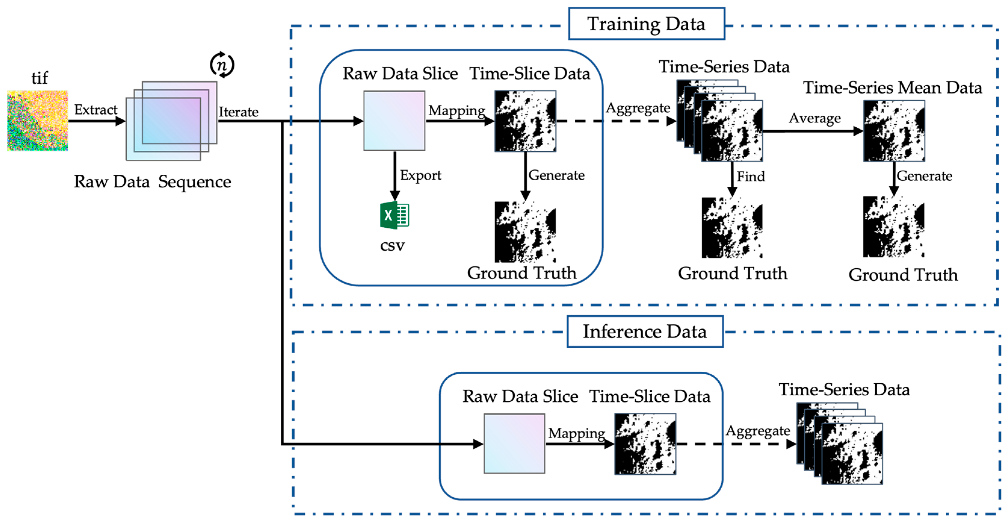
Figure 3 illustrates the workflow for generating time-slice and time-series data including both the process of training data and inference data. Initially, a TIF (Tag Image File Format) file with stacked raw data is loaded and converted into a sequence of data slices, each with a calculated Sun Visibility Factor (SVF). In the processing sub-workflow of the training data, an iteration process exports each slice to a CSV (Comma-Separated Values) file, mapping it to a 2.5D time-slice grid image and generating its ground truth mask. Following this, time-series data for model training, validation, or testing is created by aggregating a fixed number of time-slice data and determining the ground truth mask via the keyframe method. In contrast, in the experiment, time-series mean data can be generated by averaging the fixed number of time-slice data and producing its ground truth mask. Further principles and formulas will be discussed in subsequent sections. However, in the processing sub-workflow of the inference data, there is no mandatory requirement to generate CSV files and the ground truth masks. If we need to further examine and evaluate the model’s performance, we can manually generate the ground truth masks for a portion of the new inference data and incorporate them into the training data.
In this study, the Sun Visibility Factor (SVF) quantifies solar disk visibility as the ratio of the unobstructed area to the total area. This ratio ranges from 0, indicating complete obstruction, to 1, which signifies full visibility. The Sun-synchronous illumination training dataset comprises a total of 9928 image–mask pairs collected from 1 November to 30 November 2026, in the south polar area, divided into two subsets: The primary subset includes 8464 illumination data slices at 5 min intervals, while the supplementary subset contains 1464 slices at one-hour intervals. Additionally, there is an independent inference dataset comprising thousands of illumination images at 5 min intervals collected from 1 February to 28 February 2027, in the same area. Each data slice has a resolution of 20 m per pixel, dimensions of 65 × 65 pixels per image, and the same ROI in Figure 2.

2.2. Data Preprocessing Pipeline

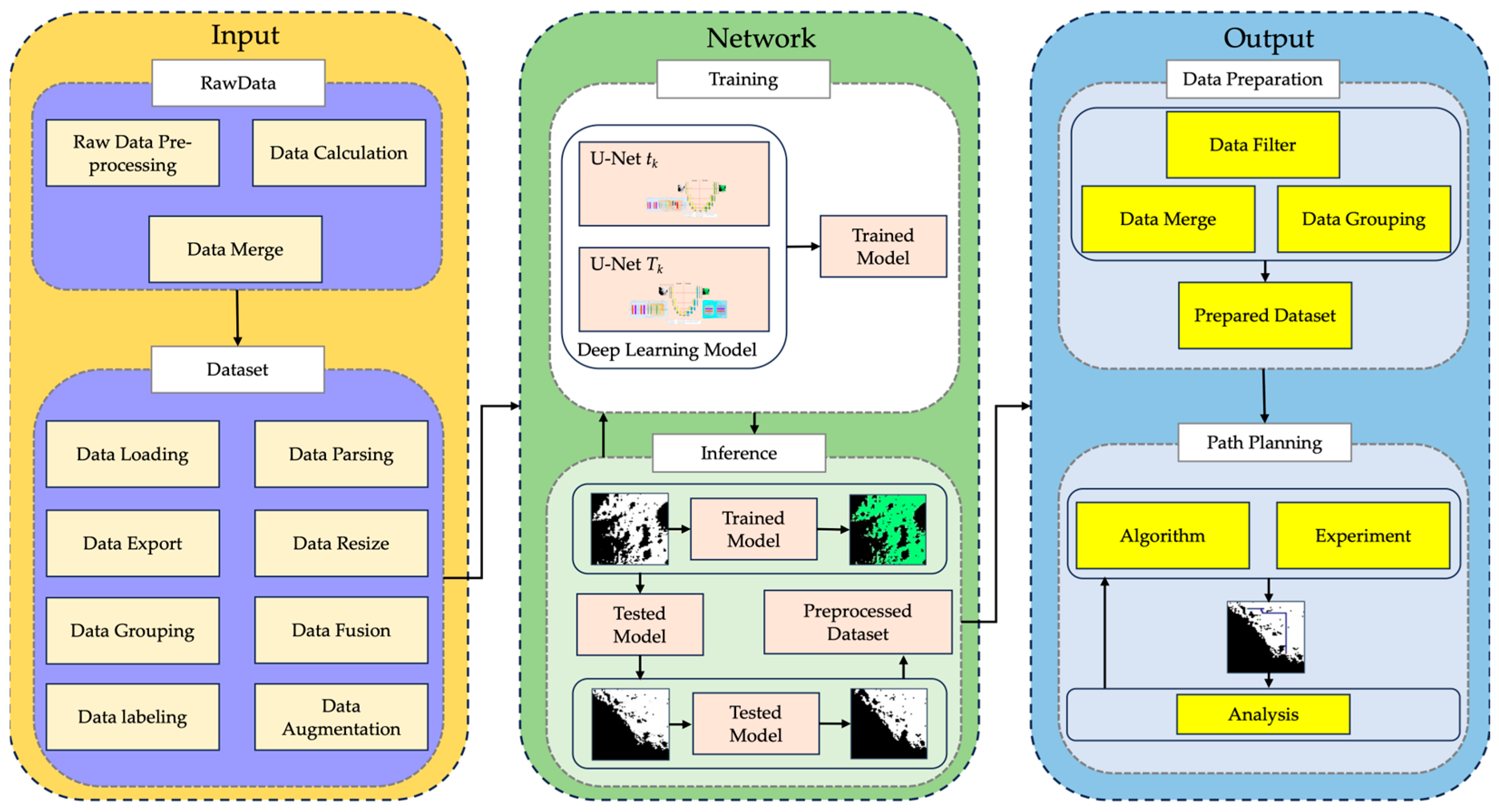
We developed a 2.5D data preprocessing pipeline that organizes various core data nodes, as illustrated in Figure 4. This pipeline encompasses acquiring and calculating raw data, centralized dataset processing, machine learning-based end-to-end processing, and the application of data in path-planning algorithms. Notably, the implementation of a Sun-synchronous spatiotemporal U-Net network, utilizing polar illumination data’s dynamic characteristics, has significantly improved the pipeline’s automation and intelligence, reducing reliance on expert experience and the costs associated with hard-coding maintenance.
The pipeline mainly consists of three parts: input, network, and output. The input part mainly focuses on raw data and datasets. It uses high-resolution DEM data, combines information such as ephemeris tables, and applies computer technologies for preliminary processing like fine-grained data calculation and merging. In the dataset, computer technology is utilized to automate various requirements for the processed data obtained from the calculation, such as data loading, parsing, exporting, grouping, and labeling. The network part mainly focuses on model training and inference. In the training block, a Sun-synchronous spatiotemporal U-Net known as 3STU-Net consists of two sub-U-Net networks that are constructed according to the time-slice and time-series characteristics of 2.5D illumination data to train semantic segmentation models of friendly illumination data under different research conditions. In the inference block, the focus is on using the tested models to conduct centralized segmentation processing of illumination data and generate new datasets (related content will be elaborated in detail in the next section). The output part mainly focuses on data preparation and path planning. Data preparation work, such as data merging and grouping, is completed according to the data requirements of path planning. In the path-planning block, research and experiments on algorithms are mainly carried out, the experimental results are analyzed, and iterations are performed. This study focuses on the research and processing of an improved Sun-synchronous spatiotemporal A* algorithm referred to as 3ST-A*. This algorithm is based on either preprocessed illumination data or alternative methods, enhancing path planning effectiveness.
Both data segmentation and the path-planning algorithm are core components of this pipeline, representing the ability to extract illuminated areas during data preprocessing and the research achievements of the path-planning algorithm. They will be discussed in the next sections.

2.3. Sun-Synchronous Spatiotemporal U-Net (3STU-Net)

The dataset is generated by integrating segmented data from various temporal sampling points into a cohesive spatiotemporal framework, as previously discussed. This integration ensures a comprehensive understanding of the data’s dynamics over time. When addressing data segmentation requirements, two prevalent scenarios emerge: The first involves segmenting data at a specific temporal instance under optimal illumination conditions, known as time-slice 2.5D data. These data are organized sequentially along the dynamic illumination time axis. The second scenario involves a temporal duration characterized by continuous time slices, referred to as time-series 2.5D data. Our research utilizes a one-hour time-series dataset comprising 12 5 min time slices, derived from the primary dataset. We perform feature fusion by aggregating data from these consecutive time slices along the temporal axis, generating a new set of time-period slice data. That is, for the input data sample F s v f and its data element in the style of SVF f i , we have
F s v f =   f i , t k                                                                                                   i , k N   f i , T k             i , k , n N ,   T k = t k , n , n 1 , 12 ,                                                                              
where f i , t k denotes the SVF value for pixel i at time slice t k , k represents the sequence number of a time-slice or time-series sample, and N represents the set of natural numbers and N = { 0 , 1 , 2 , 3 } ; f i , T k denotes the SVF value for pixel i at time series T k and n represents the number of time slice in one time-series sample T k .
Considering the mapping relationship between the RGB information of the image and SVF, we have
F g r a y = g i , t k = 255 f i , t k                     i , k N   g i , T k = 255 f i , T k                       i , k , n N ,   T k = t k , n , n 1 , 12        
where g i , t k denotes the RGB channel value for pixel i at time slice t k and g i , T k denotes the RGB channel value for pixel i at time series T k . Next, we use F t k to represent the corresponding dataset under the condition of the time slice and F T k to represent the corresponding dataset under the condition of the time series.
The 3STU-Net architecture consists of two specialized sub-networks: one for processing 2.5D time-slice data and the other for handling 2.5D time-series data. Our objective is to create sub-models that autonomously process input data from distinct scenarios and accurately segment illumination-friendly regions. This segmentation can be performed either temporally, on a slice-by-slice basis, or periodically over extended durations, requiring minimal expert knowledge or predefined maintenance protocols. Before detailing the architecture, it is crucial to quantitatively define the term “illumination-friendly”. For effective solar power utilization in lunar polar exploration, a pixel in the ROI is considered “illumination-friendly” if it receives over 75% of solar disk energy, meaning the SVF value must be at least 0.75. We assert that by adhering to this strict criterion, we can ensure that illumination conditions fulfill engineering requirements for optimal path planning.

2.3.1. 3STU-Net-1 for Time-Slice 2.5D Data

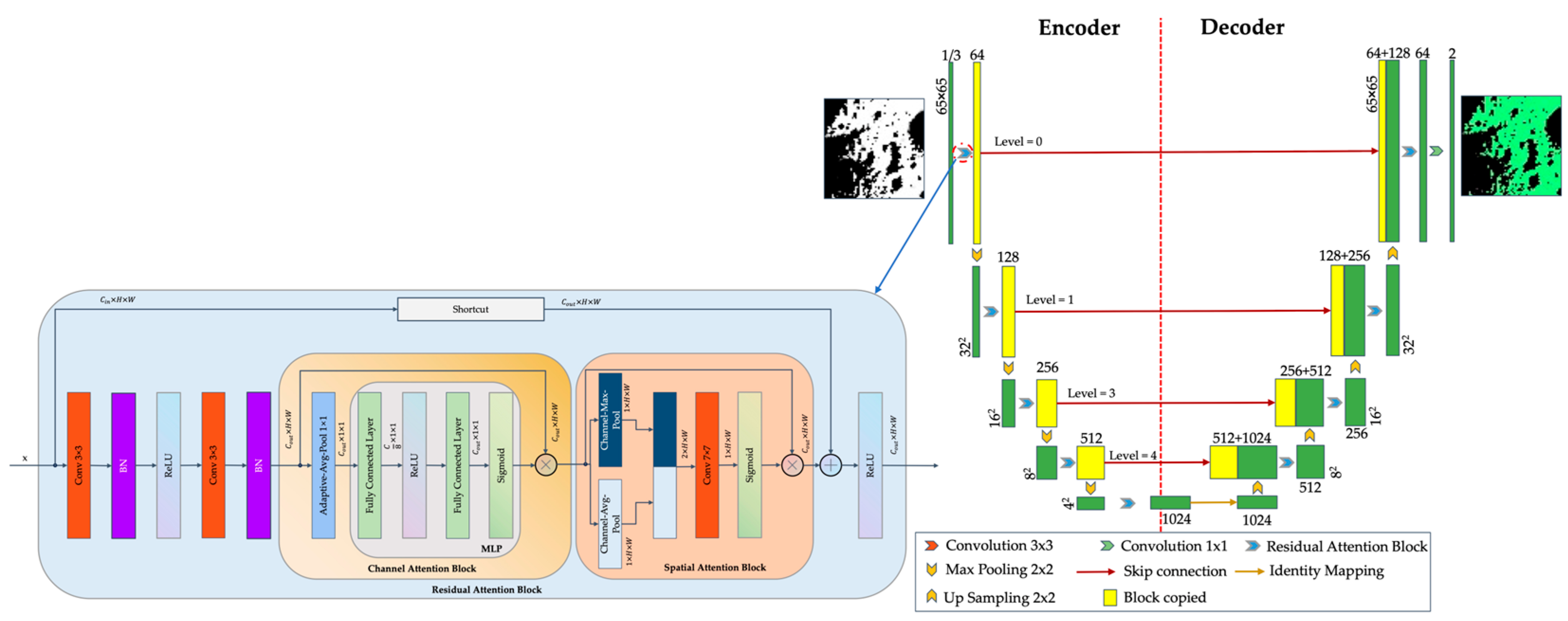
For dataset F t k , the network must master fine-grained feature extraction from 2.5D illumination time-slice data while maintaining performance balance. We have refined the original U-Net architecture by incorporating residual operations and an attention mechanism, creating an advanced framework specifically designed for time-slice 2.5D data (see Figure 5).
1. Architecture
The architecture integrates attention mechanisms with residual connections to enhance illumination feature extraction and segmentation performance. It is adaptable, allowing adjustments based on the number of input channels and classes to suit various tasks, and comprises multiple core modules.
  • “Channel Attention” Block: This block serves to enhance the responses of significant feature channels. It employs adaptive average pooling to reduce the spatial dimensions of the input feature map to 1 × 1. Subsequently, it determines the channel weights through a Multi-Layer Perceptron block, which comprises two fully connected layers interspersed with a rectified linear unit and incorporates a Sigmoid function. During the forward propagation process, the input feature map is initially pooled and flattened. The channel weights are then derived from the fully connected layers. Ultimately, the weights are expanded to correspond with the original shape of the input and are multiplied element-wise with the input, thereby augmenting the feature representation of critical channels.
  • “Spatial Attention” Block: This module executes average and maximum pooling operations on the input feature map within the channel dimension to optimize the extraction of static features. After the concatenation of the resultant outputs, it derives the weights via a 7 × 7 convolutional layer followed by the application of the Sigmoid function.
  • “Residual Attention” Block: This block comprises two groups of 3 × 3 convolutional layers accompanied by a batch normalization layer interspersed with a rectified linear unit. Subsequently, it integrates the aforementioned two attention mechanisms and incorporates residual connections to enhance the model’s efficiency.
  • The architecture’s encoder comprises “Down” modules that integrate a max-pooling layer alongside a “Residual Attention” block for down-sampling. This configuration methodically diminishes the dimensionality of the feature map while concurrently augmenting the channel count. In contrast, the decoder is structured with “Up” modules, which incorporate a transposed convolutional layer and a “Residual Attention” block to facilitate up-sampling. This process systematically enlarges the feature map’s dimensions whilst reducing the number of channels. During the up-sampling phase, the architecture adeptly addresses the discrepancies in size by concatenating the feature maps corresponding to the layers in the encoder. Ultimately, the “Out-Conv” module employs a 1 × 1 convolution to produce the segmentation results.
2. Formulation
The relevant formulas involved in this sub-3STU-Net for time-slice data X t k are summarized as follows:
  • The formula of the “Channel Attention” block is
A c X t k = δ W 2 R e L U W 1 G A P X t k                      
where X t k is the input of time-slice data, G A P represents the global average pooling operation, and W 1 and W 2 are the weight parameters of the two fully connected layers, respectively. δ represents the Sigmoid function to map the output of the attention weight values to the range of [0, 1] and the results are represented as A c X t k .
  • The formula of the “Spatial Attention” block is
A s X t k = σ C o n v C o n c a t G M P X t k , G A P X t k    
where G M P represents the global max pooling operation, C o n c a t represents the concatenating operation, C o n v represents the 7 × 7 convolutional operation, and the attention weight results are represented as A s X t k . Other characters maintain the same operation meaning.
  • The formula of the “Residual Attention” block is
R e s A t t e n X t k = R e L U P X t k + G X t k
where P X t k represents the output feature map from the main path, G X t k represents the output of the residual path, and R e L U represents the rectified linear unit operation. The formula of P X t k is
P X t k = M X t k A c X t k A s X t k          
M X t k represents the output feature map from the previous main path and its formula is
M X t k = B N C o n v R e L U B N C o n v X t k
where B N represents the batch operation, C o n v represents the 3 × 3 convolutional operation, represents the element-wise multiplication operation, A c X t k represents the “Channel Attention” block operation, and A s X t k represents the “Spatial Attention” block operation.
  • The feature update formula for each level in the encoder is
X t k l + 1 = R e s A t t e n d o w n X t k l                   l = 0 , 1 , 2 , 3
where d o w n represents the down-sampling max-pooling operation, X t k l is the feature map of the previous low layer, and X t k l + 1 is the feature map of the corresponding high layer both in the encoder.
The feature update formula for each level in the decoder is
X t k l = R e s A t t e n u p X t k l + 1 , X t k l                           l = 0 , 1 , 2 , 3
where u p represents the up-sampling transposed-convolutional operation. X t k l + 1 is the feature map of the previous high layer in the decoder and X t k l is the feature map of the corresponding low layer in the encoder.
3. Ground Truth Mask
The ground truth mask for each data slice is made based on the “illumination-friendly” threshold: 1 for SVF > 0.75 and 0 for otherwise.

2.3.2. 3STU-Net-2 for Time-Series 2.5D Data

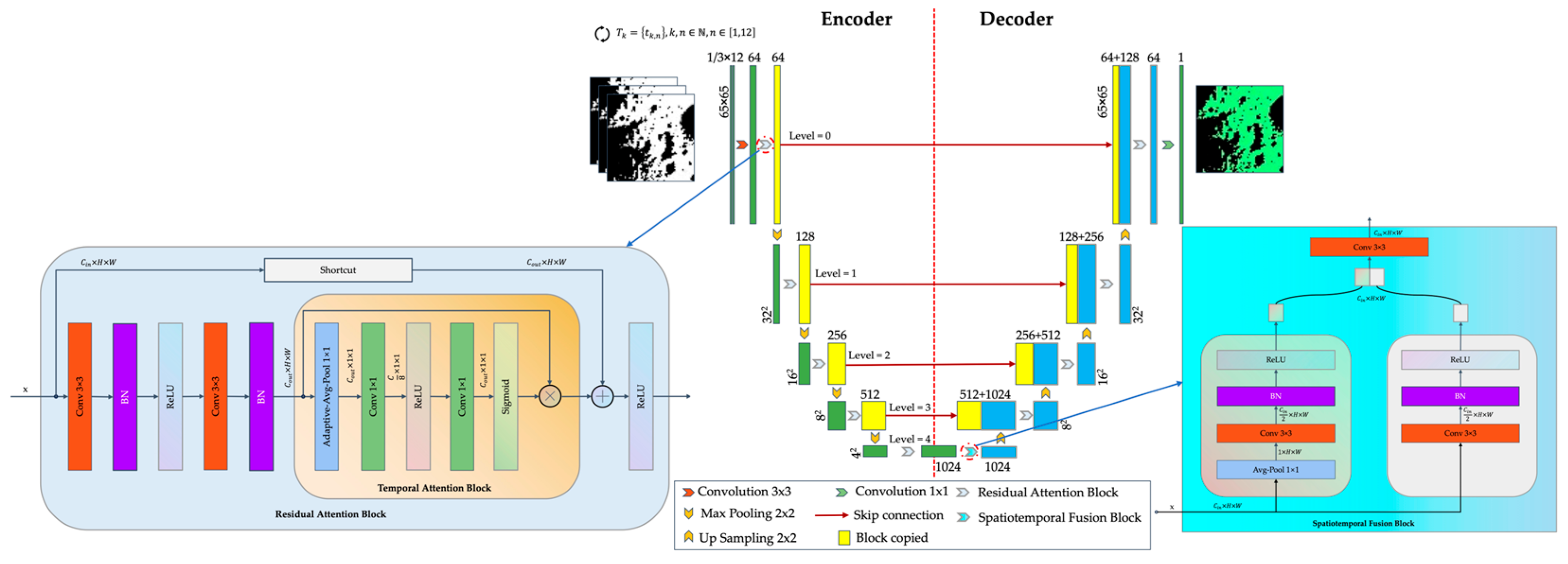
In the context of sample F T k , the network must learn feature fusion and extraction capabilities from 12 time-slice samples while ensuring optimal performance. Building on 3STU-Net-2’s design, we enhance time-series data processing by capturing dynamic variations through data aggregation and averaging. Additionally, we extract spatial static features from each slice and present an improved U-Net architecture for time-series 2.5D data, as shown in Figure 6.
1. Architecture
The architecture integrates the attention mechanism with residual connections, enhancing illumination feature extraction and segmentation performance. It can be adjusted based on input channels and class numbers for various tasks. Targeted improvements are made on the time-slice U-Net architecture modules, leading to the proposal of relevant core modules.
  • “Input Layer” block: This block enhances input features by using a 3 × 3 convolutional layer to convert input channels into 64 channels, extracting basic features such as edges and textures. It is then processed by a custom residual convolution block, known as the “Residual Attention” block, which will be introduced later. The residual connection alleviates the vanishing gradient problem and improves feature extraction.
  • “Temporal Attention” Block: This block enhances feature extraction of time slices by replacing both the “Channel Attention” and “Spatial Attention” blocks. It utilizes the channel attention mechanism, beginning with adaptive average pooling to condense the input feature map to 1 × 1, obtaining global average features for each channel. Next, two 1 × 1 convolutional operations are performed, separated by a rectified linear unit. The first convolution reduces the channel count to one-eighth of the original, thereby lowering computational complexity. The second convolution restores the channel count to its original level. The Sigmoid function then maps the output to the range of [0, 1], producing attention weights for each channel. These weights are finally multiplied element-wise with the input feature map to enhance the important channel features.
  • “Residual Attention” Block: This block enhances the temporal feature extraction ability of temporal slice data by employing a temporal attention mechanism alongside a residual connection. The primary modification involves replacing the original “Channel Attention” and “Spatial Attention” blocks with the “Temporal Attention” block, while other design elements remain unchanged.
  • “Spatiotemporal Fusion” Block: This module fuses temporal and spatial features, connecting the encoder and decoder. In the temporal branch, the input feature map is averaged along the channel dimension to create a temporal feature map, which is processed through a 3 × 3 convolutional layer with a channel constraint of 1. This is followed by batch normalization and a rectified linear unit, resulting in a feature map with half the input channels. In contrast, the spatial branch retains its structures without the average pooling in the channel dimension, emphasizing static spatial features. Finally, the temporal and spatial feature maps are concatenated along the channel dimension and processed through another 3 × 3 convolutional layer for effective feature fusion.
  • The designs of the other parts of the encoder and decoder of this architecture are the same as those for time-slice data. The improved “Residual Attention” block is placed in each layer for refined feature extraction. Ultimately, the “Out-Conv” module uses a 1 × 1 convolution to output the segmentation result.
  • The encoder and decoder designs in this architecture mirror those used for time-slice data. Each layer incorporates an enhanced “Residual Attention” block for improved feature extraction. Ultimately, the “Out-Conv” module employs a 1 × 1 convolution to produce the segmentation results.
2. Formulation
The relevant formulas involved in this 3STU-Net-2 for time-series data X T k I n p u t are summarized as follows:
  • The formula of the “Input Layer” block is
    X T k l = 0 = R e s A t t e n C o n v X T k I n p u t              
    X T k l = 0 is the output feature map of the input layer, C o n v represents the 3 × 3 convolutional operation, and R e s A t t e n represents the “Residual Attention” block operation, which we will discuss later. X T k I n p u t is the input of time-series data.
  • The formula of the “Temporal Attention” block is
    A T ( X T k ) = δ ( C o n v ( R e L U C o n v ( G A P X T k ) ) )            
    where G A P represents the global average pooling operation. C o n v represents the 1 × 1 convolutional operation. R e L U represents the rectified linear unit operation. δ represents the Sigmoid function to output the attention weight values to the range of [0, 1] and the results are represented as A T ( X T k ) .
  • The formula of the “Residual Attention” block is
    R e s A t t e n X T k = R e L U P X T k + G X T k
    R e L U represents the rectified linear unit operation. P X T k represents the output feature map from the main path and G X T k represents output of the residual path. The formula of P X T k is
    P X T k = M X T k A T X T k    
    M X T k represents the output feature map from the previous main path, and its formula is
    M X T k = B N C o n v R e L U B N C o n v X T k
    where B N represents the batch operation. C o n v represents the 3 × 3 convolutional operation. represents the element-wise multiplication operation. A T X T k represents the “Temporal Attention” block operation. The formula of G X T k is
    G X T k = C o n v X T k , C i n C o u t X T k ,   o t h e r w i s e
The goal of this formula is to ensure that the data output by the shortcut operation meets the corresponding value requirements of the residual output.
  • The formula for the “Spatiotemporal Fusion” block is
F X T k = C o n v C o n c a t R e L U B N C o n v G A P X T k , R e L U B N C o n v X T k
where C o n c a t represents the concatenating operation and C o n v represents the 3 × 3 convolutional operation. Other characters maintain the same operation meaning as mentioned before.
  • The feature update formula for each level in the encoder is
X T k l + 1 = R e s A t t e n d o w n X T k l           l = 0 , 1 , 2 , 3
where d o w n represents the down-sampling max-pooling operation. Between the encoder and the decoder, the “Spatiotemporal Fusion” block, which is represented by Formula (16), needs to be invoked to perform fusion processing on the spatiotemporal data. This part mainly deals with the data X T k 4 that are the final output of the encoder and transmit values into the decoder network represented by Formular (18). The feature update formula for each level in the decoder is represented by Formular (19):
X T k 4 = F X T k 4
X T k l = R e s A t t e n u p X T k l + 1 , X T k l           l = 0 , 1 , 2 , 3
where u p represents the up-sampling transposed-convolutional operation. X T k l + 1 is the feature map of the previous layer in the decoder and X T k l is the feature map of the corresponding layer in the encoder.
3. Ground Truth Mask
The ground truth mask for each series is determined by the “illumination-friendly” threshold: a value of 1 for SVF > 0.75 and 0 otherwise. To effectively obtain the ground truth mask, we employ the keyframe method, selecting the middle slice of each series to balance accuracy and performance.

2.3.3. Loss Function

Compared with other types of U-Net, the 3STU-Net in this paper focuses on the fine extraction and segmentation ability of the polar illumination-friendly areas. While giving priority to optimizing the ability of global illumination extraction and segmentation, it also needs to take into account the ability to extract illumination information in local areas, boundary areas, and intersection areas. Therefore, it is necessary to consider the comprehensive optimization ability in these two aspects. Since the cross-entropy loss function mainly focuses on global optimization [66], and the Dice loss function focuses on local optimization [67], this paper adopts a hybrid loss function composed of the cross-entropy function and the Dice loss function to optimize the model.
The general formula for the hybrid loss L t o t a l is
L t o t a l = α L C E + 1 α L D i c e
where L C E is the cross-entropy loss, L D i c e is the Dice loss, and α is a hyperparameter used to balance the weights of two losses. The calculation for the cross-entropy loss is
L C E = 1 N i = 1 N k = 1 2 y i , k log p i , k                 y i , k 0 , 1
where y i , k represents the one-hot encoding of the ground truth label for pixel i , which is the true illumination condition classification ( k = 1 for the illumination-friendly area, and k = 0 for the illumination-unfriendly area). p i , k is the probability of the illumination condition classification predicted by the model and N is the total number of pixels. The calculation for the Dice loss is
L D i c e = 1 2 k = 1 2 i = 1 N y i , k p i , k + ϵ k = 1 2 i = 1 N y i , k + p i , k + ϵ
where ϵ is a small constant used for numerical stability, and its main function is to avoid division by zero errors and illegal inputs in logarithmic operations.

2.3.4. Assessment

In this paper, the evaluation metrics for the model mainly include accuracy and mean intersection over union ( m I o U ). These two metrics are used to mainly reflect the performance of the model in the semantic segmentation of spatiotemporal characteristic illumination data.
Accuracy is a widely used metric for evaluating model performance. In classification tasks, it is used to measure the proportion of correctly predicted samples by the model in the total number of samples. The formula is
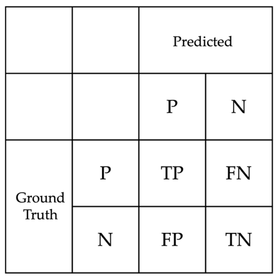
A c c u r a c y = T P + T N T P + T N + F P + F N
Here, we consider the illumination-friendly condition as the positive class (P) and the illumination-unfriendly cases as the negative class (N). The meanings of the characters in Formula (23) are shown in Figure 7.
I o U is a commonly used evaluation metric in semantic segmentation tasks, representing the degree of overlap between the predicted region and the ground-truth region. The formula is shown as (24), where y i , c represents the ground truth label for pixel i and class c , while q i , c represents the predicted label for pixel i and class c .
I o U c = I n t e r s e c t i o n y , q U n i o n y , q = i = 1 y i , c q i , c + ϵ i = 1 y i , c + i = 1 q i , c i = 1 y i , c q i , c + ϵ           c 0 , 1
m I o U is the average value of I o U , representing the average of I o U s for all classes, as shown in Formula (25).
m I o U = 1 2 C = 1 2 I o U C

2.4. Sun-Synchronous Spatiotemporal A* Path-Planning Algorithm (3ST-A*)

2.4.1. A* and Spatiotemporal A* (ST-A*)

The A* path-planning algorithm is a heuristic search algorithm used to find the optimal path in grid-based maps. It comprehensively takes into account the actual cost from the starting point to the current point and the estimated cost from the current point to the target point. It guides the search direction through a heuristic function f n and can efficiently find the shortest path or the optimal path from the starting point to the ending point by minimizing the f n for each node in the path [68,69]. The formula of f n is
f n = g n + h n
where n represent the node for estimating, g n is the actual cost from the starting node to node n and g n s = 0 for start node, and h n is the estimated cost from node n to the target node, which is usually calculated using heuristic functions such as the Manhattan distance, Euclidean distance, etc.
Spatiotemporal A* or ST-A* is an extension of the A* path-planning algorithm. Based on the traditional A* algorithm that considers spatial information, it incorporates the time dimension, calculates costs by integrating spatial location and time factors, and is used to find the optimal path in a dynamically changing environment [53]. In addition to non-time-varying spatial factors such as slopes and obstacles, environmental factors like illumination change dynamically over time. Thus, the spatiotemporal map information faced during each step of path planning is different, and the planned path cannot be dynamically adjusted. This makes the traditional A* algorithm based on static spatiotemporal information unable to handle such problems. Currently, one of the main research directions of spatiotemporal A* is to improve the algorithm by introducing the time dimension and fusing non-variable and variable spatiotemporal data based on the traditional algorithm. However, it also faces research challenges such as low-resolution datasets and complex cost functions [53,54].

2.4.2. 3ST-A*

This paper supports research on the data preprocessing pipeline by implementing an enhanced ST-A* algorithm. Utilizing slope and dynamic illumination data on 1 km × 1 km polar grid maps, we propose the 3ST-A* (Sun-Synchronous Spatiotemporal A*) path-planning algorithm, characterized by a simple cost function derived from high-spatial-resolution data.
1.
Maps
This algorithm uses non-time-varying slope and time-varying illumination 2.5D grid-based maps in the same area, where slope or illumination data are appended vertically to the 2D coordinates. Let the slope map data be S s l o p e , and the illumination data be divided into time slice F t k and time series F T k , where data are arranged in chronological order to form a data sequence. It denotes the node as n , the current point as n i , the starting point as n s , and the goal point as n g .
For the time series F T k , in the case of no fusion processing of time series by 3STU-Net, we define that a single sample data f T k is processed as the average of N time-slice data, that is
f i , T k = 1 N i = 0 N f i , t k
The rule for generating its ground truth mask follows the same rules as the time-slice data by using the mean data.
2.
Fixed Path Route
Since the illumination data varies at each time point, the explored paths need to be fixed and recorded. In this algorithm, the open set is stored in the form of ( f n e , n e ) . Beginning from the starting point, the algorithm extracts the node with the minimum cost f n e from the searched neighbor nodes and saves it into the closed set. Then, before searching for the next neighbor node, the open set is emptied, and the optimal neighbor node search is carried out. This ensures that the already planned nodes are only related to the current node, achieving the fixation of the planned route.
3.
Cost Function
For a neighbor node n e of the current node n i at each searching time, the cost function of 3ST-A* is to ensure that, through searching the minimum value of the heuristic function f n e , while selecting nodes are illuminated and suitably sloped areas, the ability to search for the next node by using the Euclidean distance is retained. The formulas are
f n e = g n e + h ( n e ) g n e = g n i + d i s n i , n e h ( n e ) = d i s n e , n g + h s l o p e ( n e ) + h i l l ( n e , f n e , t k ) / h i l l ( n e , f n e , T k )  
where h ( n e ) is the function that is mainly different from the original A* algorithm, which is composed of the estimated cost of the Euclidean distance d i s n e , n g from the neighbor node to the target node, the estimated slope cost of the neighbor node h s l o p e ( n e ) , and the estimated illumination cost h i l l ( n e , f n e , t k ) / h i l l ( n e , f n e , T k ) . The value of h s l o p e ( n e ) is defined as follows:
h s l o p e n e = 0                   s n e < s l o p e _ t h r e s h o l d +                                                                 o t h e r s
where the slope threshold in this algorithm is 20 ° . The value of h i l l ( n e , f n e , t k ) / h i l l ( n e , f n e , T k ) is defined as follows:
h i l l ( n e , f n e , t k ) / h i l l ( n e , f n e , T k ) = +                 f n e , t k / f n e , T k   i s   d a r k 0                                                                   o t h e r s
where the dark refers to the SVF f n i , t k / f n i , T k   , and for the neighbor node, n e is 0. The g n e is the actual cost function, which is composed of the actual cost of the current node g n i and the actual cost of the Euclidean distance d i s n i , n e from the current node to the neighbor node.
Finally, we give the main process of the 3ST-A* algorithm in Table 1.
4.
Assessment
This paper introduces two additional criteria for evaluating the algorithm: the number of illumination grid conditions (NoI) and the number of slope grid conditions (NoS). These criteria complement the existing metrics of steps and time required for path planning in the Sun-synchronous scenario. Detailed information is provided in Table 2.

3. Experiment Setup

The experimental setup comprises two main components: 3STU-Net and 3ST-A*. We implemented all algorithms and pipeline modules using Python 3.10 and the PyTorch 2.6.0 library. Experiments were conducted on an Intel® Arc™ Graphics GPU (XPU) with 18 GB of memory and 22 Intel® Core™ Ultra CPUs.

3.1. 3STU-Net

The experimental section on the 3STU-Net focuses on model training and performance verification. We compare the 3STU-Net-1 model with the original U-Net and Attention U-Net. In contrast, the 3STU-Net-2 network processes 12 time-slice data simultaneously for feature fusion, complicating direct comparisons. To enable comparison, we calculate the average of every 12 time-slice data using Equation (27) as the input for both U-Net models. The dataset comprises three parts: 70% for training, 20% for validation, and 10% for testing, with all input data resized to 65 × 65. Detailed hyperparameters for the 3STU-Net model training are available in Table 3.
To optimize computing resource usage and facilitate comparison, we configured different hyperparameters for the original U-Net and Attention U-Net. Both models use a batch size of 4 and the cross-entropy loss function, employing the Adam optimizer with a learning rate of 0.0002.

3.2. 3ST-A*

This study focuses on various path-planning scenarios of 3ST-A*, using data derived from DEM and comparing results with and without 3STU-Net preprocessing. Details of the relevant experimental settings can be found in Table 4.
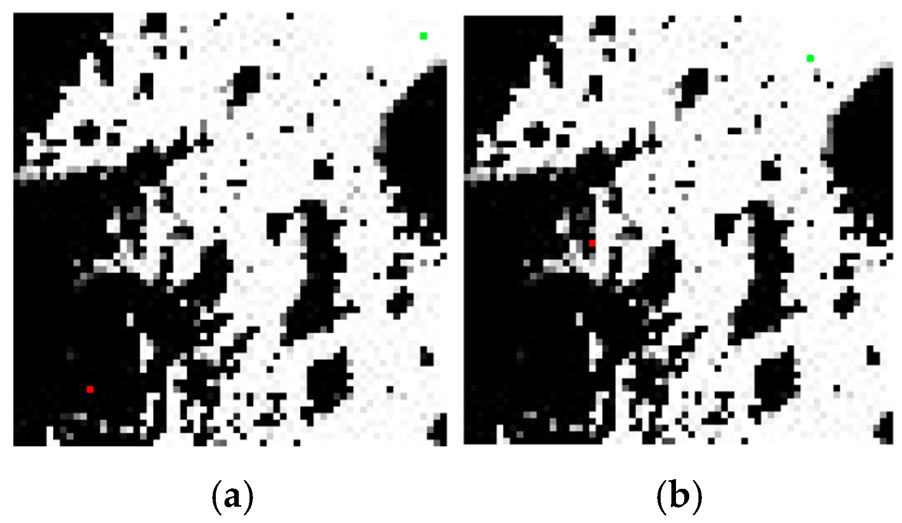
In Table 4, we examine two distinct groups of start and goal nodes, each containing 10 scenarios for comparison. The first group, illustrated in Figure 8a, spans a longer path from node a (the red dot) to node b (the green dot) and includes scenarios No. 1–6. The second group, shown in Figure 8b, focuses on a shorter path from node c to node d, incorporating scenarios No. 7–10. The data utilized in the preprocessing pipeline encompasses time-slice and time-series illumination data, including both 3STU-Net preprocessed and non-preprocessed data. Non-preprocessed time-series data are derived from the average of 12 time slices, while the preprocessed data originate from 3STU-Net-2. Due to slope condition limitations, an independent slope grid map of the same area was also incorporated into this experiment.
In this study’s context of global path planning, the rover’s motion model has been simplified to include four navigation directions, as discussed in detail in reference [55]. This simplification aids in understanding the planning process and enhances the overall effectiveness of the navigation strategy.

4. Results and Discussion

4.1. 3STU-Net Learning Results

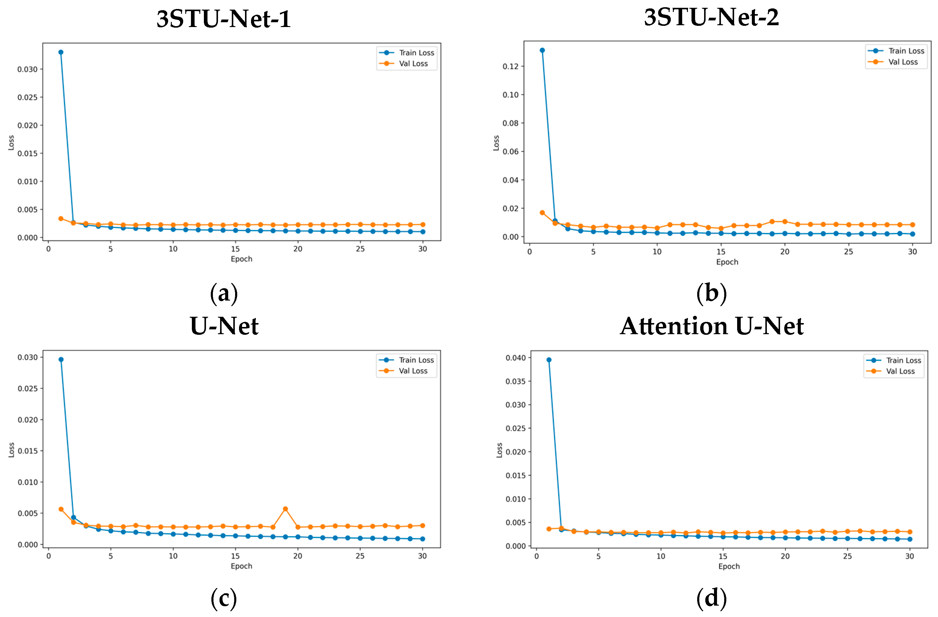
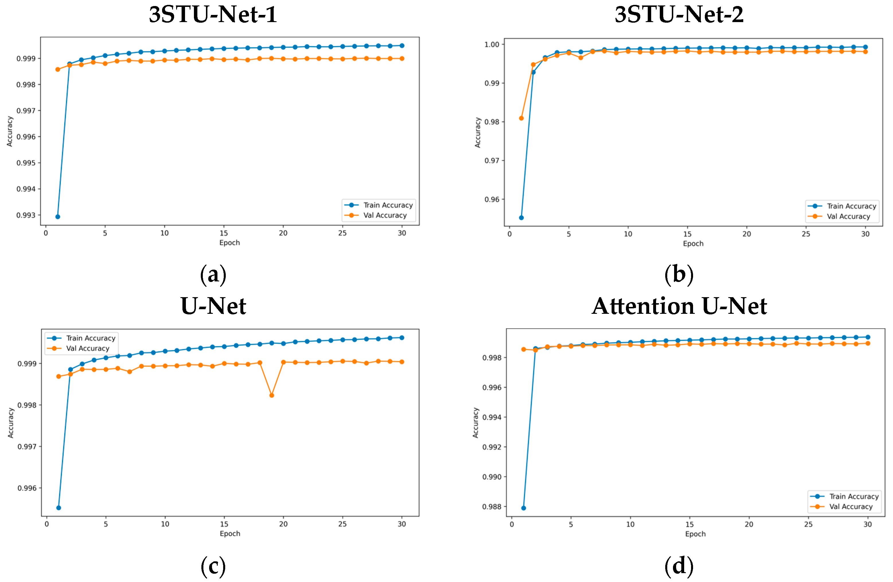
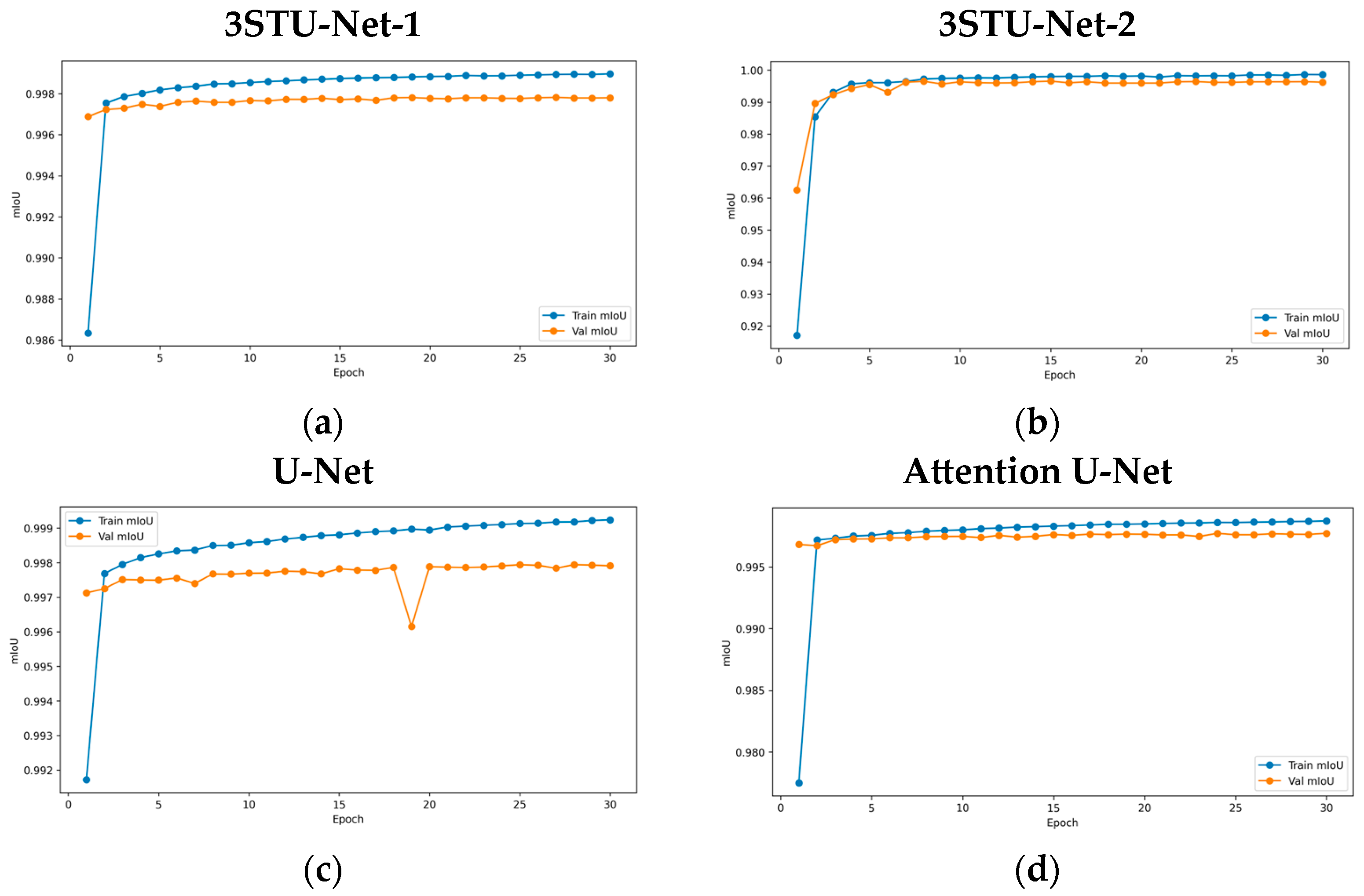
Figure 9, Figure 10 and Figure 11 display the learning curves for 3STU-Net-1, 3STU-Net-2, U-Net, and Attention U-Net, illustrating training and validation losses. The blue line indicates training loss, while the orange line shows validation loss. The curves converge after several epochs, indicating the model’s readiness for comparative analysis despite limited lunar south pole lighting data.
The test results for 3STU-Net-1, 3STU-Net-2, U-Net, and Attention U-Net were evaluated on independent testing datasets, focusing primarily on accuracy. The extracted results are summarized in Table 5.
The results in Table 5 demonstrate that the 3STU-Net significantly enhances accuracy and mIoU for both sub-networks. The 3STU-Net-1 achieved 95.01% accuracy and 87.18% mIoU, surpassing the original U-Net by 0.12% and 0.31%, respectively, and improving by 0.21% and 0.51% over Attention U-Net. For 3STU-Net-2, which processes 12 temporal time-slice data simultaneously, accuracy reached 96.44% and mIoU 91.85%. In contrast, U-Net yielded 94.99% accuracy and 89.94% mIoU, while Attention U-Net recorded 94.90% accuracy and 89.84% mIoU using averaged data. Despite different data processing methods and architectures, the model’s performance with time-series data outperformed that of time-slice data, highlighting that feature fusion from multiple slices is more effective for model segmentation.
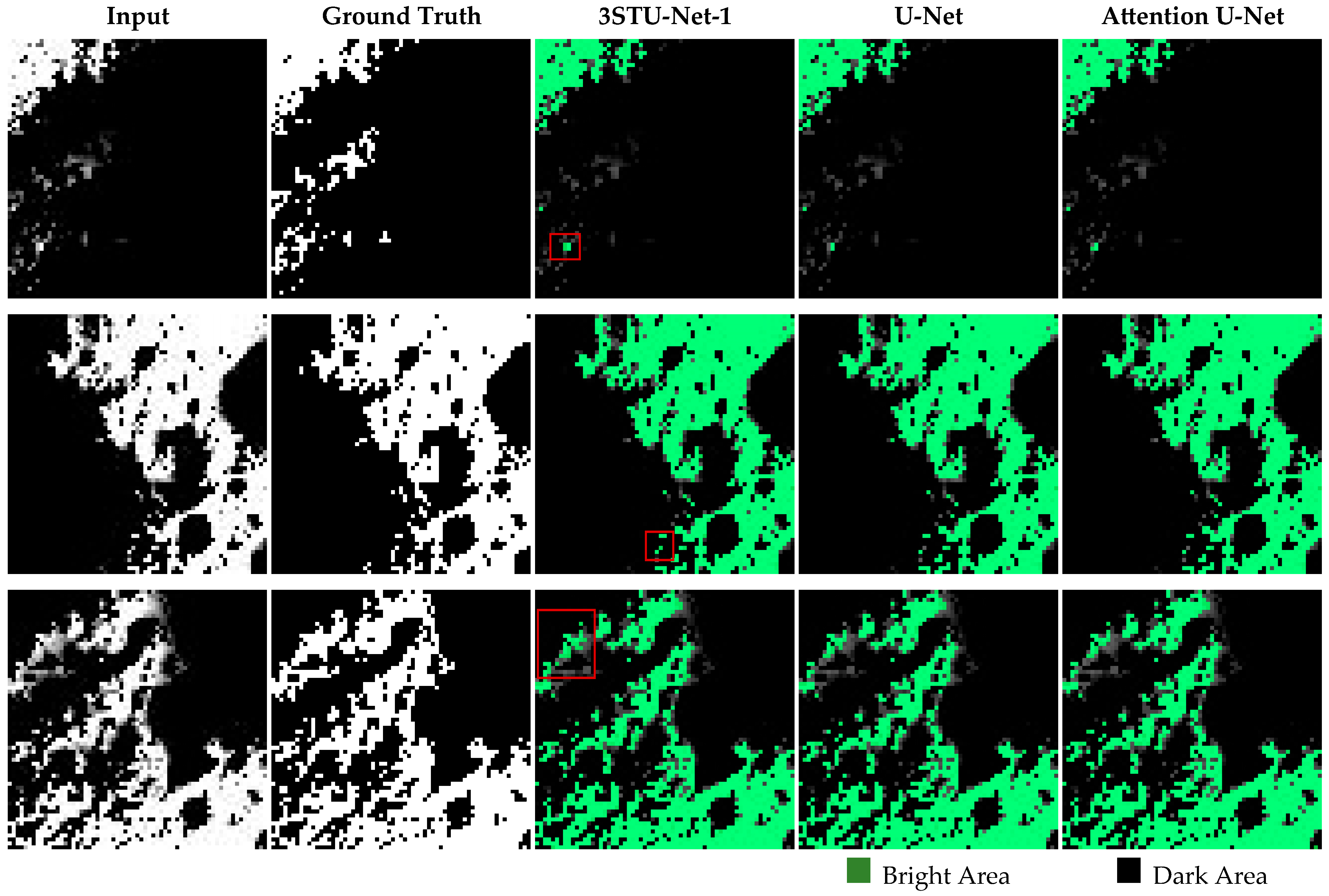
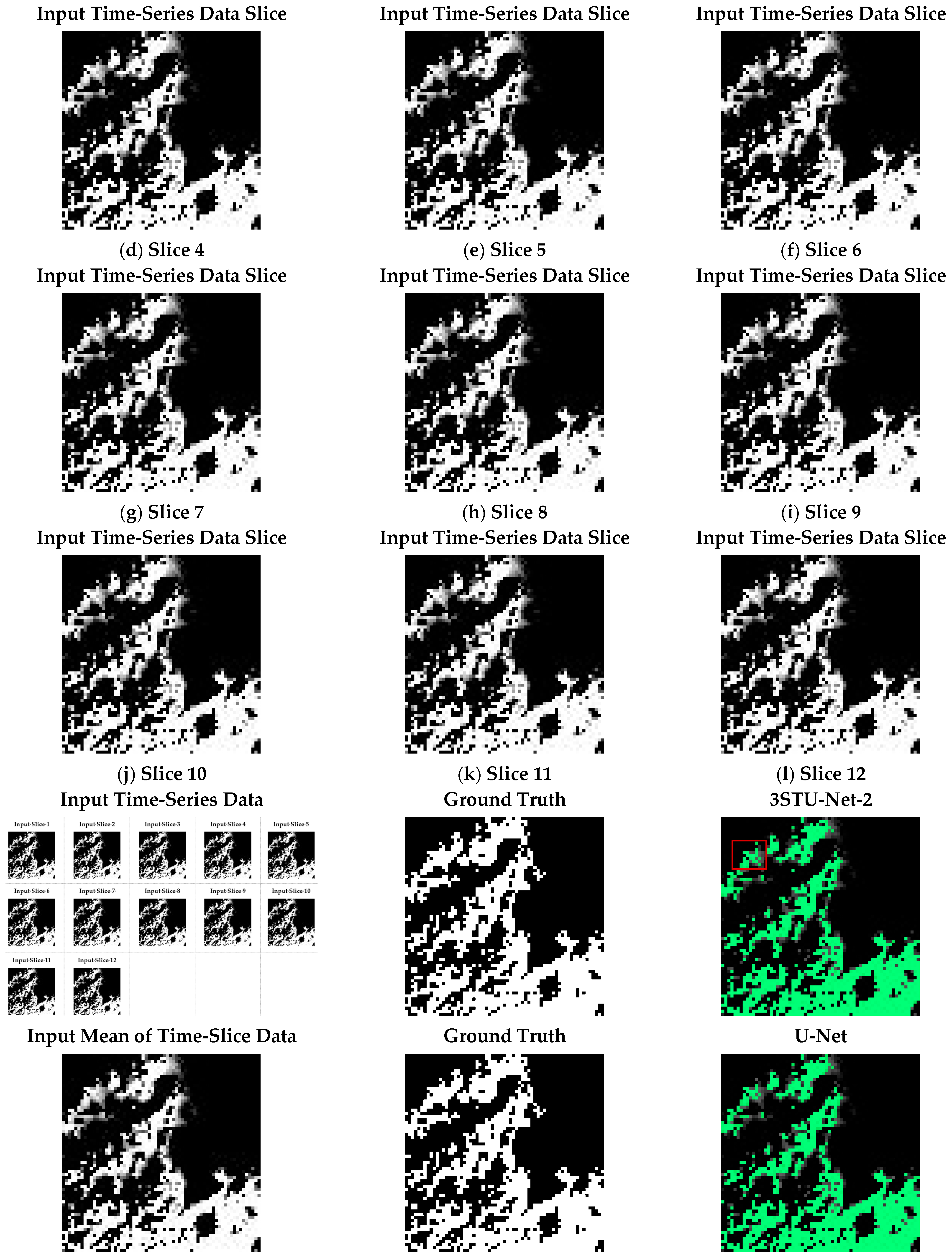
Figure 12 and Figure 13 show the comparison of results proceed by two groups: one contains the data proceed by 3STU-Net-1, U-Net, and Attention U-Net with the same input data and ground truth mask, the other contains 3STU-Net-2, U-Net, and Attention U-Net with time-series data as the input, and keyframe as the ground truth mask for 3STU-Net-2 and the mean value of the same time-series for U-Net and Attention U-Net. The subfigures with a green color shown in Figure 12 and Figure 13 were an overlay of the proceeding data marked as green and the original input data as the base background to showcase the comparison of difference between them. The comparison shows different models’ performance in marking illumination-friendly areas: In Figure 12, the green area indicates the illumination-friendly zone identified by the 3STU-Net-1 model, while the raw input data shows various illumination conditions; Figure 13 demonstrates that the 3STU-Net-2 network can directly extract illumination-friendly areas using time-series data, whereas U-Net and Attention U-Net rely on pre-calculated mean values. While 3STU-Net demonstrates superior edge detail, 3STU-Net-2 introduces a novel approach for multi-slice data fusion. However, the model struggles with extracting complex lighting areas, indicating a need for further research to improve segmentation capabilities.

4.2. 3ST-A* Path Planning Results and Comparation

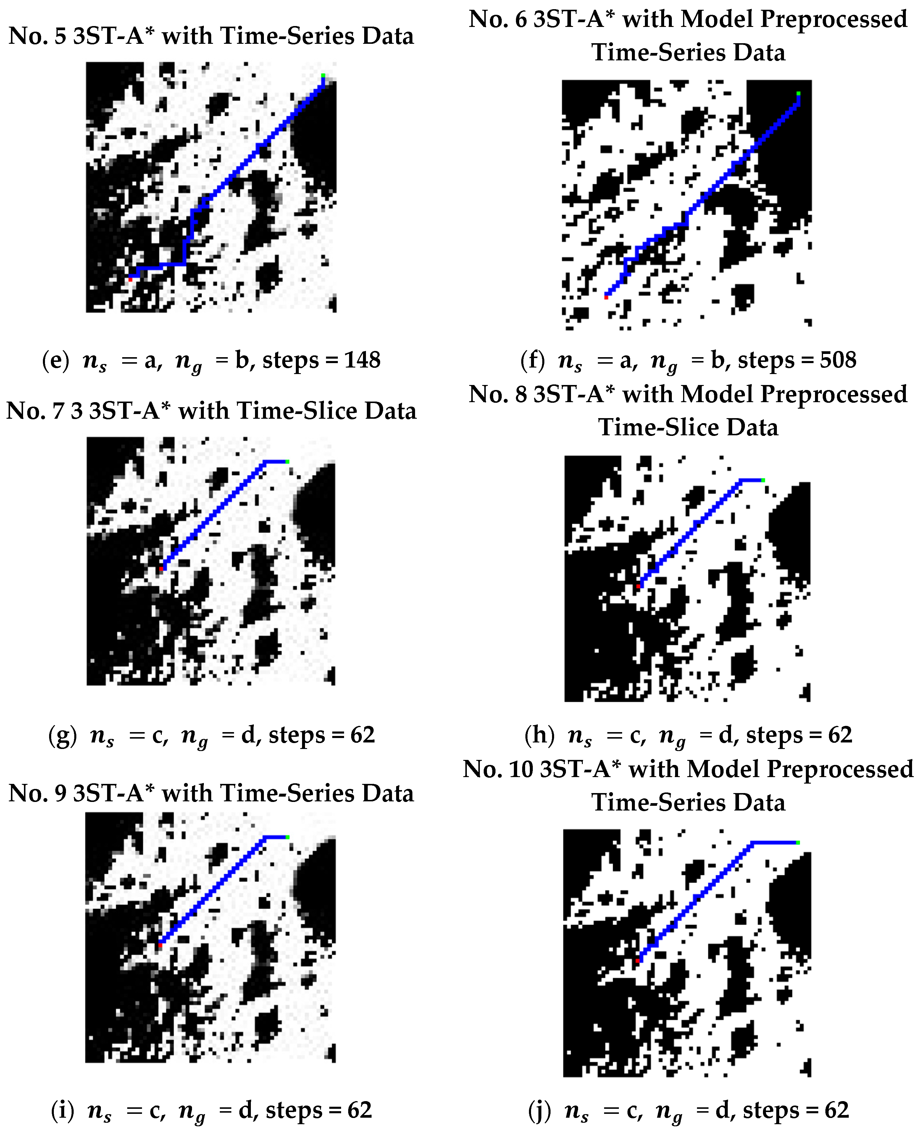
The results of the path-planning algorithm experiments, as detailed in Table 4, were carried out. The route curves are shown in Figure 14, the snapshots of key time points for path planning for scenario No. 4 are shown in Figure 15 and the related data are displayed in Table 6.
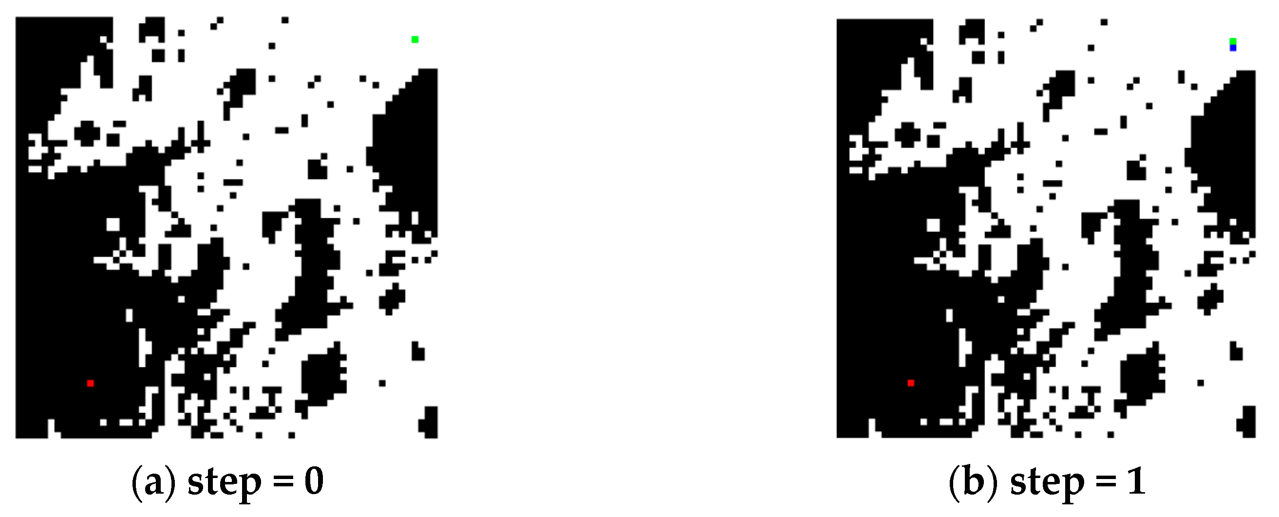
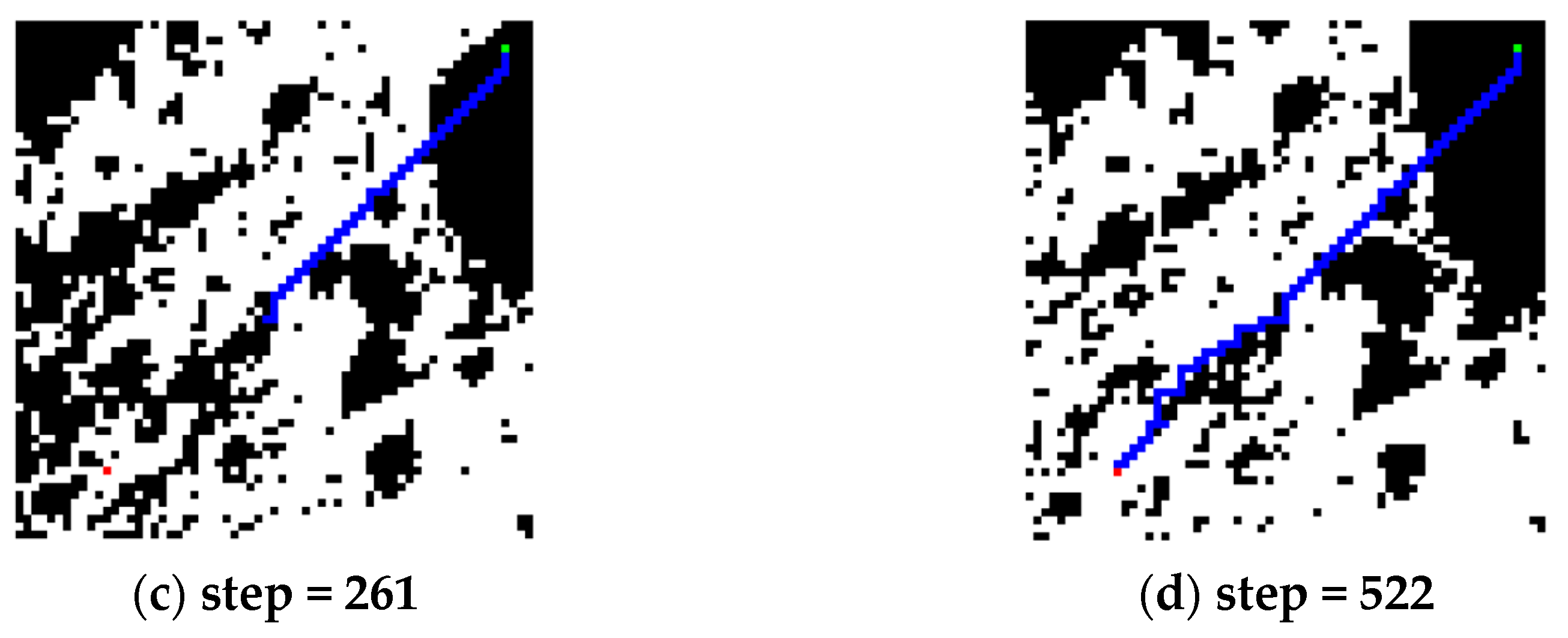
The visualizations of path-planning algorithms in Figure 14 depict the route status at the last time point. The green tile indicates the state node, the red tile indicates the goal node, and the blue line indicates the planned route trace. The time-slice data, labeled with serialized numbers, derives from either original datasets or those preprocessed using the 3STU-Net-1 model. Meanwhile, time-series data comes from original datasets calculated through Equation (27) or preprocessed with the 3STU-Net-2 model. All algorithms successfully plan a route between the start and goal nodes, with differences in planned steps and areas traversed, such as dark, weak-light, and bright zones. In scenarios using original image data (Nos. 1, 2, 3, 5, 7, 9), various lighting conditions are represented. Conversely, in cases with segmented data (Nos. 4, 6, 8, 10), only areas with an SVF above 0.75 are marked as illuminated. As shown in Table 6, the original A* algorithm (Nos. 1, 2) offers the shortest path but passes through dark and weak-light areas, failing to meet Sun-synchronous path planning requirements. The 3ST-A* algorithm effectively avoids dark areas. In unsegmented data scenarios, traces may pass through dark and weak-light areas, necessitating replanning using the 3ST-A* rechoosing approach (Nos. 3 and 5).
In Figure 15, there are four snapshots of the path planning of No. 4 in Table 4 by using the 3ST-A* with the 3STU-Net-1 model preprocessed time-slice data. From the figures, we can see that all the planned routes at each time point can ensure the rover moves in a friendly illumination condition, which is dynamically changing at every time point.
Comparing path-planning algorithms reveals that the 3STU-Net-2 fused time-series data processing effectively avoids stagnation and bypasses weak lighting areas (Nos. 5, 6, 9, 10). The mean processing of original time-slice data suffers from significant blighting data accuracy loss. In long-distance path planning (Nos. 4 and 6), the number of steps increases due to the segmentation process, which imposes additional restrictions and reduces available planning data. However, this method ensures that the selected lighting areas meet the requirements for Sun-synchronous path planning.

4.3. Discussion

An automated data preprocessing pipeline for 2.5D data significantly enhances Sun-synchronous path planning research in polar regions. The 3STU-Net network improves fine-grained segmentation for sequential time-slice data. In contrast, the original U-Net and Attention U-Net networks fail to adequately address temporal details, resulting in poor scenario adaptation and edge segmentation under complex illumination. Consequently, these models often depend on mean input time-series data, distorting information and increasing manual processing workload.
In this study, we demonstrate that the 3ST-A* algorithm facilitates dynamic path planning, allowing the rover to navigate illuminated areas effectively. By utilizing the 3STU-Net for data segmentation, the planned path remains within optimal lighting zones. Furthermore, the proposed segmentation algorithm improves path-planning accuracy through the integration of fused time-series data. The Sun-synchronous path-planning algorithm introduces additional selection constraints, extending beyond the original Euclidean distance requirement, which results in a slight increase in path steps. In the context of the flat study area, the slopes of paths from all algorithms, including the original A*, satisfy the requirements. Due to the rover motion mode in this study, the planned routes shown in Figure 14 and Figure 15 have broken lines. However, considering the actual speed of the rover, the global path planning described in this paper is first carried out rapidly based on the illumination conditions for Sun-synchronous path planning, which guides the rover in selecting the navigation direction in dynamic scenarios, providing a fast, cost-effective solution for adapting to complex changes by using 3STU-Net models and 3ST-A*. After the rover completes the local path planning in reality and travels according to the global path, new global path planning can be carried out promptly and an evaluation basis can be provided. Therefore, the single broken line has certain practical significance within the scale of 20 m/pixel resolution when it comes to providing the choice of driving direction and the main path. Certainly, future research should explore the possibility of extending path planning to cover eight or more moving directions to better meet the requirements of practical tasks.
Our methods, models, and algorithms significantly contribute to Sun-synchronous path planning, particularly in complex lighting conditions. However, the segmentation processing model needs further training to improve generalization for intricate texture features, given the limited polar region data. The enhanced A*-based path-planning algorithm relies on the cost function for identifying feasible regions, highlighting the necessity for expert input and refinement of hard coding techniques. Furthermore, adapting to changing environmental conditions for real-time path planning is crucial. Future research will focus on leveraging data preprocessing to advance learning-based Sun-synchronous path planning.

5. Conclusions

This paper investigates dynamic spatiotemporal data preprocessing for Sun-synchronous path planning in the Lunar polar regions. It presents a workflow for data preprocessing and introduces a pipeline model that standardizes spatiotemporal data processing. Central to this model is an enhanced U-Net network, 3STU-Net, designed for segmentation and classification of Sun-synchronous time-slice and time-series data. Additionally, the processed data enhanced the 3ST-A* path algorithm, improving its complexity, accuracy, and usability in path planning.
In the pipeline, the 3STU-Net facilitates fine-grained segmentation of friendly lighting areas. Key conclusions include the following:
(1)
A residual module enhances feature extraction for time-slice data through a channel attention mechanism.
(2)
Twelve consecutive time slices are used for time-series data, employing a residual attention module that combines a temporal attention block and spatiotemporal fusion block to minimize accuracy loss.
(3)
Performance in edge regions has improved compared to the original U-Net and Attention U-Net.
The 3ST-A* algorithm uses dynamic lighting data to create a cost function that enhances the Sun-synchronous A* path-planning algorithm.
(1)
The algorithm integrates dynamic lighting and slope data as constraints in the heuristic function, limiting optimal conditions at each step.
(2)
Resetting the open set fixes the planned path, adapting to real-world lighting changes in polar regions and enhancing the algorithm’s practical value.
(3)
A comparison of the path-planning results between using the original data and the data segmented by 3STU-Net shows that the segmented data can ensure that each step of the planned path can obtain adequate sunlight.
This paper explores a data preprocessing pipeline model that, alongside the 3STU-Net and 3ST-A* path-planning algorithms, establishes a solid foundation for advancing research in Sun-synchronous path planning. As calculation data volume increases, the model’s generalization ability improves, thereby enhancing support for exploration activities in dynamic spatiotemporal environments of polar regions.

Author Contributions

Writing and software, Y.C.; datasets, review and editing, project administration, G.W.; theoretical support, H.Z. and J.L.; supervision, F.P. All authors have read and agreed to the published version of the manuscript.

Funding

This work was supported by the National Key Research and Development Program of China, grant number 2022YFF0711400, the Anhui Natural Science Foundation, grant number 2408085Y021 and the National Natural Science Foundation of China, grant number 42473053.

Data Availability Statement

No new data were created or analyzed in this study.

Conflicts of Interest

The authors declare no conflicts of interest.

Abbreviations

The following abbreviations are used in this manuscript:
LSPRLunar South Polar Region
2.5D/3D2.5 Dimension/3 Dimension
DEMDigital Elevation Model
CE-7Chang’E 7 Mission
LUPEXLunar Polar Exploration
ILRSInternational Lunar Research Station
PSRsPermanent Shadow Regions
ROIRegion of Interest
SVFSolar Visibility Factor

References

  1. Flahaut, J.; Carpenter, J.; Williams, J.P.; Anand, M.; Crawford, I.A.; Van Westrenen, W.; Füri, E.; Xiao, L.; Zhao, S. Regions of interest (ROI) for future exploration missions to the lunar South Pole. Planet. Space Sci. 2020, 180, 104750. [Google Scholar] [CrossRef]
  2. Watson-Morgan, L.; Chavers, G.; Connolly, J.; Crowe, K.; Krupp, D.; Means, L.; Percy, T.; Polsgrove, T.; Turpin, J. NASA’s Initial and Sustained Artemis Human Landing Systems. In Proceedings of the 2021 IEEE Aerospace Conference (50100), Big Sky, MT, USA, 6–13 March 2021; pp. 1–11. [Google Scholar]
  3. Ishihara, Y.; Shimomura, T.; Nishitani, R.; Aida, M.; Mizuno, H. JAXA’s Mission Instruments in the ISRO-JAXA Joint Lunar Polar Exploration (LUPEX) Project—Overview and Developing Status. LPI Contrib. 2024, 3040, 1761. [Google Scholar]
  4. Wang, L.; Shen, G.; Zhang, H.; Hou, D.; Zhang, S.; Zhang, X.; Quan, Z.; Liao, J.; Ji, W.; Sun, Y. Design and Development of Energy Particle Detector on China’s Chang’E -7. Aerospace 2024, 11, 893. [Google Scholar] [CrossRef]
  5. Wu, W. International Lunar Research Station. Aerosp. China 2023, 24, 10–14. [Google Scholar]
  6. Wang, C.; Jia, Y.; Xue, C.; Lin, Y.; Liu, J.; Fu, X.; Xu, L.; Huang, Y.; Zhao, Y.; Xu, Y.; et al. Scientific objectives and payload configuration of the Chang’E-7 mission. Natl. Sci. Rev. 2024, 11, nwad329. [Google Scholar] [CrossRef]
  7. Boatwright, B.D.; Head, J.W. Shape-from-shading Refinement of LOLA and LROC NAC Digital Elevation Models: Applications to Upcoming Human and Robotic Exploration of the Moon. Planet. Sci. J. 2024, 5, 124. [Google Scholar] [CrossRef]
  8. Tong, X.H.; Huang, Q.; Liu, S.J.; Xie, H.; Chen, H.; Wang, Y.Q.; Xu, X.; Wang, C.; Jin, Y.M. A high-precision horizon-based illumination modeling method for the lunar surface using pyramidal LOLA data. Icarus 2023, 390, 115302. [Google Scholar] [CrossRef]
  9. Wang, J.; Ma, C.; Zhang, Z.; Wang, Y.; Peng, M.; Wan, W.; Feng, X.; Wang, X.; He, X.; You, Y. Lunar surface sampling feasibility evaluation method for Chang’E-5 mission. The International Archives of the Photogrammetry. Remote Sens. Spat. Inf. Sci. 2019, 42, 1463–1469. [Google Scholar]
  10. Okolie, C.J.; Smit, J.L. A systematic review and meta-analysis of Digital Elevation Model (DEM) fusion: Preprocessing, methods and applications. ISPRS J. Photogramm. Remote Sens. 2022, 188, 1–29. [Google Scholar] [CrossRef]
  11. Wu, X.; Huang, S.; Huang, G. Deep Reinforcement Learning-Based 2.5D Multi-Objective Path Planning for Ground Vehicles: Considering Distance and Energy Consumption. Electronics 2023, 12, 3840. [Google Scholar] [CrossRef]
  12. Siddique, N.; Paheding, S.; Elkin, C.P.; Devabhaktuni, V. U-Net and Its Variants for Medical Image Segmentation: A Review of Theory and Applications. IEEE Access 2021, 9, 82031–82057. [Google Scholar] [CrossRef]
  13. Bilal, M.; Ali, G.; Iqbal, M.W.; Anwar, M.; Malik, M.S.A.; Abdul Kadir, R. Auto-Prep: Efficient and Automated Data Preprocessing Pipeline. IEEE Access 2022, 10, 107764–107784. [Google Scholar] [CrossRef]
  14. Li, P.; Chen, Z.; Chu, X.; Rong, K. DiffPrep: Differentiable Data Preprocessing Pipeline Search for Learning over Tabular Data. In Proceedings of the ACM on Management of Data, Association for Computing Machinery, New York, NY, USA, 1–2 June 2023; Volume 1, pp. 1–26. [Google Scholar]
  15. Li, C. Preprocessing Methods and Pipelines of Data Mining: An Overview. arXiv 2019, arXiv:1906.08510. [Google Scholar]
  16. Mutholib, A.; Abdul Rahim, N.; Surya Gunawan, T.; Kartiwi, M. Trade-Space Exploration with Data Preprocessing and Machine Learning for Satellite Anomalies Reliability Classification. IEEE Access 2025, 13, 35903–35921. [Google Scholar] [CrossRef]
  17. Vijayakumar, K.; Mohit, K.; Pooja; Darshan, M.; Tiwari, A. Boulders and Craters Detection Using Transfer Learning. SSRN Prepr. 2024. Available online: https://ssrn.com/abstract=5134413 (accessed on 22 April 2025).
  18. Fairweather, J.H.; Lagain, A.; Servis, K.; Benedix, G.K.; Kumar, S.S.; Bland, P.A. Automatic Mapping of Small Lunar Impact Craters Using LRO-NAC Images. Earth Space Sci. 2022, 9, e2021EA002177. [Google Scholar] [CrossRef]
  19. Liu, B.; Li, C.L.; Zhang, G.L.; Xu, R.; Liu, J.J.; Ren, X.; Tan, X.; Zhang, X.X.; Zuo, W.; Wen, W.B. Data processing and preliminary results of the Chang’e-3 VIS/NIR Imaging Spectrometer in-situ analysis. Res. Astron. Astrophys. 2014, 14, 1578–1594. [Google Scholar] [CrossRef]
  20. Thakur, K.; Gaurav, K.; Shubham, P.; Banerjee, P.; Kumar, B.; Mitra, D. Design and Implementation of Real-Time Image Retrieval System for De-Noising Space Images in Chandrayaan 3 Lunar Mission Using Autoencoders. In Proceedings of the 2024 7th International Conference on Contemporary Computing and Informatics (IC3I), Greater Noida, India, 18–20 September 2024. [Google Scholar]
  21. Afrosheh, S.; Askari, M. Fusion of Deep Learning and GIS for Advanced Remote Sensing Image Analysis. Remote Sensing 2024, 16, 123. [Google Scholar]
  22. Yang, H.; Xu, X.; Ma, Y.; Xu, Y.; Liu, S. CraterDANet: A Convolutional Neural Network for Small-Scale Crater Detection via Synthetic-to-Real Domain Adaptation. IEEE Trans. Geosci. Remote Sens. 2022, 60, 4600712. [Google Scholar] [CrossRef]
  23. Yang, C.; Zhang, X.M.; Bruzzone, L.; Liu, B.; Liu, D.W.; Ren, X.; Benediktsson, J.A.; Liang, Y.C.; Yang, B.; Yin, M.H.; et al. Comprehensive mapping of lunar surface chemistry by adding Chang’e—5 samples with deep learning. Nat. Commun. 2023, 14, 7554. [Google Scholar] [CrossRef]
  24. Suo, J.; Long, H.; Ma, Y.; Zhang, Y.; Liang, Z.; Yan, C.; Zhao, R. Resource-Exploration-Oriented Lunar Rocks Monocular Detection and 3D Pose Estimation. Aerospace 2024, 12, 4. [Google Scholar] [CrossRef]
  25. Akagündüz, E.; Ulku, I. A Survey on Deep Learning-Based Architectures for Semantic Segmentation on 2D Images. J. Appl. Artif. Intell. 2022, 36, 2032924. [Google Scholar]
  26. Wu, C.H.; Yuan, Z. Image Segmentation and Object Detection of Lunar Landscape. Comput. Sci. 2020. Available online: https://cs230.stanford.edu/projects_winter_2020/reports/32601432.pdf (accessed on 22 April 2025).
  27. Ronneberger, O.; Fischer, P.; Brox, T. Convolutional Networks for Biomedical Image Segmentation. arXiv 2015, arXiv:1505.04597. [Google Scholar]
  28. Azad, R.; Khodapanah Aghdam, E.; Rauland, A.; Jia, Y.; Haddadi Avval, A.; Bozorgpour, A.; Karimijafarbigloo, S.; Cohen, J.P.; Adeli, E.; Merhof, D. Medical Image Segmentation Review: The Success of U-Net. arXiv 2022, arXiv:2211.14830. [Google Scholar]
  29. Zhou, Z.; Siddiquee, M.M.R.; Tajbakhsh, N.; Liang, J. UNet++: A Nested U-Net Architecture for Medical Image Segmentation. In Proceedings of the Deep Learning in Medical Image Analysis and Multimodal Learning for Clinical Decision Support, Granada, Spain, 20 September 2018; Lecture Notes in Computer Science. Springer: Cham, Switzerland, 2018. [Google Scholar]
  30. Oktay, O.; Schlemper, J.; Le Folgoc, L.; Lee, M.; Heinrich, M.; Misawa, K.; Mori, K.; McDonagh, S.; Hammerla, N.Y.; Kainz, B.; et al. Attention U-Net: Learning Where to Look for the Pancreas. arXiv 2018, arXiv:1804.03999. [Google Scholar]
  31. Xu, W.; Deng, X.; Guo, S.; Chen, J.; Sun, L.; Zheng, X.; Xiong, Y.; Shen, Y.; Wang, X. High-Resolution U-Net: Preserving Image Details for Cultivated Land Extraction. Sensors 2020, 20, 4064. [Google Scholar] [CrossRef]
  32. Petrakis, G.; Partsinevelos, P. Lunar ground segmentation using a modified U-Net neural network. Mach. Vis. Appl. 2024, 35, 50. [Google Scholar] [CrossRef]
  33. Kanade, S.; Kande, S.; Wanare, A.; Kapadnis, J. Safe Lunar Surface Navigation: Leveraging U-Net and Semantic Segmentation for Obstacle Detection. Int. J. Res. Publ. Rev. 2023, 4, 2279–2284. [Google Scholar]
  34. Sinha, M.; Paul, S.; Ghosh, M.; Mohanty, S.N.; Pattanayak, R.M. Automated Lunar Crater Identification with Chandrayaan-2 TMC-2 Images using Deep Convolutional Neural Networks. Sci. Rep. 2024, 14, 8231. [Google Scholar] [CrossRef]
  35. Sánchez-Ibáñez, J.R.; Pérez-del-Pulgar, C.J.; García-Cerezo, A. Path Planning for Autonomous Mobile Robots: A Review. Sensors 2021, 21, 7898. [Google Scholar] [CrossRef]
  36. Reda, M.; Onsy, A.; Haikal, A.Y.; Ghanbari, A. Path Planning Algorithms in the Autonomous Driving System: A Comprehensive Review. Robot. Auton. Syst. 2024, 174, 104630. [Google Scholar] [CrossRef]
  37. Richter, J.; Kolvenbach, H.; Valsecchi, G.; Hutter, M. Multi-Objective Global Path Planning for Lunar Exploration with a Quadruped Robot. In Proceedings of the 2024 International Conference on Space Robotics (iSpaRo), Luxembourg, 24–27 June 2024. [Google Scholar]
  38. Li, Y.; Huang, Z.; Xie, Y. Path planning of mobile robot based on improved genetic algorithm. In Proceedings of the 2020 3rd International Conference on Electron Device and Mechanical Engineering (ICEDME), Suzhou, China, 1–3 May 2020. [Google Scholar]
  39. Wu, L.; Huang, X.; Cui, J.; Liu, C.; Xiao, W. Modified adaptive ant colony optimization algorithm and its application for solving path planning of mobile robot. Expert Syst. Appl. 2023, 215, 119410. [Google Scholar] [CrossRef]
  40. Meng, B.H.; Godage, I.S.; Kanj, I. RRT*-based path planning for continuum arms. IEEE Robot. Autom. Lett. 2022, 7, 6830–6837. [Google Scholar] [CrossRef] [PubMed]
  41. Xu, T. Recent advances in Rapidly-exploring Random Tree: A Review. Heliyon 2024, 10, e32451. [Google Scholar] [CrossRef] [PubMed]
  42. Song, J.; Rondao, D.; Aouf, N. Deep learning-based spacecraft relative navigation methods: A survey. Acta Astronaut. 2022, 191, 22–40. [Google Scholar] [CrossRef]
  43. Wang, Y.; Wan, W.; Gou, S.; Peng, M.; Liu, Z.; Di, K.; Li, L.C.; Yu, T.Y.; Wang, J.; Cheng, X. Vision-based decision support for rover path planning in the Chang’e-4 Mission. Remote Sens. 2020, 12, 624. [Google Scholar] [CrossRef]
  44. Silvestrini, S.; Piccinin, M.; Zanotti, G.; Brandonisio, A.; Bloise, I.; Feruglio, L.; Lunghi, P.; Lavagna, M.; Varile, M. Optical navigation for Lunar landing based on Convolutional Neural Network crater detector. Aerosp. Sci. Technol. 2022, 123, 107503. [Google Scholar] [CrossRef]
  45. Bickel, V.T.; Moseley, B.; Lopez-Francos, I.; Shirley, M. Peering into lunar permanently shadowed regions with deep learning. Nat. Commun. 2021, 12, 5607. [Google Scholar] [CrossRef]
  46. Feng, Y.; Li, H.; Tong, X.; Li, P.; Wang, R.; Chen, S.; Liu, S. Optimized Landing Site Selection at the Lunar South Pole: A Convolutional Neural Network Approach. IEEE J. Sel. Top. Appl. Earth Obs. Remote Sens. 2024, 17, 10998–11015. [Google Scholar] [CrossRef]
  47. Deng, X.; Jiao, T.; Qin, X.; Wang, Y.; Zheng, Q.; Hou, Z.; Li, W. Radiation Mapping based on DFS and Gaussian Process Regression. In Proceedings of the 2024 4th URSI Atlantic Radio Science Meeting (AT-RASC), Meloneras, Spain, 19–24 May 2024. [Google Scholar]
  48. Chen, G.; You, H.; Huang, Z.; Fei, J.; Wang, Y.; Liu, C. An Efficient Sampling-Based Path Planning for the Lunar Rover with Autonomous Target Seeking. Aerospace 2022, 9, 148. [Google Scholar] [CrossRef]
  49. Zhang, P.; Hua, Y.; Li, T. Dynamic Trajectory Planning and Tracking Algorithm of Lunar Rover with Updating Map Information. In Proceedings of the 2022 China Automation Congress (CAC), Xiamen, China, 25–27 November 2022. [Google Scholar]
  50. Tang, Z.; Ma, H. An overview of path planning algorithms. IOP Conf. Ser. Earth Environ. Sci. 2021, 804, 022024. [Google Scholar] [CrossRef]
  51. Bai, J.H.; Oh, Y.J. Global Path Planning of Lunar Rover Under Static and Dynamic Constraints. Int. J. Aeronaut. Space Sci. 2020, 21, 1105–1113. [Google Scholar] [CrossRef]
  52. Peng, S.; Zeng, Q.; Li, C.; Su, Z.; Wan, G.; Liu, L. An Improved A* Algorithm for Multi-Environmental Factor Lunar Rover Path Planning. In Proceedings of the 2023 3rd International Conference on Electrical Engineering and Mechatronics Technology (ICEEMT), Nanjing, China, 21–23 July 2023. [Google Scholar]
  53. Hu, R.; Zhang, Y.; Fan, L. Planning and analysis of safety-optimal lunar sun-synchronous spatiotemporal routes. Acta Astronaut. 2023, 204, 253–262. [Google Scholar] [CrossRef]
  54. Inoue, H.; Adachi, S. Spatio-Temporal Path Planning for Lunar Polar Exploration with Robustness against Schedule Delay. Trans. Jpn. Soc. Aeronaut. Space Sci. 2021, 64, 304–311. [Google Scholar] [CrossRef]
  55. Tanaka, T.; Malki, H. A Deep Learning Approach to Lunar Rover Global Path Planning Using Environmental Constraints and the Rover Internal Resource Status. Sensors 2024, 24, 844. [Google Scholar] [CrossRef]
  56. Margot, J.L. Topography of the Lunar Poles from Radar Interferometry: A Survey of Cold Trap Locations. Science 1999, 284, 1658–1660. [Google Scholar] [CrossRef]
  57. Noda, H.; Araki, H.; Goossens, S.; Ishihara, Y.; Matsumoto, K.; Tazawa, S.; Kawano, N.; Sasaki, S. Illumination conditions at the lunar polar regions by KAGUYA (SELENE) laser altimeter. Geophys. Res. Lett. 2008, 35, L24203. [Google Scholar] [CrossRef]
  58. Gläser, P.; Scholten, F.; De Rosa, D.; Marco Figuera, R.; Oberst, J.; Mazarico, E.; Neumann, G.A.; Robinson, M.S. Illumination conditions at the lunar south pole using high resolution Digital Terrain Models from LOLA. Icarus 2014, 243, 78–90. [Google Scholar] [CrossRef]
  59. Barker, M.K.; Mazarico, E.; Neumann, G.A.; Smith, D.E.; Zuber, M.T.; Head, J.W. Improved LOLA elevation maps for south pole landing sites: Error estimates and their impact on illumination conditions. Planet. Space Sci. 2021, 203, 105119. [Google Scholar] [CrossRef]
  60. Smith, D.E.; Zuber, M.T.; Jackson, G.B.; Cavanaugh, J.F.; Neumann, G.A.; Riris, H.; Sun, X.; Zellar, R.S.; Coltharp, C.; Connelly, J.; et al. The Lunar Orbiter Laser Altimeter Investigation on the Lunar Reconnaissance Orbiter Mission. Space Sci. Rev. 2010, 150, 209–241. [Google Scholar] [CrossRef]
  61. De Rosa, D.; Bussey, B.; Cahill, J.T.; Lutz, T.; Crawford, I.A.; Hackwill, T.; van Gasselt, S.; Neukum, G.; Witte, L.; McGovern, A.; et al. Characterisation of potential landing sites for the European Space Agency’s Lunar Lander project. Planet. Space Sci. 2012, 74, 224–246. [Google Scholar] [CrossRef]
  62. Speyerer, E.J.; Robinson, M.S. Persistently illuminated regions at the lunar poles: Ideal sites for future exploration. Icarus 2013, 222, 122–136. [Google Scholar] [CrossRef]
  63. Wei, G.; Li, X.; Zhang, W.; Tian, Y.; Jiang, S.; Wang, C.; Ma, J. Illumination conditions near the Moon’s south pole: Implication for a concept design of China’s Chang’E−7 lunar polar exploration. Acta Astronaut. 2023, 208, 74–81. [Google Scholar] [CrossRef]
  64. Mazarico, E.; Neumann, G.A.; Smith, D.E.; Zuber, M.T.; Torrence, M.H. Illumination conditions of the lunar polar regions using LOLA topography. Icarus 2011, 211, 1066–1081. [Google Scholar] [CrossRef]
  65. Acton, C.H. Ancillary data services of NASA’s navigation and ancillary information facility. Planet. Space Sci. 1996, 44, 65–70. [Google Scholar] [CrossRef]
  66. Mao, A.; Mohri, M.; Zhong, Y. Cross-Entropy Loss Functions: Theoretical Analysis and Applications. In Proceedings of the 40th International Conference on Machine Learning, Honolulu, HI, USA, 23–29 July 2023. [Google Scholar]
  67. Zhao, R.; Qian, B.; Zhang, X.; Li, Y.; Wei, R.; Liu, Y.; Pan, Y. Rethinking Dice Loss for Medical Image Segmentation. In Proceedings of the 2020 IEEE International Conference on Data Mining (ICDM), Sorrento, Italy, 17–20 November 2020. [Google Scholar]
  68. Zhang, H.Y.; Lin, W.M.; Chen, A.X. Path Planning for the Mobile Robot: A Review. Symmetry 2018, 10, 450. [Google Scholar] [CrossRef]
  69. Foeada, D.; Ghifaria, A.; Kusumaa, M.B.; Hanafiah, N.; Gunawan, E. A Systematic Literature Review of A* Pathfinding. Procedia Comput. Sci. 2021, 179, 507–514. [Google Scholar] [CrossRef]
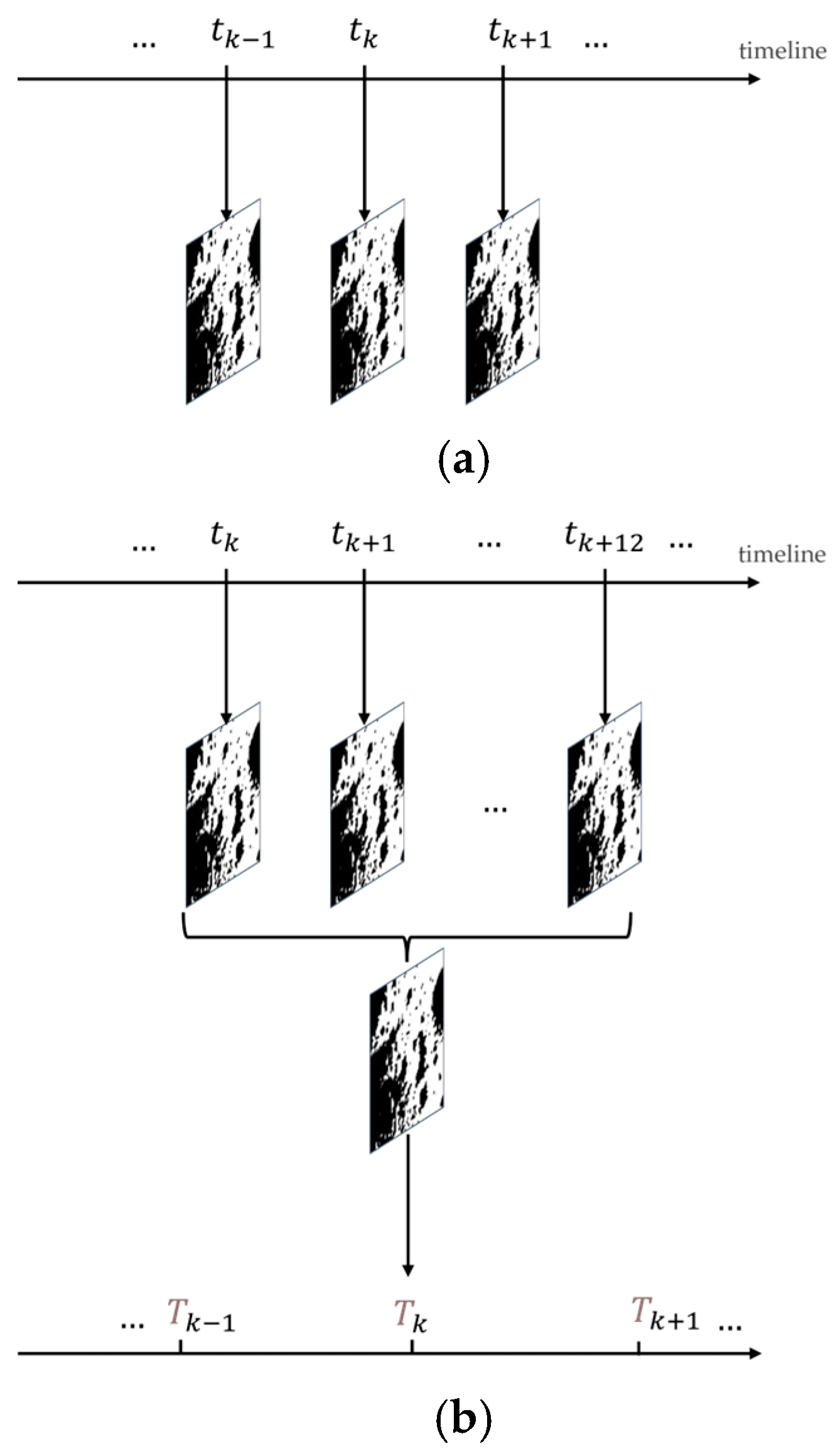
Figure 1. (a) Example of time-slice data; (b) Example of time-series data.
Remotesensing 17 01589 g001
Figure 2. Topography of the Moon’s south pole and sun visibility: (a) shows the DEM of the lunar south pole, oriented at 89°S, with the symbol “sp” marking the south pole and a square indicating the ROI; (b) presents the DEM for the ROI; (c) illustrates the time-averaged Sun visibility.
Remotesensing 17 01589 g002
Figure 3. Workflow of data generation.
Remotesensing 17 01589 g003
Figure 4. The architecture of the data preprocessing pipeline.
Remotesensing 17 01589 g004
Figure 5. Architecture of 3STU-Net-1 for time-slice 2.5D data.
Remotesensing 17 01589 g005
Figure 6. Architecture of 3STU-Net-2 for time-series 2.5D data.
Remotesensing 17 01589 g006
Figure 7. This is a figure to show the meanings of the characters in Formula (23).
Remotesensing 17 01589 g007
Figure 8. (a) Start node a (the green point) and goal node b (the red point); (b) Start node c (the green dot) and goal node d (the red dot). All data have the same ROI in Figure 2.
Remotesensing 17 01589 g008
Figure 9. History of Loss Function for the 3STU-Net, U-Net, and Attention U-Net.
Remotesensing 17 01589 g009
Figure 10. History of accuracy for the 3STU-Net, U-Net, and Attention U-Net.
Remotesensing 17 01589 g010
Figure 11. History of m I o U for the 3STU-Net, U-Net, and Attention U-Net.
Remotesensing 17 01589 g011
Figure 12. Comparison of selected results for 3STU-Net-1, U-Net, and Attention U-Net. All data have the same ROI in Figure 2. The red squares show the excellent performance of 3STU-Net-1 in the extraction of friendly-illumination areas.
Remotesensing 17 01589 g012
Figure 13. Comparison of selected results for 3STU-Net-2, U-Net, and Attention U-Net: (al) represent the 12 time-slice data that consist of the input time-series data for the 3STU-Net-2. The mean of (al) time-slice data was used as the input for U-Net and Attention U-Net. All data have the same ROI in Figure 2. The red square shows the excellent performance of 3STU-Net-2 in the extraction of friendly-illumination areas.
Remotesensing 17 01589 g013aRemotesensing 17 01589 g013bRemotesensing 17 01589 g013c
Figure 14. Path-planning results in different scenarios. All data have the same ROI in Figure 2. The green dot and the red dot denote the start node and the goal node, respectively, while the blue line illustrates the planned path.
Remotesensing 17 01589 g014aRemotesensing 17 01589 g014b
Figure 15. Path-planning results for scenario No. 4 of 3ST-A* with model preprocessed time-slice data in different time steps, n s = a ,   n g = b . All data have the same ROI in Figure 2. The green dot and the red dot denote the start node and the goal node, respectively, while the blue line illustrates the planned path.
Remotesensing 17 01589 g015aRemotesensing 17 01589 g015b
Table 1. The implementation process of the 3ST-A* algorithm.
1.Initialization
Input: Region slope S s l o p e , Region illumination F t k / F T k , Start node n s , Goal node n g , Current node n i , Current node slope s n i , Current node illumination f n i , t k / f n i , T k , Next chosen node illumination f n j , t k + 1 / f n j , T k + 1
Initialization: O p e n S e t = n s ,   C l o s e d S e t = ,   h n s = d i s n s , n g + h s l o p e ( n s ) + h i l l ( n s , f n s , t 0 ) / h i l l ( n s , f n s , T 0 ) ,     g n s = 0
2.Node Search and Path Planning
While True
 If n i is n g
  Add n i into C l o s e d S e t
  Break and return planning path C l o s e d S e t
 If f n i , t k / f n i , T k is not dark
  Add n i into C l o s e d S e t
 Else
  Rechoose a new non-dark node
 Set O p e n S e t =
 For each neighbor n e of neighbors at n i
   g ( n e ) = g ( n i ) + d i s n i , n e
   h ( n e ) = d i s n e , n g + h s l o p e ( n e ) + h i l l ( n e , f n e , t k ) / h i l l ( n e , f n e , T k )
   f n e = g n e + h ( n e )
  Add ( f n e , n e ) into O p e n S e t
 If O p e n S e t is empty
  Region illumination F t k / F T k F t k + 1 / F T k + 1
   f n i , t k / f n i , T k f n i , t k + 1 / f n i , T k + 1
  Stay, continue and begin the next iteration
n i a r g m i n   f n e     w h e r e   ( f n e   , n e ) O p e n S e t
 Region illumination F t k / F T k F t k + 1 / F T k + 1
f n i , t k / f n i , T k f n j , t k + 1 / f n j , T k + 1
3.End
Table 2. Illumination and Slope grid condition assessment.
Illumination Grid Condition Assessment
DarkWeakBright
SVF
Value Range
f n i , t k + 1 / f n i , T k + 1 0 0 < f n i , t k + 1 / f n i , T k + 1 0 .75 f n i , t k + 1 / f n i , T k + 1 > 0.75
Slope Grid Condition Assessment
ForbiddenGood
Slope
Value Range
s n i 20 ° s n i < 20 °
Table 3. Hyperparameters for 3STU-Net.
HyperparameterValues
Learning Rate1 × 10−4
OptimizerAdam
Batch Size8
Epochs30~800
α 0.3
ϵ 1 × 10⁻⁶
Table 4. Experiment setting.
No. n s n g A*3ST-A*Data Preprocessed Pipeline
Time-Slice Data3STU-Net-1 PreprocessedTim-Series Data3STU-Net-2 Preprocessed
1 a b
2 a b
3 a b
4 a b
5 a b
6 a b
7 c d
8 c d
9 c d
10 c d
Table 5. Extraction evaluation values of 3STU-Net-1, 3STU-Net-2, U-Net, and Attention U-Net.
Time-Slice DatasetTime-Series Dataset
(Time-Series Data Input)
Time-Series Dataset
(Mean Data Input)
Accuracy m I o U Accuracy m I o U Accuracy m I o U
3STU-Net-195.0187.18----
3STU-Net-2--96.4391.83--
U-Net94.8986.87--94.9989.94
Attention U-Net94.8086.67--94.9089.75
Table 6. Experiment result for path planning in different scenarios.
No. n s n g AG 1SG 2Total StepsPlanning Time
(s)
NoINoSStay
DarkWeakBrightForbiddenGood
1abA*-1042320236101040
2abA*-1042424196101040
3ab3ST-A*-1473405387 + 7R 301471
4ab3ST-A*3STU-Net-15221190052205220
5ab3ST-A*-1482706180 + 7R014828
6ab3ST-A*3STU-Net-25081260050805080
7cd3ST-A*-621103590620
8cd3ST-A*3STU-Net-1621600620620
9cd3ST-A*-621104580620
10cd3ST-A*3STU-Net-2621400620620
1 AG: Algorithm. 2 SG: Segmentation operation model. 3 R: Rechoosing a new non-dark node.
Disclaimer/Publisher’s Note: The statements, opinions and data contained in all publications are solely those of the individual author(s) and contributor(s) and not of MDPI and/or the editor(s). MDPI and/or the editor(s) disclaim responsibility for any injury to people or property resulting from any ideas, methods, instructions or products referred to in the content.