A VMD-SVM Method for LEO Satellite Orbit Prediction with Space Weather Parameters

Abstract

The technology of satellite orbit prediction (OP) is crucial in space engineering. However, it is difficult to precisely predict medium and long-term orbit for the low Earth-orbit (LEO) satellites because of time-varying space weather and inaccurate atmospheric density models. To address the problem, a novel intelligent OP method based on the variational mode decomposition-support vector machine (VMD-SVM) framework is presented. First, the concept of a pseudo-drag coefficient is defined, transforming the OP problem into a pseudo-drag coefficient prediction problem. Second, the relationship between space weather parameters and the pseudo-drag coefficient is analyzed using the VMD method, from which a strong correlation is shown. Furthermore, an SVM model combined with space weather characteristic parameters is employed to predict the pseudo-drag coefficient, significantly improving the precision of OP when further integrated into the orbital dynamics model. Experiments with data from engineering applications show that VMD-SVM medium and long-term OP technology is practical and effective.

1. Introduction

With the rapid development of space technology, an increasing number of satellite are being deployed into orbit. Therefore, highly accurate and precise orbit prediction (OP) has become crucial in space engineering applications [1,2]. Orbit information for the satellite is obtained via orbit determination (OD) and OP processes [3]. The OD process uses observation data to estimate accurate historical orbit data and other parameters, such as the atmospheric drag coefficient. However, in the OP process, observation data are not available, and the accuracy of future orbit data depends on the orbital initial state and orbital dynamic model [4]. For LEO satellites, although conservative forces, including the earth gravity force and third-body perturbations, can be well modeled, non-conservative perturbations, such as atmospheric drag, may have higher uncertainty, which is manifested in the complexity of atmospheric density modeling and the stochastic nature of space weather [5,6,7].

Currently, in order to improve the OP accuracy of LEO satellites, many scholars have made significant contributions to the field of machine learning (ML). A significant consideration is the understanding of error rules for orbit propagation processes by supervised learning, aimed at compensating for the inherent inaccuracies in the results produced by orbit propagation processes. Peng et al. used a support vector machine (SVM), Gaussian process, and artificial neural network, respectively, to enhance OP accuracy, showing that ML models are effective in this respect [8,9,10,11]. Similarly, Li et al. established a true orbital dataset with two-line element (TLE) entries and studied the convolutional neural network (CNN) and the gradient boosting decision tree (GBDT) to model the rules of OP errors [12]. Zhai et al. utilized a principal component analysis–extreme gradient boosting (PCA-XGBoost) model for experiments in a simulation environment [13]. Huang et al. used an XGBoost-based method for improved orbit prediction with an orbit-separate modeling strategy [14]. Furthermore, Peng et al. recently enhanced the precision of OP via the integration of filtering algorithms and ML techniques [15,16]. Haidar et al. proposed a hybrid analysis method utilizing ML for the OP of LEO satellites [17]. The preceding research shows the considerable potential of ML in the domain of OP, offering a valuable reference point.

Most current research employs ML to model the error rule of orbit propagation, thereby enhancing the precision of OP. It is typically based on the premise that the error in orbit propagation follows a certain pattern, such as upward fluctuations in error magnitude [12,14]. However, the fluctuation direction of the OP error depends on the difference between the predicted and actual atmospheric drag. In practice, it is challenging to make precise predictions about real space weather variations. Consequently, when making medium and long-term OP, it is not always possible to determine the direction in which the prediction error will fluctuate.

In this paper, atmospheric drag is used as a research entry point, as it is the principal factor influencing OP for LEO satellites. Extensive research has shown that the correction of the atmospheric drag model can enhance the accuracy of OP [18,19,20,21]. There are two primary research focuses: the first is the estimation of the atmospheric density model, for which existing methods include those based on orbit derivations [22,23], various empirical models using accelerometers [24,25,26], and global navigation satellite system (GNSS) data [27,28]. In recent years, ML methods have been employed in studies aimed at correcting the atmospheric density model [29,30,31]. The other focus is the analysis of the atmospheric drag coefficient. Wang et al. demonstrated that modifying the drag modulation coefficient of the SGP model can decrease the along-track error [32]. Similarly, there are also related applications in the domain of ML. Cimmino et al. proposed a ballistic coefficient estimation method using ML [33], while Paul et al. employed ML technology to model the satellite drag coefficient and quantify the orbit propagation uncertainty [34].

In view of the above, to address the problem of medium and long-term OP for LEO satellites, an intelligent OP method using VMD-SVM is proposed. The main contributions are as follows:

(1)

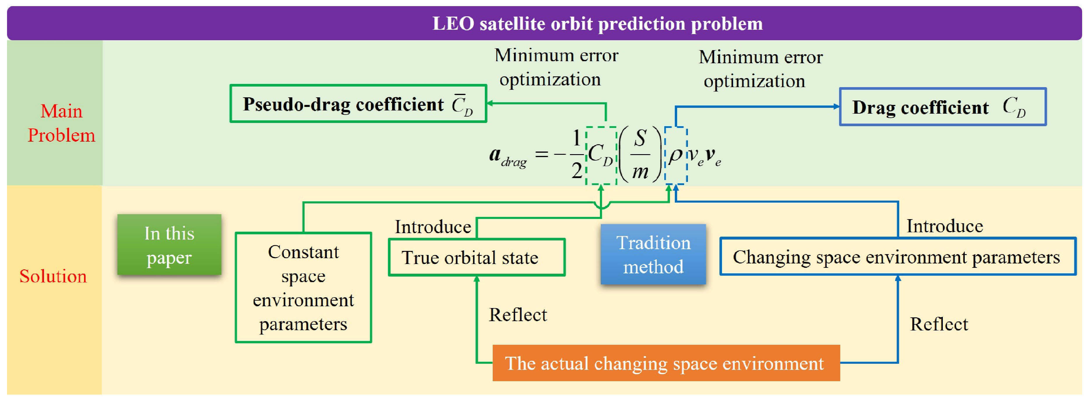
The concept of the pseudo-drag coefficient is defined, relating space weather to the atmospheric drag model and transforming the OP problem of LEO satellites into a pseudo-drag coefficient prediction problem.

(2)

The correlation between space weather parameters and the pseudo-drag coefficient is analyzed using the VMD method, which shows a strong correlation. Additionally, the space weather feature variables required for ML input can be derived from this analysis.

(3)

The prediction model for the pseudo-drag coefficient is established using ML, and it can improve the precision of OP when integrated into the orbital dynamics model.

In Section 2, we analyze the key problems of LEO satellite OP and propose solutions. Section 3 explores the relationship between space weather parameters and the pseudo-drag coefficient. Section 4 introduces an intelligent OP method. Section 5 presents the experimental results. Finally, the paper is summarized in Section 6.

Notations: The symbol $C_D$ represents the drag coefficient, estimated using the traditional OD method, and is used for traditional OP. ${\overline{C}}_D$ denotes the pseudo-drag coefficient, which is the target variable of the machine learning model and is used for intelligent OP. ${\widehat{C}}_D$ denotes the equivalent drag coefficient, which is the feature variable of the machine learning model and is used for equivalent traditional OP under the same space weather conditions as the ${\overline{C}}_D$.

2. The LEO Satellite OP Problem and Method

2.1. Description and Analysis of the Problem

Currently, for LEO satellites, the approach for OP in the field of engineering is the OD/OP framework. The OD process is employed to obtain accurate orbit state vectors as an estimation of the true orbit. Subsequently, the state vectors serve as initial values for the OP process, which utilizes the same physical model used in the OD process for prediction. In this paper, the OD/OP framework is referred to as the traditional method. It is well known that in this method, the perturbation model of the conservative forces can be well modeled, and the main source of uncertainty in the dynamic model is the atmospheric drag in non-conservative forces.

For a satellite of mass m, the acceleration formula caused by atmospheric drag is as follows:

$${\mathit{a}}_{drag}=-{\displaystyle \frac{1}{2}}\left({\displaystyle \frac{S}{m}}\right)C_D\rho v_e{\mathit{v}}_e,$$

(1)

where $C_D$ is the atmospheric drag coefficient, ${\displaystyle \frac{S}{m}}$ is the area-to-mass ratio, $\rho$ is the atmospheric density, which is related to orbital altitude, ${\mathit{v}}_e$ is the velocity vector of the spacecraft relative to the atmosphere, and $v_e={∥{\mathit{v}}_e∥}_2$, ${∥.∥}_2$ represents the Euclidean norm.

All variables on the right side of Equation (1) are uncertain, and most scholars focus on $\rho$ and $C_D$ among these variables. $\rho$ is usually estimated by atmospheric empirical models, such as NRLMSIS-00, DTM2000, and JB2008. $C_D$ is often utilized as the state vector for the spacecraft, with estimates derived during the OD process to absorb the error of the atmospheric drag model. The formula for calculating the derivative of atmospheric drag perturbation to $C_D$ is as follows:

$${\displaystyle \frac{\partial {\mathit{a}}_{drag}}{\partial C_D}}=-{\displaystyle \frac{1}{2}}\left({\displaystyle \frac{S}{m}}\right)\rho v_e{\mathit{v}}_e.$$

(2)

It is widely acknowledged that changes in space weather have a direct impact on the estimation of atmospheric density $\rho$. As illustrated in Equations (1) and (2), this will also impact the solution of $C_D$. Therefore, the drag coefficient depends on atmospheric density, meaning the estimated drag coefficient during orbit determination is self-consistent with contemporaneous space weather conditions. However, this coefficient may not be suitable for the OP phase, especially in medium and long-term OP.

In the traditional method, the accuracy of OP is influenced by atmospheric drag, which, in turn, relies on the precision of space weather forecasts. However, accurate space weather forecasting is still a difficult problem. Therefore, during short-term OP or when space weather is stable, the traditional method will achieve good results. Under either medium and long-term OP or notable changes in space weather, the atmospheric density $\rho$ is difficult to accurately estimate, and the $C_D$ value calculated in the OD process cannot be adapted to the error absorption in the OP process, resulting in prediction errors increasing rapidly.

2.2. Method

In this section, the motivation for the proposed VMD-SVM method is provided to highlight the significance of LEO satellite OP. Then, the concept of the pseudo-drag coefficient is defined, and the main framework is introduced. Among them, the precise ephemeris is generated using GNSS observation data combined with orbit determination methods and is used as the true value of the orbit in the paper. Following the main framework, the key components of the VMD-SVM method are described.

2.2.1. Motivation

Accurate OP of LEO satellites is essential for space engineering, compelling us to consider effective strategies to achieve this objective. Uncertainty in estimating atmospheric density is the primary source of OP errors. Additionally, the adaptability of the atmospheric drag coefficient will also affect the error absorption, both of which are closely related to the change in space weather. A possible solution is to improve the atmospheric drag model by using space weather data, but there are still several inherent difficulties: (1) what parameters are used to establish the relationship between space weather and the atmospheric drag model, (2) how do we describe this relationship, and (3) how do we model this relationship?

2.2.2. VMD-SVM Framework

In view of the above three difficulties, a new VMD-SVM method is proposed to address the OP problem of LEO satellites in practical engineering. The overall framework of the method is illustrated in Figure 1 and consists of three main components: the concept and solution of the pseudo-drag coefficient, the analysis of the relationship between space weather parameters and the pseudo-drag coefficient, and training and prediction using the ML model.

First, the pseudo-drag coefficient is solved using the golden section method, transforming the OP problem into a pseudo-drag coefficient prediction problem. Second, the relationship between space weather and the pseudo-drag coefficient is analyzed using VMD technology. Furthermore, the SVM regression method, an advanced technique proven to be robust against outliers in the dataset, especially in small sample scenarios, is chosen in this paper. Nevertheless, the proposed framework is expected to be general and applicable to other ML methods. Finally, the overall framework introduces and embeds a learning-centered strategy into the orbital dynamics model to achieve accurate OP.

3. VMD-Based Analysis of Space Weather and the Pseudo-Drag Coefficient

3.1. Concept of the Pseudo-Drag Coefficient

• Concept

The core challenge in LEO satellite OP lies in the accuracy of the atmospheric drag model, with the inability to accurately model space weather variations being the main factor affecting the precision of the drag model. Traditional methods face two problems in medium and long-term OP: on the one hand, errors in predicting space weather parameters (such as solar radiation index and geomagnetic activity index) propagate through atmospheric density calculations and affect the orbit model; on the other hand, the drag coefficient $C_D$ estimated during the OD phase is challenging to adapt to the space environment in the OP phase. The coupling effect of these two sources of uncertainty limits the reliability of traditional methods in medium and long-term LEO satellite OP.

To address this issue, this paper proposes the concept of the “pseudo-drag coefficient ${\overline{C}}_D$”. Based on the relationship where atmospheric drag is proportional to both atmospheric density and the drag coefficient, the uncertainty in space weather prediction and the adaptation of traditional $C_D$ parameters are unified into a single adjustment term, the “pseudo-drag coefficient ${\overline{C}}_D$”. Changes in the space environment can not only be characterized by accurate space weather parameters but will ultimately be reflected in the true orbital state of the satellite. Using true orbital data as a reference, atmospheric density is calculated by adopting fixed space environment parameters, and the drag coefficient is adjusted to achieve the best match between the predicted and true orbits. In this case, the drag coefficient, which contains the effects of space weather on the orbit, is defined as the pseudo-drag coefficient ${\overline{C}}_D$, as shown in Figure 2.

By constructing a time series dataset of the pseudo-drag coefficient using historical orbital data and using machine learning methods to explore the implicit mapping relationship between the pseudo-drag coefficient and space environment parameters, the orbit prediction problem is transformed into a prediction problem of the pseudo-drag coefficient.

B.

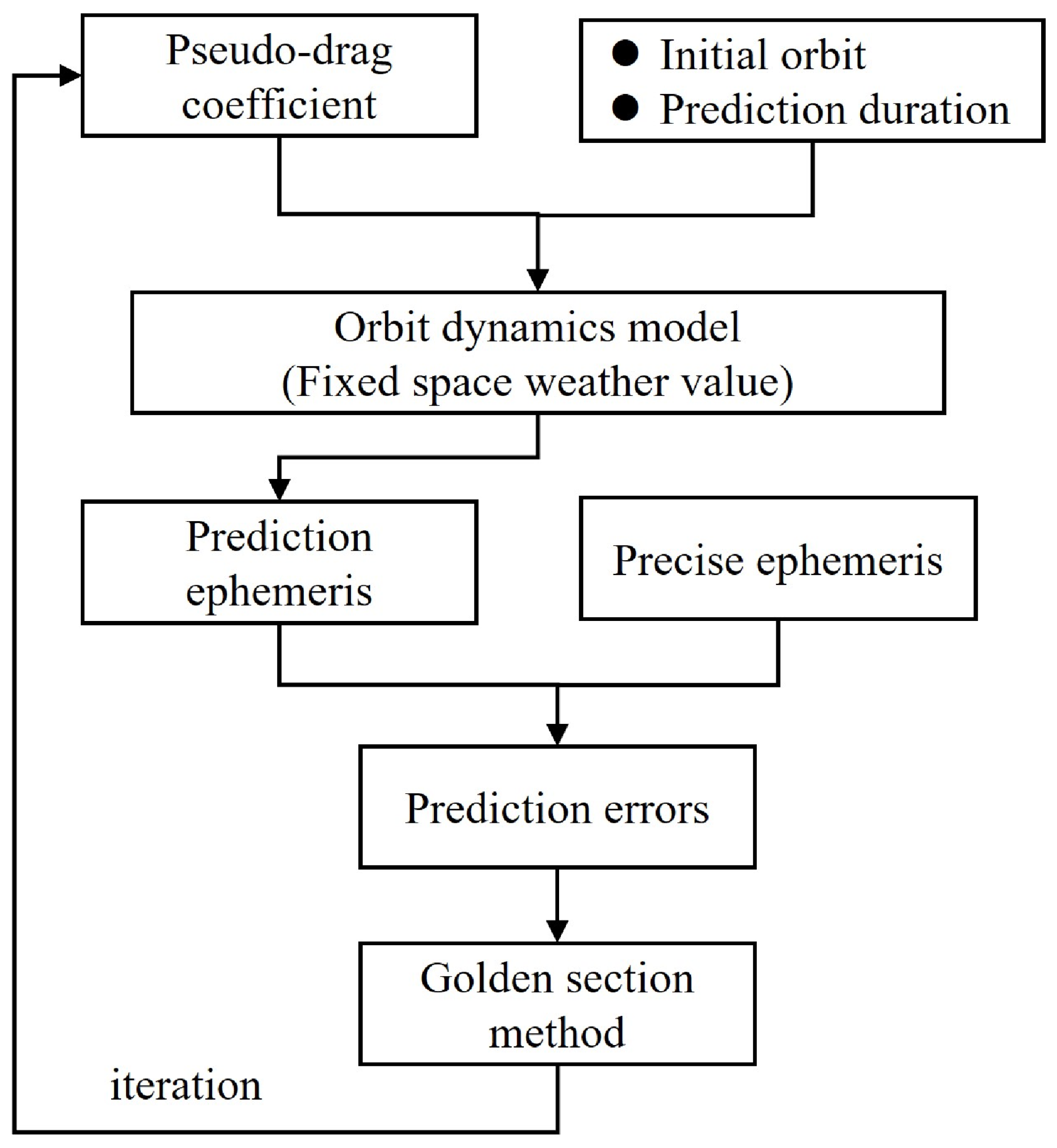
Compute

The solution of ${\overline{C}}_D$ requires the true satellite orbit and a high-precision orbit dynamics model. In this paper, the true satellite orbit is approximately replaced using observation data of the satellite, referred to as precise ephemeris data. The orbit dynamics model is provided by the following:

$$\left\{\begin{array}{l}\ddot{\mathit{r}}=-\mu {\displaystyle \frac{\mathit{r}}{r^3}}+{\mathit{a}}_p\\ {\mathit{a}}_p={\mathit{a}}_{harmonic}+{\mathit{a}}_{third-body}+{\mathit{a}}_{drag}+{\mathit{a}}_{SRP}+{\mathit{a}}_{other}\end{array},\right.$$

(3)

where $\mathit{r}$ and $\dot{\mathit{r}}$ represent the position and velocity vector, respectively. $r={∥\mathit{r}∥}_2$, ${∥.∥}_2$ represents the Euclidean norm, $\ddot{\mathit{r}}$ represents the second derivative of the vector $\mathit{r}$, $\mu$ is the gravitational parameter of the earth, and ${\mathit{a}}_p$ is the perturbation acceleration vector caused by the non-spherical gravity, three-body gravity attraction, atmospheric drag, solar radiation pressure, and other (tidal and relativistic effect). In addition to the atmospheric drag perturbation, other perturbation models can be well modeled or have little effect on LEO satellites.

In the traditional method, the inputs of the atmospheric drag model include the geomagnetic index and solar radio flux index, and changes in space weather are reflected in the atmospheric density. In this paper, the geomagnetic index and solar radio flux index are set as fixed values. Given the initial epoch $t_0$ and the initial orbital state ${\mathit{x}}_{\mathbf{0}}={[\mathit{r},\dot{\mathit{r}}]}_{t=t_0}$, along with the pseudo-drag coefficient ${\overline{C}}_D$, the orbit state at any future epoch t can be regarded as a single-variable function of the pseudo-drag coefficient, as shown in Equation (4).

$${\mathit{x}}_{{\overline{C}}_D}(t,t_0,{\overline{C}}_D)=f(t,t_0,{\mathit{x}}_0,{\overline{C}}_D),$$

(4)

where ${\mathit{x}}_{{\overline{C}}_D}(t,t_0,{\overline{C}}_D)$ is the state prediction at t, $t>t_0$. $f\left(•\right)$ is the state solution of Equation (3), which can be solved by a numerical orbit propagator.

Utilizing the principle of minimizing prediction errors between precise ephemeris data and predicted ephemeris, when the $\mathcal{F}\left({\overline{C}}_D\right)$ in Equation (5) reaches its minimum value, ${\overline{C}}_D$ is determined as the unique optimization variable, representing the pseudo-drag coefficient.

$$\left\{\begin{array}{c}\mathcal{F}\left({\overline{C}}_D\right)={\displaystyle \sum _{k=1}^N}{∥{\mathit{x}}_{{\overline{C}}_D}(t_k,t_0,{\overline{C}}_D)-{\mathit{x}}_{\mathrm{true}}\left(t_k\right)∥}_2\hfill \\ {\displaystyle \underset{{\overline{C}}_D\in S}{min}}\mathcal{F}\left({\overline{C}}_D\right),S={\mathbb{R}}^{+}\hfill \end{array},\right.$$

(5)

where $\mathcal{F}\left({\overline{C}}_D\right)$ is the cost function, ${\mathit{x}}_{\mathrm{true}}\left(t_k\right)$ represents the precise ephemeris data at time $t_k$, obtained through the OD process using satellite observation data, and N is the number of data points.

The solution of the ${\overline{C}}_D$ sequence can be explained as an optimization problem involving a univariate function. The golden section search is a method for determining the extreme value of a function by searching within a known interval using the golden ratio. It is relatively simple, does not require derivative information, and demonstrates good convergence during the iterative process. Therefore, in this paper, the ${\overline{C}}_D$ sequence is obtained using the golden section method, and the specific solution process is shown in Figure 3.

C.

Validate

It can be seen from the solution process of the ${\overline{C}}_D$ that its solution is related to the prediction time. This paper focuses on improving the medium and long-term OP for LEO satellites. Considering the engineering application, a prediction period of 10 days is selected. In addition, inspired by the approach of solving the ${\overline{C}}_D$, as a comparison, the OP ephemeris of the traditional method can be used to replace the role of the precise ephemeris in the ${\overline{C}}_D$ solution process, and the equivalent-drag coefficient ${\widehat{C}}_D$ under the same conditions can be obtained. The ${\widehat{C}}_D$ can be used to characterize the OP accuracy of the traditional method, while the ${\overline{C}}_D$ can be used to characterize the OP accuracy of the proposed method, which also represents the better OP result under the current conditions.

Taking the LEO satellite SAT1 as an example, we use observation data from a satellite with an orbital altitude of approximately 400 km. Under the same conditions, OP was completed using ${\overline{C}}_D$, ${\widehat{C}}_D$, and the traditional method, respectively. The OP errors in the RAC coordinate system are shown in Figure 4a–c. The improvement effect of the ${\overline{C}}_D$ prediction method and the ${\widehat{C}}_D$ prediction method, compared to the traditional prediction method, is shown in Figure 4d. To compare the OP errors, consistent scaling is applied while preserving the differences and proportions within the error data. The scaling principle takes the maximum prediction error of ${\overline{C}}_D$ as the unit, and the scaled error $Enor{m}_i\left(t\right)$ is shown as follows:

$$Enor{m}_i\left(t\right)={\displaystyle \frac{Eothe{r}_i\left(t\right)}{max\left|Epc{d}_i\left(t\right)\right|}},$$

(6)

where $Epc{d}_i\left(t\right)$ represents OP errors when selecting the ${\overline{C}}_D$, $Eothe{r}_i\left(t\right)$ represents OP errors of ${\widehat{C}}_D$ and the traditional method, and $i\in \left\{R,A,C\right\}$ represents the radial, along-track, and cross-track errors, respectively.

The following conclusions are shown in Figure 4:

(1)

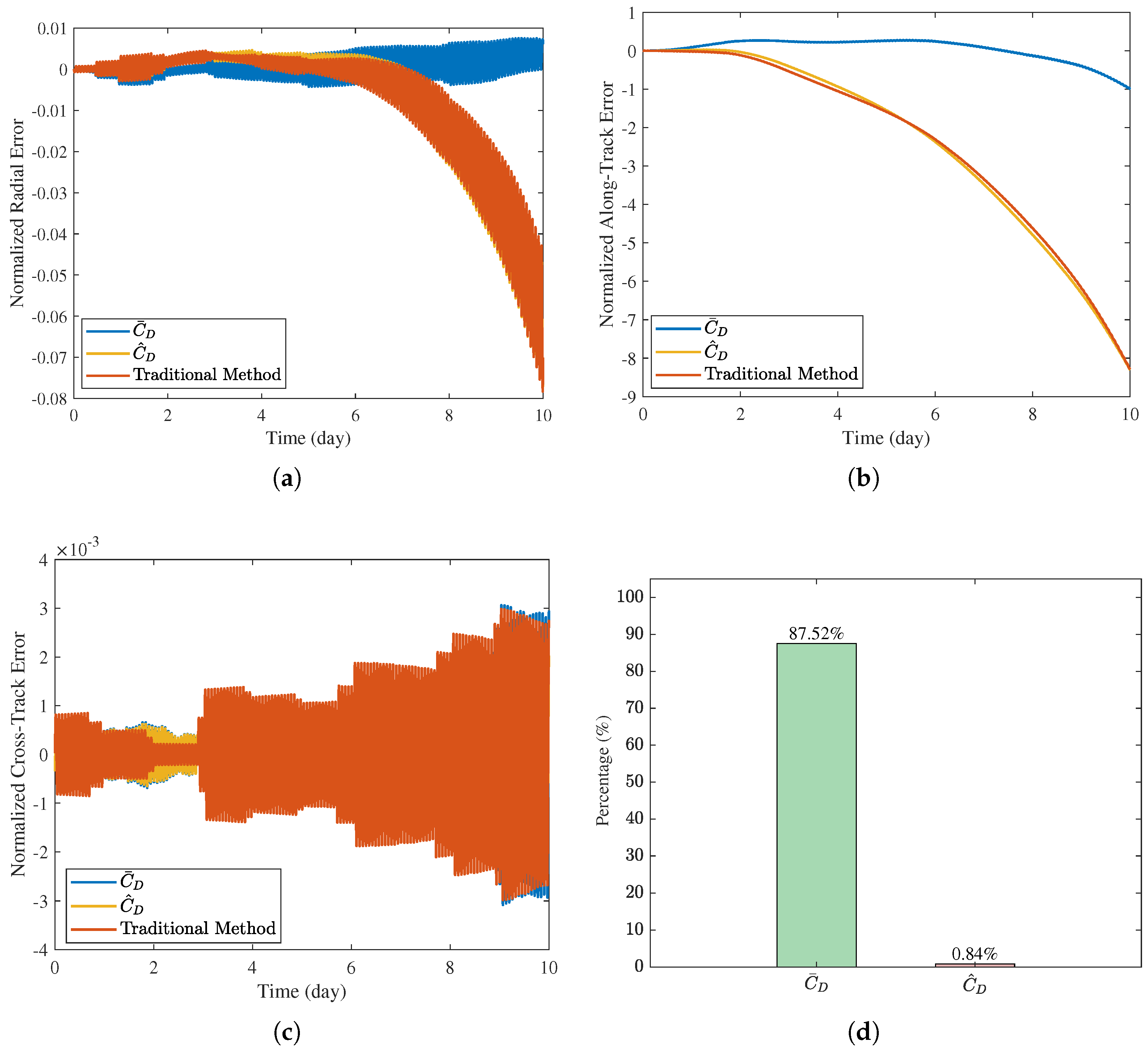
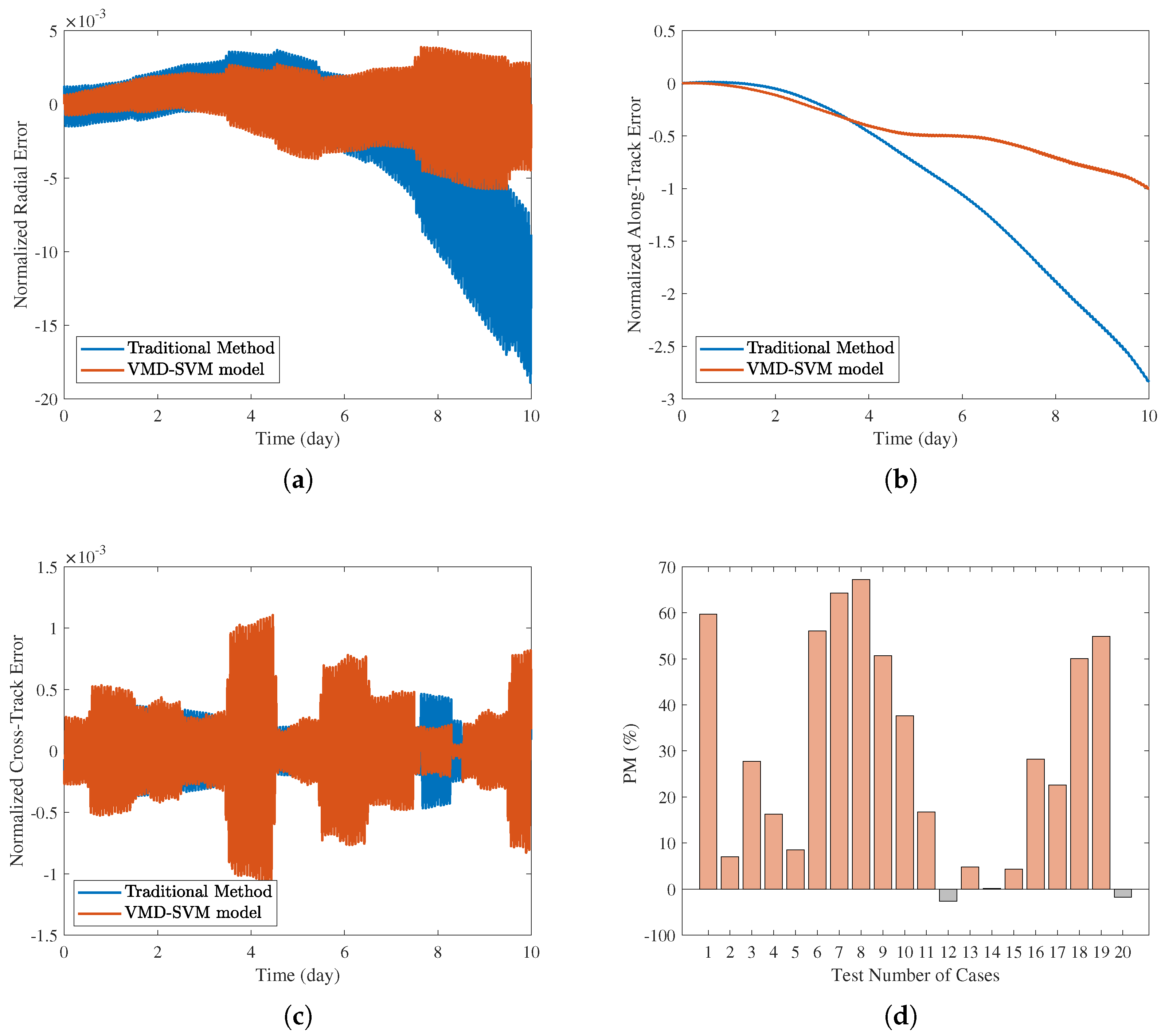
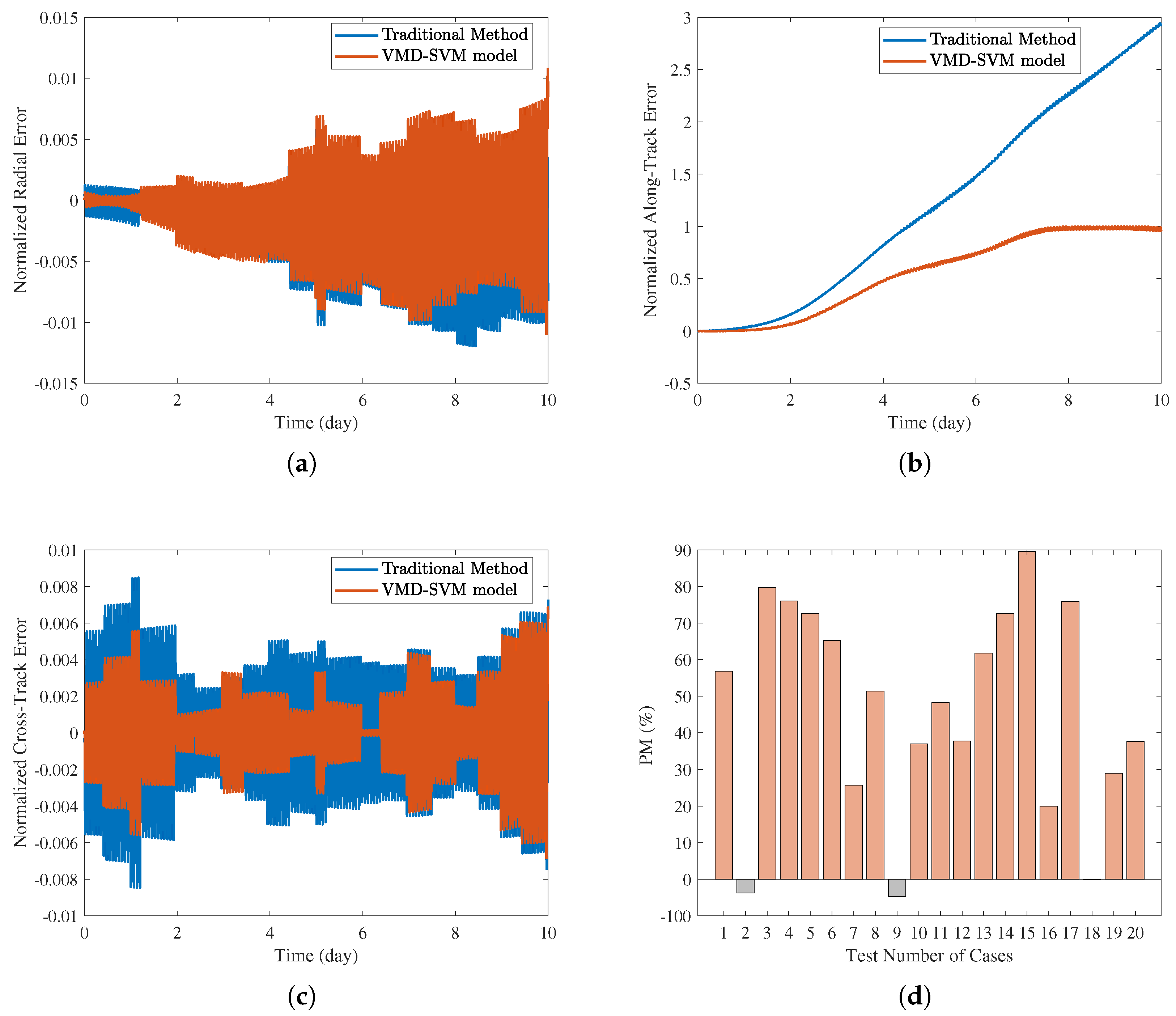
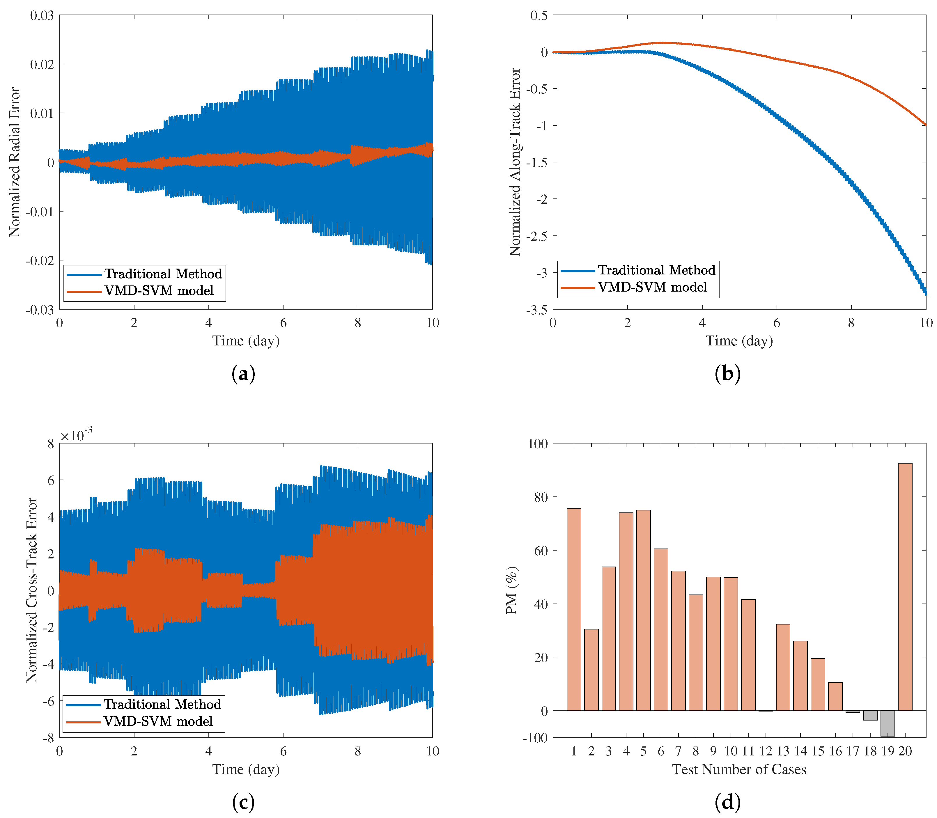
The OP error of the LEO satellite is mainly in the along-track direction, the error being significantly greater in magnitude than that in the radial and cross-track directions.

(2)

${\overline{C}}_D$ can effectively absorb OP errors, which primarily affect the along-track error. The radial error is much smaller than the along-track error but can still be improved, while the cross-track error has little effect.

(3)

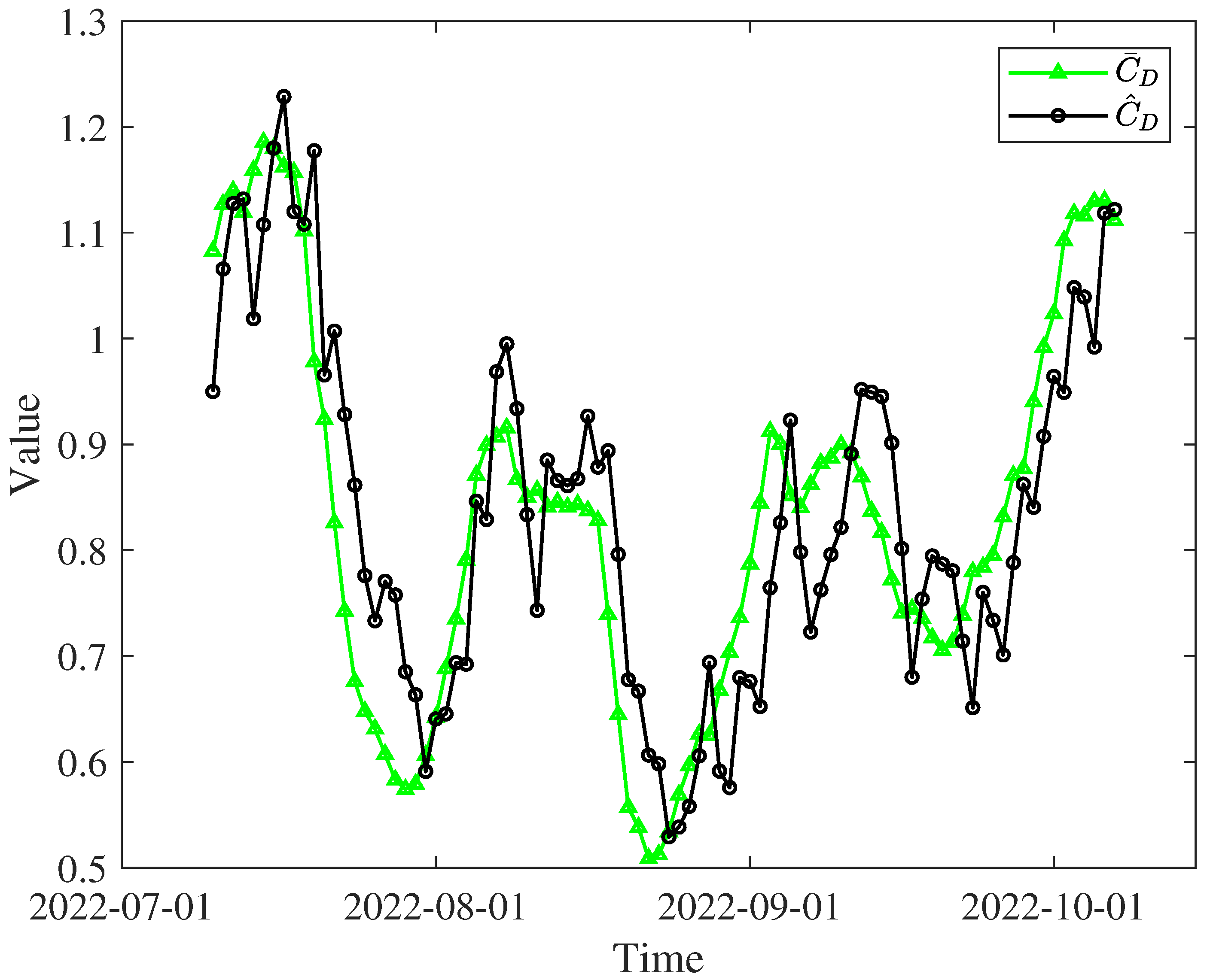
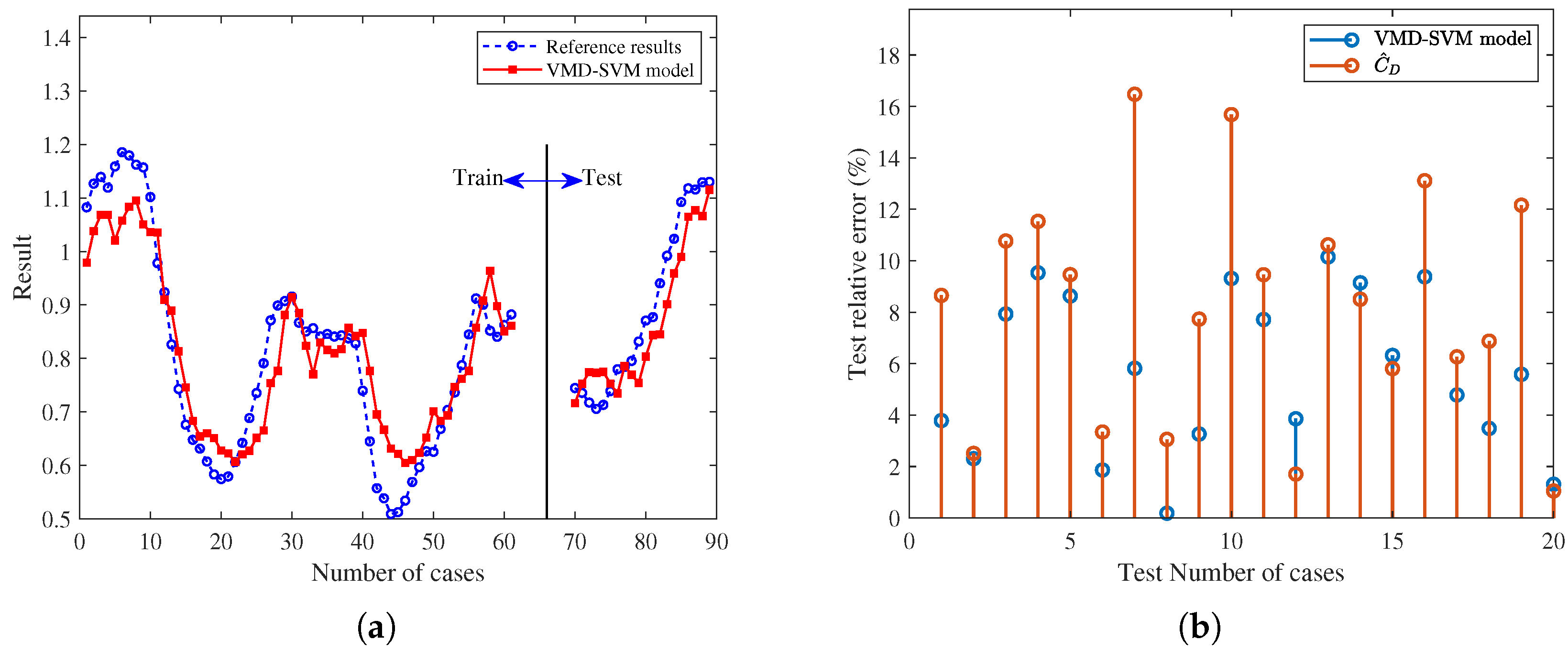
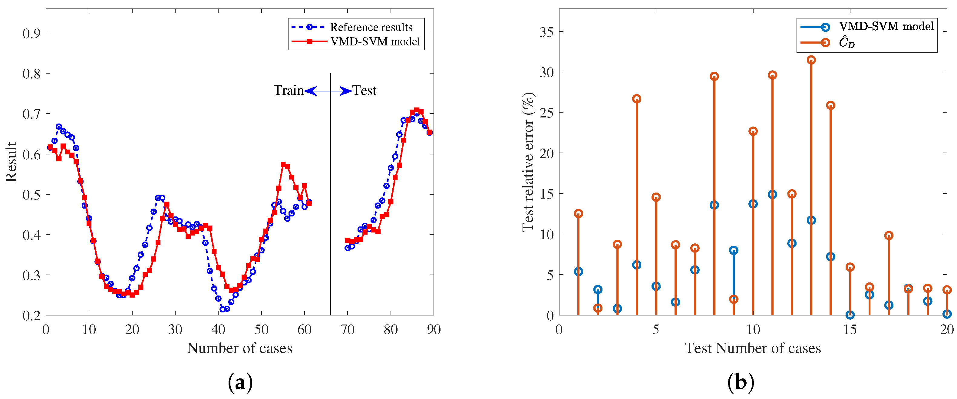
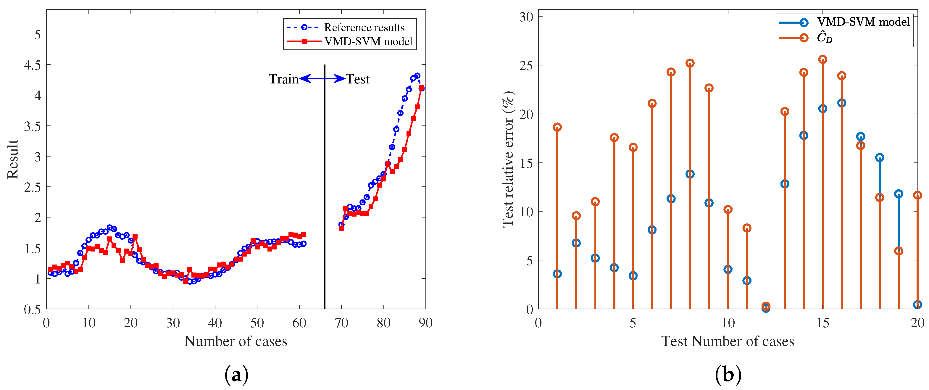
The prediction of the ${\widehat{C}}_D$ can approximately represent the results of the traditional method.

Furthermore, from 10 July 2022 to 17 October 2022, the ${\overline{C}}_D$ and ${\widehat{C}}_D$ were solved using the precise ephemeris of the SAT1 satellite, as shown in Figure 5. Figure 6 shows the error rate of the ${\widehat{C}}_D$ relative to the ${\overline{C}}_D$, which can be expressed as follows.

$$R=\left|{\displaystyle \frac{{\widehat{C}}_D-{\overline{C}}_D}{{\overline{C}}_D}}\right|\times 100\%.$$

(7)

It can be seen from Figure 6 that the maximum error rate of ${\widehat{C}}_D$ relative to ${\overline{C}}_D$ can reach 30%, and there are a few error rates close to 0. This indicates that the traditional method shows a wide range of prediction error distribution and a large confidence interval in the 10-day OP. An error rate close to 0 indicates that the traditional method has a small absolute error in OP, which is consistent with the actual situation.

The pseudo-drag coefficient is highly significant, as it establishes a connection between space weather and the atmospheric drag model, addressing the first difficulty.

3.2. Data Preprocessing Using VMD

Variational mode decomposition (VMD) is an adaptive signal decomposition method that effectively deals with non-stationary and nonlinear signals [35]. The construction of the VMD involves Wiener filtering, the Hilbert transform, and frequency mixing techniques. The frequency center and bandwidth of each subcomponent are determined by iteratively searching the optimal solution of the variational mode. In order to perform adaptive frequency domain separation of the signal, the model estimation is transformed into a variational problem. The VMD method utilizes a variational model during the decomposition process to identify a solution within a constraint variational model, thereby achieving a more advanced signal decomposition. The main mechanism of decomposition can be described as follows:

(1) Each intrinsic modulus function (IMF) component is defined as the non-smooth component, which can be expressed as

$$u_k\left(t\right)=A_k\left(t\right)cos\left({\varphi }_k\left(t\right)\right),$$

(8)

(2) The Hilbert transform is utilized on each IMF component, and then the unilateral spectrum is extracted.

$$\left[\begin{array}{c}\delta \left(t\right)+{\displaystyle \frac{j}{\pi t}}\end{array}\right]\ast u_k\left(t\right),$$

(9)

where * is the convolution operator, $\delta \left(t\right)$ is the Dirichlet function, and j is the imaginary part.

(3) For each IMF, the spectrum is modulated to the fundamental frequency band by mixing the exponential terms of its corresponding central frequency.

$$\left[\begin{array}{cc}\left[\begin{array}{c}\delta \left(t\right)+{\displaystyle \frac{j}{\pi t}}\end{array}\right]\ast & u_k\left(t\right)\end{array}\right]\begin{array}{c}{e}^{-j{\omega }_{k}t}\end{array},$$

(10)

where ${\omega }_k$ is the center frequency of $u_k\left(t\right)$.

(4) The Gaussian smoothing method of the demodulated signal is used to estimate the bandwidth of each IMF component to solve the constrained variational problem. The objective function is

$$\left\{\begin{array}{c}{min}_{\left\{u_k\right\},\left\{{\omega }_k\right\}}\left\{{\displaystyle \sum _{k=1}^K}{∥{\partial }_t\left\{\left[\delta \left(t\right)+{\displaystyle \frac{j}{\pi t}}\right]\ast u_k\left(t\right)\right\}·e^{-j{\omega }_{k}t}∥}_2^2\right\}\hfill \\ s.t.{\displaystyle \sum _{k=1}^K}{u}_k=f\left(t\right)\hfill \end{array},\right.$$

(11)

where, ${\partial }_t$ is the partial derivative, $\left\{u_k\right\}=\{u_1,\dots ,u_k\}$ and $\left\{{\omega }_k\right\}=\{{\omega }_1,\dots ,{\omega }_k\}$ are the modal component and the center frequency of the decomposition, respectively, and $f\left(t\right)$ is the original signal.

(5) By introducing the penalty factor $\alpha$ and the Lagrangian operator $\lambda \left(t\right)$, the unconstrained variational problem can be obtained from the constrained variational problem. The expression of the extended Lagrangian problem can be expressed as follows.

$$\begin{array}{c}L(\left\{u_k\right\},\left\{{\omega }_k\right\},\lambda )=\alpha {\displaystyle {\displaystyle \sum _k}}{∥{\partial }_t[(\delta \left(t\right)+j/\pi t)\ast u_k\left(t\right)]e^{-j{\omega }_{k}t}∥}_2^2+{∥f\left(t\right)-{\displaystyle \sum _k}{u}_k\left(t\right)∥}_2^2\hfill \\ +\langle \lambda \left(t\right),f\left(t\right)-{\displaystyle \sum _k}{u}_k\left(t\right)\rangle \hfill \end{array},$$

(12)

(6) In the iterative search process, the alternating direction multiplier method is used to solve Equation (10), and the optimal solution of the constrained variational model is obtained.

$$\begin{array}{c}\hfill {\widehat{u}}_k^{n+1}\leftarrow {\displaystyle \frac{\widehat{f}\left(\omega \right)-{\displaystyle \sum _{i\ne k}}{\widehat{u}}_i^{n+1}+\frac{{\widehat{\lambda }}^n\left(\omega \right)}{2}}{1+2\alpha {(\omega -{\omega }_k^n)}^2}}\end{array}$$

(13)

$$\begin{array}{c}\hfill {\widehat{\omega }}_k^{n+1}\leftarrow {\displaystyle \frac{{\int }_0^{\infty }\omega {\left|{\widehat{u}}_k^{n+1}\left(\omega \right)\right|}^2\mathrm{d}\omega }{{\int }_0^{\infty }{\left|{\widehat{u}}_k^{n+1}\left(\omega \right)\right|}^2\mathrm{d}\omega }}\end{array}$$

(14)

$$\begin{array}{c}\hfill {\widehat{\lambda }}^{n+1}\left(\omega \right)\leftarrow {\widehat{\lambda }}^n\left(\omega \right)+\tau \left(\widehat{f}\left(\omega \right)-{\displaystyle \sum _k}{\widehat{u}}_k^{n+1}\left(\omega \right)\right),\end{array}$$

(15)

where $\tau$ is noise tolerance.

The iterative process continues until the convergence is satisfied or the maximum allowable number of iterations is reached.

$${\displaystyle \frac{\Vert {\widehat{u}}_k^{n+1}-{\widehat{u}}_k^n{\Vert }_2^2}{\Vert {\widehat{u}}_k^n{\Vert }_2^2}}<\epsilon ,$$

(16)

where $\epsilon$ is the tolerance of convergence.

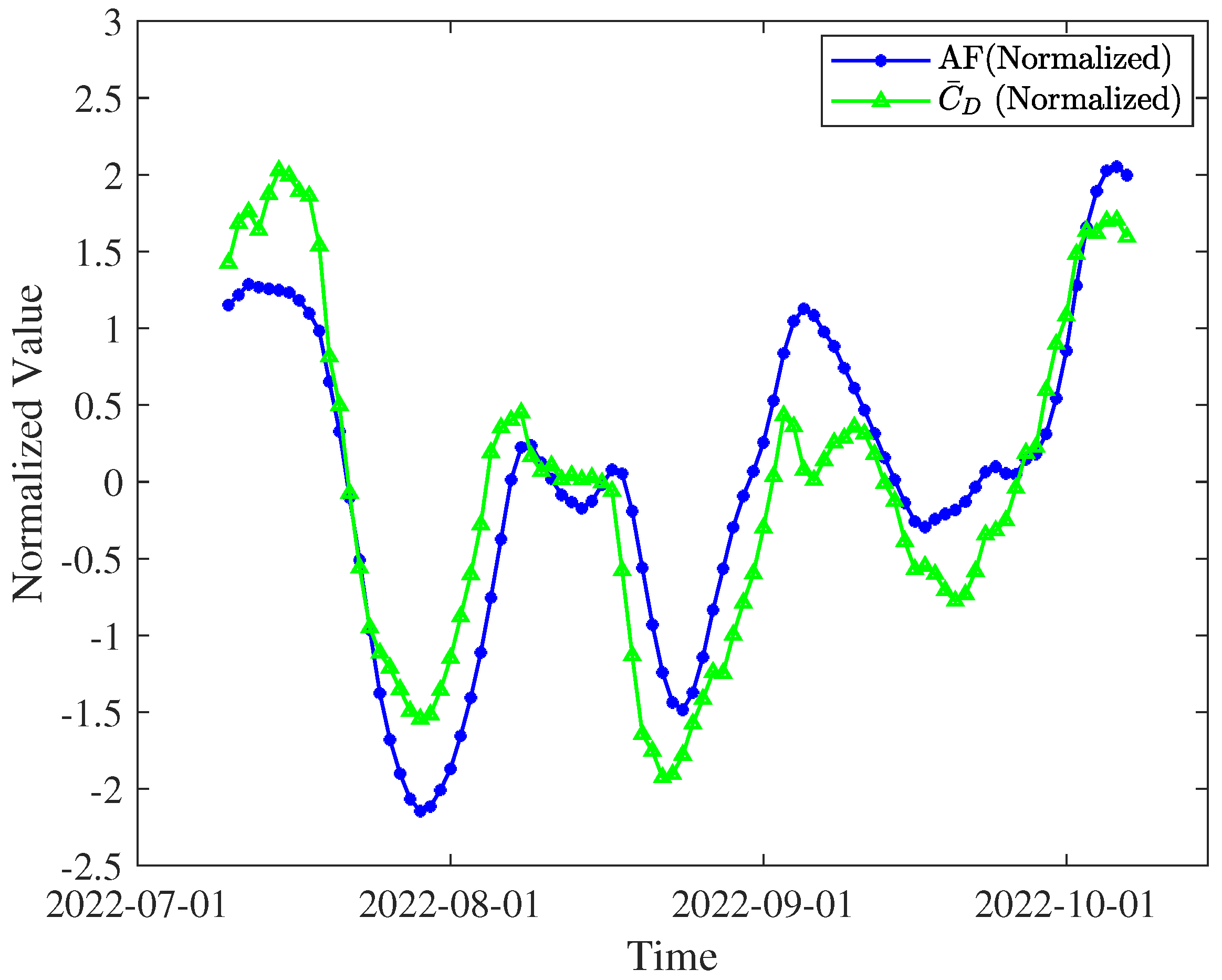
3.3. Correlation of Space Weather and Pseudo-Drag Coefficient

In this paper, changes in space weather are incorporated into the pseudo-drag coefficient ${\overline{C}}_D$ through precise ephemeris rather than being directly calculated from space weather parameters. Geomagnetic and solar activities are key factors affecting atmospheric drag. Therefore, in this section, the relationship between the space weather parameters and the coefficient ${\overline{C}}_D$ is studied in detail. The specific space weather parameters studied are the geomagnetic index $A_P$ and the solar radio flux index $F_{10.7}$. Figure 7 illustrates the changes in $A_P$ and $F_{10.7}$ during the time interval corresponding to Figure 5.

For easier qualitative comparison, the final results are normalized using the formula provided in Equation (17). The Pearson coefficient $r_{XY}$ is used as a quantitative index to evaluate the correlation, and the calculation formula is provided in Equation (18). Figure 5 and Figure 7 are normalized, as shown in Figure 8.

$$x^{\prime }={\displaystyle \frac{x-\mu }{\sigma }},$$

(17)

where $\mu$ and $\sigma$ are the mean and standard deviation of the original data, respectively.

$$r_{XY}={\displaystyle \frac{{\displaystyle \sum _{i=1}^n}(X_i-\overline{X})(Y_i-\overline{Y})}{\sqrt{{\displaystyle \sum _{i=1}^n}{(X_i-\overline{X})}^2{\displaystyle \sum _{i=1}^n}{(Y_i-\overline{Y})}^2}}}.$$

(18)

where $X_i$ and $Y_i$ are the i-th values of variables X and Y, $\overline{X}$ and $\overline{Y}$ are their mean values, respectively, and n is the total number of data.

Figure 8 shows that the overall trend of the ${\overline{C}}_D$ and $F_{10.7}$ is similar, with low-frequency characteristics mainly present, and the $r_{XY}$ is 0.622. The ${\overline{C}}_D$ is affected by the $A_P$ and shows the local correlation in high-frequency characteristics, where $r_{XY}$ is 0.178.

The VMD method enables adaptive frequency decomposition of signals and has advantages in frequency domain feature extraction. Therefore, the VMD method is applied to the $F_{10.7}$ and $A_P$, fusing them into a new space weather feature data set for qualitative analysis, referred to as $AF$. First, the $F_{10.7}$ and $A_P$ are normalized to ensure consistent time-domain amplitude scales, respectively. Next, the normalized results are combined, followed by VMD decomposition to filter out high-frequency components, resulting in the space weather characteristic parameter $AF$. According to the above algorithm, the results of normalizing $AF$ and ${\overline{C}}_D$ are shown in Figure 9.

It is clear from Figure 9 that the $AF$ obtained by VMD has a strong correlation with the ${\overline{C}}_D$, and $r_{XY}$ is 0.879. This demonstrates that the relationship between the $AF$ and the ${\overline{C}}_D$ can be characterized, addressing the second difficulty.

4. OP Based on ML

For a specific satellite, modeling the ${\overline{C}}_D$ using space weather parameters is essentially a regression problem, which is why this study adopts a machine-learning approach. Considering the non-stationarity of space weather change, a VMD-SVM framework for OP is proposed.

4.1. Training Model Using ML

In this paper, the support vector machine (SVM) method is used. The SVM is a supervised machine learning algorithm that can be applied to both classification and regression problems. Its advantage lies in its ability to model both linear and nonlinear problems by selecting appropriate kernel functions. The SVM is an advanced technique proven to be robust against outliers in the dataset, independent of data distribution, possessing general approximation capabilities, and well-suited for processing small sample data. The effectiveness of the SVM method within the orbit prediction framework is demonstrated in this paper. A brief introduction to the SVM method is provided below, with specific details available in the references [36,37].

We assume that the input sample data are $x\in {\mathbf{R}}^m$ and the regression target is $y\in {\mathbf{R}}^m$, with the sample set denoted as $S=\left\{\left(x_i,y_i\right);i=1,2,\cdots ,N\right\}$. The SVM regression method aims to establish a model $f\left(x\right)$ that closely approximates the real regression target y under the insensitive loss of $\epsilon$. In the linear case, the required function is in the following form.

$$f\left(x\right)={\omega }^{T}x+b,$$

(19)

where $\omega$ is a variable and b is a bias. The training problem is formulated as a convex optimization problem.

$$\begin{array}{c}\left\{\begin{array}{c}minJ\left(\omega \right)={\displaystyle \frac{1}{2}}{∥\omega ∥}^2+C{\displaystyle \sum _{i=1}^N}({\xi }_i+{\xi }_i^{\ast })\\ s.t.\left\{\begin{array}{c}{y}_i-{\omega }^{T}x-b\le \epsilon +{\xi }_i\\ {\omega }^{T}x+b-y_i\le \epsilon +{\xi }_i^{\ast }\\ {\xi }_i,{\xi }_i^{\ast }\ge 0\end{array}\right.\end{array}\right.\hfill \end{array},$$

(20)

where $J\left(\omega \right)$ is the cost function, $C>0$ is the penalty factor, $\epsilon$ is the insensitive loss, and ${\xi }_i$ and ${\xi }_i^{\ast }$ are slack variables.

The above solving process is more difficult and needs to be further converted into a dual problem. The Lagrangian multipliers ${\alpha }_i\ge 0$, ${\alpha }_i^{\ast }\ge 0$, ${\eta }_i\ge 0$, and ${\eta }_i^{\ast }\ge 0$ are introduced [37], then the Lagrangian function is

$$\begin{array}{c}L={\displaystyle \frac{1}{2}}{∥\omega ∥}^2+C{\displaystyle \sum _{i=1}^N}({\xi }_i+{\xi }_i^{\ast })-{\displaystyle \sum _{i=1}^N}({\eta }_i{\xi }_i+{\eta }_i^{\ast }{\xi }_i^{\ast })\hfill \\ -{\displaystyle \sum _{i=1}^N}{\alpha }_i(\epsilon +{\xi }_i-y_i+f\left(x_i\right))\hfill \\ -{\displaystyle \sum _{i=1}^N}{\alpha }_i^{\ast }(\epsilon +{\xi }_i^{\ast }+y_i-f\left(x_i\right))\hfill \end{array},$$

(21)

where L computes the partial derivatives with respect to $\omega$, b, ${\xi }_i$, and ${\xi }_i^{\ast }$, and we set them to zero.

$$\left\{\begin{array}{c}{\displaystyle \frac{\partial L}{\partial b}}={\displaystyle \sum _{i=1}^N}({\alpha }_i^{\ast }-{\alpha }_i)=0\hfill \\ {\displaystyle \frac{\partial L}{\partial \omega }}=\omega -{\displaystyle \sum _{i=1}^N}({\alpha }_i-{\alpha }_i^{\ast })x_i=0\hfill \\ {\displaystyle \frac{\partial L}{\partial {\xi }_i^{\ast }}}=C-{\alpha }_i^{\ast }-{\eta }_i^{\ast }=0\hfill \\ {\displaystyle \frac{\partial L}{\partial {\xi }_i}}=C-{\alpha }_i-{\eta }_i=0\hfill \end{array},\right.$$

(22)

Substituting these into the Lagrange function (21), the dual problem of the SVM regression model can be obtained:

$$\left\{\begin{array}{c}\begin{array}{c}maxL=-{\displaystyle \frac{1}{2}}{\displaystyle \sum _{i,j=1}^N}({\alpha }_i-{\alpha }_i^{\ast })({\alpha }_j-{\alpha }_j^{\ast })x_i^T{x}_j\\ -\epsilon {\displaystyle \sum _{i=1}^N}({\alpha }_i+{\alpha }_i^{\ast })+{\displaystyle \sum _{i=1}^N}{y}_i({\alpha }_i-{\alpha }_i^{\ast })\end{array}\\ s.t.{\displaystyle \sum _{i=1}^N}({\alpha }_i-{\alpha }_i^{\ast })=0\&{\alpha }_i,{\alpha }_i^{\ast }\in [0,C]\end{array},\right.$$

(23)

The above process satisfies the KKT condition:

$$\begin{array}{c}\hfill \left\{\begin{array}{c}{\alpha }_i(\epsilon +{\xi }_i-y_i+f\left(x_i\right))=0\\ {\alpha }_i^{\ast }(\epsilon +{\xi }_i^{\ast }+y_i-f\left(x_i\right))=0\\ (C-{\alpha }_i){\xi }_i=0\\ (C-{\alpha }_i^{\ast }){\xi }_i^{\ast }=0\end{array},\right.\end{array}$$

(24)

From Equation (22), $\omega ={\displaystyle \sum _{i=1}^N}({\alpha }_i-{\alpha }_i^{\ast })x_i$; therefore, the final model function is as follows:

$$f\left(x\right)={\displaystyle \sum _{i=1}^N}({\alpha }_i-{\alpha }_i^{\ast })x_i^{T}x+b,$$

(25)

By comparing Equations (19) and (25), it can be seen that $\omega$ can be fully described as a linear combination of the training data x. This feature of SVM makes it possible to handle nonlinear regression using a kernel. By replacing the inner product $k(·, ·)$ in the above equation with kernel $x_i^{T}x$, the optimization problem is reformulated as follows:

$$f\left(x\right)={\displaystyle \sum _{i=1}^N}({\alpha }_i-{\alpha }_i^{\ast })k(x_i,x)+b.$$

(26)

4.2. Model Design and Application

In the supervised learning modeling presented in this paper, a feature selection framework that integrates domain knowledge with statistical validation is employed. The objective is to select feature variables that possess both clear physical interpretability and statistically significant correlations with the target variable, thereby achieving an organic integration of data-driven analysis and physical principles. Based on this framework, the paper delves into the correlations among $F_{10.7}$, $A_P$, and the pseudo-drag coefficient and utilizes the VMD method to extract the space weather feature variable $AF$, thus fully leveraging the strengths of both data-driven approaches and physical laws.

The intelligent OP method proposed is one that integrates orbit dynamics while maintaining a connection to the physical model rather than fully relying on a data-driven approach. The objective of employing the SVM is to model and predict ${\overline{C}}_D$. The space weather feature variable $AF$, constructed using the VMD method, shows a strong correlation with ${\overline{C}}_D$ and can, therefore, serve as an indispensable feature for the SVM model. Additionally, the equivalent drag coefficient ${\widehat{C}}_D$, which reflects the prediction accuracy of the traditional method, can also serve as a physics-referenced baseline and a feature variable for the SVM model. The ${\overline{C}}_D$ is utilized as the target variable for the SVM model. Once the feature variable X and target variable Y have been defined, a training set $D_{train}=\{(x_1,y_1),\dots ,(x_n,y_n)\}=\{([A{F}_1,{\widehat{C}}_{D1}],{\overline{C}}_{D1}),\dots ,([A{F}_n,{\widehat{C}}_{Dn}],{\overline{C}}_{Dn})\}$ can then be generated. The purpose of the SVM model is to learn the mapping relationship between $Y=f\left(X\right)$. Thus, the third difficulty mentioned in this paper is addressed.

To provide a clear understanding of the implementation process, the VMD-SVM pseudocode is presented in

Table 1. VMD-SVM prediction algorithm.

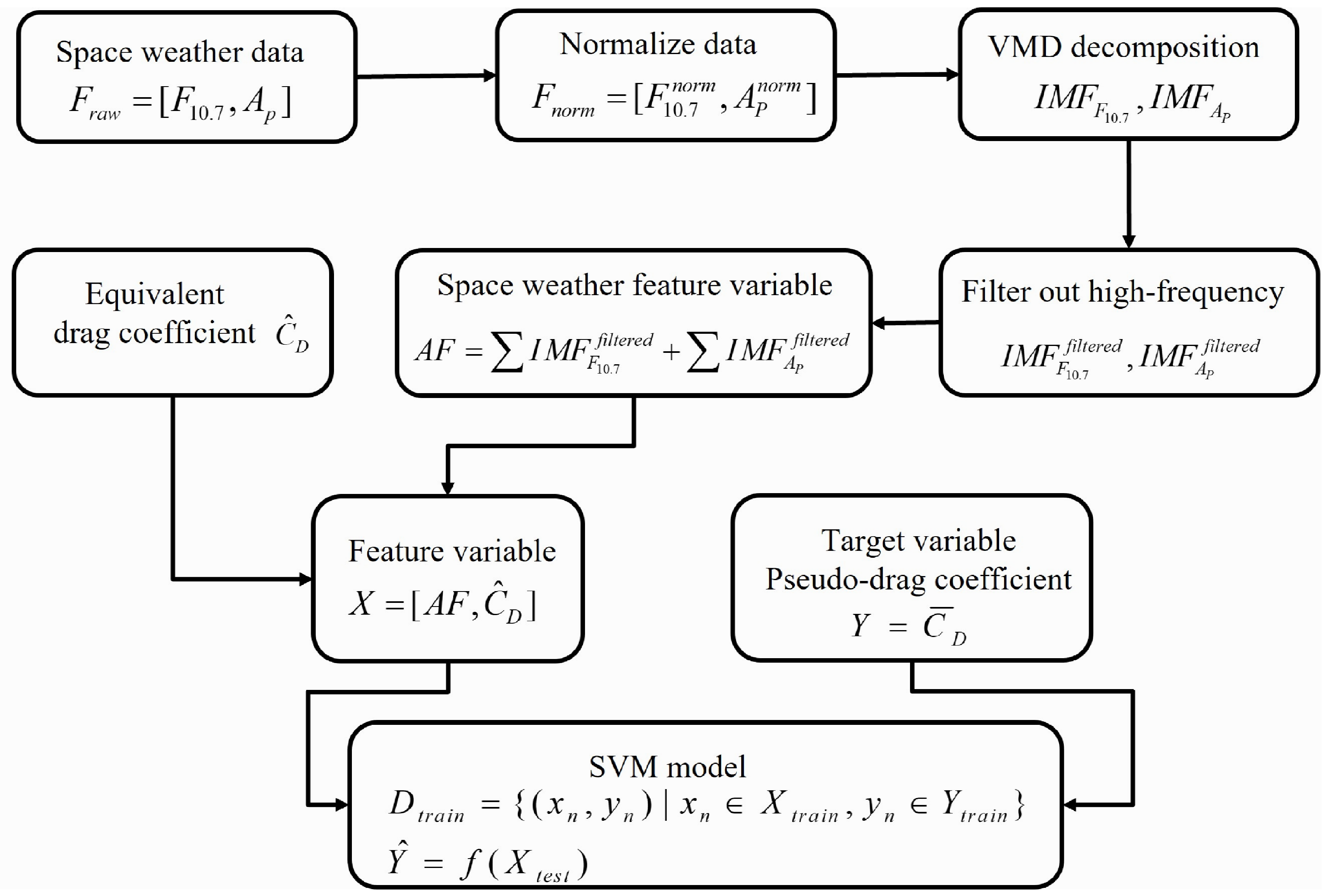
Step	Description
1	Input the original space weather time series data $F_{10.7}$ and $A_P$. Represent the raw data as $F_{raw}=[F_{10.7},A_P]$.
2	Perform data normalization (Z-score) to eliminate dimensional effects. Represent the normalized data as $F_{norm}=[F_{10.7}^{norm},A_P^{norm}]$.
3	Decompose the normalized $F_{10.7}^{norm}$ signal using variational mode decomposition (VMD) into K intrinsic mode functions (IMFs). Represent the IMF components as $IM{F}_{F_{10.7}}=\{IM{F}_{F_{10.7},1},IM{F}_{F_{10.7},2},\dots ,IM{F}_{F_{10.7},K}\}$.
4	Decompose the normalized $A_P^{norm}$ signal using variational mode decomposition (VMD) into K intrinsic mode functions (IMFs). Represent the IMF components as $IM{F}_{A_P}=\{IM{F}_{A_P,1},IM{F}_{A_P,2},\dots ,IM{F}_{A_P,K}\}$.
5	Filter out high-frequency noise components from $IM{F}_{F_{10.7}}$ and $IM{F}_{A_P}$. Represent the filtered IMFs as $IM{F}_{F_{10.7}}^{filtered}$ and $IM{F}_{A_P}^{filtered}$.
6	Construct the space weather feature variable $AF$ by summing all the remaining filtered IMFs from both $F_{10.7}$ and $A_P$. Represent the accumulated feature as $AF=\sum IM{F}_{F_{10.7}}^{filtered}+\sum IM{F}_{A_P}^{filtered}$.
7	Combine $AF$ with the equivalent drag coefficient ${\widehat{C}}_D$ to form the input feature X, represented as $X=[AF,{\widehat{C}}_D]$.
8	Divide the dataset into a training set $D_{train}=\{X_{train},Y_{train}\}$ and a testing set $D_{test}=\{X_{test},Y_{test}\}$ in chronological order.
9	Define the target variable as $Y={\overline{C}}_D$, with the training set represented as $D_{train}=\left\{(x_n,y_n)\right|x_n\in X_{train},y_n\in Y_{train}\}$.
10	Select the radial basis function (RBF) as the kernel for the support vector machine (SVM) and initialize the hyperparameters.
11	Train the SVM model on $D_{train}$ by iteratively optimizing the model parameters to minimize the prediction error on the training set.
12	Input the testing set $X_{test}$ and use the trained SVM model to predict the output $\widehat{Y}=f\left(X_{test}\right)$, achieving pseudo-drag coefficient prediction.

, while the corresponding flowchart is illustrated in Figure 10.

4.3. Performance Metric

In this paper, a metric for evaluating the accuracy of OP is proposed. The OP error of the proposed method is defined as ${\mathit{e}}_{ML}$, and the OP error calculated by the traditional method is defined as ${\mathit{e}}_{Trad}$. The calculation method is as follows:

$${\mathit{e}}_i\left(t_k\right)={\mathit{x}}_i(t_k;t_0)-{\mathit{x}}_{\mathrm{true}}\left(t_k\right),$$

(27)

where $i\in \{\mathrm{ML}, \mathrm{Trad}\}$ represents this paper and the traditional method, respectively. ${\mathit{x}}_{\mathrm{true}}\left(t_k\right)$ is the true position and velocity vectors at time $t_k$, and ${\mathit{x}}_i(t_k;t_0)$ is the predicted position and velocity vectors at time $t_k$.

The root mean square error $RMS$ is used to evaluate the prediction accuracy and the performance metric $PM$ is used to quantify the effectiveness of the proposed method in improving OP accuracy, which is defined as follows:

$$PM=(1-{\displaystyle \frac{RM{S}_{pos,ML}}{RM{S}_{pos,Trad}}})\times 100\%,$$

(28)

where $RMS$ is calculated according to Equation (29), where N denotes the number of error sampling points.

$$RM{S}_{pos,i}=\sqrt{{\displaystyle \frac{1}{N}}{\displaystyle \sum _{k=1}^N}{∥e_i^{pos}\left(t_k\right)∥}_2^2},i\in \{\mathrm{ML},\mathrm{Trad}\}.$$

(29)

where ${\mathit{e}}_i^{\mathrm{pos}}\left(t_k\right)$ is the position error vector in ${\mathit{e}}_i\left(t_k\right)$.

The performance metric $PM$ primarily assesses the improvement in prediction accuracy of the proposed method compared to the traditional method. When the proposed method predicts accurately, $PM$ is positive, with the theoretical optimal value being close to 100%. If the prediction performance of the model is not ideal, the $PM$ value will be close to 0 or even negative.

5. Experimental Results

5.1. Experimental Background and Data Preparation

To verify the effectiveness of the proposed method, three satellites with orbit heights of 400 km, 500 km, and 600 km are selected for the experiments, which were named SAT1, SAT2, and SAT3. The prediction duration is 10 days, and the prediction error results are based on the traditional OD/OP method and the VMD-SVM method for LEO satellites with different orbital heights. Before training, the space weather parameters are decomposed via VMD, and the pseudo-drag coefficient and the equivalent-drag coefficient are solved to prepare the dataset for SVM. The data processing and model design methods involved were elaborated in the previous section and are not repeated here.

5.2. ML-Based OP and Quantitative Analysis

The experiment utilizes uncontrolled satellite observation data spanning 100 consecutive days, and the first 70 days of data are used to establish a pseudo-drag coefficient set as a training set label for the machine learning model. It should be noted that when establishing the pseudo-drag coefficient set, since the prediction time is set to 10 days, each calculation of a pseudo-drag coefficient requires 10 days of precise ephemeris data. Therefore, the 70-day data can be used to establish a dataset containing 60 pseudo-drag coefficients for ML training. However, in the prediction stage, the start epoch begins on the 70th day, so the 70th pseudo-drag coefficient is needed for prediction.

In practical applications, the generalization ability of the model is important. To verify the generalization and effectiveness of the proposed method in orbit prediction, 20 independent experiments are conducted for each satellite using the remaining 30 days’ precise ephemeris data. Three cases are designed as follows:

Case 1: The satellite SAT1, with an orbit height of about 400 km, is predicted for 10 days, and 20 sets of independent experiments are carried out. The experimental results are shown in Figure 11 and Figure 12.

Case 2: The satellite SAT2, with an orbit height of about 500 km, is predicted for 10 days, and 20 sets of independent experiments are carried out. The experimental results are shown in Figure 13 and Figure 14.

Case 3: The satellite SAT3, with an orbit height of about 600 km, is predicted for 10 days, and 20 sets of independent experiments are carried out. The experimental results are shown in Figure 15 and Figure 16.

For three satellite cases, the orbit prediction error results are normalized by Equation (6). The prediction and reference results of the training set and test set of the ML model are shown in Figure 11a, Figure 13a, and Figure 15a. Furthermore, the relative error results of the test set predicted pseudo-drag coefficient and the equivalent-drag coefficient relative to the reference value of the pseudo-drag coefficient are shown in Figure 11b, Figure 13b and Figure 15b, respectively. The relative error of the VMD-SVM method is less than that of the equivalent-drag coefficient, indicating that the OP results of the VMD-SVM method may be better than those of the traditional method. The specific quantitative results are assessed by the $PM$ value. The orbit prediction errors of the first set of experiments in the RAC coordinate system are shown in Figure 12a–c, Figure 14a–c, and Figure 16a–c, and the $PM$ values of the 20 sets of experiments are shown in Figure 12d, Figure 14d, and Figure 16d, respectively.

Compared to current traditional methods, the results show that the method proposed in this paper can effectively improve OP accuracy. For the three satellites, the $PM$ values indicate that the rates of effective improvement in OP are 85%, 85%, and 80% in 20 experiments, which are consistent with the relative error comparison results shown in Figure 11b, Figure 13b and Figure 15b, respectively. The optimal improvement effects for the three cases can reach up to 67.20%, 89.56%, and 92.45%, with the first set of experiments showing improvements of 59.72%, 56.86%, and 75.48%, respectively. In addition, the OP error reveals that the along-track error is the main source of error for LEO satellites, with the error direction varying. The VMD-SVM method, developed in this paper based on the concept of the pseudo-drag coefficient, exhibited satisfactory overall performance in practical OP applications.

In this paper, the specific computer test environment was configured as follows: Intel(R) Core(TM) i9-14900HX @ 2.20 GHz, 64 GB RAM, 4 TB SSD, RTX 4070 GPU, and Windows 11(64-bit). To evaluate the computational efficiency of the VMD-SVM method, a corresponding computational experiment was conducted. Under the premise of the given dataset, which includes the raw space weather $F_{10.7}$ and $A_P$ (requiring VMD decomposition), along with the required equivalent drag coefficient ${\widehat{C}}_D$ (as one of the feature variables) and pseudo-drag coefficient ${\overline{C}}_D$ (as the target variable) dataset, a single 10-day orbit prediction was performed in the validation experiment, with the VMD-SVM framework achieving a computation time of approximately 4 seconds.

6. Conclusions

In this paper, the concept of the pseudo-drag coefficient was defined, and the VMD-SVM orbit prediction strategy was proposed to improve the performance of the traditional OD/OP method. Specifically, the space weather and atmospheric drag model were related through the pseudo-drag coefficient, and the strong correlation between the space weather and pseudo-drag coefficient was discovered using the VMD technique. Thus, the OP problem was transformed into a pseudo-drag coefficient prediction problem. Then, the pseudo-drag coefficient was predicted using the SVM method, significantly improving the precision of OP when combined with the traditional OP dynamics model. Furthermore, medium and long-term OP verification experiments were conducted using observation data from satellites with orbital altitudes from 400 km to 600 km. The practicality and effectiveness of the proposed method were proved by the experimental results.

Additionally, the overall VMD-SVM orbit prediction framework can be developed as an auxiliary system that integrates with traditional methods, enabling convenient synchronous use and facilitating future upgrades. In future work, we will consider incorporating more characteristic variables without preprocessing the space weather parameters, simplifying the workflow while maintaining the overall performance of the method and enhancing the interpretability of the machine learning model.

References

- Lal, B.; Balakrishnan, A.; Caldwell, B.M.; Buenconsejo, R.S.; Carioscia, S.A. Global Trends in Space Situational Awareness (SSA) and Space Traffic Management (STM); Institute for Defense Analyses: Frederick, MD, USA, 2022. [Google Scholar]
- Yue, P.; An, J.; Zhang, J.; Ye, J.; Pan, G.; Wang, S.; Xiao, P.; Hanzo, L. Low earth orbit satellite security and reliability: Issues, solutions, and the road ahead. IEEE Commun. Surv. Tutor. 2023, 25, 1604–1652. [Google Scholar] [CrossRef]
- Zhang, Z.; Shi, Y.; Zheng, Z. Improving Angle-Only Orbit Determination Accuracy for Earth–Moon Libration Orbits Using a Neural-Network-Based Approach. Remote Sens. 2024, 16, 3287. [Google Scholar] [CrossRef]
- Vallado, D.A. Fundamentals of Astrodynamics and Applications; Springer Science & Business Media: Berlin/Heidelberg, Germany, 2001. [Google Scholar]
- Chen, L.; Bai, X.Z.; Liang, Y.G.; Li, K.B.; Chen, L.; Bai, X.Z.; Li, K.B. Orbital Prediction Error Propagation of Space Objects. In Orbital Data Applications for Space Objects: Conjunction Assessment and Situation Analysis; Springer: Berlin/Heidelberg, Germany, 2017; pp. 23–75. [Google Scholar]
- McLaughlin, C.A.; Hiatt, A.; Lechtenberg, T. Precision orbit derived total density. J. Spacecr. Rocket. 2011, 48, 166–174. [Google Scholar] [CrossRef]
- Emmert, J.T.; Warren, H.P.; Segerman, A.M.; Byers, J.M.; Picone, J.M. Propagation of atmospheric density errors to satellite orbits. Adv. Space Res. 2017, 59, 147–165. [Google Scholar] [CrossRef]
- Peng, H.; Bai, X. Artificial neural network-based machine learning approach to improve orbit prediction accuracy. J. Spacecr. Rocket. 2018, 55, 1248–1260. [Google Scholar] [CrossRef]
- Peng, H.; Bai, X. Exploring capability of support vector machine for improving satellite orbit prediction accuracy. J. Aerosp. Inf. Syst. 2018, 15, 366–381. [Google Scholar] [CrossRef]
- Peng, H.; Bai, X. Improving orbit prediction accuracy through supervised machine learning. Adv. Space Res. 2018, 61, 2628–2646. [Google Scholar] [CrossRef]
- Peng, H.; Bai, X. Gaussian processes for improving orbit prediction accuracy. Acta Astronaut. 2019, 161, 44–56. [Google Scholar] [CrossRef]
- Li, B.; Zhang, Y.; Huang, J.; Sang, J. Improved orbit predictions using two-line elements through errors pattern mining and transferring. Acta Astronaut. 2021, 188, 405–415. [Google Scholar] [CrossRef]
- Zhai, M.; Huyan, Z.; Hu, Y.; Jiang, Y.; Li, H. Improvement of orbit prediction accuracy using extreme gradient boosting and principal component analysis. Open Astron. 2022, 31, 229–243. [Google Scholar] [CrossRef]
- Huang, W.; Tang, R.; Qu, G.; Zhang, F. An XGBoost-Based Method for Improved Orbit Prediction With an Orbit-Separate Modeling Strategy. IEEE Trans. Aerosp. Electron. Syst. 2024, 60, 4887–4895. [Google Scholar] [CrossRef]
- Peng, H.; Bai, X. Fusion of a machine learning approach and classical orbit predictions. Acta Astronaut. 2021, 184, 222–240. [Google Scholar] [CrossRef]
- Peng, H.; Bai, X. A medium-scale study of using machine learning fusion to improve TLE prediction precision without external information. Acta Astronaut. 2023, 204, 477–491. [Google Scholar] [CrossRef]
- Haidar-Ahmad, J.; Khairallah, N.; Kassas, Z.M. A hybrid analytical-machine learning approach for LEO satellite orbit prediction. In Proceedings of the 2022 25th International Conference on Information Fusion, Linköping, Sweden, 5 July 2022. [Google Scholar]
- Marcos, F.A. Accuracy of atmospheric drag models at low satellite altitudes. Adv. Space Res. 1990, 10, 417–422. [Google Scholar] [CrossRef]
- Doornbos, E.; Klinkrad, H. Modelling of space weather effects on satellite drag. Adv. Space Res. 2006, 37, 1229–1239. [Google Scholar] [CrossRef]
- Storz, M.F.; Bowman, B.R.; Branson, M.J.I.; Casali, S.J.; Tobiska, W.K. High accuracy satellite drag model (HASDM). Adv. Space Res. 2005, 36, 2497–2505. [Google Scholar] [CrossRef]
- Emmert, J.T. Thermospheric mass density: A review. Adv. Space Res. 2015, 56, 773–824. [Google Scholar] [CrossRef]
- Picone, J.M.; Emmert, J.T.; Lean, J.L. Thermospheric densities derived from spacecraft orbits: Accurate processing of two-line element sets. J. Geophys. Res.-Space Phys. 2005, 110, A03301. [Google Scholar] [CrossRef]
- Doornbos, E.; Klinkrad, H.; Visser, P.N.A.M. Atmospheric density calibration using satellite drag observations. Adv. Space Res. 2005, 36, 515–521. [Google Scholar] [CrossRef]
- Bruinsma, S.; Tamagnan, D.; Biancale, R. Atmospheric densities derived from CHAMP/STAR accelerometer observations. Planet Space Sci. 2004, 52, 297–312. [Google Scholar] [CrossRef]
- Sutton, E.K.; Nerem, R.S.; Forbes, J.M. Density and winds in the thermosphere deduced from accelerometer data. J. Spacecr. Rocket. 2007, 44, 1210–1219. [Google Scholar] [CrossRef]
- Calabia, A.; Jin, S. New modes and mechanisms of thermospheric mass density variations from GRACE accelerometers. J. Geophys. Res.-Space Phys. 2016, 121, 191–212. [Google Scholar] [CrossRef]
- Calabia, A.; Jin, S. Thermospheric density estimation and responses to the March 2013 geomagnetic storm from GRACE GPS-determined precise orbits. J. Atmos. Sol.-Terr. Phys. 2017, 154, 167–179. [Google Scholar] [CrossRef]
- Calabia, A.; Jin, S. Upper-Atmosphere Mass Density Variations From CASSIOPE Precise Orbits. Space Weather 2021, 19, e2020SW002645. [Google Scholar] [CrossRef]
- Pérez, D.; Bevilacqua, R. Neural Network based calibration of atmospheric density models. Acta Astronaut. 2015, 110, 58–76. [Google Scholar] [CrossRef]
- Sakai, T.; Takahashi, Y. Atmospheric Density Estimation in Very Low Earth Orbit Based on Nanosatellite Measurement Data Using Machine Learning. Aerosp. Sci. Technol. 2024, 153, 109418. [Google Scholar] [CrossRef]
- Weng, L.; Lei, J.; Zhong, J.; Dou, X.; Fang, H. A machine-learning approach to derive long-term trends of thermospheric density. Geophys. Res. Lett. 2020, 47, e2020GL087140. [Google Scholar] [CrossRef]
- Wang, R.; Liu, J.; Zhang, Q.M. Propagation errors analysis of TLE data. Adv. Space Res. 2009, 43, 1065–1069. [Google Scholar] [CrossRef]
- Cimmino, N.; Opromolla, R.; Fasano, G. Machine learning-based approach for ballistic coefficient estimation of resident space objects in LEO. Adv. Space Res. 2023, 71, 5007–5025. [Google Scholar] [CrossRef]
- Paul, S.N.; Sheridan, P.L.; Licata, R.J.; Mehta, P.M. Stochastic modeling of physical drag coefficient–Its impact on orbit prediction and space traffic management. Adv. Space Res. 2023, 72, 922–939. [Google Scholar] [CrossRef]
- Dragomiretskiy, K.; Zosso, D. Variational mode decomposition. IEEE Trans. Signal Process. 2013, 62, 531–544. [Google Scholar] [CrossRef]
- Hammer, B.; Gersmann, K. A note on the universal approximation capability of support vector machines. Neural Process. Lett. 2003, 17, 43–53. [Google Scholar] [CrossRef]
- Smola, A.J.; Schölkopf, B. A tutorial on support vector regression. Stat. Comput. 2004, 14, 199–222. [Google Scholar] [CrossRef]