Abstract
The permanently shadowed regions of the lunar South Pole have become a key target for international lunar exploration due to their unique scientific value and engineering challenges. In order to effectively screen suitable landing zones near the lunar South Pole, this research proposes a comprehensive evaluation method based on a self-organizing map (SOM). Using multi-source remote sensing data, the method classifies and analyzes candidate landing zones by combining scientific purposes (such as hydrogen abundance, iron oxide abundance, gravity anomalies, water ice distance analysis, and geological features) and engineering constraints (such as Sun visibility, Earth visibility, slope, and roughness). Through automatic clustering, the SOM model finds the important regions. Subsequently, it integrates with a supervised learning model, a random forest, to determine the feature importance weights in more detail. The results from the research indicate the following: the areas suitable for landing account for 9.05%, 5.95%, and 5.08% in the engineering, scientific, and synthesized perspectives, respectively. In the weighting analysis of the comprehensive data, the weights of Earth visibility, hydrogen abundance, kilometer-scale roughness, and slope data all account for more than 10%, and these are thought to be the four most important factors in the automated site selection process. Furthermore, the kilometer-scale roughness data are more important in the comprehensive weighting, which is in line with the finding that the kilometer-scale roughness data represent both surface roughness from an engineering perspective and bedrock geology from a scientific one. In this study, a local examination of typical impact craters is performed, and it is confirmed that all 10 possible landing sites suggested by earlier authors are within the appropriate landing range. The findings demonstrate that the SOM-model-based analysis approach can successfully assess lunar South Pole landing areas while taking multiple constraints into account, uncovering spatial distribution features of the region, and offering a rationale for choosing desired landing locations.
1. Introduction
Because of its exceptional potential to answer important scientific issues, the lunar South Pole has become a top target for further exploration [1,2,3]. Over geological timeframes, volatiles like water ice can be trapped in permanently shadowed regions (PSRs), which are created by the Moon’s slight axial tilt of 1.5°. In addition to providing in situ resources for sustainable human exploration and the establishment of lunar bases, these volatiles are crucial for understanding the formation and evolution of the Moon [4,5].
Compared to the North Pole, the lunar South Pole has a greater number of large PSRs and adjacent elevated terrains that receive near-constant sunlight [6,7,8,9]. It also overlaps with the South Pole-Aitken (SPA) Basin, one of the oldest and deepest impact basins in the solar system, making it an important region for sampling early lunar crust and understanding the inner solar system’s impact history [10,11,12,13].
In response to this scientific and strategic value, multiple nations have launched or are planning polar exploration missions, including NASA’s Artemis program and VIPER rover [14,15], the ESA’s HERACLES mission [16], the ISRO’s Chandrayaan missions [17], ROSCOSMOS’s Luna-25 [18], and China’s Chang’E program [19]. These missions share a common challenge: selecting safe and scientifically valuable landing sites within complex polar terrains.
Landing site selection at the lunar South Pole must balance multiple and often conflicting objectives: scientific return, engineering feasibility, resource accessibility, and long-term sustainability [20]. Traditional selection methods, such as multi-criteria decision analysis and expert-guided models [3,17,21], have played a critical role in enabling early identification of candidate regions, integrating expert knowledge with available remote sensing data, and providing structured decision frameworks to inform mission planning and risk assessment. These approaches were especially useful when data were limited or expert judgment was required. However, they frequently rely on subjective weighting, are susceptible to prior assumptions, and struggle with high-dimensional, multi-source remote sensing datasets. Furthermore, manually integrating multiple data layers and engaging in expert consultation processes can be time-consuming and labor-intensive [22]. These constraints limit the scalability and efficiency of standard approaches when applied to vast and complex polar terrains.
Recent advances in machine learning have allowed for data-driven techniques to evaluate lunar landing sites. Supervised learning methods, such as weighted ranking models [23], extreme gradient boosting models [24], and CNN-based scoring systems [25], have demonstrated promise by leveraging labeled data to attain high prediction accuracy and interpretable decision-making in well-characterized regions. However, their effectiveness is limited by the scarcity of labeled landing site data, particularly in unexplored regions. Clustering-based approaches [26,27] provide an alternative, although they frequently fail to adequately integrate various scientific and engineering restrictions.
To address these limitations, this study presents an unsupervised learning framework based on the self-organizing map (SOM) algorithm [28], which is ideal for extracting latent patterns from high-dimensional geospatial data. SOM has been widely used in remote sensing for unsupervised classification, land cover analysis, and pattern recognition, especially in cases requiring high-dimensional and multi-source data, when labeled samples are limited or unavailable [29]. In contrast to conventional techniques, SOM eliminates human bias and subjective assumptions by automatically clustering regions based on the underlying structure of the input data without the need for labeled data. It is useful for recognizing different kinds of data, displaying their distribution, and assessing their landing suitability because of its capacity to capture nonlinear dependencies and project multidimensional input into a two-dimensional network.
A sliding-window preprocessing technique is presented in order to further minimize spatial bias and the possibility of missing appropriate micro-regions. This guarantees that local spatial details are not overlooked and permits ongoing assessment throughout the lunar South Polar region [26]. By minimizing trial and error and enhancing model stability, Bayesian optimization is used to identify important hyperparameters such as grid size and iteration in order to maximize the performance of the SOM model.
Moreover, the feature importance analysis based on a random forest is performed on the clustering results to improve interpretability and evaluate the influence of various characteristics. This hybrid SOM and random forest framework offers a thorough assessment model by combining the interpretability of supervised learning with the scalability and data-driven structure discovery of unsupervised learning.
Above all, the objective of this research is to develop an intelligent, interpretable, and automated evaluation model for selecting landing zones in the lunar South Pole. The proposed framework integrates a variety of scientific factors, such as hydrogen abundance, kernel density analysis of geological maps, distance analysis of exposed water ice, iron oxide abundance, and gravity anomalies, along with engineering factors like solar illumination, communication, slope, and surface roughness. Using this extensive data set, the framework can handle nonlinear relationships, avoid the need for subjective weights, and ensure full spatial coverage. This makes it an effective tool for future polar exploration missions, as it provides a data-driven approach to optimal landing site selection.
2. Study Area and General Framework
2.1. Study Area
The lunar South Pole, as an important area for lunar scientific exploration, holds unique scientific value and exploration potential. Located at the edge of the South Pole-Aitken (SPA) Basin, the terrain is rough, and extreme lighting conditions prevail due to the Moon’s small axial inclination [9,13,30]. Despite this, certain locations within the region, such as the areas near the Shackleton Crater and De Gerlach Crater, as well as the ridge connecting them, have areas that receive nearly continuous sunlight for over 80% of the time, providing ideal locations for future scientific missions [31,32]. Additionally, the solar panel lighting conditions can be significantly improved with minimal height gain (2–10 m), providing a stable power supply and making these regions key targets for future lunar exploration missions [8,33,34].
The lunar South Pole’s average annual surface temperature is as low as 38 K, with the PSRs having temperatures low enough to effectively trap condensed volatiles such as water ice [35,36]. Remote sensing data show that water ice may exist on the surface or subsurface of some PSRs, with a strong correlation between surface ice and surface reflectance anomalies from the Lyman Alpha Mapping Project (LAMP) and LOLA 1064 nm data, supporting the theory of water ice in these regions [37]. Moreover, the Moon Mineralogy Mapper (M3) data reveal diagnostic near-infrared absorption features of water ice [38]. Hydrogen concentration data from the Lunar Energetic Neutron Detector (LEND) and LPNS estimate the water-equivalent hydrogen (WEH) value in the South Pole area to be 0.3–0.5 wt.%, indicating potential deposits of water ice and other volatile substances [39,40].
These characteristics of the lunar South Pole not only offer favorable environmental conditions for future long-term exploration on the Moon but also provide valuable insights into the volatile substance evolution of the solar system [41]. Recent observations, such as the impact plume from the LCROSS mission, revealed the presence of water ice and other volatile compounds, such as light hydrocarbons, sulfur compounds, and carbon dioxide, further confirming the South Pole’s importance as a region for resource collection and energy utilization [42]. Additionally, the coexistence of high-illumination peaks and PSRs at the South Pole offers unique opportunities for solar energy utilization and resource exploration [41,43]. These areas could contain frozen volatiles for consumables, radiation shielding, and propellants necessary for human habitation. Therefore, the lunar South Pole is not only a crucial area for scientific exploration but also a key location for future lunar exploration and utilization.
In an effort to resolve the debate over the presence of water ice and other cold-trapped volatiles at the lunar poles [2,36,38,44,45], different regions and organizations have announced new rounds of lunar South Pole exploration plans, as shown in Figure 1 and Table 1. This overview provides important context for the fundamental geographic distribution of landing site selections, and some of the sites listed are mentioned in the regional analysis presented in Section 4.3.
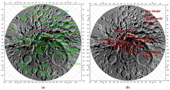
Figure 1.
(a) WAC image map of the lunar South Pole superimposed with lunar place names and (b) landing sites associated with the lunar South Pole, with corresponding mission details provided in Table 1.

Table 1.
Lunar South Pole exploration plans.
2.2. Framework
The general framework of SOM-based South Polar landing zone selection is given in Figure 2. This research uses a feature-level fusion strategy based on SOM to integrate multi-source scientific and engineering data, such as slope, Sun visibility, Earth visibility, and roughness, as well as water ice exposure, South Pole geologic maps, iron oxide abundance, gravity anomalies, and hydrogen abundance. The technique entails first resampling all input data to a consistent spatial resolution, then creating 10-dimensional feature vectors (corresponding to 10 input data sources) for each geographical unit, and finally applying min–max normalization to reduce scale variations.
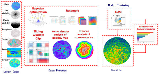
Figure 2.
Schematic of SOM-based South Polar landing zone selection.
To address hyperparameter optimization in the SOM model, a Bayesian optimization technique automatically identifies the best network topology and training epoch and predicted improvement acquisition functions for efficient parameter space exploration. The input layer’s neuron count is directly proportional to the data source dimensions (10 neurons for 10 data sources in the full model, or 5 neurons for 5 data sources in the engineering model), and all preprocessed feature data are supplied into the network at the same time.
The SOM automatically discovers nonlinear correlations between features using its competitive learning mechanism, resulting in synergistic grouping of multi-source data. To improve interpretability, post-training random forest analysis computes significance scores, which quantify each feature’s contribution to clustering outcomes.
The final output neuron weight vectors indicate the best feature combination patterns, allowing for unsupervised clustering-based landing site selection. This strategy takes full advantage of SOM’s topology-preserving properties to successfully retain high-dimensional feature associations in low-dimensional mapping space. By combining Bayesian optimization for automated parameter selection and random forest for feature importance analysis, the method achieves high-performance and interpretable data-driven feature-level fusion, offering dependable technological support for lunar South Polar landing site selection.
3. Materials and Methods
3.1. Data
For decades, research institutions and organizations have collected a large amount of remote sensing data that provide critical information on the presence or absence of cold-captured volatiles on the Moon. These data are categorized into engineering and scientific categories, and they include slope, Sun visibility, Earth visibility, and roughness, as well as water ice exposure, South Pole geologic maps, iron oxide abundance, gravity anomalies, and hydrogen abundance, as shown in Figure 3 and Table 2.
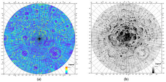
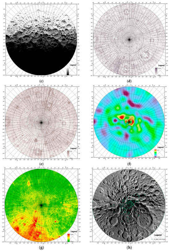
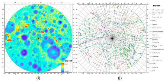
Figure 3.
Summary of lunar South Pole data: (a–j) slope, Sun visibility, Earth visibility, roughness at the hm and km scales, hydrogen abundance, iron oxide content, exposed water ice, gravity anomalies, and a geological map. (a) Slope, (b) Sun visibility, (c) Earth visibility, (d) hectometer-scale roughness, (e) kilometer-scale roughness, (f) hydrogen abundance, (g) FeO, (h) exposed water ice, (i) gravity anomalies, and (j) geological map.
Table 2.
Summary table of lunar South Pole remote sensing data.
Engineering category:
Slope: The LOLA team mapped products describing the slope of the lunar surface at a resolution of 255 ppd (120 m over the equator) based on shape data from SLDEM2015 [46,47], and they are available from the Planetary Data System LOLA Data node (http://imbrium.mit.edu/EXTRAS/SLDEM2015/ (accessed on 18 June 2018)).
Sun visibility (illumination) and Earth visibility: LOLA-based solar and Earth visibility is obtained by time-averaging the results of computational modeling performed hourly for about 18.6 years, with a resolution of 240 m/pixel [9]. Mean visibility is a fraction of time equal to 0 when the Sun/Earth is not visible and 1 when any part of the Sun/Earth is visible. Illumination values represent the proportion of time that the Sun is visible from a given location.
Roughness: Kreslavsky et al. provided maps of the roughness of the lunar terrain on scales of meters and kilometers, derived from distance profiles obtained by the LOLA instrument (the Lunar Orbiting Laser Altimeter) onboard the Lunar Reconnaissance Orbiter LRO spacecraft, revealing features of the terrain that could not be analyzed with LOLA-based raster topographic maps at a resolution of 16 ppd [48].
Scientific category:
FeO: Lemelin et al. obtained an absolute reflectance data cube based on the Kaguya Spectral Profiler dataset depicting the first map of iron oxide (FeO) minerals in the polar regions with a spatial resolution of 1 km/pixel [49].
Hydrogen Abundance Map: Peplowski et al. corrected for variations in rare-earth elements by conducting an analysis similar to that of scholars who quantitatively understood rare-earth and thermal neutron variations [50]. A key aspect of this correction uses a quantitative baseline of rare earth element variations in the composition of lunar samples and applies these corrections to orbital data, yielding a complete global map of bulk hydrogen abundances across the lunar surface.
Gravity: GRAIL free-air gravity or gravitational perturbations were obtained at 16 pixels/degree with a reference radius of 1738 km using the GRGM1200A gravity model with an expansion of L = 660. They show the “free-air” variations as measured by the spacecraft and, therefore, include contributions from the surface relief and from any subsurface interfaces [51].
PSR: This study calculated horizon elevations in the polar regions (up to ∼75° latitude) from LOLA data and modeled the lighting conditions in the two polar regions (extending to ~80° latitude) to obtain the locations of the permanently shaded areas and the polar regions that are most well illuminated [9].
Geological map: Jinzhu Ji et al. [52] provided a 1:2,500,000 scale global geological map of the Moon, mainly using data from the China Lunar Exploration Project (CLEP) and international exploration missions, with distortions reduced by the division of 30 regions with different map projections, and mapped using the ESRI ArcMap platform. The lunar geological map is divided into three periods, Eolunarian, Paleolunarian, and Neolunarian, according to the geological time scale, and defines 90 geological units covering impact craters, basin formation, endogenous orogeny, and so on. The map illustrates lunar impact basins, craters, rock types, and geological structures, providing key data on the Moon’s geological evolution and support for lunar base construction.
Water ice exposure: The process of detecting surface-exposed water ice in the lunar polar regions involves using near-infrared (NIR) reflectance spectral data obtained from the Moon Mineralogy Mapper (M3). After thermal calibration and projection processing, shadowed regions are identified by combining LOLA topographic data. By analyzing the absorption features of water ice in the spectra and comparing them with laboratory water ice spectra, the presence and distribution of water ice are ultimately confirmed [38].
In the selection of lunar South Pole landing sites, the above data can be used for a comprehensive assessment of the suitability of candidate regions. Slope, illumination, Earth visibility, and roughness are engineering factors that directly impact landing safety and mission feasibility; for example, smaller slopes aid in stable landings, areas with continuous illumination provide reliable energy, good communication conditions ensure data transmission, and lower surface roughness reduces mechanical damage risks. However, water ice exposure, South Pole geological maps, iron oxide abundance, gravity anomalies, and hydrogen abundance are scientific factors that determine the research value and resource utilization potential of landing sites. For example, water ice resources can be used for fuel production and life support; geological features reveal the moon’s evolutionary history; ilmenite (FeTiO₃), concentrated in high-FeO terrains (lunar maria), offers a readily reducible source of oxygen and titanium for in situ construction and manufacturing and can be a potential source of helium-3 [53,54]; gravity anomalies reflect subsurface structures; and hydrogen abundance suggests possible volatile distributions. Through the SOM method, these factors can be comprehensively analyzed to identify the optimal landing regions that satisfy both engineering and scientific requirements.
3.2. Method
A self-organizing map (SOM) is an unsupervised learning algorithm. The proposed artificial neural network is capable of mapping high-dimensional data into a low-dimensional representation space. It is a popular tool for high-dimensional analysis, dimensionality reduction, classification, and visualization. Its applications can be found in many research fields (robotics, healthcare, social sciences, and document mining). The nodes of the SOM can be trained without supervision and are able to preserve the topology of the input data, which facilitates the understanding of the intrinsic relationships of the data. In this study, a SOM is trained as a landing suitability model for learning site selection based on engineering elements, scientific elements, and integrated elements.
3.2.1. Preprocessing of Datasets
Before the training process, in order to obtain the dataset for model training, first, the resolution is unified for all of the data using the resampling method; then, the sliding window method is used for the data to slide in a window with a spatial step of 0.03125° and a sliding interval of 0.015°. The data points within a single window are averaged, and with the area of 65°S–90°S for any data range, 1599 × 23,039 data points are obtained.
For the vector layers (water ice exposure and geological maps) that could not be input as a quantitative form for model training, different quantitative treatments were performed; for the water ice exposure in the South Pole region, the distance analysis method was utilized, where each window of the South Pole division was regarded as the Euclidean distance between the point and the nearest exposed water ice point. This technique was implemented using the toolbox of ArcGIS Pro 3.0.2. The results are shown in Figure 4a.
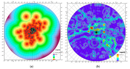
Figure 4.
(a) Analysis of water ice distances; (b) Kernel density analysis of the geologic map.
For the geological map, the quantitative results of the scientific element set were obtained using kernel density analysis, which was used to calculate the density of an element in its surrounding neighborhood. For the predicted density of (x,y) predicted points,
where i = 1, …, n are the input points. Only the points in the sum are included if they lie within a radius distance of the (x,y) location. popi is the value of the population field for point i, which is an optional parameter. disti is the distance between point i and the location (x,y). The calculated density is then multiplied by the number of points, or by the sum of the population fields, if any. This correction makes the spatial integral equal to the number of points (or the sum of the population field) rather than always equal to 1. This implementation uses a quadratic kernel. Separate equations need to be computed for each location where density is to be estimated. Since a raster is being created, the calculation will be applied to the center of each pixel in the output raster.
The formula used to determine the default search radius (also known as the bandwidth) is as follows:
Dm is the (weighted) median distance from the (weighted) center of the mean. n is the number of points for which the population field is not used, and n is the sum of the values of the population field if one is supplied. SD is the standard distance, which is computed as follows:
where xi, yi, and zi are the coordinates of element i denoting the mean center of the element, and N is equal to the total number of elements. The kernel density analysis of the geological map is shown in Figure 4b.
3.2.2. Working Mechanism of the SOM
The working process of the SOM can be divided into the following stages.
The SOM has a two-layer network structure. The input layer has n nodes corresponding to the n feature dimensions of the input samples. The output layer, also called the competition layer, has a node distribution that usually has a lower dimension (commonly two dimensions).
As can be seen from the learning process later, each node in the competitive layer is also represented by a feature vector of dimension. Therefore, each node can be regarded as a “clustering center”, and the learning process of the SOM is to map each input datum to a node in the competitive layer and to make closer the input data that are closer in the input space to the geometric position of the nodes in the competitive layer.
The number of nodes in the competitive layer determines the size of the SOM, which should have a sufficient number of nodes to ensure the accuracy and generalization ability of the model. An empirical formula for the minimum number of nodes that a 2D competitive network layer should have is given in the following equation:
where Nodesmin refers to the minimum number of nodes required for the network layer and n represents the number of input features.
Weight update: The weight vector of the node is updated using the following formula:
where wj(t) is the weight vector of node j, a(t) is the learning rate, hj,wc(t) is the neighborhood function, and x(t) is the input vector. As the number of training times increases, the learning rate and neighborhood radius gradually decrease, and the SOM network gradually converges, eventually forming a topological mapping to the input data.
3.2.3. Model Evaluation Parameters
The quantization error is a measure of the average of the distances between the input data points and their best-match units (BMUs). It reflects the accuracy of the SOM model’s representation of the input data. The smaller the quantization error, the more accurate the SOM model’s representation of the input data.
The topological error measures whether the BMUs and sub-BMUs (i.e., second closest neurons) of the input data points are neighbors. A smaller topological error indicates that the SOM network performs better in maintaining the topology of the data.
The contour coefficient is a metric used to assess the quality of clustering. It combines the distance of each data point from data points within the same cluster and its distance from the nearest other clustered data points. The contour coefficient can take values between −1 and 1. The larger the value, the more suitable the data point is for the cluster that it is in and the better the clustering effect. For any sample i in the dataset, the procedure for calculating the contour coefficient s(i) is as follows:
For the cluster distance (a(i)), for the sample i in the cluster C, calculate the average distance between i and all other points in C, which is written as a(i):
where d(i,j) denotes the distance between sample i and sample j.
Calculation of the inter-cluster distance (b(i)): For the cluster C where sample i is located, we calculate the average distance between i and all points in other clusters C′, denoted as b(i). Among all other clusters, we choose the smallest average distance b(i).
Calculation of the contour coefficient (s(i)): Based on the intra-cluster distance and inter-cluster distance, we calculate the contour coefficient of sample i.
The overall profile coefficient of the dataset is the average of all sample profile coefficients:
Contour coefficients close to 1 indicate good clustering, those close to 0 indicate that the data points lie on the boundary of two clusters, and negative values indicate that samples may be misclassified into the wrong cluster.
3.2.4. Bayes Optimization Approach in SOM Parameter Selection
In order to improve the performance of the SOM model, this study uses Bayesian optimization to optimize the key parameters of the SOM, including the learning rate, neighborhood radius, and the number of training iterations. Bayesian optimization approximates the objective function by constructing an agent model and using the model to select the next set of parameters, thus finding the optimal parameter combination within a limited number of evaluations.
Bayesian optimization is a global optimization method based on probabilistic models and is a strategy used for global optimization that is particularly suitable for optimizing computationally expensive black-box functions. Bayesian optimization finds the optimal solution in the least number of function evaluations by constructing an agent model (usually a Gaussian process or a tree-structured model), approximating the objective function, and using the agent model to select the next sampling point. The main steps include the following:
Surrogate model: Bayesian optimization uses a surrogate model to approximate the objective function f(x). The commonly used surrogate model is a Gaussian process.
A Gaussian process is a nonparametric Bayesian model used to define the prior distribution of the distribution function f(x). Suppose that the true value of the objective function f(x) is y; then,
where m(x) is the mean function and k(x, x′) is the covariance function. In the simple case, the mean function is usually set to zero, m(x) = 0. The covariance function usually uses a kernel function, the radial basis function:
where σf2 is the signal variance and l is the length scale. The next set of parameters is selected for evaluation by maximizing the expected improvement (EI) or other sampling strategies. A commonly used collection function is the expected improvement, which is defined as follows:
where x+ is the current optimal point. For specific calculations, assuming that the current optimum is f(x+), and the mean and variance at the new point x are μ(x) and σ(x), respectively, the expected improvement can be expressed as follows:
where Φ(Z) is the cumulative distribution function of the standard normal distribution, ϕ(Z) is the probability density function of the standard normal distribution, and ξ is a tuning parameter for balancing exploration and exploitation.
We set the objective function as follows: quantization error + topology error—profile coefficient.
Parameter update: We update the agent model using the results of the new evaluation and repeat the process until the stopping condition is satisfied.
Based on the training records of Bayesian hyperparameter optimization from Table 3 and Figure 5b, the optimal grid size is found to be 10, and the optimal number of iterations is 69.
Table 3.
Table of Bayesian hyperparametric optimization processes.
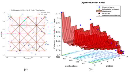
Figure 5.
(a) Schematic diagram of the SOM model. (b) Bayesian hyperparametric optimization graph.
3.2.5. Reordering of Clustering Centers
Since the classification results of the clustering model are unordered, for this specific problem of landing zone selection, it is possible to obtain classification results that meet the needs by reordering the clustering centers. For example, by arranging the clustering centers of each class of the slope data in a descending order, the first class of the classification results will have the lowest value for the slope, which is in line with the needs of landing engineering purposes.
3.2.6. Calculation of Feature Importance
Among the landing area selection considerations, the weight contribution of individual data to suitable landings is also of interest, and there is a lack of data-driven references for obtaining the weights of individual site selection element data in the landing site selection problem. However, the SOM method itself does not directly output how much each feature contributes to the classification results, as it is an unsupervised learning algorithm. The SOM helps to discover patterns or clustering structures in the data by mapping the data to a two-dimensional or low-dimensional space. The feature contribution can be indirectly obtained from the SOM model through a number of analytical methods. Thus, the importance of random forest features using machine learning can be indirectly obtained from the data weights by using the SOM clustering labels as classification targets and the features of the original input data as feature inputs to the model. A random forest is an integrated learning algorithm that classifies data by constructing multiple decision trees and, at the same time, is able to provide feature importance assessments. In this case, the random forest model can estimate the impact of each feature on the classification labels to obtain the importance weights of each siting data element on the classification results.
Feature importance assessment in random forests is based on the information gain (or reduction in impurity) calculated during node splitting, which reflects the importance of a feature in helping the decision tree to correctly classify it. When the decision tree is constructed, one feature at a time is selected to split the nodes, and this selection is based on the reduction in impurity (impurity). Impurity can be measured using Gini impurity or entropy. Suppose that there is a node t and the feature Xj. Xj is used to split the node into child nodes tL and tR, and then the reduction in impurity brought about by the feature can be expressed as follows:
where i(t) is the impurity of node t (e.g., Gini impurity or entropy).
NtL and NtR are the numbers of samples of the left and right child nodes.
Nt is the total number of samples of node t.
The importance of each feature can be measured using the cumulative reduction in impurity it induces in all trees:
That is, in all decision trees, the impurity reduction from each node split is part of the feature’s contribution to the final classification decision. Finally, the feature importance is normalized to between 0 and 1. The higher the feature importance, the higher the contribution of the feature to the classification result.
4. Results
The landing suitability evaluation results obtained using big data on the lunar polar region underwent a series of steps, including data resampling, vector data conversion, sliding window traversal, and SOM modeling. Next, the weight contribution of each type of data to the landing suitability was obtained using the characteristic importance method with a random forest; after that, the SOM evaluation results of the combined data were re-screened according to the principle of threshold selection, the results were categorized into two categories of suitable and unsuitable landing, and the results were compared with the South Pole landing sites selected by Zhang et al. [55]. These elements demonstrate the results of SOM landing zone preferences in the following three subsections: (1) lunar South Polar zone results for rating the suitability of landing zones with the SOM method, (2) landing assessment results from a data-driven perspective providing the weighted contribution of each site selection element and categorizing the combined data from the SOM evaluation results into two categories of suitable versus unsuitable landings by using the threshold filtering principle, and (3) superimposing the South Pole landing sites selected by Zhang et al. as well as preselected South Pole landing areas by various organizations to compare with the local areas of the integrated SOM results.
4.1. SOM-Based Evaluation of Lunar South Landing Zones
The SOM-based South Pole landing evaluation model integrates rich scientific data and engineering data and utilizes the sliding-window method for data slicing; the window sizes of 1° × 1°, 0.5° × 0.5°, and 0.03125° × 0.03125° are selected, and the step sizes in both directions are set to be 0.5°, 0.25°, and 0.015625°, respectively. The data are processed by the SOM model, and the clustering centers are reordered. The SOM evaluation results for the lunar polar region landing based on engineering data, scientific data, and comprehensive data are shown in Figure 6. In addition, 49 × 719, 99 × 1439, and 1599 × 23,039 landing suitability rating windows were obtained in the processing range of 65°S~90°S at the South Pole, respectively. The South Pole is superimposed with the center point of the Artemis 3 landing preselection area declared by NASA on 20 August 2022 (https://www.nasa.gov/news-release/nasa-provides-update-on-artemis-iii-moon-landing-regions/ (accessed on 28 October 2024)), as well as the preselected landing area centroids associated with South Pole landings by organizations collated in Table 1.
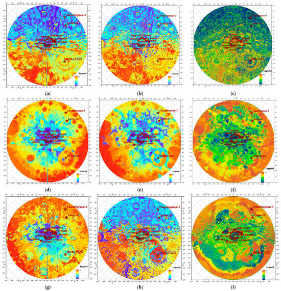
Figure 6.
SOM evaluation of lunar South Pole landing zones, where the legend represents the results of the categorization, blue represents the most suitable landing zones, and red represents the least suitable landing zones. The first through third rows represent engineering, scientific, and comprehensive evaluations, respectively. The first through third columns represent the evaluation results for the 1°, 0.5°, and 0.03° windows, respectively. (a) Engineering evaluation of the 1° window, (b) 0.5° window, (c) 0.03° window, (d) Scientific evaluation of the 1° window, (e) 0.5° window, (f) 0.03° window, (g) Comprehensive evaluation of the 1° window, (h) 0.5° window, and (i) 0.03° window.
Figure 6a–c provide an analysis of the conditions for landing in the South Polar region of the Moon based on engineering data and the SOM methodology. Among the rating metrics in the 100 categories of the legend, the results of category 1 indicate that it is the category with the lowest clustered central mean among the five categories of engineering data, thus representing the most suitable areas for landing, which have excellent performance in terms of light, communication, slope, and roughness, and are suitable for a future landing mission. The 100th category represents the category with the highest cluster-centered mean, which may be due to steep terrain, poor light conditions, or other unfavorable factors. The number of windows in the first through fifth categories that are most suitable for landing is 33,334,467, which is 9.05% of the total windows. The results demonstrate that factors such as illumination, communication, slope, and roughness combine to determine a window’s suitability for landing. Comparing Figure 3c, which shows the Earth visibility data in the polar region of the lunar South Pole, with the boundary from 90°W to 90°E, the data plot demonstrates a clear and gradual change in Earth visibility from high to low values from the upper to lower half of the boundary. In Figure 6a–c, containing the SOM results, most of the blue areas, which are suitable for landing, are distributed above the boundary, and the red areas, which are unsuitable for landing, are distributed below this boundary; this distribution feature is more obvious in the window sizes of 1° and 0.5°, which is consistent with the data distribution features for the Earth’s visibility. Comparing with Figure 3b, which shows the solar visibility data to indicate the lunar illumination, the boundary is from 90°W to 90°E. The impact craters above the boundary between 90°W and 90°E have lower illumination in the upper part of the crater wall, and the crater wall above the boundary is shown as a red range that is unsuitable for landing in the SOM result map; then, the area near the South Pole has lower illumination, and there are several permanently shaded areas, which are shown as unsuitable for landing in the SOM evaluation results with a small window size (0.03125°), which is in line with the illumination data. The area near the South Pole is shown as suitable for landing, but there is a contradiction in comparison with the illumination data, which is caused by the lower slope data and roughness data in the pole region that make it suitable for landing; therefore, the contribution of each data weight in the SOM results is also an issue to be considered. Comparing the data representing the lunar slope and roughness maps in Figure 3a,d–f, the bottoms of the impact craters within the study area are lower in terms of their slope and roughness values. Low values of slope and roughness at the bottom of an impact crater within the study area are also shown to be suitable for landing in the plot of the engineering results, while high values of slope and roughness at the wall portions of craters are shown to be unsuitable for landing relative to the bottom areas of craters in the plot of engineering results, which demonstrates a good correlation of the SOM results with the slope data and roughness data. Therefore, the polar region engineering landing evaluation results of the SOM absorb the distribution characteristics of each type of engineering data and are a comprehensive representation of the suitability of multidimensional engineering data for landing in the polar region, proving that the SOM method can integrate multidimensional data into a two-dimensional space, provide intuitive visualization results, and help decision makers to identify optimal regions quickly. In addition, the delineation of landing suitability is more refined as the window size decreases. Comparing the SOM engineering results in Figure 6a–c, the outline of the impact crater morphology in the polar region is clearer in Figure 6a–c. Comparing this with the Schrödinger Basin region declared by the HERACLES program, it is not suitable for landing when using the large window size, while it is suitable for landing when using the small window size due to the larger data values included in the model with the large window size and the higher values in the crater. This is due to the fact that the model contains more data values with the large window size, and the higher values in the edge portion of the impact crater affect the window mean. Therefore, the SOM results for the small window size (0.03125°) are better than those for the large window size when assessing the suitability of a polar region for landing.
Figure 6d–f provide an analysis of the conditions for landing in the South Polar region of the Moon based on scientific data and the SOM methodology, incorporating factors such as hydrogen content abundance, nuclear density analysis of geological maps, distance analysis of water ice, iron oxide abundance, and gravity anomalies. Of the 100 categories of rating metrics in the legend, the results in category 1 indicate that it is the category with the highest mean of the five scientific data clustering centers, representing the most suitable landing area that contains the highest scientific value. The number of windows in categories 1–5 of the most suitable landing areas containing the highest scientific value is 2,191,821, or 5.95%. The results demonstrate that, from a scientific point of view, the range suitable for landing is distributed in the region around the South Pole, which is consistent with the abundance of hydrogen content, the clustering of high values in geological maps and density analyses, and the distribution characteristics of water ice. The outlines of impact craters in the South Pole region in the SOM result maps are similar to those of the gravity anomaly data map, and the lower-left part of the boundary from 90°W to 90°E has a higher iron oxide content than the surrounding area. This is a similar feature to that seen in the SOM result map. The SOM result map also shows that the distribution of suitable areas for landing increases with decreasing latitude, which is consistent with the characteristics of the analysis of the distance to water ice. This feature is consistent with the analysis of water ice distances. Therefore, the scientific landing evaluation results of the SOM for the polar region have absorbed the distribution characteristics of each type of scientific data and are a comprehensive representation of the suitability of multidimensional scientific data for landing in the polar region.
Figure 6g–i provides a comprehensive analysis of conditions for landing in the South Polar region of the Moon based on engineering and scientific data using the SOM methodology, incorporating factors such as light, communication, slope, roughness, hydrogen content abundance, core density analysis of geological maps, distance analysis of water ice, iron oxide abundance, and gravity anomalies. Of the 100 categories of rating metrics in the legend, the results in category 1 represent the category with the most compatible landing conditions for the mean of the 10 engineering and scientific data clustering centers, representing the blue areas that are most suitable for landing. The number of windows for the most suitable landing areas in categories 1–5 is 1,872,531, or 5.08%. The green and yellow-green areas shown in the clustering results represent places with better-integrated conditions that are suitable as landing sites. The 18 existing landing site plans in Table 1 are clustered in these excellent areas except for the Shiv Shakti point landing site of Moon Ship III, which verifies the reliability of the SOM evaluation model. The Moon Ship III landing site near 69°S latitude has good engineering landing conditions, but it is far away from the permanently shaded area near the pole and has high values in the geological map kernel density analysis, and the low evaluation of its scientific value results in its unsuitability for landing. However, comparing the results of the SOM synthesis evaluation in Figure 6g with the data in Figure 6h, it can be seen that different conclusions are produced in the evaluation results with a window size of 1° versus 0.5°. Figure 6g demonstrates unsuitability for landing in the area above the boundary from 90°W to 90°E, and the general trend is similar to the characteristics of the SOM evaluation results for scientific data. Figure 6h demonstrates the suitability of landing in the area above the boundary from 90°W to 90°E, and the general trend is similar to the characteristics of the SOM evaluation results for engineering data. This contradiction may be caused by the following two reasons: 1. the weight contribution of each type of data in the SOM evaluation model is not consistent during the training process, which may cause a higher weight contribution of the scientific data to be shown in the SOM evaluation results, and therefore, it is necessary to analyze the data by obtaining the contribution of each type to the weights on the basis of that analysis. 2. From the perspective of meeting the landing conditions based on scientific and engineering data, there is a data conflict, and the overall trend is similar to that of the scientific data. There is a data conflict between the scientific data and the engineering data from the perspective of landing conditions. In permanently shaded areas, the higher hydrogen content abundance and water ice data are more suitable for landing because they reflect the scientific value of the area as a landing zone, but from the engineering point of view, there is very low light and communication, which is unsuitable for landing, so it is necessary to reclassify the clustering results of the SOM evaluation in order to alleviate this contradiction.
4.2. Weight Contributions of Multidimensional Features and Reclassification of the Synthesized Results
4.2.1. Weight Contributions of Multidimensional Features
Among the landing zone selection considerations, the weight contribution of individual data to suitable landings is also a matter of interest. For the SOM unsupervised learning algorithm, the feature contribution can be indirectly obtained from the SOM model through random forest special importance extraction. The SOM clustering labels are used as the classification targets, and the features of the original input data are used as the feature inputs to the random forest model. The weight contribution of each type of data within the target for engineering, scientific, and integrated landing objectives for suitable landing classification is shown in Figure 7.
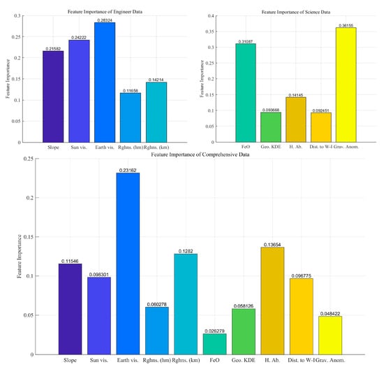
Figure 7.
Feature importance for the engineering, scientific, and comprehensive datasets.
In terms of the random forest feature importance results shown in Figure 7, the weighting of the influence of the characteristics of each type of engineering data (slope, light, communication, roughness, etc.) on site selection is analyzed as follows. Earth visibility (0.28324): The highest feature importance value in the figure is the most important engineering factor for a successful landing from a data-driven point of view, which is in line with the results of the South Pole SOM for the project in Figure 6c and is consistent with the conclusion that the characterization of the communication data is reflected. Stability of communications is associated with ensuring that the lander is able to communicate effectively with the Earth. Sun visibility (0.24222): Lighting conditions are the second most important feature, with sufficient sunlight helping to maintain the rover’s energy supply and ensure that the equipment operates properly in the harsh environment of the lunar South Pole. Slope (0.21582): The slope comes in a close second, indicating that the flatness of the terrain directly affects the safety of the lander’s landing. Lower slopes are beneficial in reducing the risk of the lander being in contact with the ground, thus reducing the likelihood of hard landings and capsizes. Roughness (km, 0.14214) and roughness (hm, 0.11658): Roughness is less important but still has some influence. Roughness reflects the smoothness of the surface and affects the stability of the lander’s landing. Earth visibility, Sun visibility, and slope are the main considerations in the current automated site selection, reflecting the priority of communication, energy supply, and the flatness of the surface of the landing zone in the engineering mission.
From the graph of the feature importance of scientific data, it can be seen that the contributions of scientific features for lunar South Pole landing site selection are as follows: Gravity anomalies (0.36155): Gravity anomalies have the highest feature importance in the scientific data, and the South Pole region is consistent with the conclusion that gravity anomalies characterize the data embodied in the results of the SOM evaluation in Figure 6c. This also suggests that gravity anomalies are the primary factor in automated site selection as scientific landing targets, as they are correlated with the internal structure of the Moon, geological activity, and topographic features, and can reveal hidden subsurface resources or inhomogeneous mass distributions, thus providing scientifically significant discoveries. FeO (0.31087): Iron oxide content follows closely, showing the importance of iron oxide abundance in scientific site selection. Areas of high iron oxide content hint at the presence of abundant metallic mineral resources on the Moon, which is important for future mineral extraction and resource utilization. Hydrogen abundance (0.14145): Hydrogen abundance is also a key scientific feature. The presence of hydrogen indicates the distribution of water ice, which in turn affects the detection of water resources on the Moon. Geo. KDE (0.093668) and Distance to W–I (0.092451): Geological kernel density estimation and the distance to the distribution of water ice are of low importance; geological maps reveal details of the Moon’s geological structure, and the distribution of the distance to water ice affects the ease of detecting direct evidence of water ice. Gravity anomalies, FeO, and hydrogen abundance are the main considerations in the current automated site selection for scientific landings, reflecting the prioritization of geological properties and resource potential in missions.
From the results of the feature importance analysis of the synthesized data, after combining the features of the engineering data and the scientific data, the feature importance was as follows: Earth visibility (0.23162): Communication remains the most important feature, showing that Earth visibility continues to be prioritized in ensuring communication between the lander and Earth. This is consistent with the needs of the engineering mission, where the reliability of communications is most important to mission success during the automated siting of the combined factors. Hydrogen abundance (0.13654): Hydrogen abundance became the second most important feature, indicating that the availability of water is critical for future missions in resource utilization and scientific exploration of the lunar South Pole. Roughness (km, 0.1282): Roughness increased in weight and is the third most important of the combined factors, which is related to the fact that roughness data at the kilometer scale not only affects landing safety but also reflects the bedrock geology as a feature for science. Slope (0.11546): The slope also has a higher weight and is an important factor in ensuring landing safety, especially for the lunar South Pole region, which has a more complex terrain. Sun visibility (0.098301) and distance to water ice (0.096775): Light and the distribution of the distance to water ice also carry considerable weight, indicating that ease of energy supply and access to resources were considered in site selection. FeO (0.060278): Iron oxide content decreased in importance but still reflects value in future mining and resource utilization. Geo. KDE (0.058126) and gravity anomalies (0.048422): The geological kernel density estimates and gravity anomalies have lower weights, but they provide information on geology and gravitational fields to provide complementary support for scientific exploration. In the synthesized data, communication (Earth visibility), hydrogen abundance, kilometer-scale roughness, and slope all have a weighting of more than 10% and are considered to be the four most important factors in the automated site selection process integrating scientific objectives and engineering needs. Of these, the kilometer-scale roughness data were slightly elevated in the combined weighting, consistent with the conclusion that these data reflect not only surface roughness from an engineering perspective but also bedrock geology from a scientific perspective [48].
4.2.2. Reclassification of the Consolidated Results
As mentioned in the previous section, there is a data conflict between the scientific data and the engineering data from the point of view of meeting the landing conditions; in permanently shaded areas, a higher hydrogen abundance and more water ice data are more reflective of the scientific value as a landing area and suitability for landing, but there is a very low illumination from the engineering point of view, which is unsuitable for landing, and the clustering results of the SOM evaluations need to be reclassified in order to alleviate this conflict. Specifically, for the clustering of composite conditions, the mean screening of cluster centers produces a disorder in the ordering of the classification results due to the conflict between the light data in engineering and the hydrogen content abundance and water ice distance data in science. Therefore, the principle of threshold screening was used to reclassify the results of the comprehensive SOM evaluation. To ensure a safe landing, fixed thresholds were determined for factors related to engineering safety: a slope less than 12°, solar visibility greater than 35%, and Earth visibility greater than 15%; this restriction meets the safety redundancy requirements in current Mars rover design [25,56]. Considering that exploration for water and other volatiles is the primary scientific objective, an elemental hydrogen abundance greater than 100 ppm was selected as the specific scientific limit [3,19].
The original clustering results of seven classes of all classifications satisfying this threshold condition were obtained, containing classes 1, 3, 21, 43, 47, 72, and 74, as the classification results for suitable landing, and they were superimposed on the preselected landing plan in Table 1, as well as 10 landing sites in four regions of the South Pole selected by Zhang et al. according to the engineering conditions. The WAC imagery maps were used as the base maps, with the blue areas as the suitable landing ranges after the screening of the integrated condition thresholds to obtain Figure 8.
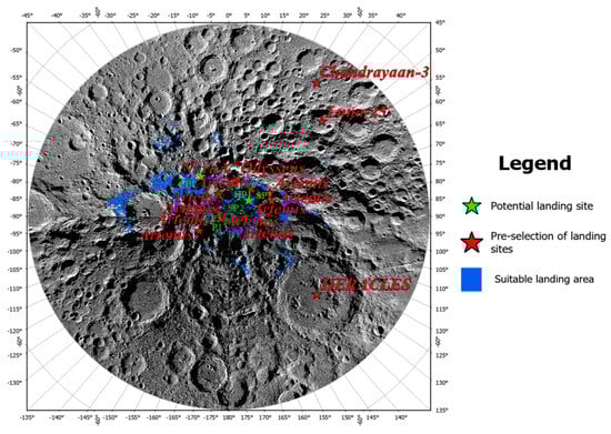
Figure 8.
Comprehensive SOM evaluation results based on threshold screening.
Figure 8 demonstrates the final classification of suitable ranges of landing zones based on the integrated data and the SOM methodology after the use of the threshold screening principle, after the zones were classified as suitable (blue) or unsuitable and then superimposed on the WAC image map, in combination with the display of landing sites and potential landing sites; thus, the distribution and selection of landing zones were visualized. This reflects the following characteristics: 1. The blue areas representing the most suitable landing zones in the integrated SOM evaluation results for the South Pole are mostly distributed near the poles; their distribution is similar to the characteristics of the range of hydrogen abundance of >100 ppm and similar to the characteristics of the SOM evaluation results for the scientific data. The number of blue windows suitable for landing is 2,457,515, accounting for 6.67% of the total. 2. Most of the blue areas suitable for landing are located on the rims of peaks, terraces, and ridges of craters, making them close to the permanently shaded impact craters, which is conducive to the discovery of the evidence of the presence of water ice and avoids the engineering limitation of the lack of light for the operation of detectors; in permanently shadowed areas, the tension between the scientific value of high hydrogen abundance and the technical requirements of weak illumination is partially eased. The edges of these impact crater peaks and ridges being identified as suitable landing areas is also consistent with the recommendation by Flahaut et al. [3] that small altitude increases using solar panels can significantly improve sunlight harvesting and provide a near-continuous power supply. 3 Since most South Pole exploration programs recommend suitable landing areas rather than landing sites, Zhang et al. [55] screened potential landing sites based on the principles of light conditions and local terrain flatness for comparison, and the results showed that all 10 potential landing sites in the four regions fell within the suitable landing range of the synthesized SOM results for the South Pole. The high overlap between the SOM results and the potential landing sites indicates that there is a high level of consistency between the existing scientific knowledge and the results of the SOM method, which also improves the reliability of the site selection model. This comprehensive analysis combines imagery, clustering results, and points from external authorities to show the most suitable areas for landing more clearly and provide a reference for practical operations. A local-area SOM evaluation at the South Pole in relation to an exploration program is specifically analyzed in the next section.
4.3. Regional Site Evaluation
After the above analysis of the SOM model results for the lunar South Pole, the localized areas associated with a South Pole exploration program can be given a recommended scope and in-depth analysis from a data-driven perspective. The following is an analysis of Zhang et al. and nine other regional scopes.
4.3.1. Malapert Massif
The Malapert Massif is a mountain range located south of the Malapert Crater (84.9S, 7.3E) at the lunar South Pole; it has a long sunshine period due to its high relief and is located on the edge of the inner ring of the SPA Basin [57]. It is considered one of the preferred locations for the Artemis III lunar exploration mission, as it contains a potential landing site.
The results in Figure 9 reflect the engineering, scientific, and comprehensive data and SOM landing suitability evaluations for the Malapert Massif, and they are analyzed as follows. 1. The SOM engineering evaluations show that the central part of the area is strip-shaped and suitable for landing, as it is located in the flat area of the mountain peaks, thus avoiding the higher slopes in the northern part and the roughness and low visibility of the illuminated Earth in the southern part. 2. The results of the scientific evaluation of the SOM of the region are similar to the characteristics of gravity anomalies in the region, which is consistent with the conclusion that the characteristics of gravity anomalies are the most important in the scientific SOM model. The relative proximity of the landing area to exposed water ice, as determined from the water ice distance data, increases the potential for scientific exploration of the area. 3. The combined results of the SOM evaluations show similar characteristics to the engineering data for the suitable landing range, with the central area being striped and suitable for landing, as it is located in a broadly flat area on the peak of the Malapert Massif, and with the HP1 potential landing site falling within the suitable landing range.
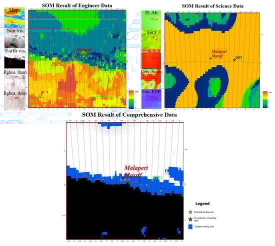
Figure 9.
Results of the SOM landing suitability evaluation of the Malapert Massif from three perspectives: engineering, scientific, and comprehensive perspectives.
Overall, the Malapert Massif region has excellent energy and communication conditions, with long periods of light helping to address the critical issue of energy supply, and due to the site’s high altitude, it can have almost direct visibility of the Earth, making it suitable for long-term exploration missions. In terms of scientific exploration, the region’s proximity to key scientific hotspots at the Moon’s South Pole could provide important support for future lunar resource development and scientific research.
4.3.2. Shackleton
The Shackleton impact crater, located at 89.7°S, 129.2°E, is 21 km in diameter, was formed during the Eratosthenian, and was excavated from an unconformity that exposed blocks containing probably the purest plagioclase on one side of the caldera and a layered outcrop on the other side of the caldera with a permanently shaded area of approximately 235 km2 in extent [13]. Layered outcrops on the other side of the crater contain a permanently shaded area of approximately 235 km2, which may be located in the inner ring of the SPA and, thus, demonstrate the deeper geology of the Shackleton crater and the South Pole of the Moon, and part of the crater rim (0.01 km2) is a permanently shaded area, and such a large permanently shaded area must have had a significant impact on the volatility of the moon [58]. It is a promising site for SPA investigations and water ice discovery near the South Pole. The nearby connecting ridge crater, which connects the Shackleton and Henson craters (known as the “connecting ridge” of the Artemis III potential landing zone) and the peak near Shackleton, is in permanent proximity to the center of the polar regions. This location is characterized by very specific geographic and environmental conditions. The extreme light conditions, temperatures, and topography of this location have made it a potential landing site in several lunar exploration and human lunar exploration programs, and it is considered one of the preferred sites for the Artemis III lunar exploration mission, with the region containing four potential landing sites.
The results in Figure 10 reflect the data and SOM landing suitability evaluation results for the Shackleton region from three perspectives: engineering, scientific, and synthesized. 1. The SOM engineering evaluation results show that there is a suitable landing range at the edge of the Shackleton crater location, and the connecting ridge location selected in the Artemis III mission falls into the suitable landing range. 2. The scientific SOM evaluation results in this region show that the scientific value of the Shackleton impact crater is higher than that of the surrounding area. 3. The combined results of the SOM evaluations show similar characteristics to the engineering data for suitable landing ranges, suggesting that the Shackleton edge and connect ridge are suitable for landing and that the four potential landing sites in the region, P1, P2, P3, and P4, fall within the suitable landing ranges.
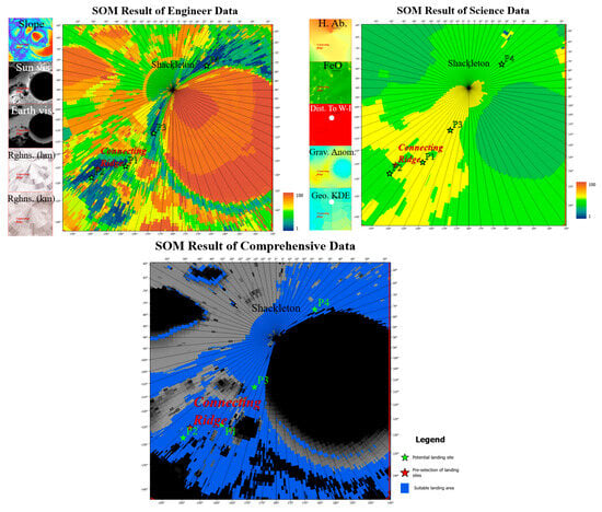
Figure 10.
Results of the SOM landing suitability evaluation of the Shackleton region from three perspectives: engineering, scientific, and comprehensive.
The results in Figure 11 reflect the data and SOM landing suitability evaluation results for the region of the peak near the Shackleton region from three perspectives: engineering, scientific, and synthesized. 1. The engineering SOM evaluation results show that the region of peak near Shackleton falls into a suitable landing range because of the gentle slope of the peak region, good illumination, and communication. 2. The scientific SOM evaluation results for this region show that the area near the peak has a higher scientific value than the surrounding area. 3. The synthesized SOM evaluation results show similar characteristics to those of the suitable landing range according to the engineering data, and it is concluded that there is a suitable landing range in and around the peak area. Overall, the Shackleton area is close to the permanently shaded area, is a priority impact crater for the detection of evidence of the presence of volatiles in the polar region, and has suitable conditions for engineering landings at the edge of the impact crater and on the connecting ridge. Despite the technical challenges of terrain and communications, its abundant water ice resources and unique polar environment offer great strategic value for long-term lunar exploration missions.
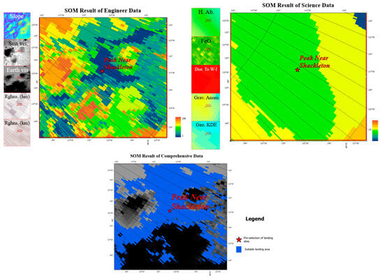
Figure 11.
Results of the SOM landing suitability evaluation for the peak near Shackleton from three perspectives: engineering, scientific, and comprehensive.
4.3.3. Haworth
Haworth Crater is a sub-pentagonal impact crater with a diameter of 35 km located in the South Polar region of the Moon. Approximately 4.76 km2 of the crater floor is permanently shadowed [58]. The Lunar Prospector neutron instrument detected hydrogen abundances of 142–144 ppm on the crater floor [37]. Thermal infrared (TIR) imaging indicates that the temperature at the bottom of the crater is very low, only 15–54 K (average temperature of 32–38 K), which allows for the long-term preservation of many volatiles, including water ice [11]. It is considered one of the preferred landing sites for the Artemis III mission, and it contains two potential landing sites.
The results in Figure 12 reflect the engineering, scientific, and integrated data and the SOM landing suitability evaluation of the Haworth region, and they are analyzed as follows. 1. The engineering SOM evaluation shows that the suitable landing area is distributed around the edge of the impact crater, avoiding the right part of the area with a high roughness and slope. 2. The characteristics of the scientific SOM evaluation are similar to the distribution of gravity data. 3. The comprehensive SOM evaluation results are similar to the characteristics of the engineering evaluation results, and the lower part of the comprehensive evaluation results has a wider range of suitable landing areas than the engineering results, which is caused by the higher values of the kernel density analysis (KDA) of the geological map in the lower part of the region, which absorbs the characteristics of the scientific data. In addition, the two potential landing sites in the region, CP2 and HP2, fall into the suitable landing range. Overall, the Haworth impact crater has been listed as one of the alternative landing sites by many international lunar exploration missions, and the rich resource potential of the region makes it a hotspot for international cooperation and research on lunar exploration and the utilization of lunar resources.
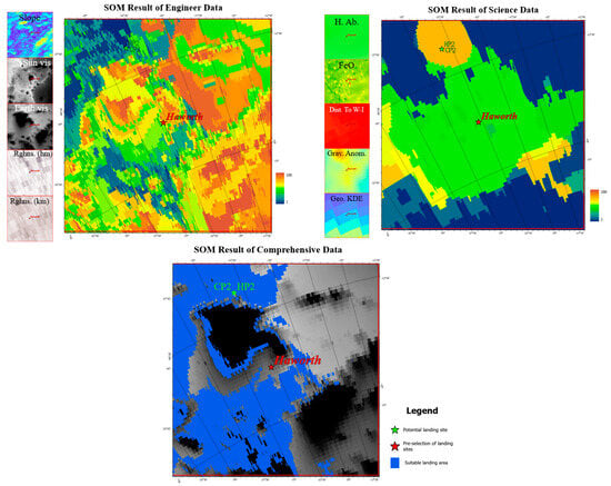
Figure 12.
Results of the SOM landing suitability evaluation in the Haworth from three perspectives: engineering, scientific, and comprehensive.
4.3.4. Cabeus
Cabeus Crater, located at 84.9°S 35.5°W, is an abraded formation with an average depth of 4 km at the base of the crater, a width of 60 km, and a slope of the crater wall of 10–15°. The crater is located at 84.9°S 35.5°W, and it has an average depth of 4 km at the base of the crater and a width of 60 km [59]. The temperature in the shadowed region is below 100 K (-173 °C), which would allow water ice to remain on or near the crater surface for billions of years without sublimating [60]. NASA’s LCROSS mission in 2009 successfully detected evidence of the presence of large amounts of water ice in the Cabeus crater. Water vapor and volatiles released by the impact further confirmed water ice reserves in the region, which contains one potential landing site.
The preselected landing area is located on the ridge north of the Cabeus impact crater. The results in Figure 13 reflect the data from three perspectives—engineering, scientific, and synthesized—and the results of the SOM landing suitability evaluation of the Cabeus region. 1. The engineering SOM evaluation results show a suitable landing area that is consistent with the low-slope ridge strike characteristics. 2. The characteristics of the scientific SOM evaluation results are similar to the characteristics of the gravity data distribution in the SOM, and the scientific value of the impact crater is higher than that of the ridge. 3. The comprehensive SOM evaluation results are similar to the engineering evaluation results; the potential landing site in the northern part of the Cabeus crater is close to it with a high scientific value, and the potential landing site CP1 falls into the range of suitable landings.
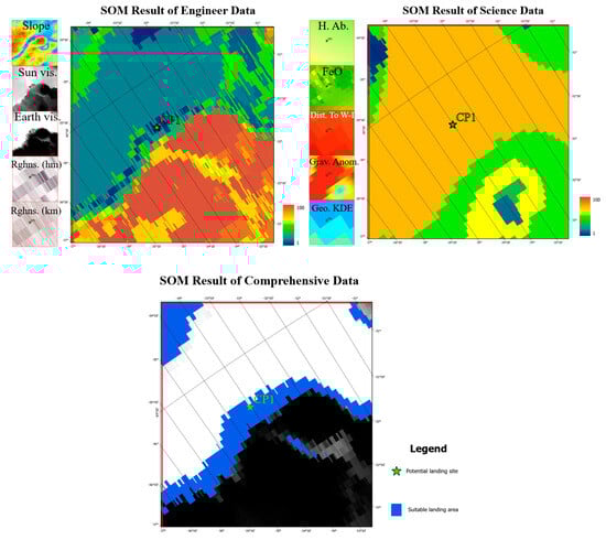
Figure 13.
Results of the SOM landing suitability evaluation for the Cabeus region from three perspectives: engineering, scientific, and comprehensive.
4.3.5. Shoemaker
Shoemaker Crater is located at 88.1°S, 44.9°E, with a diameter of about 51 km. Much of the crater floor is permanently shadowed, making it one of the largest permanently shadowed areas in the South Polar region of the Moon. A large number of impact spatter accumulations are distributed on the crater floor [61]. The hydrogen abundance at the bottom of the crater reaches 158–159 ppm. The temperature is very low, only 15–54 K (average temperature is 32–35 K), and this low temperature allows the long-term preservation of volatiles, including water ice, CO, CN, NH, etc.; therefore, it is one of the most probable areas on the Moon for the presence of a large number of volatiles of multiple types [11]. It contains the Nobile preselected landing area and potential landing site SP2.
The results in Figure 14 reflect the results of the potential landing site in the SP area according to the engineering and scientific data and the SOM landing suitability evaluation, and the following is the specific analysis. 1. The engineering SOM evaluation results show that SP2 is located at the edge of the impact crater, and the good slope, light, and communication conditions make this area suitable for landing, but the roughness is poor. 2. The scientific SOM evaluation results for this area show that the scientific value of the center area is higher than that of the edge area. 3. The comprehensive SOM evaluation results show that after combining the scientific features and engineering features, the edge area of the impact crater is considered suitable for landing, as it is conducive to safe landing and nearby detection. The potential landing site SP2 falls within the suitable landing range.
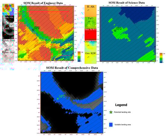
Figure 14.
Results of the SOM landing suitability evaluation for the Shoemaker region from three perspectives: engineering, scientific, and comprehensive.
The Rim 1 region of the Nobile impact crater is close to the South Pole of the Moon and is adjacent to the Shoemaker crater, and Figure 15 reflects the results of the engineering and scientific data and the SOM landing suitability evaluation of the Nobile Rim 1 region, which are analyzed as follows. 1. The engineering SOM results show that the ridges and highlands receive solar irradiation for a longer period of time, that the communication and topographic conditions are more favorable, and that the ridge region is suitable for landing. 2. The scientific SOM evaluation results in this region show that the center area of the impact crater has a higher scientific value than the ridge area. 3. The combined SOM results absorb the characteristics of the scientific and engineering results, and the ridge area is suitable for landing; there is also a suitable range of landing sites with suitable slopes in the low-lying area of the impact crater, and the potential landing site SP1 falls into the suitable landing range.
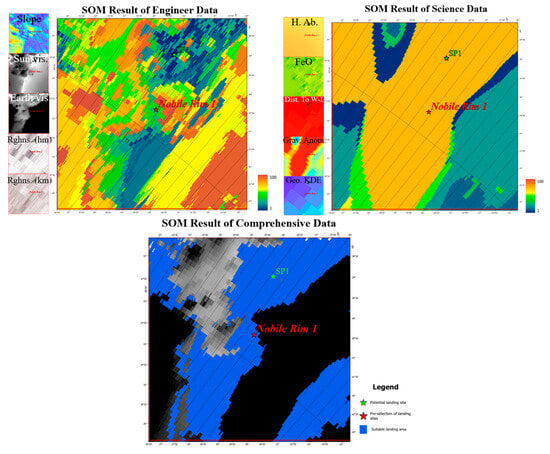
Figure 15.
Results of the SOM landing suitability evaluation for Nobile Rim 1 near the Shoemaker crater from three perspectives: engineering, scientific, and comprehensive.
4.3.6. Chandrayaan-3 and Luna-25 Landing Zone Assessment
The Chandrayaan-3 landing site is located in the South Polar region of the Moon, and Shiv Shakti Point is located between the lunar craters Manzinus C and Simpelius N at 69.373°S 32.319°E. A rover was repositioned by jumping and repositioning itself by 30–40 cm from the landing site. The Pragyan rover separated from the lander on 24 August 2023 and was surveyed in situ throughout the lunar day. Sulfur (S), aluminum (Al), calcium (Ca), manganese (Mn), ferrous (iron or ferrous), titanium (Ti), chromium (Cr), silicon (Si), and oxygen (O) were all successfully discovered by the rover. It also searched for hydrogen in the southernmost polar region of the Moon [17].
The results in Figure 16 reflect the results of the engineering and scientific data and the SOM landing suitability evaluation of the Shiv Shakti Point area, which are analyzed as follows: 1. The terrain in the area is relatively flat, with small slopes, which is conducive to a safe landing, and the lighting conditions meet the energy needs of landers, while the communication conditions are good for data transmission between Earth and the rover. The lighting conditions are good, as they meet the energy demands of the lander, and the communication conditions are also good, which is good for data transmission between the Earth and the rover. The engineering SOM results show that most of the area is suitable for landing, and there is already a landing site, Shiv Shakti Point, that falls into the range of suitability for landing. 2. This landing site is adjacent to the South Pole region of the Moon, which has potential for water ice exploration, and this is suitable for resource assessment and proximity. The results of the scientific SOM evaluation show that there is a range of outstanding scientific value in the vicinity of Shiv Shakti Point.
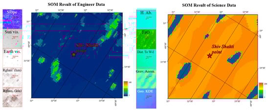
Figure 16.
Results of the SOM landing suitability evaluation for Shiv Shakti Point from the engineering and scientific perspectives.
The landing site of the Luna 25 is located at Guslavsky Crater in the South Polar region of the Moon at the coordinates 69.5°S, 43.5°E [62]. The maximum estimated mass fraction of water in the surface layer is 0.5%, suggesting the possible presence of water ice in the subsurface [63].
The results in Figure 17 reflect the results of the engineering and scientific data and the SOM landing suitability evaluation for the Boguslawsky region, and they are analyzed as follows. 1. The region has low relief, good lighting conditions, and good communications, and the engineering SOM results show that the Boguslawsky region contains a large area that is suitable for landing, and the preselected landing sites fall within the suitable landing range. 2. The results of the SOM scientific evaluation in this area show that there is a range of outstanding scientific interest to the east of Boguslawsky crater.
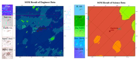
Figure 17.
Results of the SOM landing suitability evaluation for the Boguslawsky region from the engineering and scientific perspectives.
4.3.7. Summary of Regional Site Selection
Malapert Massif, with its high elevation, prolonged sunlight exposure, and excellent Earth visibility, has been identified as a preferred site for the Artemis III mission, making it suitable for long-term exploration missions. Its proximity to key scientific hotspots near the lunar South Pole further enhances its scientific exploration potential. Shackleton Crater, along with the nearby regions of the connecting ridge and peak near Shackleton, is a focal area for volatile detection due to its extensive permanently shadowed regions and extreme temperature conditions. Despite challenges related to terrain and communication, the area’s abundant water ice resources and unique environment offer significant strategic value for long-term lunar exploration. Haworth Crater, characterized by its low temperatures and high hydrogen abundance, has become a hotspot for international lunar missions. Suitable landing zones are primarily distributed along the crater’s edges, avoiding areas with high roughness and steep slopes. Cabeus Crater, known for its low-temperature environment and water ice deposits, which were confirmed by the LCROSS mission, is a critical area for scientific exploration. The proposed landing site on the northern ridge is close to the scientifically valuable crater floor. Shoemaker Crater and the adjacent Nobile Rim1 region, with their vast permanently shadowed areas and rich volatile potential, are ideal locations for detecting water ice and other volatiles. Suitable landing zones are mainly concentrated along the crater edges and ridges. The Shiv Shakti Point landing site of Chandrayaan-3, with its flat terrain, favorable illumination, and communication conditions, is well suited for safe landing and resource exploration, while its proximity to the lunar South Pole offers potential for water ice detection. The Boguslawsky Crater, selected for the Luna 25 mission, benefits from good illumination and communication conditions, as well as potential water ice resources, making it a prime area for scientific exploration. The proposed landing site is located on the eastern side, which exhibits high scientific value. Additionally, the 10 potential landing sites proposed by Zhang et al. all fall within suitable landing zones. Overall, the selection of these regions integrates both engineering considerations (such as slope, illumination, and communication) and scientific value (such as water ice resources and volatile detection), providing critical reference points for future lunar exploration missions.
5. Discussion
The application of the self-organizing mapping (SOM) method to the optimal selection of lunar South Pole landing zones is an efficient and innovative idea. The method downscales and visualizes multidimensional feature data (e.g., slope, illumination and communication conditions, surface roughness, hydrogen abundance, water ice resources, etc.) to help identify potentially preferable landing areas.
First, the SOM method has the risk of information loss when dealing with multidimensional data, especially in regions such as the lunar South Pole, with its complex terrain and uneven distribution of resources. Although the SOM method is able to demonstrate the clustering patterns of data through dimensionality reduction and visualization, due to the high dimensionality and complexity of the data, certain key features may be weakened or lost during the dimensionality reduction process, resulting in less accurate clustering results. Improvements can include introducing more advanced dimensionality reduction techniques to minimize the information loss and combining this with multi-source data fusion techniques to enhance the ability to capture key features.
Second, the SOM approach has limitations in feature importance analysis. Since the SOM method itself cannot directly provide the contribution of each feature to the clustering results, the feature importance needs to be indirectly assessed by introducing supervised learning models (e.g., with a random forest). However, this approach still cannot fully address the problem of complex relationships among features, especially when the weights of different features are inconsistent. Future improvements can explore combining deep learning models to more accurately reflect the relative importance between features through automatic feature extraction and weight assignment, thus enhancing the interpretability and reliability of clustering results.
Moreover, as an unsupervised method, SOM has the advantage of revealing inherent patterns and structures within the data without relying on pre-labeled ground truth. However, this does present limitations, as there is no direct validation of the identified “optimal” sites, and there is a potential risk of identifying landing sites that might be less optimal due to unmodeled hazards. For example, the SOM might group similar regions together based on the input features, but without ground truth data, we cannot fully verify whether these sites are truly optimal or if they contain hidden hazards (e.g., small craters, rocks, or uneven surface features) that were not captured in the input data. To mitigate this risk, future studies could involve cross-validation with known landing sites or integration of additional information from other sources, such as past mission data, high-resolution imagery, or field observations, to validate the suitability of the identified sites.
Finally, data quality and preprocessing have a significant impact on the clustering effect of the SOM method. Due to the inhomogeneity of data collection in the South Polar region of the Moon, feature data in some regions may be under-sampled, resulting in uneven spatial distribution of clustering results. In addition, the SOM method is sensitive to outliers, and normalization and denoising in data preprocessing are crucial. Improvements can include the development of more robust data preprocessing algorithms to minimize the interference of outliers and noise on the clustering results, and data enhancement techniques can be developed to compensate for the under-sampling problem so as to improve the applicability and stability of the SOM method in lunar South Pole landing zone selection.
Overall, the SOM method demonstrates great potential in lunar South Pole landing zone selection, but it still needs to be combined with more advanced data processing and analysis techniques to overcome its limitations and better support future lunar exploration missions.
6. Conclusions
The self-organizing mapping (SOM) method provides an effective means of clustering and visualizing multidimensional feature data during the selection of lunar South Pole landing zones. By downscaling data such as slope, light, communication conditions, roughness, hydrogen abundance, and water ice resources, the SOM method is able to identify potentially preferable areas that meet specific engineering and scientific needs. Combined with a supervised learning model such as a random forest, the clustering results of the SOM method are further analyzed to calculate the importance weights of each feature. This combined approach effectively compensates for the limitations of the SOM method in feature contribution analysis and allows for enhanced explanatory power and rationalization of landing zone selection, leading to the following conclusions.
1. The results of the engineering, scientific, and comprehensive SOM evaluation of the South Pole combined with 10 kinds of data were obtained, and the ranges of regions at the South Pole suitable for landing from engineering, scientific, and comprehensive perspectives accounted for 9.05%, 5.95%, and 5.08%, respectively.
2. The feature importance of each data point was weighted based on SOM automated site selection. In the engineering results, the weights from high to low were as follows: communication (0.28), light (0.24), slope (0.22), kilometer-scale roughness (0.14), and hectometer-scale roughness (0.12). In the scientific results, the weights from high to low were as follows: gravity anomaly (0.36), iron oxide (0.31), hydrogen abundance (0.14), geological map kernel density analysis (0.09), and water ice distance analysis (0.09). In the synthesized results, the weights were, in descending order, communication (0.23), hydrogen abundance (0.14), kilometer-scale roughness (0.13), slope (0.12), water ice distance analysis (0.10), light (0.10), hectometer-scale roughness (0.06), geological map kernel density analysis (0.06), gravity anomaly (0.05), and iron oxide (0.03). In the middle, the kilometer-scale roughness data were slightly elevated in the combined weights, which was consistent with the conclusion that these data reflect not only the surface roughness from the engineering point of view but also the bedrock geology from the scientific point of view [48].
3. Binary classification results of the South Pole landing suitability were obtained after threshold screening, and the results showed that 10 of the 10 preselected landing sites selected from Zhang et al. [55] fell within the suitable landing range, proving the effectiveness of the SOM model. Then, nine preselected landing zones were analyzed.
Although the SOM method has its challenges in scenarios with uneven data or complex correlations, its application in landing zone preselection shows good adaptability and provides reliable support for multi-feature integrated analysis for future lunar exploration missions. Through rational data preprocessing and adaptive screening methods, the SOM method can play an important role in the planning and resource assessment of lunar South Pole missions, providing a key reference for landing zone selection decisions.
Author Contributions
Conceptualization, Y.W. and H.L.; methodology, Y.W. and H.L.; software, H.L.; validation, S.W.; formal analysis, H.L. and S.W.; resources, S.Z.; data curation, J.L., K.Z. and S.Z.; writing—original draft preparation, H.L.; writing—review and editing, Y.W. and S.W.; visualization, H.L. and S.Z.; supervision, J.L. and K.Z.; project administration, Y.W.; funding acquisition, Y.W. All authors have read and agreed to the published version of the manuscript.
Funding
This research was funded by the National Key Research and Development Program of China (grant number: 2022YFF0503100).
Data Availability Statement
In this study, the WAC image data used in Figure 1 can be downloaded at: https://astrogeology.usgs.gov/search/map/moon_lro_lroc_wac_global_morphology_mosaic_100m (accessed on June 2013). The lunar South Pole remote sensing data used in Figure 2 can be found at the following locations: slope (Planetary Data System LOLA Data node (http://imbrium.mit.edu/EXTRAS/SLDEM2015/ (accessed on 24 January 2022))), Sun visibility and Earth visibility [9], roughness [48], FeO [49], hydrogen abundance [50], water ice exposure [38], geological map [52], and gravity [51].
Acknowledgments
The authors express their thanks to the people who helped with this study and the providers of the data used in this article, and they acknowledge the valuable suggestions from the peer reviewers.
Conflicts of Interest
The authors declare no conflicts of interest regarding the publication of this paper.
References
- Watson, K.; Murray, B.; Brown, H. On the possible presence of ice on the Moon. J. Geophys. Res. 1961, 66, 1598–1600. [Google Scholar] [CrossRef]
- Hayne, P.O.; Hendrix, A.; Sefton-Nash, E.; Siegler, M.A.; Lucey, P.G.; Retherford, K.D.; Williams, J.-P.; Greenhagen, B.T.; Paige, D.A. Evidence for exposed water ice in the Moon’s south polar regions from Lunar Reconnaissance Orbiter ultraviolet albedo and temperature measurements. Icarus 2015, 255, 58–69. [Google Scholar] [CrossRef]
- Flahaut, J.; Carpenter, J.; Williams, J.P.; Anand, M.; Crawford, I.A.; van Westrenen, W.; Füri, E.; Xiao, L.; Zhao, S. Regions of interest (ROI) for future exploration missions to the lunar South Pole. Planet. Space Sci. 2020, 180, 104750. [Google Scholar] [CrossRef]
- Lin, Y.; Tronche, E.J.; Steenstra, E.S.; van Westrenen, W. Evidence for an early wet Moon from experimental crystallization of the lunar magma ocean. Nat. Geosci. 2017, 10, 14–18. [Google Scholar] [CrossRef]
- Lin, Y.; van Westrenen, W. Isotopic evidence for volatile replenishment of the Moon during the Late Accretion. Natl. Sci. Rev. 2019, 6, 1247–1254. [Google Scholar] [CrossRef]
- Vasavada, A.R.; Paige, D.A.; Wood, S.E. Near-Surface Temperatures on Mercury and the Moon and the Stability of Polar Ice Deposits. Icarus 1999, 141, 179–193. [Google Scholar] [CrossRef]
- Mazarico, E.; Barker, M.K.; Jagge, A.M.; Britton, A.W.; Lawrence, S.J.; Bleacher, J.E.; Petro, N.E. Sunlit pathways between south pole sites of interest for lunar exploration. Acta Astronaut. 2023, 204, 49–57. [Google Scholar] [CrossRef]
- Gläser, P.; Oberst, J.; Neumann, G.A.; Mazarico, E.; Speyerer, E.J.; Robinson, M.S. Illumination conditions at the lunar poles: Implications for future exploration. Planet. Space Sci. 2018, 162, 170–178. [Google Scholar] [CrossRef]
- Mazarico, E.; Neumann, G.A.; Smith, D.E.; Zuber, M.T.; Torrence, M.H. Illumination conditions of the lunar polar regions using LOLA topography. Icarus 2011, 211, 1066–1081. [Google Scholar] [CrossRef]
- Flahaut, J.; Blanchette-Guertin, J.F.; Jilly, C.; Sharma, P.; Souchon, A.; van Westrenen, W.; Kring, D.A. Identification and characterization of science-rich landing sites for lunar lander missions using integrated remote sensing observations. Adv. Space Res. 2012, 50, 1647–1665. [Google Scholar] [CrossRef]
- Lemelin, M.; Blair, D.M.; Roberts, C.E.; Runyon, K.D.; Nowka, D.; Kring, D.A. High-priority lunar landing sites for in situ and sample return studies of polar volatiles. Planet. Space Sci. 2014, 101, 149–161. [Google Scholar] [CrossRef]
- Gawronska, A.J.; Barrett, N.; Boazman, S.J.; Gilmour, C.M.; Halim, S.H.; Harish; McCanaan, K.; Satyakumar, A.V.; Shah, J.; Meyer, H.M.; et al. Geologic context and potential EVA targets at the lunar south pole. Adv. Space Res. 2020, 66, 1247–1264. [Google Scholar] [CrossRef]
- Spudis, P.D.; Bussey, B.; Plescia, J.; Josset, J.-L.; Beauvivre, S. Geology of Shackleton Crater and the south pole of the Moon. Geophys. Res. Lett. 2008, 35, L14201. [Google Scholar] [CrossRef]
- NASA. NASA’s Plan for Sustained Lunar Exploration and Development. Available online: https://www.nasa.gov/sites/default/files/atoms/files/a_sustained_lunar_presence_nspc_report4220final.pdf (accessed on 6 April 2023).
- Fong, T.; Bluethmann, B.; Bridgwater, L. Overview of the Volatiles Investigating Polar Exploration Rover. In Proceedings of the Lunar Surface Innovation Consortium Meeting, Bowie, MD, USA, 31 August 2021. [Google Scholar]
- Hiesinger, H.; Landgraf, M.; Carey, W.; Karouji, Y.; Haltigin, T.; Osinski, G.; Mall, U.; Hashizume, K.; Heracles Science Working Group. HERACLES: An ESA-JAXA-CSA Joint Study on Returning to the Moon. In Proceedings of the 50th Lunar and Planetary Science Conference, Woodlands, TX, USA, 18–22 March 2019. [Google Scholar]
- Kanu, N.J.; Gupta, E.; Verma, G.C. An insight into India’s Moon mission—Chandrayan-3: The first nation to land on the southernmost polar region of the Moon. Planet. Space Sci. 2024, 242, 105864. [Google Scholar] [CrossRef]
- Kazmerchuk, P.V.; Shirshakov, A.E. The Luna-25 Spacecraft: Return to the Moon. Sol. Syst. Res. 2021, 55, 496–508. [Google Scholar] [CrossRef]
- Hu, T.; Yang, Z.; Li, M.; van der Bogert, C.H.; Kang, Z.; Xu, X.; Hiesinger, H. Possible sites for a Chinese International Lunar Research Station in the Lunar South Polar Region. Planet. Space Sci. 2023, 227, 105623. [Google Scholar] [CrossRef]
- Grant, J.A.; Golombek, M.P.; Wilson, S.A.; Farley, K.A.; Williford, K.H.; Chen, A. The science process for selecting the landing site for the 2020 Mars rover. Planet. Space Sci. 2018, 164, 106–126. [Google Scholar] [CrossRef]
- Turchinskaya, O.I.; Slyuta, E.N. Landing site choice for Luna-27 mission in the Moon South Polar Region. Acta Astronaut. 2024, 222, 346–358. [Google Scholar] [CrossRef]
- Golombek, M.P.; Grant, J.A.; Parker, T.J.; Kass, D.M.; Crisp, J.A.; Squyres, S.W.; Haldemann, A.F.C.; Adler, M.; Lee, W.J.; Bridges, N.T.; et al. Selection of the Mars Exploration Rover landing sites. J. Geophys. Res. Planets 2003, 108, 8072. [Google Scholar] [CrossRef]
- Zeng, X.; Mu, L. Lunar Spatial Environmental Indicators Dynamically Modeling Based Exploration Area Selection. Geomat. Inf. Sci. Wuhan Univ. 2017, 42, 91–96. [Google Scholar] [CrossRef]
- Wen, S.; Wang, Y.; Gong, Q.; Liu, J.; Kang, X.; Liu, H.; Chen, R.; Zhu, K.; Zhang, S. A New Robust Lunar Landing Selection Method Using the Bayesian Optimization of Extreme Gradient Boosting Model (BO-XGBoost). Remote Sens. 2024, 16, 3632. [Google Scholar] [CrossRef]
- Feng, Y.; Li, H.; Tong, X.; Li, P.; Wang, R.; Chen, S.; Xi, M.; Sun, J.; Wang, Y.; He, H.; et al. Optimized Landing Site Selection at the Lunar South Pole: A Convolutional Neural Network Approach. IEEE J. Sel. Top. Appl. Earth Obs. Remote Sens. 2024, 17, 10998–11015. [Google Scholar] [CrossRef]
- Liu, H.; Wang, Y.; Wen, S.; Liu, J.; Wang, J.; Cao, Y.; Meng, Z.; Zhang, Y. A New Blind Selection Approach for Lunar Landing Zones Based on Engineering Constraints Using Sliding Window. Remote Sens. 2023, 15, 3184. [Google Scholar] [CrossRef]
- Cao, Y.; Wang, Y.; Liu, J.; Zeng, X.; Wang, J. Selection of Whole-Moon Landing Zones Based on Weights of Evidence and Fractals. Remote Sens. 2022, 14, 4623. [Google Scholar] [CrossRef]
- Kohonen, T. The self-organizing map. Proc. IEEE 1990, 78, 1464–1480. [Google Scholar] [CrossRef]
- Wickramasinghe, C.S.; Amarasinghe, K.; Manic, M. Deep Self-Organizing Maps for Unsupervised Image Classification. IEEE Trans. Ind. Inform. 2019, 15, 5837–5845. [Google Scholar] [CrossRef]
- Bussey, D.B.J.; McGovern, J.A.; Spudis, P.D.; Neish, C.D.; Noda, H.; Ishihara, Y.; Sørensen, S.A. Illumination conditions of the south pole of the Moon derived using Kaguya topography. Icarus 2010, 208, 558–564. [Google Scholar] [CrossRef]
- De Rosa, D.; Bussey, B.; Cahill, J.T.; Lutz, T.; Crawford, I.A.; Hackwill, T.; van Gasselt, S.; Neukum, G.; Witte, L.; McGovern, A.; et al. Characterisation of potential landing sites for the European Space Agency’s Lunar Lander project. Planet. Space Sci. 2012, 74, 224–246. [Google Scholar] [CrossRef]
- Gläser, P.; Scholten, F.; De Rosa, D.; Marco Figuera, R.; Oberst, J.; Mazarico, E.; Neumann, G.A.; Robinson, M.S. Illumination conditions at the lunar south pole using high resolution Digital Terrain Models from LOLA. Icarus 2014, 243, 78–90. [Google Scholar] [CrossRef]
- McGovern, J.A.; Bussey, D.B.; Greenhagen, B.T.; Paige, D.A.; Cahill, J.T.S.; Spudis, P.D. Mapping and characterization of non-polar permanent shadows on the lunar surface. Icarus 2013, 223, 566–581. [Google Scholar] [CrossRef]
- Speyerer, E.J.; Robinson, M.S. Persistently illuminated regions at the lunar poles: Ideal sites for future exploration. Icarus 2013, 222, 122–136. [Google Scholar] [CrossRef]
- Zhang, J.A.; Paige, D.A. Cold-trapped organic compounds at the poles of the Moon and Mercury: Implications for origins. Geophys. Res. Lett. 2009, 36, L16203. [Google Scholar] [CrossRef]
- Paige, D.A.; Siegler, M.A.; Zhang, J.A.; Hayne, P.O.; Foote, E.J.; Bennett, K.A.; Vasavada, A.R.; Greenhagen, B.T.; Schofield, J.T.; McCleese, D.J.; et al. Diviner Lunar Radiometer Observations of Cold Traps in the Moon’s South Polar Region. Science 2010, 330, 479–482. [Google Scholar] [CrossRef]
- Fisher, E.A.; Lucey, P.G.; Lemelin, M.; Greenhagen, B.T.; Siegler, M.A.; Mazarico, E.; Aharonson, O.; Williams, J.-P.; Hayne, P.O.; Neumann, G.A.; et al. Evidence for surface water ice in the lunar polar regions using reflectance measurements from the Lunar Orbiter Laser Altimeter and temperature measurements from the Diviner Lunar Radiometer Experiment. Icarus 2017, 292, 74–85. [Google Scholar] [CrossRef]
- Li, S.; Lucey, P.G.; Milliken, R.E.; Hayne, P.O.; Fisher, E.; Williams, J.-P.; Hurley, D.M.; Elphic, R.C. Direct evidence of surface exposed water ice in the lunar polar regions. Proc. Natl. Acad. Sci. USA 2018, 115, 8907–8912. [Google Scholar] [CrossRef]
- Lawrence, D.J. A tale of two poles: Toward understanding the presence, distribution, and origin of volatiles at the polar regions of the Moon and Mercury. J. Geophys. Res. Planets 2017, 122, 21–52. [Google Scholar] [CrossRef]
- Sanin, A.B.; Mitrofanov, I.G.; Litvak, M.L.; Bakhtin, B.N.; Bodnarik, J.G.; Boynton, W.V.; Chin, G.; Evans, L.G.; Harshman, K.; Fedosov, F.; et al. Hydrogen distribution in the lunar polar regions. Icarus 2017, 283, 20–30. [Google Scholar] [CrossRef]
- Jawin, E.R.; Valencia, S.N.; Watkins, R.N.; Crowell, J.M.; Neal, C.R.; Schmidt, G. Lunar Science for Landed Missions Workshop Findings Report. Earth Space Sci. 2019, 6, 2–40. [Google Scholar] [CrossRef]
- Colaprete, A.; Schultz, P.; Heldmann, J.; Wooden, D.; Shirley, M.; Ennico, K.; Hermalyn, B.; Marshall, W.; Ricco, A.; Elphic, R.C.; et al. Detection of Water in the LCROSS Ejecta Plume. Science 2010, 330, 463–468. [Google Scholar] [CrossRef]
- Crawford, I.A. Lunar resources: A review. Prog. Phys. Geogr. Earth Environ. 2015, 39, 137–167. [Google Scholar] [CrossRef]
- Anand, M. Lunar Water: A Brief Review. Earth Moon Planets 2010, 107, 65–73. [Google Scholar] [CrossRef]
- Arnold, J.R. Ice in the lunar polar regions. J. Geophys. Res. Solid Earth 1979, 84, 5659–5668. [Google Scholar] [CrossRef]
- Smith, D.E.; Zuber, M.T.; Neumann, G.A.; Mazarico, E.; Lemoine, F.G.; Head Iii, J.W.; Lucey, P.G.; Aharonson, O.; Robinson, M.S.; Sun, X.; et al. Summary of the results from the lunar orbiter laser altimeter after seven years in lunar orbit. Icarus 2017, 283, 70–91. [Google Scholar] [CrossRef]
- Barker, M.K.; Mazarico, E.; Neumann, G.A.; Zuber, M.T.; Haruyama, J.; Smith, D.E. A new lunar digital elevation model from the Lunar Orbiter Laser Altimeter and SELENE Terrain Camera. Icarus 2016, 273, 346–355. [Google Scholar] [CrossRef]
- Kreslavsky, M.A.; Head, J.W.; Neumann, G.A.; Rosenburg, M.A.; Aharonson, O.; Smith, D.E.; Zuber, M.T. Lunar topographic roughness maps from Lunar Orbiter Laser Altimeter (LOLA) data: Scale dependence and correlation with geologic features and units. Icarus 2013, 226, 52–66. [Google Scholar] [CrossRef]
- Lemelin, M.; Lucey, P.G.; Camon, A. Compositional Maps of the Lunar Polar Regions Derived from the Kaguya Spectral Profiler and the Lunar Orbiter Laser Altimeter Data. Planet. Sci. J. 2022, 3, 63. [Google Scholar] [CrossRef]
- Lawrence, D.J.; Peplowski, P.N.; Wilson, J.T.; Elphic, R.C. Global Hydrogen Abundances on the Lunar Surface. J. Geophys. Res. Planets 2022, 127, e2022JE007197. [Google Scholar] [CrossRef]
- Lemoine, F.G.; Goossens, S.; Sabaka, T.J.; Nicholas, J.B.; Mazarico, E.; Rowlands, D.D.; Loomis, B.D.; Chinn, D.S.; Neumann, G.A.; Smith, D.E.; et al. GRGM900C: A degree 900 lunar gravity model from GRAIL primary and extended mission data. Geophys. Res. Lett. 2014, 41, 3382–3389. [Google Scholar] [CrossRef]
- Ji, J.; Guo, D.; Liu, J.; Chen, S.; Ling, Z.; Ding, X.; Han, K.; Chen, J.; Cheng, W.; Zhu, K.; et al. The 1:2,500,000-scale geologic map of the global Moon. Sci. Bull. 2022, 67, 1544–1548. [Google Scholar] [CrossRef]
- Ciazela, J.; Bakala, J.; Kowalinski, M.; Pieterek, B.; Steslicki, M.; Ciazela, M.; Paslawski, G.; Zalewska, N.; Sterczewski, L.; Szaforz, Z.; et al. Lunar ore geology and feasibility of ore mineral detection using a far-IR spectrometer. Front. Earth Sci. 2023, 11, 1190825. [Google Scholar] [CrossRef]
- Zwierzyński, A.J.; Ciążela, J.; Boroń, P.; Binkowska, W. Lunar Cold Microtraps as Future Source of Raw Materials—Business and Technological Perspective. Appl. Sci. 2023, 13, 3030. [Google Scholar] [CrossRef]
- Zhang, H.; Du, Y.; Li, F.; Zhang, H.; Ma, J.; Sheng, L.; Wu, K. Proposals for Sites Selection of Soft Landing on Lunar South Polar Region. J. Deep Space Explor. 2020, 7, 232–240. [Google Scholar] [CrossRef]
- Heldmann, J.L.; Colaprete, A.; Elphic, R.C.; Bussey, B.; McGovern, A.; Beyer, R.; Lees, D.; Deans, M. Site selection and traverse planning to support a lunar polar rover mission: A case study at Haworth Crater. Acta Astronaut. 2016, 127, 308–320. [Google Scholar] [CrossRef]
- James, P.B.; Smith, D.E.; Byrne, P.K.; Kendall, J.D.; Melosh, H.J.; Zuber, M.T. Deep Structure of the Lunar South Pole-Aitken Basin. Geophys. Res. Lett. 2019, 46, 5100–5106. [Google Scholar] [CrossRef]
- Xiao, L.; Qiao, L.; Xiao, Z.; Huang, Q.; He, Q.; Zhao, J.; Xue, Z.; Huang, J. Major scientific objectives and candidate landing sites suggested for future lunar explorations. Sci. Sin. Phys. Mech. Astron. 2016, 46, 29602. [Google Scholar] [CrossRef]
- Kozlova, E.A.; Lazarev, E.N. Crater Cabeus as Possible Cold Trap for Volatiles Near South Pole of the Moon. In Proceedings of the 41st Annual Lunar and Planetary Science Conference, The Woodlands, TX, USA, 1–5 March 2010; p. 1779. [Google Scholar]
- Feldman, W.C.; Maurice, S.; Lawrence, D.J.; Little, R.C.; Lawson, S.L.; Gasnault, O.; Wiens, R.C.; Barraclough, B.L.; Elphic, R.C.; Prettyman, T.H.; et al. Evidence for water ice near the lunar poles. J. Geophys. Res. Planets 2001, 106, 23231–23251. [Google Scholar] [CrossRef]
- Campbell, B.A.; Campbell, D.B. Regolith properties in the south polar region of the Moon from 70-cm radar polarimetry. Icarus 2006, 180, 1–7. [Google Scholar] [CrossRef]
- Djachkova, M.V.; Mitrofanov, I.G.; Sanin, A.B.; Litvak, M.L.; Tret’yakov, V.I. Characterization of the Luna-25 Landing Sites. Sol. Syst. Res. 2021, 55, 509–528. [Google Scholar] [CrossRef]
- Mitrofanov, I.G.; Zelenyi, L.M.; Tret’yakov, V.I.; Kalashnikov, D.V. Luna-25: The First Polar Mission to the Moon. Sol. Syst. Res. 2021, 55, 485–495. [Google Scholar] [CrossRef]
Disclaimer/Publisher’s Note: The statements, opinions and data contained in all publications are solely those of the individual author(s) and contributor(s) and not of MDPI and/or the editor(s). MDPI and/or the editor(s) disclaim responsibility for any injury to people or property resulting from any ideas, methods, instructions or products referred to in the content. |
© 2025 by the authors. Licensee MDPI, Basel, Switzerland. This article is an open access article distributed under the terms and conditions of the Creative Commons Attribution (CC BY) license (https://creativecommons.org/licenses/by/4.0/).