A Random Forest-Based Precipitation Detection Algorithm for FY-3C/3D MWTS2 over Oceanic Regions

Abstract

Satellite microwave-sounding radiometer data assimilation under clear-sky conditions typically requires the exclusion of precipitation-affected field-of-view (FOV) regions. However, the traditional scatter index (SI) and cloud liquid water path (CLWP)-based precipitation sounding algorithms from earlier NOAA microwave sounders are built on window channels which are not available from FY-3C/D MWTS-II. To address this limitation, this study establishes a nonlinear relationship between multispectral visible/infrared data from the FY-2F geostationary satellite and microwave sounding channels using an artificial intelligence (AI)-driven approach. The methodology involves three key steps: (1) The spatiotemporal integration of FY-2F VISSR-derived products with NOAA-19 AMSU-A microwave brightness temperatures was achieved through the GEO-LEO pixel fusion algorithm. (2) The fused observations were used as a training set and input into a random forest model. (3) The performance of the RF_SI method was evaluated by using individual cases and time series observations. Results demonstrate that the RF_SI method effectively captures the horizontal distribution of microwave scattering signals in deep convective systems. Compared with those of the NOAA-19 AMSU-A traditional SI and CLWP-based precipitation sounding algorithms, the accuracy and sounding rate of the RF_SI method exceed 94% and 92%, respectively, and the error rate is less than 3%. Also, the RF_SI method exhibits consistent performance across diverse temporal and spatial domains, highlighting its robustness for cross-platform precipitation screening in microwave data assimilation.

1. Introduction

In recent years, satellite microwave sounding data, which are represented by Advanced TIROS Operational Vertical Sounder (ATOVS) radiance measurements, have gradually become one of the main data sources for numerical weather prediction centers, such as the European Center for Medium-term Numerical Prediction (ECMWF) and the National Environmental Prediction Center (NCEP) in the United States. Microwave detection has the advantage of providing information concerning the atmospheric thermal structures of nonprecipitation cloud regions, which cover approximately 70% of the Earth’s surface. Therefore, identifying precipitation-contaminated pixels is essential for effective microwave data assimilation.

The detection of microwave precipitation significantly influences the microwave sounding data assimilation’s effectiveness [1]. On the one hand, strong scattering by large hydrometeors attenuates microwave penetration through precipitating clouds. On the other hand, microwave scattering is highly nonlinear and thus cannot be accurately simulated by the linearized forward algorithm operator in assimilation systems [2]. Therefore, before clear-sky microwave satellite data are assimilated, pixels contaminated by precipitation must be removed. Current operational precipitation detection methods for microwave temperature sounders utilize brightness temperature differences across the 23-, 31-, and 89-GHz channels to compute the scatter index (SI), which determines precipitation intensity over land surfaces [3] and on the ocean surface [4]. Weng et al. [5] used cloud liquid water retrieved from the brightness temperature data in the 23- and 31-GHz channels as a microwave scattering signature, which is widely performed in gridpoint statistical interpolation (GSI) assimilation systems.

However, the Microwave Temperature Sounder II (MWTS2) onboard the FY-3C/D satellite, which has a nadir spatial resolution of 33 km, lacks the 23-, 31-, and 89-GHz channels required for precipitation detection [6,7]. Therefore, the traditional microwave precipitation detection algorithms are no longer applicable to these microwave instruments. Li and Zou [8] developed a new precipitation detection scheme by matching visible and infrared radiometer (VIRR)/medium-resolution spectral imager (MERSI) cloud mask data with MWTS2 pixels and used the matched cloud fraction as an alternative to the traditional method employed for MWTS2 data. This method treats clouds as integrated systems, accounting for microphysical processes to infer precipitation from cloud-top imager data [9]. Eventually, the assimilation of MWTS2 observation data is achieved, which makes a positive contribution to the global forecasts of the Global/Regional Assimilation and Prediction System (GRAPES) [10]. Sun and Fu [9] combined Tropical Rainfall Measuring Mission (TRMM) precipitation radar (PR) and Visible Infrared Scanner (VIRS) data with ERA5 reanalysis to analyze cloud/precipitation interactions in a case study.

Recent advancements in artificial intelligence have spurred growing interest in its application to satellite-based precipitation detection. However, most existing machine learning models remain “black-box” systems, limiting mechanistic insights into precipitation processes and hindering model interpretability. Notably, the random forest (RF) algorithm stands out as one of the few interpretable machine learning models, leveraging the Gini importance index to quantitatively evaluate feature contributions. This capability has driven its successful adoption in satellite-based precipitation detection. For instance, Zhang et al. demonstrated the effectiveness of integrating precipitation zoning with RF regression for spatial downscaling of satellite rainfall estimates in the Lancang–Mekong River Basin [11]. Wang et al. employed RF regression with FY-4A satellite infrared brightness temperatures to improve precipitation estimation accuracy [12], while Chen et al. proposed an RF-based downscaling-calibration method that outperformed classical approaches like geographically weighted regression and artificial neural networks in generating high-resolution precipitation datasets [13]. Nguyen et al. further validated RF’s superiority over traditional statistical fusion methods through multi-source satellite precipitation integration in South Korea [14]. Kühnlein et al. [15] applied the random forest algorithm to precipitation prediction, which improved the accuracy of the precipitation rate determined by optical satellite sensors.

To enable more accurate and efficient precipitation detection for MWTS2 and provide a novel precipitation detection approach for future MWTS2 data assimilation, this paper proposes a new precipitation detection method (denoted as RF_SI) by using fused FY-2F VISSR and NOAA-19 AMSU-A data as a training dataset in combination with the random forest model employed in machine learning approaches. Compared with conventional imager-matched MWTS2 precipitation algorithms, the RF_SI method, which uses more cloud parameters (the relative humidity, cloud classification, cloud-top temperature, and water vapor values in the middle and upper levels of the troposphere), can accurately simulate the nonlinear relationships between cloud parameters and microwave precipitation signals with a higher spatiotemporal resolution. RF_SI information can be matched with MWTS2 pixels to assist MWTS2 in performing precipitation detection. This paper focuses on the precipitation detection principle of RF_SI and evaluates its precipitation detection effect. In the future work, we plan to implement the RF_SI method in MWTS2 data assimilation systems to further validate and operationalize this approach.

The remainder of this paper is organized as follows. Section 2 introduces the satellite data, the GEO-LEO satellite pixel fusion algorithm, and the multispectral microwave precipitation identification method developed based on the random forest approach. The preprocessing method applied to the given machine learning datasets and the model training process are described in Section 3. Section 4 presents the experimental and analysis results obtained for a single case and a long-term series case by using the FY-2F satellite cloud products. Finally, a summary and a conclusion are given in Section 5.

2. Data and Methods

The methodological diagram of this paper, as shown in Figure 1, is divided into three interconnected components. Part 1 focuses on the generation of a machine learning training dataset through multi-source data fusion. Specifically, Level 2 cloud products derived from VISSR (5 km resolution) and SI of AMSU-A (45 km resolution) are integrated using the pixel fusion algorithm, producing a unified training and test dataset for subsequent model training.

Part 2 outlines the training phase of the random forest algorithm. The fused dataset undergoes preprocessing to ensure compatibility and quality, followed by iterative training to optimize the model parameters. The output of this stage is a trained RF model capable of simulating the RF_SI, a critical metric for precipitation prediction.

Part 3 details the validation and inference workflow. Independent validation data, including VISSR L2 cloud products, are fed into the trained RF model to generate simulated RF_SI values. A threshold-based decision mechanism is applied, where RF_SI values exceeding 30 trigger a “Precipitation” classification, while values below this threshold result in a “No Precipitation” outcome.

2.1. Satellite Microwave Radiometer

2.1.1. Advanced Microwave Sounding Unit-A (AMSU-A)

The NOAA-19 polar-orbiting meteorological satellite is the fifth operational polar-orbiting meteorological satellite in the ATOVS series launched by the NOAA, with an orbital altitude of approximately 870 km, an inclination angle of 98.9°, and a period of 101.4 min. The onboard AMSU-A is a 15-channel microwave radiometer that was designed for profiling atmospheric temperatures in the 50–60 GHz atmospheric oxygen absorption band and has detection channels in the 23.8-, 31.2-, and 89-GHz atmospheric window areas for precipitation identification purposes. The AMSU-A instrument adopts a cross-track scanning strategy, with each scanning line containing 30 detection pixels. The imaging resolution at the subsatellite point is 45 km, and the width of each scanning line is approximately 2200 km. The scanning angle corresponding to the orbital edge pixels is 55.4°. Since the first AMSU-A was launched on NOAA-15 in 1998, AMSU-A and its subsequent ATMS observations have become among the most influential data sources for numerical weather prediction [16].

Clouds are essentially black bodies relative to the infrared band in terms of their radiation, and they strongly absorb infrared radiation. Infrared (IR) sensors predominantly capture information from cloud-top surfaces, which makes reflecting the internal precipitation information contained within cloud bodies difficult. In contrast, microwaves, with their longer wavelengths, can penetrate clouds to a certain extent and detect precipitation information within cloud bodies. Hence, the AMSU-A satellite microwave thermometer is chosen as the training set for precipitation detection.

The indicator that reflects the scattering effect of AMSU-A caused by precipitation and other factors is usually represented by the SI, which is selected as the label for the training dataset in this paper:

$$SI=ETB15-TB15$$

(1)

$$ETB15=a+bTB1+cTB2+dTB3$$

(2)

where SI is the scatter index; TB1, TB2, TB3, and TB15 are the brightness temperatures of AMSU-A channels 1 (23.8 GHz), 2 (31.4 GHz), 3 (50.3 GHz), and 15 (89.0 GHz), respectively; ETB15 is the simulated clear-sky brightness temperature of channel 15; and a, b, c, and d are tangent polynomials that describe the scanning angles. The SI is crucial for enhancing the efficiency of microwave observation data utilization and has a significant effect on numerical weather prediction.

In addition to the SI, this study selects the cloud liquid water path (CLWP) as a diagnostic criterion for precipitation detection, which can be expressed as follows:

$$CLWP=\cos (local\_zenith)\ast (a+0.754log(285-TB1))-2.265\log (285-TB2)$$

(3)

$$a=8.240-(2.622-1.846\ast \cos (local\_zenith))\ast \cos (local\_zenith)$$

(4)

where CLWP is the cloud water path, local_zenith is the zenith angle of the satellite, and TB1 and TB2 are the brightness temperatures of channels 1 and 2, respectively. When the CLWP is greater than 0.5 g/kg [17], precipitation is considered to have occurred.

2.1.2. Microwave Temperature Sounder (MWTS)

The MWTS is divided into two generations: MWTS2, which is mounted on the FY-3C/D satellites, and MWTS3, which is mounted on FY-3E.

Table 1. MWTS2 and MWTS3 channel characteristics.

Channel Index		Center Frequency (GHz)		Polarization		Main Purpose
MTWS3	MWTS2	MTWS3	MWTS2	MTWS3	MWTS2	MTWS3	MWTS2
1		23.80		QH		Cloud and Precipitation
2		31.40		QH		Cloud and Precipitation
3	1	50.30	50.30	QV	QH	Temperature	Temperature
4	2	51.76	51.76	QV	QH	Temperature	Temperature
5	3	52.80	52.80	QV	QH	Temperature	Temperature
6		53.246 ± 0.08		QV		Temperature
7	4	53.596 ± 0.115	53.596	QV	QH	Temperature	Temperature
8		53.948 ± 0.081		QV		Temperature
9	5	54.40	54.40	QV	QH	Temperature	Temperature
10	6	54.94	54.94	QV	QH	Temperature	Temperature
11	7	55.50	55.50	QV	QH	Temperature	Temperature
12	8	57.290344 (fo)	57.290344 (fo)	QV	QH	Temperature	Temperature
13	9	fo ± 0.217	fo ± 0.217	QV	QH	Temperature	Temperature
14	10	fo ± 0.3222 ± 0.048	fo ± 0.3222 ± 0.048	QV	QH	Temperature	Temperature
15	11	fo ± 0.3222 ± 0.022	fo ± 0.3222 ± 0.022	QV	QH	Temperature	Temperature
16	12	fo ± 0.3222 ± 0.010	fo ± 0.3222 ± 0.010	QV	QH	Temperature	Temperature
17	13	fo ± 0.3222 ± 0.0045	fo ± 0.3222 ± 0.0045	QV	QH	Temperature	Temperature

presents the characteristics of the MWTS channels.

MWTS2 is a cross-track scanner that completes one revolution every 8/3 s, scans 90 Earth FOVs with a 33 km nadir resolution, and measures Earth’s radiation across 13 channels from 50 to 60 GHz for temperature profiling from the surface to approximately 6 hPa. Owing to the limitations imposed by early industrial technology, China’s MWTS2 has consistently lacked a low-frequency microwave precipitation detection channel, such as one at 23 or 31 GHz, which is necessary for calculating the SI or CLWP to complete precipitation detection tasks.

In contrast with MWTS2, the MWTS3 system has been enhanced with the inclusion of 23.8-GHz and 31.4-GHz channels, which were specifically designed for the detection of clouds and precipitation. MWTS3 is capable of estimating the CLWP by utilizing measurements acquired from both the 23.8-GHz and 31.4-GHz channels.

To evaluate the applicability of RF_SI to MWTS2, the RF_SI data introduced in this paper can be matched within the MWTS3 pixels. A comparative analysis of the precipitation detection results produced by the RF_SI and CLWP schemes can subsequently be performed.

2.2. Visible and Infrared Spin Scan Radiometer (VISSR)

The Fengyun-2 (FY-2) meteorological satellite is a first-generation geostationary meteorological satellite developed in China. It can acquire daylight-visible cloud maps, day–night infrared cloud maps, and water vapor distribution maps with a high frequency. The VISSR is a visible/near-infrared scanning radiometer mounted on FY-2 that consists of one visible-band channel (0.55–0.99 μm) and four infrared bands (3.50–4.00 μm, 6.30–7.60 μm, 10.3–11.3 μm, and 11.5–12.5 μm). The VISSR completes full-disk images consisting of 2288 × 2288 pixels every hour, with substellar point resolutions of 5 km (infrared) and 1.25 km (visible/near-infrared) [18]. FY-2F is the sixth satellite in the FY-2 series and was launched on 13 January 2012; it orbits over the equator at 112°E. The meteorological satellite and polar-orbiting meteorological satellite of FY-2 complement each other and constitute the application system of China’s meteorological satellite.

Based on the observational data provided by the VISSR, real-time cloud images and dozens of retrieval products, such as clear-sky atmospheric radiation, atmospheric motion vectors, and sand–dust images, can be obtained. The cloud data retrieved from the FY-2F VISSR and used in this paper are shown in Figure 2, including the relative humidity profile (HPF) for 300–1000 hPa, the cloud classification results (CLC, with a total of 7 types: clear-sky sea surfaces, hybrid cells, high-level clouds, cirrocumulus clouds, dense stratus clouds, cumulonimbus clouds, and stratocumulus clouds), the water vapor content in the upper tropospheric humidity (UTH), and the cloud-top temperature (CTT).

The FY-2F VISSR product and the FY-3E MWTS3 and NOAA-19 AMSU-A observations used in the experiments are obtained from the National Satellite Meteorological Center: http://www.nsmc.org.cn/nsmc/cn/home/index.html (accessed on 14 April 2025).

2.3. GEO-LEO Satellite Image Fusion Algorithm

The FY-2F satellite has a geostationary orbit, whereas NOAA-19 has a sun-synchronous orbit. The optical paths and observation time of the VISSR and AMSU-A modules onboard these two different satellites for the same target are not exactly the same, and the projections of their detection pixels on the ground are also different. To make the observations of the VISSR and AMSU-A more comparable, the VISSR pixels and AMSU-A pixels are also paired; that is, they are matched to the same pixels and share the same observation time within a certain threshold range.

2.3.1. Time Matching

$$\left|t_{VISSR}-t_{AMSU-A}\right|<{\mathit{\delta }}_{\max \_min}$$

(5)

where t_VISSR indicates the observation time of the VISSR pixel, t_AMSU-A represents the observation time of the AMSU-A pixel, and δ_{max_min} is the time threshold. When the observation time difference between the VISSR and AMSU-A data is less than the empirical threshold δ_{max_min}, we consider the two observations to be “simultaneous observations”. In this paper, δ_{max_min} is 30 min.

2.3.2. Observed Object Matching

Only if the study region is near the equator can the optical path difference caused by the different observation zenith angles and azimuth angles of the VISSR and AMSU-A be ignored. The remaining regions require the intercalibration of geostationary and polar-orbiting satellite sensors [19], as expressed in (6), to ensure the consistency of the observation objects:

$$\left|{\displaystyle \frac{\cos {\mathit{\theta }}_{LEO}}{\cos {\mathit{\theta }}_{GEO}}}-1\right|<\mathit{\alpha }$$

(6)

where θ_LEO is the zenith angle of a polar-orbiting satellite, θ_GEO represents the zenith angle of a geostationary satellite, and α is an empirically determined threshold. If the difference between the zenith angles of the two satellites is less than the empirical threshold α = 0.08, the objects observed by the two sensors onboard can be considered the same. Thus, when the difference between the zenith angles of the VISSR and AMSU-A satisfies (6), a matching sample is selected.

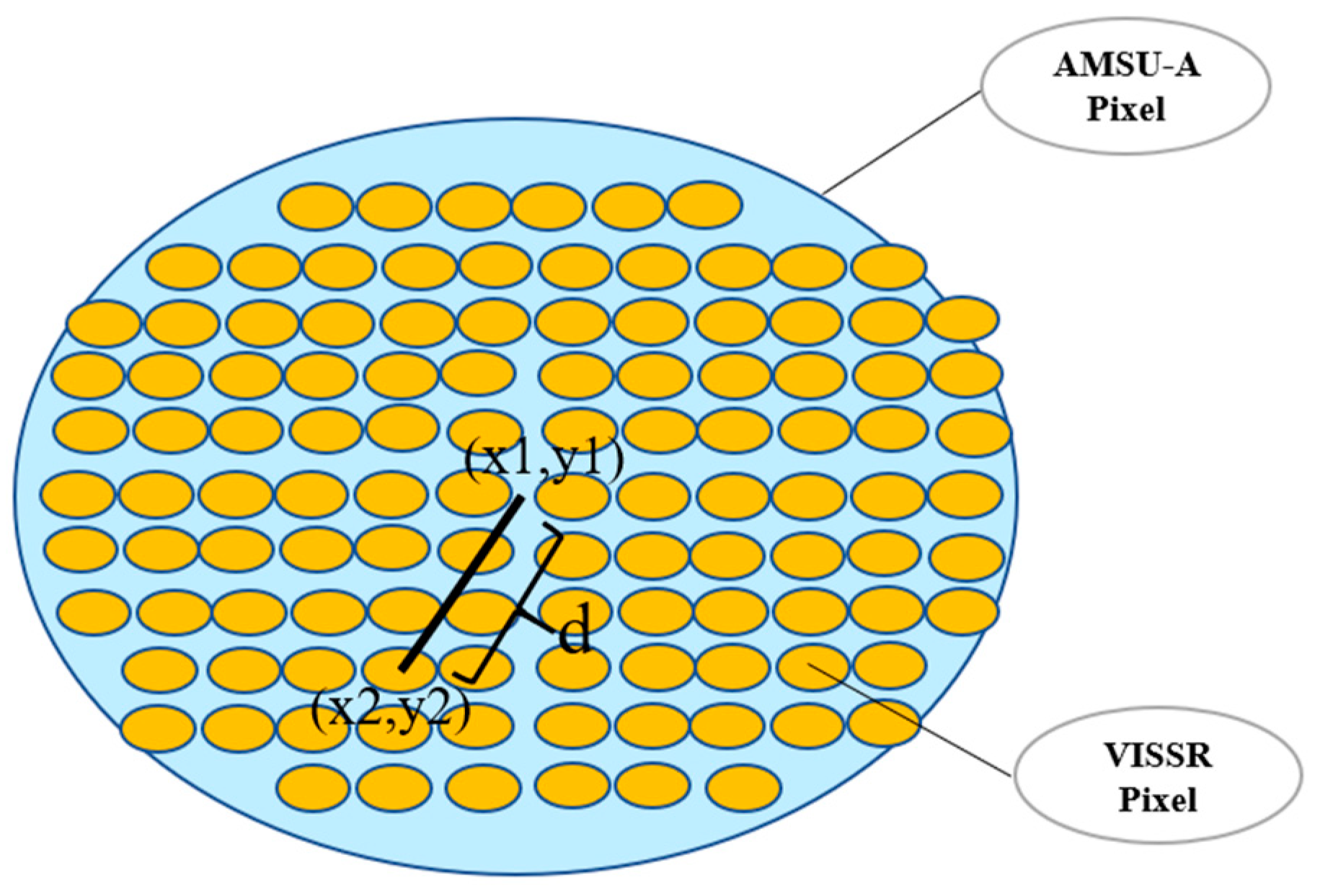
2.3.3. Pixel Matching

The physical products of the VISSR are the input features, and AMSU-A provides the SI as a machine learning label. We need to fuse the VISSR and AMSU-A pixels to construct training sets. The spatial resolution of the AMSU-A pixels (45 km) is much lower than that of the VISSR pixels (5 km), and the pixel deformation caused by the Earth’s curvature is ignored under the constraints of the zenith angle of the satellite. When the center distance between two pixels is less than the empirical distance threshold dmax, a VISSR pixel is considered an AMSU-A pixel in the footprint [20].

$$d=2R{\sin }^{-1}\sqrt{{(\sin {\displaystyle \frac{x2-x1}{2}})}^2+\cos x1\ast \cos x2\ast {(\sin {\displaystyle \frac{y2-y1}{2}})}^2}$$

(7)

$$d<d_{\max }$$

(8)

where x1 and y1 are the latitude and longitude of the AMSU-A pixel, respectively; x2 and y2 represent the latitude and longitude of the VISSR data, respectively; R is the radius of the Earth; and dmax is set as a threshold of 30 km. After the VISSR pixels within the AMSU-A footprint that satisfied the distance criteria are identified, the average value of these VISSR pixels is utilized as input information. The schematic diagram of the pixel-matching process is shown in Figure 3.

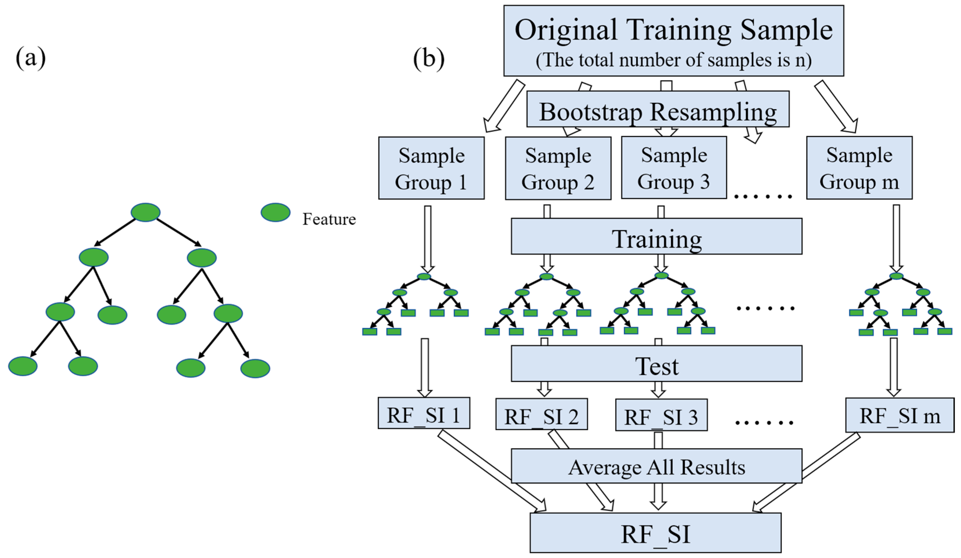
2.4. Precipitation Identification Method Based on the Random Forest Algorithm

The random forest algorithm is an ensemble learning method based on decision trees. First proposed by Breiman [19] in 2001, the random forest algorithm combines the bagging-based ensemble learning algorithm [21] with a random subspace [22], which can naturally model nonlinear decision boundaries and thus effectively solve nonlinear problems. The basic building blocks of the random forest model are decision trees, and the decision trees used in this paper are classification and regression trees (CARTs) [23].

The random forest model has been demonstrated to effectively simulate strongly nonlinear processes such as precipitation [15]. In comparison with other machine learning or deep learning models, the most distinctive feature of a random forest is its ability to conveniently calculate the sensitivity (or importance) of each input variable via its unique Gini importance index. This facilitates researchers in assessing the plausibility of random forest simulation results in conjunction with prior atmospheric science knowledge, thereby enhancing the interpretability of the developed model.

The training process of the random forest algorithm used in the model is shown in Figure 4, with the training set samples, including atmospheric and cloud surface parameters (HPF, CLC, UTH, and CTT, denoted as x) retrieved based on FY-2 VISSR infrared and visible-band detection data and the SI calculated from the AMSU-A brightness temperature as the labels for machine learning.

First, the bootstrap resampling method is used to select m group samples from the total number of samples n (Sample Group 1, Sample Group 2,…, Sample Group m). Each set of samples is subsequently used to train a CART, and m trained CARTs are obtained, as shown in Figure 4a, which are recorded as h_i (i = 1, 2, 3,…, m). After the test set data are input into the prediction stage, each CART obtains a random forest-simulated SI value (RF_SI_i, i = 1, 2, 3,…, m, denoted as h_i (i = 1, 2, 3,…, m)). Then, the SIs of the m decision tree simulations are multiplied by the corresponding weights w_i, as defined in (10), to obtain the final simulation result (e.g., (9)), where H(x) is the scatter index RF_SI.

$$H(x)={\displaystyle \frac{1}{m}}{\displaystyle \sum _{i=1}^m{w}_i{h}_i(x)}$$

(9)

$$w_i>0, {\displaystyle \sum _{i=1}^m{w}_i}=1$$

(10)

2.5. Error Analysis

To quantitatively evaluate the RF_SI precipitation detection method, the SI and CLWP values calculated from the AMSU-A observation data are compared with the RF_SI values. The probability of detection (POD), false-alarm ratio (FAR) and accuracy (ACC) are used as evaluation indicators to analyze the precipitation detection effect [24], as shown in formulas (11) to (13).

$$POD=H/\left(H+M\right)$$

(11)

$$FAR=FA/\left(FA+H\right)$$

(12)

$$ACC=\left(H+CN\right)/\left(H+CN+M+FA\right)$$

(13)

where H is the number of samples that are correctly detected as precipitation; M is the number of samples that originally have precipitation but are incorrectly detected as nonprecipitation samples, that is, “misses”; FA represents samples that are originally nonprecipitation samples but are incorrectly detected as precipitation samples, that is, “false alarms”; and CN indicates the number of samples that are correctly detected as nonprecipitation samples.

3. Data Preprocessing and Model Training

3.1. Data Preprocessing

3.1.1. Data Selection

The pixels observed over the edge region of the AMSU-A orbit (pixel serial numbers 1–4 and 27–30) need to be removed to exclude the effects of large oblique scans of satellite instruments. For the observed distributions of FY-2F on 2 January 2018, at UTC (blue area in Figure 5), the AMSU-A pixels that satisfy the observation time matching are distributed between 45°N and 45°S, as shown in the yellow area in Figure 5. Using the GEO-LEO pixel fusion algorithm, VISSR and AMSU-A data were matched, forming a butterfly-shaped spatial distribution of pixels, as shown in the red area of Figure 5. The AMSU-A and VISSR matched data from 2017 to 2018 form up to 271,410 paired samples as the datasets. To enhance the representativeness of the samples, all samples are randomly shuffled.

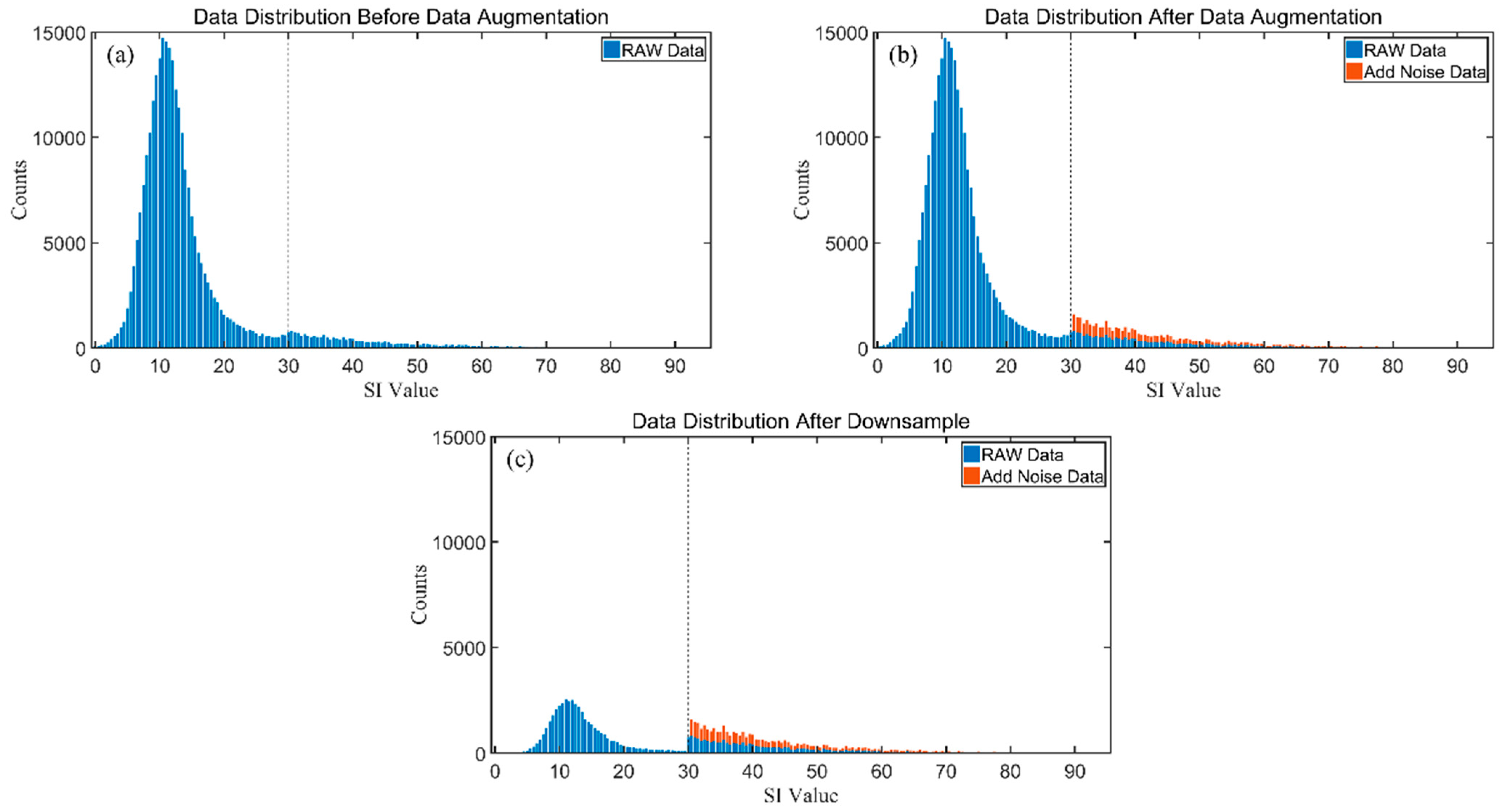
3.1.2. Data Augmentation and Downsampling

As a data-driven algorithmic model, the “long-tailed” phenomenon of the training dataset (i.e., where a few classes have many samples but the remaining majority classes possess much smaller sample sizes) in the machine learning model can lead to poor classification performance for a few classes with limited samples [25], which in turn affects the overall performance of the model. Among the 271,410 training samples used in the experiment, those with SI > 30 are treated as precipitation samples, and those with SI < 30 K are treated as nonprecipitation samples. In this way, the number of precipitation samples is 26,913 (approximately 10%), and the number of nonprecipitation samples is 244,497 (approximately 90%), which is a typical “long-tailed” case. The data distribution is shown in Figure 6a. To solve the “long-tailed” issue, one can scale the sample probabilities such that the sample probability of each class drawn is at the same level as that in [26,27]. Data augmentation techniques can also be used by adding minor changes to the available data (e.g., translation, rotation, clipping, scaling, and noise addition) to create new datasets with larger sizes [28].

In this work, white noise is added to the dataset to augment the precipitation data, as shown in (14).

$$x_{new}=x+\mathit{\mu }+\mathit{\sigma }\times Gaussian\_number$$

(14)

where x represents the original data, x_new represents the new sample obtained after performing data augmentation, μ = 0 and σ = 0.01 represent the mean and variance in the Gaussian function, respectively, and Gaussian_number is a random number that is automatically generated in MATLAB (2017a) and obeys the Gaussian distribution. The data augmentation process expands the original 26,913 precipitation samples to 53,826, the number of precipitation samples increases by 100%, and the total number of samples increases from 271,410 to 298,323. The data augmentation results are shown in the red samples in Figure 6b, and the SIs of all the enhanced samples are greater than 30 K.

To achieve dataset equilibrium, after the precipitation samples are augmented, the nonprecipitation samples are randomly downsampled to make them consistent with the number of precipitation samples (Figure 6c). Then, 80% of the data are randomly selected as the training set, and 20% are selected as the testing set. The results of the data preprocessing strategy are shown in

Table 2. Training and test sets generated using unbalanced data.

	Raw Data	Data Enhancement	Downsampling	Training Set	Testing Set
Nonprecipitation samples	244,497	244,497	53,826	43,060	10,765
Precipitation samples	26,913	53,826	53,826	43,060	10,765

.

3.2. Model Training

After completing preprocessing, the dataset is utilized to train and evaluate the random forest model. The root mean square error (RMSE), mean absolute error (MAE), and coefficient of determination (R2) metrics of the trained model are subsequently evaluated. The definitions of these metrics can be found in (15)–(17), where m represents the number of test samples, RF_SI denotes the simulated scatter index, and SI represents the true scatter index and denotes the average scatter index within the samples.

$$RMSE=\sqrt{{\displaystyle \frac{1}{m}}{{\displaystyle \sum _{i=1}^m(RF\_S{I}_i-S{I}_i)}}^2}$$

(15)

$$MAE={\displaystyle \frac{1}{m}}{\displaystyle \sum _{i=1}^m\left|RF\_S{I}_i-S{I}_i\right|}$$

(16)

$$R2={\displaystyle \frac{{\displaystyle \sum _{i=1}^m{(S{I}_i-RF\_S{I}_i)}^2}}{{\displaystyle \sum _{i=1}^m{(S{I}_i-\overline{SI})}^2}}}$$

(17)

The experimental results are depicted in Figure 7. The RMSE of RF_SI relative to the SI is 1.55 K, the MAE is 0.86 K, and the R2 value is 0.94, indicating strong consistency between RF_SI and the SI overall. In areas with intense scattering (where the SI exceeds 50 K), the average RF_SI is found to be 5 K lower than that of the SI. This discrepancy may be attributed to the complexity of the nonlinear relationship that is inherent in the intense scattering process, which the random forest model may not fully capture. Nonetheless, in the case of strong scattering, RF_SI still demonstrates the ability to accurately identify instances of precipitation, with values exceeding 30 K being indicative of such events. This suggests that RF_SI is well suited for precipitation detection.

3.2.1. Hyperparameters

Hyperparameters are model parameters that need to be set before the training process begins, and they significantly impact the accuracy of the developed model [29].

In this work, we predefine the range of possible values for each hyperparameter and then utilize the “grid search” method [30] to exhaustively explore various combinations of these parameters. Once the program traverses all the parameter combinations, the optimal set is identified and output. In the present study, the utilized hyperparameters are as follows: n_estimators = 120, max_features = 13, min_samples_leaf = 1, and min_samples_split = 3.

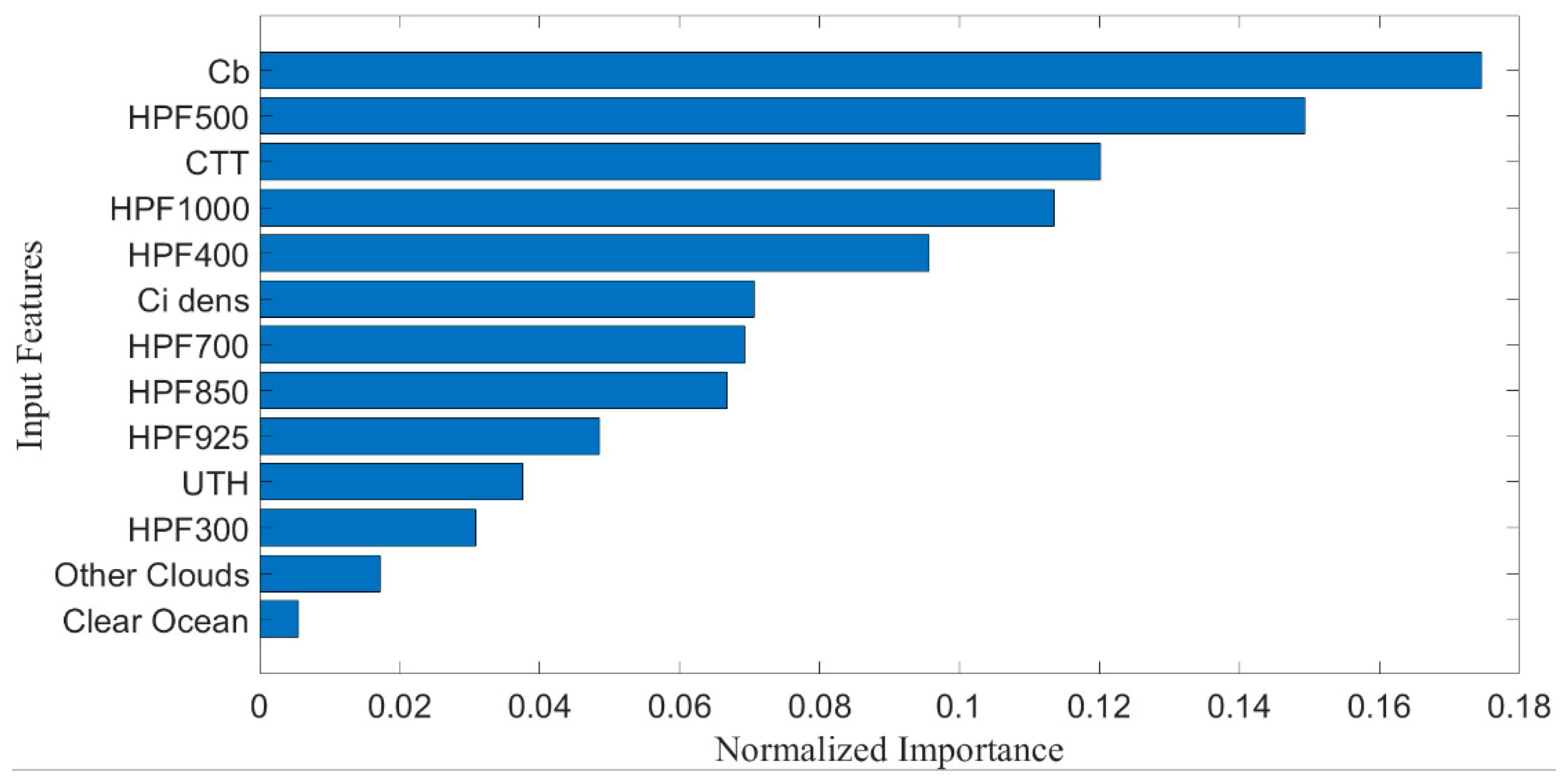
3.2.2. Sensitivity Analysis of the Cloud Parameters

This paper employs the Gini index, which is inherently provided by the scikit-learn version 1.2 software package, to assess the importance of various input variables to the RF_SI model. The relationship between the Gini index and the variable importance levels is as follows. In the context of a random forest, the importance of each input variable is determined by the decrease in the Gini index that results from splitting on that variable. The more a variable reduces the Gini index when used to split a node, the more important it is considered to be for the model.

The sensitivity analysis results obtained for the VISSR inversion products are shown in Figure 8. The figure shows that RF_SI is sensitive to all the input parameters, with the sensitivity values varying from 0.17 to 0.005. Notably, cumulonimbus clouds with strong vertical velocities induce hydrometer sizes that are large enough to trigger microwave scattering at 50–60 GHz. Therefore, RF_SI is most sensitive to cumulonimbus cloud cover data, with a value of 0.17. The cloud region humidity values at 500 hPa and 1000 hPa reflect the condensable water vapor content in the vertical atmospheric column. In particular, the humidity at the 500 hPa level represents the water vapor content that can sustain the phase change exhibited by water under a satisfactory vertical velocity and temperature within the clouds. However, the humidity at 1000 hPa represents the total water vapor content that can be elevated and condensed to multiphase hydrometeors in the upper part of the clouds. The sensitivities of RF_SI to these indicators are 0.15 and 0.11, respectively. Similar mechanisms apply to the humidity values observed for the 400 hPa and 700 hPa cloud regions. The humidity values of the cloud region at 850 hPa and 925 hPa exhibit mechanisms that are analogous to those presented at 1000 hPa. At approximately 300 hPa, the altitude in the divergence zone of clouds and water vapor already undergoes phase changes, and the cloud region humidity indicator is minor, with a value of only approximately 0.03.

The CTT correlates well with the height of the cloud top; when the height is high and the humidity is sufficient, the chance of scattering increases, and clouds can be classified as singular convective clouds or thick cumulus clouds, resulting in a sensitivity of 0.12 for the CTT. Cirrus clouds (Ci) also have a high degree of sensitivity to RF_SI (0.07) because they are good indicators of strong convective cloud anvils and strong convections. However, the “other clouds” class refers to all occurrences of clouds as long as the necessary condition stating that “precipitation occurs in cloud-covered areas” is satisfied. The sensitivity of RF_SI for this scenario is 0.017. Additionally, precipitation is predominantly influenced by convection, and most convection occurs in the lower troposphere. Thus, the sensitivity of the UTH is relatively low (0.04). The “clear ocean” feature has a minimal impact on precipitation, with the lowest importance value of 0.005.

In conclusion, when evaluating the sensitivity of the input features to the microwave spectrum scattering exhibited by hydrometeor particles, the sensitivity rankings obtained from the data-driven machine learning algorithm are highly consistent with those derived from conventional meteorological processes.

4. Results

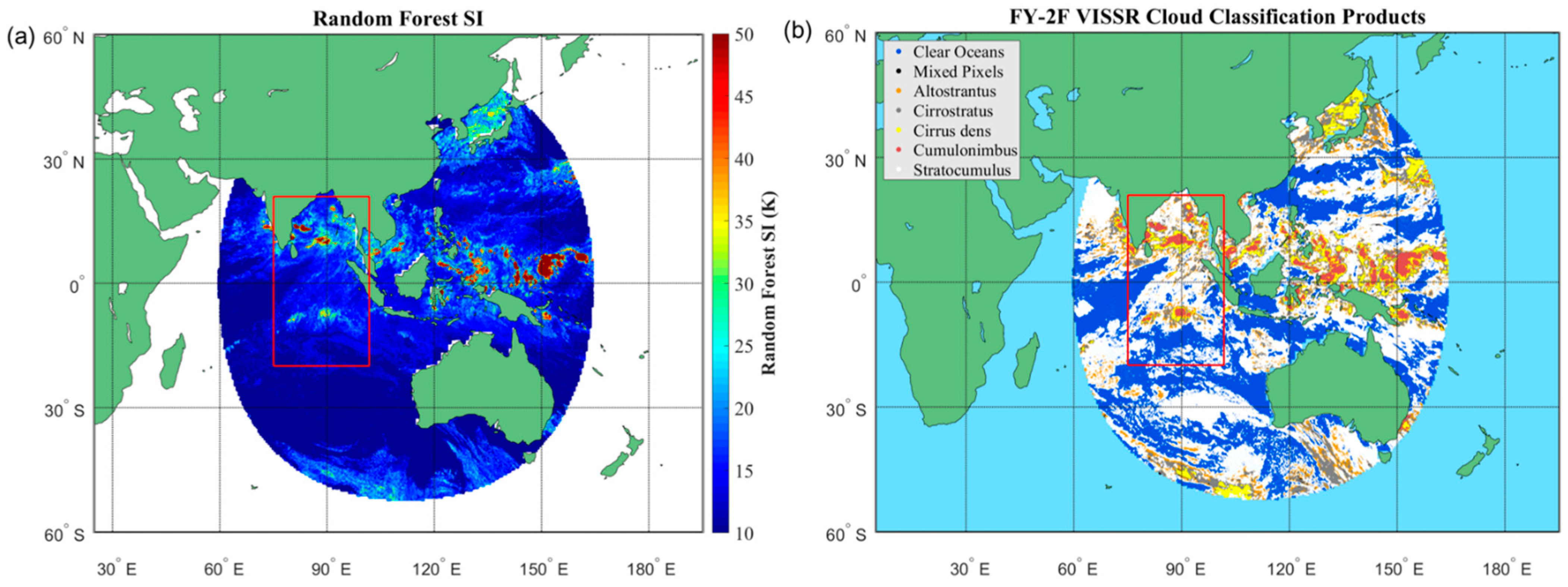
4.1. A Single-Case Analysis

4.1.1. Matching RF_SI to AMSU-A Pixels

Figure 9a shows the RF_SI results produced for the FY-2F pixels obtained via multispectral precipitation detection. Figure 9b shows the FY-2F VISSR pixel-by-pixel CLC product on 6 June 2017, at 21:00 UTC. The red box corresponds to the scanning region of NOAA-19 AMSU-A during transit, with a 7 min observation time difference relative to that of the FY-2F satellite. Figure 9a contains regions with RF_SI values exceeding 45 K along the equator between 120°E and 160°E and in the region between 80°E and 90°E and 5°N and 15°N, which usually corresponds to the cumulonimbus clouds shown in Figure 9b. Near the region at approximately 80°E, 10°S, the RF_SI values, which range between 30 K and 40 K, also correspond to cumulonimbus clouds. However, a large area of cirrus clouds is contained in the Sea of Japan region near the edge of the image, where the average RF_SI is 35 K, which is significantly different from the assumption of convective scattering in the SI description. According to the results of the sensitivity analysis (Figure 8), cirrus information can affect the RF_SI values, and the large number of cirrus clouds contained in the Sea of Japan region with many ice crystal particles may have a complicating effect on microwave scattering, which leads to the calculation of higher RF_SI values. The RF_SI values obtained at approximately 30 K and 35 K in the red box correspond to mixed clouds (equatorial region), but in the region of 30°S, a large area of mixed clouds is present (Figure 9b), corresponding to an average RF_SI of 15 K in Figure 9a, with some differences between the two.

Overall, in the matched spatial and temporal regions, RF_SI has a good correlation with VISSR convective systems, such as cumulonimbus clouds. However, complex microwave scattering caused by large cirrus clouds may bias the RF_SI values. Additionally, may be misclassifications may be observed over the edge areas of VISSR observations.

Figure 10a–c show the pixel analysis results obtained within the scanning region of AMSU-A (corresponding to the red box in Figure 9). The original resolution of the RF_SI products can reach 5 km, whereas the traditional SI and CLWP products have resolutions of only 45 km. To compare RF_SI with the SI at the same resolution, it is necessary to map the high-resolution RF_SI data onto the pixels of AMSU-A, as shown in Figure 10a. Figure 10b displays the AMSU-A SI data, and Figure 10c shows the AMSU-A CLWP data. In the microwave observation images, high SI values (Figure 10b) are present in the regions of the Bay of Bengal (17°N, 92°E and 10°N, 90°E) and the Indian Ocean (10°S, 90°E), with a maximum SI value of 50 K. The corresponding CLWP in Figure 10c also exhibits good correspondence, with a maximum CLWP of 0.9 g/kg, which aligns with the location of the highest SI value. The RF_SI values in the three strong scattering areas also correspond well with the SIs. The RF_SI values produced over the maximum SI value regions are 50 K, demonstrating a largely good degree of location overlap. Additionally, for the weak scattering conditions near 8°S, 82°E, with SI values falling between 30 K and 35 K, the SI and CLWP > 0.5 g/kg correspond well in terms of location. The RF_SI values over these regions are approximately 30 K, so they are largely within the range of the scattering threshold. In the area containing the Gulf of Thailand (13°N, 102°E), which is on the edge of the orbit of AMSU-A, the SI has a value of 25 K, indicating the presence of clouds but without any scattering. The CLWP is identified as a partially cloudy area with 0 g/kg–0.3 g/kg. The RF_SI value is approximately 25 K, and its distribution matches that of the SI. At 13°N, 85°E, where the SI is 24 K and the CLWP is 0.25 g/kg, the area is identified as a cloudy region with no scattering. At this point, RF_SI equals 50, indicating a strong scattering region. Compared with that in Figure 9a, this region corresponds to cumulonimbus clouds in the VISSR image. Although cumulonimbus clouds are the primary contributors to RF_SI, VISSR-based cumulonimbus cloud identification cannot be used to determine their life stages. When the density of cloud hydrometeors is small enough such that they do not induce microwave scattering, both the SI and CLWP demonstrate low values, whereas RF_SI, which is related primarily to the structures of cumulonimbus clouds, remains high. This is one of the limitations found when optical observations are used to retrieve microwave measurement data within clouds.

A further analysis is conducted on the distribution of the AMSU-A pixels contained in the Bay of Bengal region. In Figure 11, pink pixels represent occurrences of precipitation, whereas yellow pixels represent nonprecipitation instances. The grayscale background in the figure represents the VISSR cloud-top brightness temperatures. Figure 11a displays the results produced after the high-resolution RF_SI data are mapped onto the AMSU-A pixels. Notably, good correspondence is observed between the precipitation pixels derived from RF_SI and the regions with low observed brightness temperatures. Figure 11b,c depict the distributions of the AMSU-A SI and CLWP values. The relationships between the SI, CLWP, and brightness temperature are consistent with those shown in Figure 11a. Similar to the SI and CLWP, RF_SI corresponds only to regions with deep convective clouds, effectively indicating the horizontal distribution of microwave scattering. To more clearly demonstrate the effectiveness of the RF_SI precipitation detection approach, the results of the VISSR cloud classification product are visualized in Figure 11d. Upon examination, it can be observed that within the 8–12°N region, RF_SI is capable of detecting a greater number of convective cloud pixels than the SI and CLWP methods can, which highlights the superior performance of RF_SI.

To quantitatively evaluate the RF_SI method via (11)–(13), the ACC, POD, and FAR relative to results of the SI and CLWP methods can be calculated, as shown in

Table 3. ACC, POD, and FAR results produced by the RF_SI method relative to those of the traditional SI and CLWP methods.

	ACC	POD	FAR
RF_SI/SI	96.77%	92.67%	2.02%
RF_SI/CLWP	95.89%	95.70%	6.13%

. The table shows that the ACC of RF_SI relative to the SI is greater than 95%, and the POD and FAR relative to the SI are lower, at 92% and 3%, respectively. In this case, the RF_SI algorithm is comparable to traditional precipitation detection methods that are commonly used.

4.1.2. Matching RF_SI to MWTS2 and MWTS3 Pixels

MWTS2 lacks window channels at 23, 31, and 89 GHz, which precludes the computation of the SI or CLWP. Consequently, quantitatively assessing the precipitation detection performance of RF_SI within MWTS2 is challenging. Therefore, this paper compares the cloud classification results derived from the VISSR CLC for MWTS2.

Figure 12 presents the precipitation detection results obtained with MWTS2 for Typhoon Sula on 31 August 2023 at 05:00 UTC. Specifically, Figure 12a displays the coincidental VISSR CLC product, which delineates the distribution of the cloud bodies at that moment. Figure 12b shows the precipitation detection results produced when the RF_SI method is applied to MWTS2. The RF_SI precipitation detection scheme proposed in this study more accurately discerns the MWTS2 pixels within cumulonimbus regions as precipitation pixels, whereas other areas, including clear skies and nonprecipitation cloud regions, are categorized as nonprecipitation pixels. The future sections on data assimilation applications will assess the efficacy of the RF_SI precipitation detection method in MWTS2 from the perspectives of assimilation and forecasting.

MWTS-III only has observation channels at 23 and 31 GHz but lacks an 89 GHz observation channel, thus preventing the calculation of the SI for MWTS-III. To quantitatively assess the precipitation detection capabilities of the RF_SI method, this study employs the CLWP detection outcomes as the ‘ground truths’. As demonstrated by Weng et al. [5], the CLWP algorithm exhibits a RMSE of 0.05 mm when validated against ground-based microwave radiometer measurements. This study aligns the RF_SI product with MWTS3 pixels and, by evaluating the precipitation detection performance of RF_SI relative to that of the CLWP method, indirectly verifies the applicability of the RF_SI precipitation method to MWTS2. For the precipitation test case, this study selects an extremely intense typhoon, Typhoon Sora, that occurred on 1 September 2023 at 20:00 UTC, and the results are depicted in Figure 13. Figure 13a presents the VISSR cloud classification product, which reveals a substantial amount of deep convective clouds within the typhoon system, and these clouds are typically associated with heavy precipitation. Figure 13b shows the precipitation detection results obtained via the FY-3E MWTS3 CLWP method, where pink denotes precipitation pixels, yellow signifies nonprecipitation pixels, and the background color represents the brightness temperature of the cloud top. Figure 13c displays the precipitation detection results produced after the RF_SI data are matched with the MWTS3 data.

Overall, both the CLWP and RF_SI methods demonstrate the ability to identify typhoon precipitation regions, particularly within the latitudinal range of 13° to 15°N. In this zone, both methods accurately detect nonprecipitation pixels within the convective cloud system, providing clear-sky brightness temperature data between cloud systems. A comparison between Figure 13a and Figure 13b reveals that the CLWP method has a lower degree of sensitivity to convective clouds. In the latitudinal ranges of 11° to 12°N and 20° to 24°N, certain areas covered by convective clouds are not identified as precipitation by the CLWP method. This may be because, despite being covered by convective clouds, the scattering signals derived from the hydrometeors within these areas do not exceed the CLWP threshold. In contrast, the RF_SI method is highly sensitive to convective clouds, often classifying most areas with convective cloud coverage as precipitation. This heightened sensitivity is attributed to the incorporation of the VISSR cloud product as an input feature during the machine learning training process of the RF_SI method. The sensitivity analysis results indicate that convective clouds are most importance to the RF_SI method. To quantitatively assess the precipitation detection capabilities of the RF_SI method, this study employs the CLWP detection outcomes as the ‘ground truths’. Consequently, the ACC of the RF_SI method is calculated to be 0.94, the POD is 0.95, and the FAR is 0.04.

In summary, compared with the CLWP method for MWTS3, the RF_SI method demonstrates better performance in terms of detecting precipitation from convective typhoon cloud systems, and it may be suitable for applications involving precipitation detection endeavors for MWTS2. Furthermore, the RF_SI method is capable of excluding more data from convective cloud areas than the CLWP method is, and the impact of these data on the resulting assimilation and forecasting outcomes warrants further investigation in future studies.

4.2. A Time-Series Analysis

From 6 June 2017 to 6 July 2017, two-per-day FY-2F observations are matched with NOAA-19 transit data within a designated time window. The constructed multispectral precipitation detection algorithm is used to calculate RF_SI, and its results are compared with the SI detection results obtained for paired AMSU-A observations.

4.2.1. Accuracy (ACC), Probability of Detection (POD), and False-Alarm Rate (FAR) Analysis

The VISSR loses information in the VIS band at night, and the accuracy of the RF_SI algorithm needs to be considered separately for both daytime and nighttime scenarios.

The evaluation results shown in Figure 14 indicate that the average ACC and POD of the RF_SI algorithm exceed 94% and 92%, respectively, and the FAR is below 3%.

The mean nighttime ACC and POD are slightly better than those observed during the day, with increases of less than 0.15%, and the nighttime FAR is also slightly lower at 0.03%. These figures demonstrate that the precision of RF_SI is stable and that its variability is low over time. The consistency in performance across different lighting conditions can be attributed to the comprehensive input data (HPF, CTT, CLC and UTH data) required for calculating RF_SI, which include not only VIS/IR information but also background fields, sounding data, and other relevant information. This multifaceted approach ensures that the accuracy of RF_SI is not compromised by variations in day and night conditions. Furthermore, the comparison between RF_SI and the CLWP yields similar results to those of the comparison between the SI and CLWP, which will not be reiterated here (the same analysis follows in the subsequent experiments).

The distribution of paired samples in Figure 5 covers the region between 45°S and 45°N. During this period, the satellite zenith angle range of the FY-2F VISSR is 23.90°–56.13°, and the satellite azimuth angle range for detecting pixels is 94.87°–288.26°. To study the applicability of the RF_SI method over ocean surfaces at midlatitudes, the changes exhibited by the ACC, POD, and FAR of RF_SI under different latitudes are shown in Figure 15a. The paired samples between 10°S and 40°S are distributed mainly across open ocean areas, totaling 7581 samples (shown in Figure 15b). The ACC, POD, and FAR of the RF_SI algorithm are maintained at approximately 95%, 92%, and 3.0%, respectively, with little variation. The number of paired samples between 10°S and 28°N is 20,537, with the ACC and POD of the RF_SI algorithm remaining stable at 95% and 92%, respectively, while the FAR varies between 3.7% and 5.5%. At this time, the paired samples are distributed mainly between Indonesia and the Philippines, where a substantial increase in the FAR of the RF_SI algorithm is observed due to the influence of land. However, the ACC and POD of the RF_SI algorithm, which has a minimal influence on land, maintain similar levels of accuracy to those in the open ocean. Between 28°N and 40°N, the paired sample count decreases significantly to 2495 compared with that in other regions because a substantial portion of the samples are located over East Asia and the South Asia mainland, leading to inadequate representations for analysis purposes.

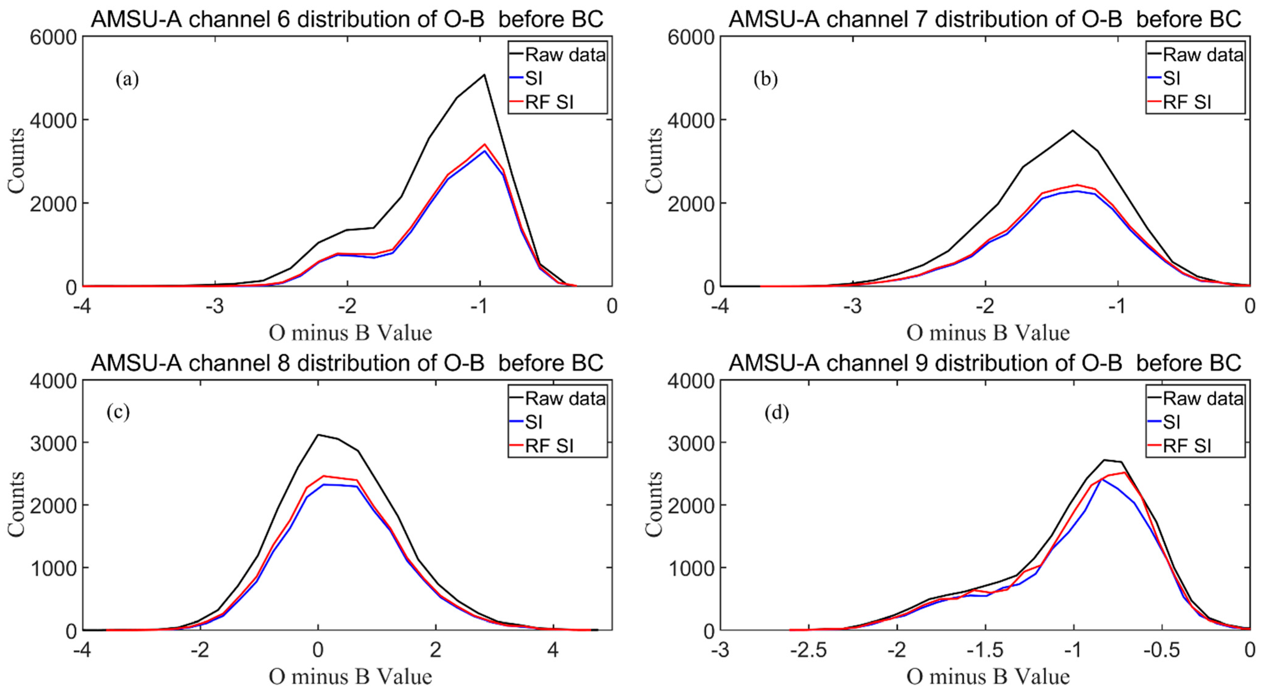
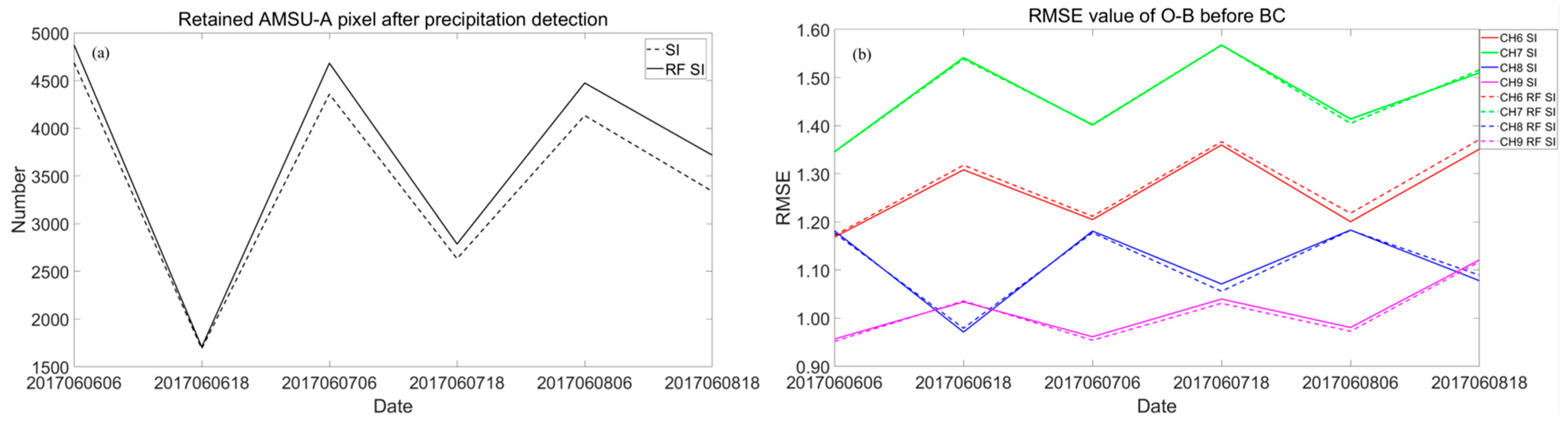
4.2.2. Analysis of the Deviation Between the Observed and Simulated Brightness Temperatures (O-B)

Owing to the scattering effect of precipitation particles, the microwave channel brightness temperatures over precipitation areas are significantly lower than those over clear-sky regions. This subsequently leads to an amplification of the O-B of forward-modeled satellite radiation obtained via clear-sky profiles of temperature and moisture. Precipitation detection relies on high-quality satellite microwave observations that are not contaminated by precipitation, where the O-B before precipitation detection is noticeably lower than the O-B after precipitation detection. The precipitation detection results of RF_SI are expected to have an O-B distribution similar to that of the SI results. The peak weighting function values of channels 6 to 9 of AMSU-A occur between 400 and 90 hPa, and they are influenced considerably by the precipitation occurring within the troposphere. This study focuses on analyzing the O-B distributions of these four channels.

Figure 16 presents the O-B distributions observed before performing bias correction on the nonprecipitation pixels in these four channels. Both the RF_SI and SI methods are capable of filtering out approximately 10–20% of the precipitation pixels from the raw data. Moreover, after the precipitation exclusion step is complete, the O-B distribution trends of the RF_SI and SI methods are consistent, with their curves overlapping relatively well. Channels 6 and 7 exhibit nonrainfall pixels in the ranges of [−3 K, −4.3 K] and [−3.2 K, −3.7 K], respectively. This result suggests that RF_SI might have potential issues when detecting warm cloud precipitation below cirrus clouds. The detection heights of channels 6 and 7 of AMSU-A are below 270 hPa, where large-diameter precipitation particles covered by cirrus clouds are still able to trigger microwave scattering. After performing RF_SI detection, channels 8 and 9 still show samples in both the peak-value and valley-value regions. This finding implies that issues related to the underdetection and overdetection of precipitation are present. Specifically, issues are encountered with respect to performing RF_SI detection via microwave observations under multilayer cloud conditions. In the multilayer cloud cover case, the VISSR can obtain cloud-top information, which may lead to the underidentification or overidentification of precipitation by RF_SI. However, in the peak-value region, RF_SI retains more samples than the SI does.

In the middle and lower levels of the atmosphere, the values detected via the two methods corresponding to the peak data count are basically the same. Compared with those of the SI method, the peak data count values in the upper troposphere (channel 9) are offset by approximately 0.2 K according to the RF_SI method.

For the paired samples collected between 6 June 2017 and 10 June 2017, the daily variation exhibited by the numbers of retained nonprecipitation pixels determined using both detection methods is shown in Figure 17a. The daily statistics reveal that RF_SI retains more nonprecipitation pixels than the SI threshold method does, with a maximum of approximately 500 pixels. Over the five-day period, the SI threshold method retains 20,639 nonprecipitation pixels, whereas RF_SI retains a total of 22,040 pixels, approximately 5% more than the former. Figure 17b displays the RMSE distributions of the O-B results produced for the four channels. The daily RMSE curves of the nonprecipitation pixel O-B distributions obtained after performing RF_SI and SI detection are nearly identical. The O-B RMSEs introduced by both precipitation detection methods are 1.266 K and 1.276 K for channel 6; 1.463 K and 1.462 K for channel 7; 1.111 K and 1.110 K for channel 8; and 1.016 K and 1.011 K for channel 9, respectively, with negligible differences of approximately 10⁻³ K.

5. Discussion

The RF_SI method employs multispectral data as inputs to simulate the nonlinear relationships between infrared and visible light data and microwave precipitation scattering. This method offers a new approach for studying the complicated nonlinear problem concerning microwave precipitation scattering. However, its performance exhibits measurable limitations under complex meteorological regimes (e.g., cirrus clouds, multilayer clouds). To address these constraints, future iterations could integrate alternative machine learning methods (e.g., deep learning, CNNs, U-Net) to enhance sub-pixel feature extraction. Due to the lack of window channels in the MWTS2 instrument, the current validation of RF_SI relies on AMSU-A and MWTS3 as alternative test platforms, representing a notable methodological limitation. The future research will focus on integrating RF_SI into WRFDA data assimilation systems to rigorously assess its practical utility. By quantifying improvements in FY-3C/D MWTS2's data assimilation accuracy and numerical weather prediction skill, this approach will enable direct evaluation of RF_SI’s operational performance while addressing the instrument’s inherent technical constraints. Notably, the algorithm demonstrates marked cross-platform compatibility, with prototype implementations successfully deployed across FY-2F/G/H VISSR and FY-4A/B AGRI sensors, thereby establishing foundational infrastructure for satellite constellation-based precipitation monitoring networks.

6. Conclusions

To solve the precipitation detection problem for FY-3C/D MWTS2, this paper simulates the nonlinear relationships between VISSR cloud products and AMSU-A SIs based on the random forest algorithm. By using GEO-LEO satellite pixel fusion technology, along with the introduction of data preprocessing techniques and model hyperparameter adjustments, this study proposes a novel ocean-surface precipitation detection approach called RF_SI by using four data products derived from the FY-2F VISSR (cloud classification, cloud-top temperature, humidity profile, and water vapor content of the upper troposphere) as input features and NOAA-19 AMSU-A SI values as the learning labels. The precipitation detection performance of the RF_SI method is evaluated through single-case and long-term series observations, which leads us to the following conclusions.

(1)

Data augmentation and downsampling techniques are employed to transform the given imbalanced dataset into a balanced dataset, thereby ensuring a high degree of model fit. An evaluation of the machine learning algorithm reveals that the ranking of the sensitivities of the input features to the particle scattering of microwave spectrum hydrometeors is highly consistent with the existing meteorological knowledge.

(2)

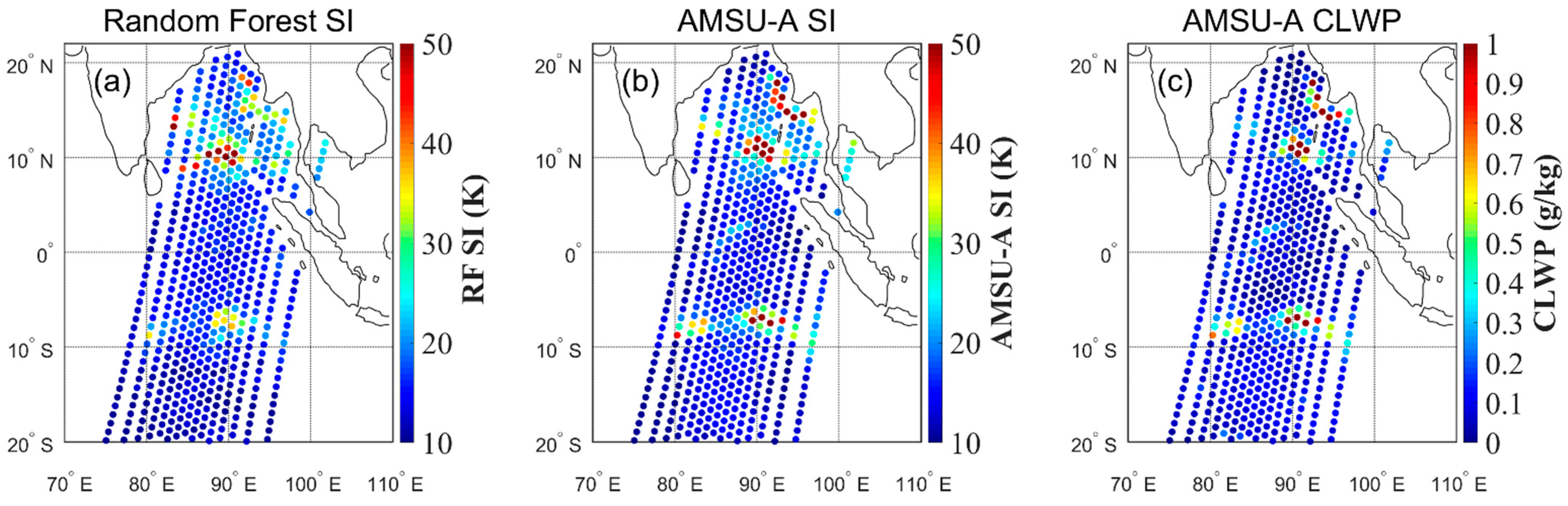
Similar to the SI and CLWP, RF_SI is associated with deep convective cloud regions and therefore is a good indicator of the horizontal distribution of microwave scattering.

(3)

In the time series analysis, the precision of RF_SI is stable, with little change observed over time. Compared with those of the NOAA-19 AMSU-A-based traditional SI and CLWP precipitation detection algorithms, the accuracy and detection rates of the RF_SI method exceed 94% and 92%, respectively, and the error rate is less than 3%.

In future work, high-resolution RF_SI precipitation data obtained through simulations can be matched with FY-3C/3D MWTS2 pixels to address the rapid precipitation detection problem encountered in the WRFDA data assimilation system.

References

1. Geer, A.J.; Baordo, F.; Bormann, N.; Chambon, P.; English, S.J.; Kazumori, M.; Lawrence, H.; Lean, P.; Lonitz, K.; Lupu, C. The growing impact of satellite observations sensitive to humidity, cloud and precipitation. Q. J. R. Meteorol. Soc. 2017, 143, 3189–3206. [Google Scholar] [CrossRef]
2. Bauer, P.; Moreau, E.; Chevallier, F.; O’keeffe, U. Multiple-scattering microwave radiative transfer for data assimilation applications. Q. J. R. Meteorol. Soc. 2006, 132, 1259–1281. [Google Scholar] [CrossRef]
3. Ferraro, R.R.; Weng, F.; Grody, N.C.; Zhao, L. Precipitation characteristics over land from the NOAA-15 AMSU Sensor. Geophys. Res. Lett. 2000, 27, 2669–2672. [Google Scholar] [CrossRef]
4. Yang, Y.; Wei, H.; Peiming, D. Overview on the quality control in assimilation of AMSU microwave sounding data. Meteorol. Mon. 2011, 37, 1395–1401. [Google Scholar]
5. Weng, F.; Zhao, L.; Ferraro, R.R.; Poe, G.; Li, X.; Grody, N.C. Advanced microwave sounding unit cloud and precipitation algorithms. Radio Sci. 2003, 38, 8068. [Google Scholar] [CrossRef]
6. Chen, W.; Chi, J.; Li, Y.; Li, H. Microwave temperature sounding (MWTS) for FY-3 meteorology satellite. Eng. Sci. 2013, 15, 88–91. [Google Scholar]
7. Yang, J.; Zhang, P.; Lu, N.; Yang, Z.; Shi, J.; Dong, C. Improvements on global meteorological observations from the current Fengyun 3 satellites and beyond. Int. J. Digit. Earth 2012, 5, 251–265. [Google Scholar] [CrossRef]
8. Li, J.; Zou, X. A quality control procedure for FY-3A MWTS measurements with emphasis on cloud detection using VIRR cloud fraction. J. Atmos. Ocean. Technol. 2013, 30, 1704–1715. [Google Scholar] [CrossRef]
9. Sun, L.; Fu, Y. A new merged dataset for analyzing clouds, precipitation and atmospheric parameters based on ERA5 reanalysis data and the measurements of TRMM PR and VIRS. Zenodo 2021, 1–26. [Google Scholar] [CrossRef]
10. Qin, L.; Chen, Y.; Ma, G.; Weng, F.; Meng, D.; Zhang, P. Assimilation of FY-3D MWTS-II radiance with 3D precipitation detection and the impacts on typhoon forecasts. Adv. Atmos. Sci. 2022, 40, 900–919. [Google Scholar] [CrossRef]
11. Zhang, J.; Fan, H.; He, D.; Chen, J. Integrating precipitation zoning with random forest regression for the spatial downscaling of satellite-based precipitation: A case study of the Lancang–Mekong River basin. Int. J. Climatol. 2019, 39, 3947–3961. [Google Scholar] [CrossRef]
12. Wang, G.; Ye, S.; Yuan, S.; Jiang, Y. Precipitation estimation by infrared brightness temperature measurement of FengYun-4A imager. In Proceedings of the First International Conference on Spatial Atmospheric Marine Environmental Optics (SAME 2023), Shanghai, China, 7–9 April 2023; pp. 197–200. [Google Scholar]
13. Chen, C.; Hu, B.; Li, Y. Easy-to-use spatial random-forest-based downscaling-calibration method for producing precipitation data with high resolution and high accuracy. Hydrol. Earth Syst. Sci. 2021, 25, 5667–5682. [Google Scholar] [CrossRef]
14. Nguyen, G.V.; Le, X.-H.; Van, L.N.; May, D.T.T.; Jung, S.; Lee, G. Machine learning approaches for reconstructing gridded precipitation based on multiple source products. J. Hydrol. Reg. Stud. 2023, 48, 101475. [Google Scholar] [CrossRef]
15. Kühnlein, M.; Appelhans, T.; Thies, B.; Nauss, T. Improving the accuracy of rainfall rates from optical satellite sensors with machine learning—A random forests-based approach applied to MSG SEVIRI. Remote Sens. Environ. 2014, 141, 129–143. [Google Scholar] [CrossRef]
16. English, S.J.; Renshaw, R.J.; Dibben, P.C.; Smith, A.J.; Rayer, P.J.; Poulsen, C.; Saunders, F.W.; Eyre, J.R. A comparison of the impact of TOVS arid ATOVS satellite sounding data on the accuracy of numerical weather forecasts. Q. J. R. Meteorol. Soc. 2000, 126, 2911–2931. [Google Scholar] [CrossRef]
17. English, S.J.; Renshaw, R.J.; Dibben, P.C.; Eyre, J.R. The AAPP module for identifying precipitation, ice cloud, liquid water and surface type on the AMSU-A grid. In Proceedings of the Ninth International TOVS Study Conference, Igls, Austria, 20–26 February 1997; Eyre, J.R., Ed.; ECMWF: Reading, UK, 1997; pp. 119–130. [Google Scholar]
18. Xu, N.; Hu, X.; Chen, L.; Min, M. Inter-calibration of infrared channels of FY-2/VISSR using high-spectral resolution sensors IASI and AIRS. Natl. Remote Sens. Bull. 2012, 16, 939–952. [Google Scholar] [CrossRef]
19. Breiman, L. Random forests. Mach. Learn. 2001, 45, 5–32. [Google Scholar] [CrossRef]
20. Zhang, Q.; Yu, Y.; Zhang, W.; Luo, T.; Wang, X. Cloud detection from FY-4A’s geostationary interferometric infrared sounder using machine learning approaches. Remote Sens. 2019, 11, 3035. [Google Scholar] [CrossRef]
21. Breiman, L. Bagging predictors. Mach. Learn. 1996, 24, 123–140. [Google Scholar] [CrossRef]
22. Ho, T.K. The random subspace method for constructing decision forests. IEEE Trans. Pattern Anal. Mach. Intell. 1998, 20, 832–844. [Google Scholar] [CrossRef]
23. Breiman, L. Classification and Regression Trees; Routledge: Boca Raton, FL, USA, 2017. [Google Scholar]
24. Han, H.; Lee, S.; Im, J.; Kim, M.; Lee, M.-I.; Ahn, M.H.; Chung, S.-R. Detection of convective initiation using Meteorological Imager onboard Communication, Ocean, and Meteorological Satellite based on machine learning approaches. Remote Sens. 2015, 7, 9184–9204. [Google Scholar] [CrossRef]
25. Zhang, Y.; Kang, B.; Hooi, B.; Yan, S.; Feng, J. Deep long-tailed learning: A survey. arXiv 2021, arXiv:2110.04596. [Google Scholar] [CrossRef] [PubMed]
26. Kang, B.; Xie, S.; Rohrbach, M.; Yan, Z.; Gordo, A.; Feng, J.; Kalantidis, Y. Decoupling representation and classifier for long-tailed recognition. arXiv 2019, arXiv:1910.09217. [Google Scholar]
27. Wang, T.; Li, Y.; Kang, B.; Li, J.; Liew, J.H.; Tang, S.; Hoi, S.C.H.; Feng, J. The devil is in classification: A simple framework for long-tail instance segmentation. In Proceedings of the Computer Vision—ECCV 2020, Glasgow, UK, 23–28 August 2020; pp. 728–744. [Google Scholar]
28. Li, B.; Hou, Y.; Che, W. Data augmentation approaches in natural language processing: A survey. AI Open 2021, 3, 71–90. [Google Scholar] [CrossRef]
29. Wang, B.; Gong, N.Z. Stealing hyperparameters in machine learning. In Proceedings of the 2018 IEEE Symposium on Security and Privacy (SP), San Francisco, CA, USA, 20–24 May 2018; pp. 36–52. [Google Scholar]
30. Sun, Y.; Wang, Y.; Guo, L.; Ma, Z.; Jin, S. The comparison of optimizing SVM by GA and grid search. In Proceedings of the 2017 13th IEEE International Conference on Electronic Measurement & Instruments (ICEMI), Yangzhou, China, 20–22 October 2017; pp. 354–360. [Google Scholar]
Figure 1. The methodological diagram of the RF_SI precipitation.
Remotesensing 17 01566 g001
Figure 2. Distribution of the FY-2F VISSR cloud retrieval product at 00:00 on 1 January 2018. (af) Relative humidity values at various levels from 300–1000 hPa; (g) cloud classification products; (h) cloud-top temperature; and (i) relative humidity values in the middle and upper levels of the troposphere.
Remotesensing 17 01566 g002
Figure 3. Example of the matching process performed for VISSR pixels that satisfy the dmax threshold within a given AMSU-A pixel.
Remotesensing 17 01566 g003
Figure 4. Schematic diagram of the multispectral precipitation identification method based on the random forest algorithm. (a) Decision tree and (b) random forest.
Remotesensing 17 01566 g004
Figure 5. FY-2F and NOAA-19 observations that satisfied the pairing conditions (a) at 06:00 UTC during the day and (b) at 21:00 UTC during the night on 2 January 2018. Red markers indicate observations satisfying the matching criteria, and yellow markers denote observations that do not meet the matching conditions.
Remotesensing 17 01566 g005
Figure 6. Distribution of the training dataset, including (a) raw data; (b) augmented data, and (c) data acquired after performing downsampling. Red represents the new data obtained after adding Gaussian white noise.
Remotesensing 17 01566 g006
Figure 7. Scatter plot of the SI and RF_SI values in the testing dataset.
Remotesensing 17 01566 g007
Figure 8. Gini importance of the VISSR retrieval products within the training dataset. Cb represents cumulonimbus clouds, HPF300-HPF1000 represents the relative humidity at 300–1000 hPa, CTT represents the cloud-top temperature, Ci dens represents dense cirrus clouds, UTH represents the relative humidity in the middle and upper levels of troposphere, “Other Clouds” represents other types of clouds, and “Clear Ocean” represents a clear-sky surface.
Remotesensing 17 01566 g008
Figure 9. Comparison between FY-2F-retrieved cloud parameters and those of RF_SI at 21:00 UTC on 6 June 2017. (a) RF_SI values derived from random forest model simulations (the red box corresponds to the scanning region of NOAA-19 AMSU-A during transit) and (b) FY-2F VISSR cloud classification products.
Remotesensing 17 01566 g009
Figure 10. Pixel analysis of the AMSU-A scanning region: (a) RF_SI results, (b) AMSU-A SI, and (c) AMSU-A CLWP.
Remotesensing 17 01566 g010
Figure 11. Precipitation detection results obtained for the Bay of Bengal region in terms of different indicators by (a) RF_SI; (b) the SI; (c) and CLWP (the pink points represent occurrences of precipitation, and the yellow points represent nonoccurrences of precipitation). (d) The FY-2F VISSR CLC products.
Remotesensing 17 01566 g011
Figure 12. Precipitation detection results obtained with FY-3D MWTS2 for Typhoon Sula on 31 August 2023 at 05:00 UTC: (a) VISSR cloud classification products and (b) the precipitation detection results yielded by MWTS2/RF_SI.
Remotesensing 17 01566 g012
Figure 13. Precipitation detection results obtained with FY-3D MWTS3 for Typhoon Sula on 1 September 2023 at 20:00 UTC: (a) VISSR cloud classification products; (b) the precipitation detection results of CLWP; and (c) the precipitation detection results of RF_SI.
Remotesensing 17 01566 g013
Figure 14. Time series analysis of RF_SI from 6 June 2017 to 6 July 2017. (a) ACC; (b) POD; and (c) FAR.
Remotesensing 17 01566 g014
Figure 15. Latitude analysis of RF_SI. (a) Variations in the ACC, POD, and FAR values of RF_SI and (b) the distribution of data along the latitudinal gradient.
Remotesensing 17 01566 g015
Figure 16. The statistical O-B results obtained for channels 6–9: (ad) after removing the AMSU-A precipitation pixels via the SI and RF_SI methods at 18:00 UTC on 6 June 2017 (before performing bias correction).
Remotesensing 17 01566 g016
Figure 17. Time series of (a) the retained pixel numbers and (b) RMSEs of O-B for channels 6–9 after performing AMSU-A precipitation detection via the SI and RF_SI methods from 06:00 UTC on June 6 to 18:00 UTC on 8 June 2017.
Remotesensing 17 01566 g017