Exploring the Effectiveness of Fusing Synchronous/Asynchronous Airborne Hyperspectral and LiDAR Data for Plant Species Classification in Semi-Arid Mining Areas

Abstract

Plant species classification in semi-arid mining areas is of great significance in assessing the environmental impacts and ecological restoration effects of coal mining. However, in semi-arid mining areas characterized by mixed arbor–shrub–herb vegetation, the complex vegetation distribution patterns and spectral features render single-sensor approaches inadequate for achieving fine classification of plant species in such environments. How to effectively fuse hyperspectral images (HSI) data with light detection and ranging (LiDAR) to achieve better accuracy in classifying vegetation in semi-arid mining areas is worth exploring. There is a lack of precise evaluation regarding how these two data collection approaches impact the accuracy of fine-scale plant species classification in semi-arid mining environments. This study established two experimental scenarios involving the synchronous and asynchronous acquisition of HSI and LiDAR data. The results demonstrate that integrating LiDAR data, whether synchronously or asynchronously acquired, significantly enhances classification accuracy compared to using HSI data alone. The overall classification accuracy for target vegetation increased from 71.7% to 84.7% (synchronous) and 80.2% (asynchronous), respectively. In addition, the synchronous acquisition mode achieved a 4.5% higher overall accuracy than asynchronous acquisition, with particularly pronounced improvements observed in classifying vegetation with smaller canopies (Medicago sativa L.: 17.4%, Pinus sylvestris var. mongholica Litv.: 11.7%, and Artemisia ordosica Krasch.: 7.5%). This study can provide important references for ensuring classification accuracy and error analysis of land cover based on HSI-LiDAR fusion in similar scenarios.

1. Introduction

At this stage, China′s coal mines are mainly located in semi-arid areas, where water resources are in short supply, and mining activities change the surface morphology and intensify the runoff and evaporation processes, directly affecting the growth of vegetation and the stability of ecosystems [1]. High-intensity mining activities cause continuous disturbance to the surrounding ecological environment, resulting in covert ecological degradation of the mining environment [2,3]. Plants are important and comprehensive dominant indicators of ecological disturbance in semi-arid mining areas. The accurate classification of plants can help to identify the damaged vegetation areas and ecosystem succession stages, which is of great significance for assessing the environmental transfer effects caused by coal mining and evaluating the ecological restoration effects in China [4,5].

Satellite remote sensing technology has the ability of large-scale coverage, can obtain the vegetation information of large mining areas in a relatively short period of time, and is suitable for long-term and large-scale ecological monitoring and assessment, but the data resolution is limited and the classification error is large [6]. In recent years, unmanned aerial vehicles (UAVs) have achieved great success in many application scenarios including vegetation classification in semi-arid areas, and this success is mainly attributed to the flexibility of their mounted sensors and the high resolution of their data [7,8]. Airborne multispectral sensors are able to capture information about the differences in plant responses in different bands, which can help to distinguish between different species and their health status [9]. Jeong et al. [10] developed a support vector machine model based on multispectral data that was able to effectively classify cabbage, rice, and soybean, in which the recursive feature elimination (RFE) model achieved an overall accuracy (OA) of 88.64% with a Kappa coefficient of 0.84. Mao et al. [11] captured images during the flowering period of maize by an airborne Sequoia multispectral sensor, which accurately reflected the changes in chlorophyll content, providing technical support for field crop growth monitoring and accurate fertilization decisions. However, the number of bands in multispectral remote sensing is small, which makes it difficult to distinguish vegetation species with similar spectral characteristics. HSI which has richer spectral data in bands, shows great potential in semi-arid areas, and can distinguish the differences in reflectance characteristics of plants in different narrow bands, improving the accuracy of species identification [12]. Zhan et al. [13] used HSI combined with a support vector machine algorithm to classify the vegetation in the target area, and distinguished the vegetation types such as pine forest, broadleaf forest, and shrub based on spectral features, which could still maintain high robustness in the case of insufficient samples. Liang et al. [14] proposed a spectral-spatial parallel convolutional neural network to classify the forest species based on the HSI imagery of UAVs and achieved 97.91% OA. In recent years, the synergistic application of HSI and machine learning algorithms has shown significant technical advantages and great application potential in the field of feature classification [15,16,17]. However, HSI data cannot acquire ground-object vertical distribution information [18]. More and more studies have shown that the fusion of LiDAR data, which can acquire spatial three-dimensional information on ground objects, with HSI data with complementary advantages can achieve better classification accuracy [19,20,21,22]. Daeyeol Kim et al. [23] conducted a study on urban-scale tree classification. They extracted the vegetation spectral index using HSI. This approach effectively characterizes the spectral response of chlorophyll, carotenoids, and other biochemical components. Additionally, they used LiDAR to extract the maximum tree height, leaf area index, and symmetry difference index of the canopy structure. These metrics were used to quantitatively characterize the heterogeneity of the canopy structure and seasonal volume change. Li et al. [24] addressed the issue of the uneven distribution of taxonomic demands caused by different wetland mangrove areas. They used HSI data to select key areas, such as the red edge and near-infrared bands, to characterize the spectral feature differences of different plant leaves. Meanwhile, LiDAR data utilized multidimensional features, such as the canopy height model, vertical quartile, and structural heterogeneity, to describe the vertical structure and spatial heterogeneity distribution of vegetation communities. The LiDAR data employed multidimensional features, like the canopy height model, vertical quartile, and structural heterogeneity, to characterize the vertical structure and spatial heterogeneity of vegetation communities. The selection of HSI and LiDAR fusion classification features varies greatly for the fine classification needs of features in different regions. For the semi-arid mining areas in China, where trees, shrubs, and grasses are mixed and the heterogeneity of spatial distribution is high, how to better integrate the HSI and LiDAR data to realize the fine classification of plants is an issue worth studying.

Airborne HSI and LiDAR are mostly located along track sensors, and the reliable geo-localization of the acquired data presupposes known accurate position and attitude information during flight [25]. The position and attitude information of the sensors is usually obtained through data post-processing of a tightly combined GNSS/INS navigation system [26,27,28]. Existing airborne HSI and LiDAR data acquisition can be categorized into two modes, i.e., synchronous and asynchronous acquisition [29]. Hyperspectral and LiDAR synchronous acquisition refers to the rigid integration of both sensors on a single UAV. During each UAV mission, hyperspectral and LiDAR data are simultaneously collected while sharing identical position and attitude datasets. Asynchronous acquisition involves a separate mounting of hyperspectral and LiDAR sensors on UAV platforms, requiring two distinct UAV missions to independently collect hyperspectral and LiDAR data, each accompanied by independent position and attitude datasets. Due to the continuous high-frequency vibration of the UAV acquisition platform and frequent large-attitude braking during the actual data acquisition process, there are dynamic model perturbation errors, observation coarseness, and random sensor errors during the sensor position data solving process. These factors lead to large differences in the position solving results between multiple flights [30,31]. Wu et al. [32] showed that the UAV will be affected by the aerodynamic force generated by the rotating paddles and its own mass during the flight process, which leads to nonlinear changes in the position parameters of the UAV, and then generates cumulative errors in the navigation solving system. Feng et al. [33] showed that the vibration noise of the paddle disk during the flight process of the co-axial UAV will interfere with the accelerometers and gyroscopes, and is prone to drift and spin during the flight process, which leads to errors in data acquisition. In the process of flight, it is easy for offset, spin, and other phenomena to appear and lead to data acquisition error. Theoretically, the data discrepancy of the position sensors will directly lead to the inability to strictly align homonymous features between the HSI and LiDAR data acquired by multiple sorties. At the same time, when collecting vegetation information, the HSI and LiDAR data acquired by multiple sorties will also introduce multiple environmental errors. These errors are caused by changes in meteorological factors during the radiometric correction process. This will affect the accuracy of the fusion application of HSI and LiDAR [34].

Therefore, in this study, we designed two sets of experiments to acquire HSI and LiDAR data synchronously and asynchronously. These experiments were conducted using an airborne HSI and LiDAR integrated monitoring system that shares a combined GNSS/INS navigation module. We also carried out a fusion test of airborne HSI and LiDAR data for the classification of plant species in semi-arid mining areas. The goal was to quantitatively evaluate the impact of fusing synchronous and asynchronous airborne HSI and LiDAR data on the fine classification of plant species in these areas. The impact of fusing synchronized and asynchronous airborne HSI and LiDAR data on the fine classification of plant species in semi-arid mining areas was quantitatively evaluated. This paper can provide a scientific basis for the subsequent application of the fusion of airborne HSI and LiDAR data in the classification of plant species in semi-arid mining areas, which has certain theoretical and practical significance.

2. Materials and Methods

2.1. Overview of the Study Area and Data Acquisition

The study area is located in the artificial restoration area of the Daliuta Mining Area Soil and Water Conservation Park in Yulin City Shaanxi Province, with a regional average annual temperature of about 6.2 °C and annual precipitation of about 300–400 mm. Precipitation is mainly concentrated in the summer, and evapotranspiration exceeds rainfall by more than four times, which is typical for an arid and semi-arid plateau continental climate [35]. Located in the transition zone between steppe and forest grassland, the main vegetation types are trees, scrub, sandy type vegetation, and steppe, and the main plant varieties are Populus simonii Carr., Pinus sylvestris var, mongholica Litv., Cerasus pseudocerasus Lindl., Armeniaca sibirica (Linn.) Lam., Cerasus humilis (Bunge) Bar. and Liou, Salix psammophila C. Wang et Ch. Y. Yang, Hippophae rhamnoides Linn., Caragana korshinskii Kom., Amorpha fruticosa Linn., Artemisia ordosica Krasch., Medicago sativa L., and other herbaceous plants (Figure 1). The average elevation of the area is about 1200 m. The average altitude of the area is around 1200 m, with large topographic ups and downs.

The combined HSI imager, LiDAR, and inertial guidance receiver was physically integrated into the UAV to ensure synchronized data acquisition, see Figure 2. The first synchronized acquisition of five HSI imagery and LiDAR point clouds of the study area was made at an altitude of 100 m at a speed of 10 m/s relying on the UAV-carried integrated ground monitoring system, and the second separate acquisition of five LiDAR point clouds of the study area was made in August 2021.

This study focuses on the fine species classification of trees represented by Populus simonii Carr., Pinus sylvestris var. mongholica Litv., Cerasus pseudocerasus Lindl., Armeniaca sibirica (Linn.) Lam., and Cerasus humilis (Bunge) Bar. and Liou, shrubs represented by Salix psammophila C. Wang et Ch. Y. Yang., Hippophae rhamnoides Linn., Caragana korshinskii Kom., Amorpha fruticosa Linn., and Artemisia ordosica Krasch., and herbaceous plants consisting of Medicago sativa L. and other herbaceous plants. To enable the training and testing of the classification model, a number of sampling points were randomly recorded throughout the study area using the GPS RTK positioning mode by species at the same time as the HSI and LiDAR data collection. Of these, there were 236 Populus simonii Carr., 366 Pinus sylvestris var. mongholica Litv., 87 Cerasus pseudocerasus Lindl., 99 Armeniaca sibirica (Linn.) Lam., 322 Cerasus humilis (Bunge) Bar. and Liou, 128 Salix psammophila C. Wang et Ch. Y. Yang, 301 Hippophae rhamnoides Linn., 505 Caragana korshinskii Kom., 247 Amorpha fruticosa Linn., 401 Artemisia ordosica Krasch., 88 Medicago sativa L., and 428 other herbaceous plants.

The spectra at the sampling points of the 12 plant types were averaged and their average spectral curves were calculated as shown in Figure 3. It can be seen from the figure that the 12 plant types have similar spectral curves, especially in the visible band, implying that it is difficult to achieve fine classification using only spectral information.

2.2. Plant Multi-Attribute Features Extraction

2.2.1. HSI Features

(1)

Spectral Transformation Features

HSI remote sensing images have high spectral resolution and many bands, but there is a certain correlation between the bands, and there is a large amount of redundant information, and processing all of the band ranges is not only time-consuming, but also too many linear bands may affect the final classification accuracy. Therefore, multiband HSI data should be processed by dimensionality reduction to extract the most effective spectral information. Principal component analysis was performed on the HSI images, and the first three principal components (PCA1, PCA2, and PCA3) of the transformed HSI images were selected as the spectral transformed features and participated in the subsequent texture feature extraction and classification studies.

(2)

Texture Features

Texture features reflect the spatial structure of the plant canopy and are an important factor in distinguishing plant species. The gray-level co-occurrence matrix (GLCM) is the most commonly used texture feature extraction method, which describes the texture by counting the spatial correlation properties of grayscale on the target image, and derives the texture information matrix by calculating the grayscale relationship of neighboring pixels or pixels within a certain distance [36]. The GLCM provides comprehensive information about the direction, adjacency interval, and magnitude of change in the gray level of an image.

To more intuitively describe the texture condition through the symbiotic matrix, mean, variance, homogeneity, contrast, dissimilarity, information entropy, second moment, and correlation are derived from the symbiotic matrix. The correlation is calculated for eight parameters that reflect the condition of the matrix. In this chapter, based on the spectral transform features (PCA1, PCA2, and PCA3), the eight texture parameters of the three components are extracted, and a total of 24 texture features are obtained, and their calculation formulas and descriptions are shown in

Table 1. Texture feature parameters corresponding to three principal components.

Texture Features	Abbreviation	Calculation Formula	Description
Mean	PCA1_M; PCA2_M; PCA3_M	${\displaystyle {\displaystyle \sum }_i}{\displaystyle {\displaystyle \sum }_j}i·P\left(i,j\right)$	Indicates the average degree of grayscale in the image
Variance	PCA1_V; PCA2_V; PCA3_V	${\displaystyle {\displaystyle \sum }_i}{\displaystyle {\displaystyle \sum }_j}{(i-\mu )}^{2}P\left(i,j\right)$	Indicates the degree of grayscale change in the image
Homogeneity	PCA1_H; PCA2_H; PCA3_H	${\displaystyle {\displaystyle \sum }_i}{\displaystyle {\displaystyle \sum }_j}P\left(i,j\right)/[1+\left(i-j{)}^2\right]$	Represents local homogeneity in the image
Contrast	PCA1_Ct; PCA2_Ct; PCA3_Ct	${\displaystyle {\displaystyle \sum }_i}{\displaystyle {\displaystyle \sum }_j}P\left(i,j\right){(i-j)}^2$	Indicates the sharpness of the image and the depth of the grooves in the texture
Differences	PCA1_D; PCA2_D; PCA3_D	${\displaystyle {\displaystyle \sum }_i}{\displaystyle {\displaystyle \sum }_j}\left|i-j\right|P\left(i,j\right)$	Represents a localized area texture feature in an image
Information entropy	PCA1_E; PCA2_E; PCA3_E	$-{\displaystyle {\displaystyle \sum }_i}{\displaystyle {\displaystyle \sum }_j}P\left(i,j\right)\log P\left(i,j\right)$	A measure of randomness that represents the amount of information contained in an image
Second-order moment	PCA1_S; PCA2_S; PCA3_S	${\displaystyle {\displaystyle \sum }_i}{\displaystyle {\displaystyle \sum }_j}P{(i,j)}^2$	Represents the uniformity of the grayscale distribution of the image and the thickness of the texture
Correlation	PCA1_CoPCA2_Co; PCA3_Co	${\displaystyle {\displaystyle \sum }_i}{\displaystyle {\displaystyle \sum }_j}\left(i-{\mu }_x\right)\left(j-{\mu }_y\right)P\left(i,j\right)/{\sigma }_x{\sigma }_y$	Indicates how similar the image is at the gray level

Note: $P\left(i,j\right)$ represents $P\left(g_1,g_2\right)$, where ${\mu }_x$, ${\mu }_y$, ${\sigma }_x$, and ${\sigma }_y$ represent the row and column means and standard deviations, respectively.

.

(3)

Vegetation Indices

Vegetation indices are usually obtained by multi-band calculation, and at this stage, scholars have proposed many vegetation indices for various target needs, and most of them can enhance a certain physiological and ecological feature or detail of plants, and a reasonable selection of vegetation indices can effectively improve the accuracy of fine classification results. Considering the semi-arid climate characteristics of the study area, ten relevant indices that can reflect the vegetation canopy structure, chlorophyll content, and water and stress were selected in this paper, and their calculation formulas and descriptions are shown in

Table 2. Vegetation indexs for classification.

Abbreviation	Description	Calculation Formula	Bibliography
B30	Reflectance at 550 nm (green peak)		Haboudane et al. [37]
B67	Reflectance at 750 nm (NIR shoulder)		Haboudane et al. [37]
C1	Chlorophyll Index 1	$\mathrm{C}1=({\rho }_{850}-{\rho }_{710})/({\rho }_{850}+{\rho }_{680})$	Datt [38]
C2	Chlorophyll Index 2	$\mathrm{C}2={\rho }_{750}/{\rho }_{700}$	Datt [38]
PSI	Plant Stress Index	$\mathrm{P}\mathrm{S}\mathrm{I}={ \rho }_{695}/{\rho }_{760}$	Carter and Miller [39]
NDVI	Normalized Difference Vegetation Index	$\mathrm{N}\mathrm{D}\mathrm{V}\mathrm{I}=({\rho }_{800}-{\rho }_{670})/({\rho }_{800}+{ \rho }_{670})$	Rouse et al. [40]
PRI	Photochemical Reflectance Index	$\mathrm{P}\mathrm{R}\mathrm{I}=({\rho }_{531}-{\rho }_{570})/({\rho }_{531}+{\rho }_{570})$	Gamon et al. [41]
RVSI	Red-edge Vegetation Stress Index	$\mathrm{R}\mathrm{V}\mathrm{S}\mathrm{I}=({\rho }_{714}-{\rho }_{752})/2-{\rho }_{733}$	Merton [42]
PSSR	Pigment Specific Simple Ratio	$\mathrm{P}\mathrm{S}\mathrm{S}\mathrm{R}={\rho }_{800}/{\rho }_{635}$	Blackburn [43]
WBI	Water Band Index	$\mathrm{W}\mathrm{B}\mathrm{I}={\rho }_{970}/{\rho }_{900}$	Penuelas et al. [44]

.

2.2.2. LiDAR Features

(1)

Intensity Information

LiDAR intensity reflects, to a certain extent, the reflectivity of the target scanned by LiDAR pulses, which varies in energy with the composition of the surface object reflecting the echo [45]. Specifically, for the application of vegetation classification, the morphology and proportions of branches, trunks, and leaves of different plant types vary; in other words, the energy of the reflected echoes from different plant types theoretically varies, and thus plant species can be recognized based on the LiDAR intensity. In this study, the point cloud was geo-corrected and intensity-corrected, and then rasterized and interpolated to 0.2 m to obtain the whole intensity information of the study area, which is denoted by INT.

(2)

Canopy Height

The canopy height model (CHM) is the most used vegetation structure parameter extracted by LiDAR and has been proven to be an important contribution to plant species classification in a large number of studies. The accuracy of CHM extraction will directly determine the final classification results of plants, especially for species with highly similar spectral curves and differences in canopy height. In this paper, the LiDAR last echo point cloud is used as the data source, and the method proposed by Tian et al. [46] is used to obtain the canopy height model (CHM).

2.3. Plant Fine Classification Method Based on Multi-Feature Fusion

2.3.1. Random Forest and Multi-Scale Segmentation Fusion Classification

Multidimensional features may be highly correlated or redundant with each other, and too many feature variables not only increase the computational complexity, but also easily lead to dimensionality catastrophe, i.e., the Hughes phenomenon, which results in a decrease in prediction or classification accuracy [47]. Therefore, sample feature variables usually need to be ranked and screened for feature variable importance before practical application, with respect to retaining the features with greater contribution. In this paper, the random forest model is selected as an integrated classifier for feature importance ranking and screening and the preliminary categorization of plant species. HSI features are input along with LiDAR feature elements, and feature variables are ranked and screened based on their importance. Features with greater contribution are retained to achieve a preliminary categorization of plant species at the pixel level.

While random forest can provide basic classification results, the classification results tend to be noisier and more misclassified because pixel-level classification ignores spatial contextual information. The multi-scale segmentation technique uses eCognition 9.0 software to further cluster pixels into objects with semantic information on top of the initial pixel-level classification. Combining the spectral features and spatial contextual information of the pixels makes the classification results more in line with the actual distribution and structural characteristics of the plants, thus reducing the noise and uncertainty in the classification and improving the accuracy of the classification.

2.3.2. Classification Accuracy Evaluation Method

The final classification results need to undergo quantitative accuracy validation. The confusion matrix is one of the most used methods for accuracy validation [48]. The factors derived from it for accurate evaluation include the following:

(1)

Producer Accuracy (PA)

The ratio of the correctly classified number of a certain type of plant $X_{ii}$ in the error matrix to the total number of true reference samples of that species $X_{+i}$, reflecting the probability of a certain type of plant being correctly classified.

(2)

User Accuracy (UA)

The ratio of the correctly classified number of a certain type of plant $X_{ii}$ in the error matrix to the total number of samples classified as that species $X_{i+}$.

$$P_{UA}={\displaystyle \frac{X_{ii}}{X_{i+}}}$$

(3)

Overall Accuracy (OA)

The percentage of the total number of correctly classified species out of the total number of samples $M$, representing the overall correctness of species classification, with the total number of correctly classified pixels of each type of plant located on the diagonal of the matrix.

$$P_{0A}={\displaystyle \frac{{\sum }_{i=1}^{n }{X}_{ii}}{M}}$$

(4)

Kappa Coefficient

An accuracy statistic calculated based on the elements of the error matrix, reflecting the match between the classification results and the actual species categories, and providing a more objective evaluation of the classification accuracy.

$$Kappa={\displaystyle \frac{M{\sum }_{i=1}^n{X}_{ii}-{\sum }_{i=1}^{n }{X}_{i+}{X}_{+i}}{M^2-{\sum }_{i=1}^n{X}_{i+}{X}_{+i}}}$$

3. Results

3.1. Impact of Asynchronous Data Collection on HSI and LiDAR Data Registration Accuracy

Due to the effect of random errors, there are some differences between the accuracy of the two positional solutions (

Table 3. Basic indicators of synchronous/asynchronous data.

Datasets		POS Precision		Relative Offset (cm)	HSI Variability (Trees, Irrigation Book, Herb, and Earth)
		Location (m)	Attitude (°)
Synchronous acquisition	HSI/LiDAR	[0.0235, 0.0292, 0.0411]	[0.0489, 0.0504, 0.1732]	14.1	[1.27, 2.16, 1.76, 1.67]
Asynchronous acquisition	HSI LiDAR	[0.0235, 0.0292, 0.0411] [0.0258, 0.0272, 0.0460]	[0.0489, 0.0504, 0.1732] [0.0423, 0.0457, 0.1654]	32.3	[1.39, 2.44, 1.94, 1.71]

). These errors will be directly introduced into the asynchronously acquired HSI and LiDAR data generation process, resulting in irregular scaling and offset between the HSI image and LiDAR point cloud layers. Even after manual stab point alignment was performed, an offset of 32.3 cm between the asynchronously acquired HSI and LiDAR layers was found using the relative positioning checkpoint statistics, which is much larger than the HSI ground resolution (20 cm). Therefore, the asynchronously acquired HSI and LiDAR data are not strictly aligned, and there is an irregular offset of about 1.5 pixels between them. Since the HSI radiometric correction process needs to rely on the slope and slope direction information provided by the corresponding LiDAR data, the non-strict alignment of the HSI and LiDAR data will have a certain impact on the HSI radiometric correction effect. From the statistical results, the HSI spectral variability under synchronized acquisition shows a small reduction in the spectral variability of the same geographical category compared with asynchronous acquisition.

3.2. Feature Screening and Dimensionality Reduction

In this study, three spectral transform features (PCA1, PCA2, and PCA3), 24 texture features, 10 vegetation indices (B30, B67, C1, C2, PSI, NDVI, PRI, RVSI, PSSR, and WBI), one intensity feature (INT), and one canopy height feature (CHM) were extracted, totaling 39 feature variables. They were combined and superimposed to form a set of categorical feature variables. By repeatedly ranking the importance of the above feature variables, 16 feature combinations were finally identified, including two spectral transformation features (PCA2 and PCA3), three texture features (PCA1_M, PCA2_M, and PCA3_M), nine spectral indices (B30, C1, C2, PSI, NDVI, PRI, RVSI, PSSR, and WBI), one intensity feature (INT), one intensity feature (INT), and one canopy height feature (CHM), totaling 39 feature combinations. One intensity feature (INT), one canopy height feature (CHM), and the importance of each feature variable in the synchronous collection/asynchronous collection group are shown in Figure 4.

As can be seen from the figure, the ordering of the importance of the feature variables in the synchronous acquisition/asynchronous acquisition group is basically the same, with only minor differences in the ordering of individual features. Among the 16 feature variables remaining in the screening, the spectral index occupies the vast majority. Only PCA2 and PCA3 were retained for the spectral variation features, where PCA3 was much more important than PCA2, and PCA1 did not appear in the optimal feature set due to the inclusion of data noise in it and its low contribution to plant classification. Texture features were all eliminated by the importance of filtering algorithms except for the mean feature which indicates the average degree of grayscale of the principal components. Vegetation canopy height derived from the LiDAR point cloud had the most significant effect on species classification accuracy, much higher than other feature variables, while plant intensity features also obtained from LiDAR had a relatively weak effect. Through the comprehensive analysis of the screening results of the feature variables, the canopy height, green band reflectance, the third component of spectral transformation that can reflect the shape and smoothness of the canopy to a certain extent, and the average grayscale value are the main factors for distinguishing the plant species in the semi-arid study area. This conclusion is also basically in line with the actual situation in the field.

3.3. Multi-Scale Segmentation Fusion

The parameters of the multi-scale segmentation algorithm mainly contain three key factors: scale parameter, shape, and spectrum. Among them, the scale parameter can be set independently, the weight of the shape and spectral factors is one, and the shape factor can be subdivided into tightness and smoothness. The parameter settings determine the quality of the segmentation results, and improper selection of parameters can cause problems such as “over-segmentation” and “under-segmentation”. In this paper, several experiments are carried out to explore the optimal parameter combinations adapted to the study area, and some of the results are listed in Figure 5. Specifically, the left column of Figure 5 shows the changes in multi-scale segmentation results when the fixed scale parameter is 90, the tightness weight is 0.5, and the shape weight is changed step by step (0–1, with a step size of 0.1), which demonstrates that the size of the plaques is inversely proportional to the shape weights; the middle column of Figure 5 shows the changes in multi-scale segmentation results when the fixed scale parameter is 40 and the shape weight is 0.1, which demonstrates an inverse proportion to the shape weight. When the shape weight is fixed at 40 and the shape weight is 0.1, the tightness weight is changed step by step (0–1, step size 0.1), the change in multi-scale segmentation results can be seen in that the plaque size is directly proportional to the tightness weight. The right column of Figure 5 is the change in multi-scale segmentation results when the shape weight is fixed at 0.1 and the tightness weight is 0.5; the change in the scale parameter is changed step by step (5, 10, and 20), and the change in the plaque size and the scale parameter can be seen in that the size of the plaque is directly proportional to the scale parameter as well.

By observing the segmentation results and analyzing the subsequent plant species classification requirements, the final combination of scale parameters of five, a shape weight of 0.1, and a tightness weight of 0.5 was selected as the final parameters for this experiment. The above parameters were used to obtain the multi-scale image segmentation results, with each of the vectors as a statistical unit and with the help of the ArcMap raster statistics tool for the preliminary classification map unit voting to export the final classification map.

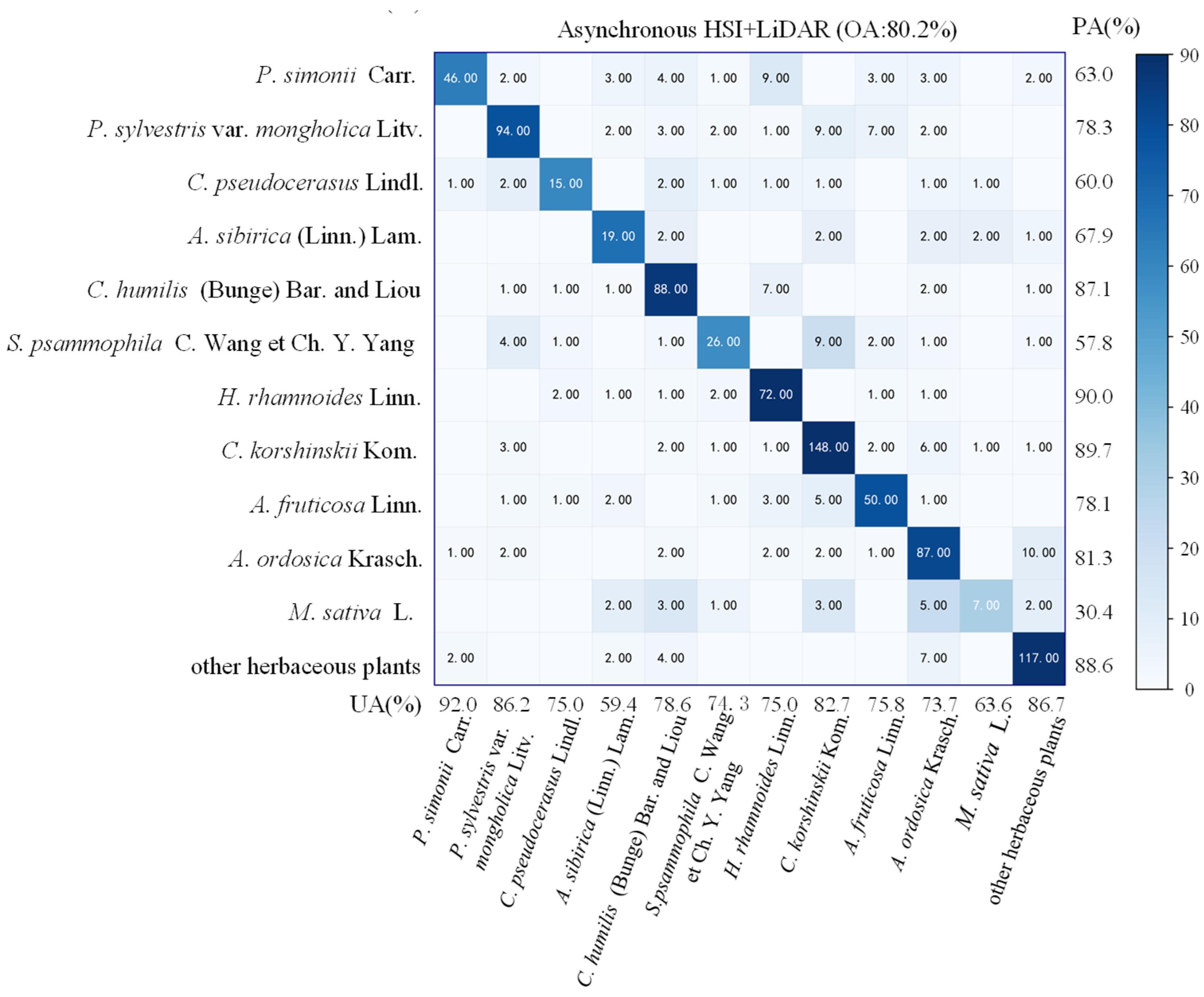
3.4. Comparative Analysis of Plant Species Taxonomic Results

The filtered feature components were classified into three groups: (1) using only HSI-derived features (HSI); (2) a combination of synchronously acquired HSI- and LiDAR-derived features (synchronously acquired HSI+LiDAR); and (3) a combination of asynchronously acquired HSI- and LiDAR-derived features (asynchronously acquired HSI+LiDAR). Using the random forest classifier and combining the results of multi-scale segmentation to classify them, respectively, the final plant classification results of the study area are shown in Figure 6. The differences between the two groups of feature classification results can be clearly seen in the figure, and the synchronous and asynchronous acquisition of the HSI+LiDAR-derived plant species types are more aggregated compared to the HSI results, with Populus simonii Carr., Pinus sylvestris var. mongholica Litv., Hippophae rhamnoides Linn., and Salix psammophila C. Wang et Ch. Y. Yang being the most obvious, which is consistent with the actual situation in the field. This is consistent with the actual situation at the site; this area is an artificial restoration area, and the same type of plant grows in succession due to the planting method, which is common.

Figure 7 presents the confusion matrices for classification using the three datasets, summarizing the producer and user accuracy for the final classification of each plant species in each of the three cases. From the figure, it is observed that the classification accuracies varied greatly among the 12 plant species. The PA using only the HSI dataset ranged from 34.8% (Medicago sativa L.) to 88.5% (Caragana korshinskii Kom.), and the UA ranged from 53.5% (Medicago sativa L.) to 92.9% (Cerasus pseudocerasus Lindl.). The PA using the synchronous acquisition HSI and LiDAR fusion dataset ranged from 47.8% (Medicago sativa L.) to 93.4% (Hippophae rhamnoides Linn.) and the UA ranged from 74.1% (Armeniaca sibirica (Linn.) Lam.) to 100% (Medicago sativa L.). The PA using asynchronously collected HSI and LiDAR fusion datasets ranged from 30.4% (Medicago sativa L.) to 90.0% (Hippophae rhamnoides Linn.), and the UA ranged from 63.6% (Medicago sativa L.) to 92.0% (Populus simonii Carr.). A higher classification accuracy for Hippophae rhamnoides Linn., Caragana korshinskii Kom., and other herbaceous plants was achieved when using only the HSI dataset, and Pinus sylvestris var. mongholica Litv., Cerasus humilis (Bunge) Bar. and Liou, Hippophae rhamnoides Linn., Caragana korshinskii Kom., Amorpha fruticosa Linn., Artemisia ordosica Krasch., and other herbaceous plants can be recognized with a high degree of accuracy.

Table 4. Accuracy statistics for plant classification results obtained by using three variable sets.

Dataset	Tree OA (%)	Shrub OA (%)	Herb OA (%)	12 Species OA (%)	12 Species Kappa
HSI	60.2	78.1	78.7	71.7	0.68
Synchronous HSI + LiDAR	83.0	86.1	84.5	84.7	0.83
Asynchronous HSI + LiDAR	75.5	83.1	80.0	80.2	0.78

compares the quantitative accuracies of plant species classification using the three datasets, and the classification accuracies after the fusion of synchronously collected and asynchronously collected HSI+LiDAR datasets are both greatly improved compared to the use of the HSI dataset only. The OA of the 12 plants increased from 71.7% to 84.7% and 80.2%, and the kappa coefficient increased from 0.68 to 0.83 and 0.78, respectively. The OA of the trees (Populus simonii Carr., Pinus sylvestris var. mongholica Litv., Cerasus pseudocerasus Lindl., Armeniaca sibirica (Linn.) Lam., and Cerasus humilis (Bunge) Bar. and Liou) increased from 60.2% to 83.0% and 75.5%, respectively. Shrubs (Salix psammophila C. Wang et Ch. Y. Yang., Hippophae rhamnoides Linn., Caragana korshinskii Kom., Amorpha fruticosa Linn., and Artemisia ordosica Krasch.) increased from 78.1% to 86.1% and 83.1%, respectively. Herbs (Medicago sativa L. and other herbaceous plants) improved from 78.7% to 84.5% and 80.0%, respectively. The addition of LiDAR features substantially improved the overall classification accuracy of trees and slightly improved the overall classification accuracy of shrubs and grasses, especially the canopy height feature, which effectively avoided the mixing of trees and shrubs. In addition, using the synchronized acquisition of HSI+LiDAR improved OA by 4.5% and the kappa coefficient by 0.05 compared to asynchronously acquired data. Some of the plant types showed a significant increase in PA, such as Medicago sativa L., Pinus sylvestris var. mongholica Litv., and Artemisia ordosica Krasch. by 17.4%, 11.7%, and 7.5%, respectively.

4. Discussion

Clarifying the importance of HSI and LiDAR feature variables is crucial for vegetation classification in semi-arid mining areas [49,50]. In this study, the order of importance of feature variables in the synchronous/asynchronous acquisition group was basically the same, with only minor differences in the order of individual features. Among them, the spectral index features accounted for the majority, proving that the spectral index contains a large amount of information that can be used to differentiate species by category. Among all of the spectral indices, the PRI and B30 features associated with the green band, accounted for a higher importance, while the near-infrared band, which is more capable of recognizing species in other studies, was rather insignificant in the classification of plants in this study area [51,52,53]. The possible reason is that the plant leaf morphology in the study area varies greatly. The sensitivity of the green band to chlorophyll absorption and scattering information is more likely to highlight the differences between vegetation and sparse vegetation, which can better reflect the small changes in the physiological state of vegetation. In contrast, the reflected signals of the near-infrared band are often significantly affected by background interference under sparse canopy conditions. This results in a reduced ability to discriminate between different species. The vegetation in the study area covers a wide range of trees, shrubs, and herbs, and the characteristics of canopy height are particularly important. Canopy height provides structural information in distinguishing different vegetation, which can directly reflect the vertical distribution and growth status of vegetation. The experimental data showed that the fusion of HSI and LiDAR improved the classification accuracy of each vegetation compared with using only HSI data. Among these, the classification accuracy of trees showed the greatest improvement (asynchronous: 15% and synchronous: 23%). Similar to the findings of Picos, J et al. [54], the reason for this is that trees exhibit a distinct vertical structure, and the inclusion of canopy height features can effectively reduce the misclassification of trees as shrubs and herbs. In contrast, the role of plant intensity features acquired by LiDAR was relatively weak, related to the fact that most species in the study area have thinner branches and smaller leaves, and the difference in the reflected intensity of laser light is not obvious.

In this study, the difference in the classification accuracy of vegetation in the study area between the synchronized acquisition of HSI and LiDAR data and asynchronous acquisition of HSI and LiDAR data was quantified. The largest difference in identification accuracy occurred in the case of trees, with a difference of 8%, followed by herbaceous plants at 4.5%, and the smallest difference was in the case of shrubs at 3%. Trees show a discrete spatial distribution pattern in the study area, and their morphological characteristics are characterized by small crown widths and significant heights [55], which are extremely sensitive to the spatial matching accuracy of HSI and LiDAR data. These methods are extremely sensitive to the spatial matching accuracy of HSI and LiDAR data. In asynchronous acquisition, an offset of 32.3 cm occurs between the HSI image and the LiDAR point cloud due to two flight position resolution errors. As a result, the spectral reflectance of the top of the tree canopy may be matched with the canopy height data of neighboring low-growth vegetation. This mismatch leads to the failure of feature fusion, reducing classification accuracy. In some cases, the correspondence between the point cloud and the HSI pixels may be entirely lost, which affects the correlation between the CHM and spectral features. In the study area, shrub vegetation has a simple and uniform structure with continuous spatial distribution. It exhibits low heterogeneity in HSI and LiDAR data, and its growth status and canopy structure changes are small in magnitude [56]. This results in a low difference between the two acquisition modes in terms of data characteristics, making the impact on classification accuracy relatively limited. The accuracy is reduced by only about 3%. Medicago sativa L. had the highest omission rate among the plant species classification results. The main reason is that Medicago sativa L. has a small canopy radius, the average canopy width is less than 0.5 m, and the branches are extremely thin and the leaf area index is very small, which makes it difficult to accurately capture the canopy height and density information in LiDAR data [57,58]. Based on the spatial distribution characteristics of Medicago sativa L. and the structural characteristics of the species, it is extremely sensitive to the spatial matching accuracy of HSI and LiDAR data, and the PA of the asynchronous fusion of the HSI and LiDAR data of Medicago sativa L. was 30.4% in the experimental data, while that of the synchronous fusion of HSI and LiDAR data increased to 47.8% in the experimental data. Based on the spatial distribution characteristics of Medicago sativa L. and the structural characteristics of the species, it is extremely sensitive to the spatial matching accuracy of HSI and LiDAR data. In the experimental data, the PA of the asynchronous fusion of the HSI and LiDAR data of Medicago sativa L. was 30.4%, while the PA of the synchronous fusion of HSI and LiDAR data increased to 47.8%. The important influence of synchronous and asynchronous acquisition on the accuracy of the remote sensing monitoring of Medicago sativa L. was revealed.

In addition, due to the specificity of vegetation growth conditions in the study area, the canopy width of trees was generally low and did not differ much from that of shrubs, which could easily lead to the confusion between trees and shrubs [59]. The other vegetation misclassified as trees was dominated by shrubs, and the difference between the canopy widths of trees and shrubs was insignificant. This was the main reason for the decrease in the UA of trees. The tree structure is usually more stratified, and the local leaf area index values may be higher and show a clear vertical gradient, while the spatial distribution of shrub vegetation is continuous, and its leaf area distribution is more uniform. Utilizing the distribution characteristics of LAI in different height strata can help to capture the differences in the internal structure of the two types of vegetation. The height distribution statistics of the point cloud data, such as selecting 90% and 95% point cloud data, can more accurately reflect the differences in the vertical structure of the plant canopy, and it is expected that the classification accuracy of arboreal, shrubs, and grasses will be further improved through these methods, which is the focus of our next study.

The airborne hyperspectral and LiDAR devices used in this study are two cutting-edge and complementary perceptual sensors. Their integration can not only be applied to plant classification but also holds extensive potential in fields such as precision agriculture and geological and mineral exploration. However, it is regrettable that their substantial costs prevent many researchers from acquiring both sensors simultaneously. This practical limitation reduces the referential value of our research for other scholars. Additionally, it is important to note that while our findings demonstrate the significant impact of fusing synchronously/asynchronously acquired hyperspectral and LiDAR data on plant classification outcomes, the classification accuracy of their fusion applications remains influenced by numerous factors. These include complex data preprocessing workflows and fusion-classification methodologies. Studies indicate that the rigorous geometric correction, radiometric calibration, and point cloud filtering of airborne hyperspectral and LiDAR data can effectively enhance data reliability [60,61]. Moreover, when the plant features extracted from two sensors are sufficiently abundant, fusing them through deep learning methods may achieve higher classification accuracy compared to machine learning. Incorporating the convolutional block attention module (CBAM) into deep learning methods could enhance classifier performance by enabling the model to focus on critical plant classification-related features while suppressing irrelevant noise [62]. Therefore, we recommend that researchers systematically consider potential error sources when working with these costly hyperspectral and LiDAR datasets to ensure the accuracy of their results.

5. Conclusions

HSI/LiDAR asynchronous acquisition fusion classification has advantages over single HSI or LiDAR classification. The spectral curves of the 12 plant types in the study area have high similarity, and it is difficult to realize fine classification by relying only on HSI sensors. LiDAR data can provide accurate vegetation structure information, which effectively compensates for the shortcomings of HSI data. Quantitative statistical results show that the vegetation classification accuracy of the fusion of HSI and LiDAR data is significantly improved compared to using HSI data alone. Synchronized acquisition ensures the temporal and spatial consistency of the HSI and LiDAR data. It also avoids the accumulation of sensor position resolution errors and environmental random errors caused by different flights in asynchronous acquisition. These errors could result in the HSI and LiDAR layers being unable to align strictly, thus affecting subsequent data processing and analysis. Synchronized acquisition ensures a pixel-level alignment of the data and reduces errors due to data mismatch. The classification accuracy of the fused HSI and LiDAR data from synchronized acquisition is higher than that of the asynchronous data, and the OA of the synchronized acquisition is 84.7%, while the OA of the asynchronous acquisition is 80.2%. The results indicate that synchronized acquisition has advantages over asynchronous acquisition in the airborne HSI and LiDAR integrated monitoring system.

This study explores the accuracy difference between synchronous and asynchronous LiDAR and HSI data in the application scenario of plant classification in semi-arid mines. The fusion application of the two has a wide range of applications in the fields of urban planning, agricultural monitoring, environmental protection, and resource investigation. In our future research, we will continue to explore the accuracy difference between fused feature classification using synchronously acquired and asynchronously acquired HSI and LiDAR data. This exploration will focus on different application scenarios, monitoring objects, feature extraction methods (e.g., partial least squares), and fusion methods. We hope that our study can provide valuable theoretical insights and practical frameworks for the scientific community engaged in multimodal remote sensing analysis, particularly for researchers seeking to advance feature classification methodologies through the effective integration of HSI and LiDAR technologies.

References

1. Li, X.; Lei, S.; Cheng, W.; Liu, F.; Wang, W. Spatio-temporal dynamics of vegetation in Jungar Banner of China during 2000–2017. J. Arid Land 2019, 11, 837–854. [Google Scholar] [CrossRef]
2. Wu, Z.; Lei, S.; Lu, Q.; Bian, Z. Impacts of Large-Scale Open-Pit Coal Base on the Landscape Ecological Health of Semi-Arid Grasslands. Remote Sens. 2019, 11, 1820. [Google Scholar] [CrossRef]
3. Li, X.; Lei, S.; Liu, Y.; Chen, H.; Zhao, Y.; Gong, C.; Bian, Z.; Lu, X. Evaluation of Ecological Stability in Semi-Arid Open-Pit Coal Mining Area Based on Structure and Function Coupling during 2002–2017. Remote Sens. 2021, 13, 5040. [Google Scholar] [CrossRef]
4. Li, J.; Zhou, X.; Yan, J.; Li, H.; He, J. Effects of regenerating vegetation on soil enzyme activity and microbial structure in reclaimed soils on a surface coal mine site. Appl. Soil Ecol. 2015, 87, 56–62. [Google Scholar] [CrossRef]
5. Li, S.; Xiao, W.; Zhao, Y.; Lv, X. Incorporating ecological risk index in the multi-process MCRE model to optimize the ecological security pattern in a semi-arid area with intensive coal mining: A case study in northern China. J. Clean. Prod. 2020, 247, 119143. [Google Scholar] [CrossRef]
6. Hai, W.; Xia, N.; Song, J.; Tang, M. Identification and Monitoring of Surface Elements in Open-Pit Coal Mine Area Based on Multi-Source Remote Sensing Images. Pol. J. Environ. Stud. 2022, 31, 4127–4136. [Google Scholar] [CrossRef]
7. Sun, Z.; Wang, X.; Wang, Z.; Yang, L.; Xie, Y.; Huang, Y. UAVs as remote sensing platforms in plant ecology: Review of applications and challenges. J. Plant Ecol. 2021, 14, 1003–1023. [Google Scholar] [CrossRef]
8. Li, L.; Zheng, X.; Zhao, K.; Li, X.; Meng, Z.; Su, C. Potential Evaluation of High Spatial Resolution Multi-Spectral Images Based on Unmanned Aerial Vehicle in Accurate Recognition of Crop Types. J. Indian Soc. Remote Sens. 2020, 48, 1471–1478. [Google Scholar] [CrossRef]
9. Guo, T.; Kujirai, T.; Watanabe, T. Mapping Crop Status from An Unmanned Aerial Vehicle for Precision Agriculture Applications. In Proceedings of the XXII ISPRS Congress, Technical Commission I, Melbourne, Australia, 25 August–1 September 2012; Volume 39-B1, pp. 485–490. [Google Scholar]
10. Jeong, C.-H.; Go, S.-H.; Park, J. Classification of Fall Crops Using Unmanned Aerial Vehicle Based Image and Support Vector Machine Model—Focusing on Idam-ri, Goesan-gun, Chungcheongbuk-do -. J. Korean Soc. Rural. Plan. 2022, 28, 57–69. [Google Scholar]
11. Mao, Z.; Deng, L.; Sun, J.; Zhang, A.; Chen, X.; Zhao, Y. Research on the Application of UAV Multispectral Remote Sensing in the Maize Chlorophyll Prediction. Spectrosc. Spectr. Anal. 2018, 38, 2923–2931. [Google Scholar]
12. Paoletti, M.; Haut, J.; Plaza, J.; Plaza, A. Deep learning classifiers for hyperspectral imaging: A review. ISPRS-J. Photogramm. Remote Sens. 2019, 158, 279–317. [Google Scholar]
13. Zhan, Y.; Hu, D.; Wang, Y.; Yu, X. Semisupervised Hyperspectral Image Classification Based on Generative Adversarial Networks. IEEE Geosci. Remote Sens. Lett. 2018, 15, 212–216. [Google Scholar] [CrossRef]
14. Liang, J.; Li, P.; Zhao, H.; Han, L.; Qu, M. Forest Species Classification of UAV Hyperspectral Image Using Deep Learning. In Proceedings of the 2020 Chinese Automation Congress (CAC 2020), Shanghai, China, 6–8 November 2020; pp. 7126–7130. [Google Scholar]
15. Paoletti, M.; Haut, J.; Fernandez-Beltran, R.; Plaza, J.; Plaza, A.; Li, J.; Pla, F. Capsule Networks for Hyperspectral Image Classification. IEEE Trans. Geosci. Remote Sens. 2019, 57, 2145–2160. [Google Scholar] [CrossRef]
16. Zhu, L.; Chen, Y.; Ghamisi, P.; Benediktsson, J. Generative Adversarial Networks for Hyperspectral Image Classification. IEEE Trans. Geosci. Remote Sens. 2018, 56, 5046–5063. [Google Scholar] [CrossRef]
17. Li, S.; Song, W.; Fang, L.; Chen, Y.; Ghamisi, P.; Benediktsson, J. Deep Learning for Hyperspectral Image Classification: An Overview. IEEE Trans. Geosci. Remote Sens. 2019, 57, 6690–6709. [Google Scholar] [CrossRef]
18. Patro, R.; Subudhi, S.; Biswal, P.; Dell’acqua, F. A Review of Unsupervised Band Selection Techniques: Land Cover Classification for Hyperspectral Earth Observation Data. IEEE Geosci. Remote Sens. Mag. 2021, 9, 72–111. [Google Scholar] [CrossRef]
19. Liu, H.; Bruning, B.; Garnett, T.; Berger, B. Hyperspectral imaging and 3D technologies for plant phenotyping: From satellite to close-range sensing. Comput. Electron. Agric. 2020, 175, 105621. [Google Scholar] [CrossRef]
20. Zhang, Q.; Luan, R.; Wang, M.; Zhang, J.; Yu, F.; Ping, Y.; Qiu, L. Research Progress of Spectral Imaging Techniques in Plant Phenotype Studies. Plants 2024, 13, 3088. [Google Scholar] [CrossRef]
21. Omia, E.; Bae, H.; Park, E.; Kim, M.; Baek, I.; Kabenge, I.; Cho, B. Remote Sensing in Field Crop Monitoring: A Comprehensive Review of Sensor Systems, Data Analyses and Recent Advances. Remote Sens. 2023, 15, 354. [Google Scholar] [CrossRef]
22. Fassnacht, F.; Latifi, H.; Sterenczak, K.; Modzelewska, A.; Lefsky, M.; Waser, L.; Straub, C.; Ghosh, A. Review of studies on tree species classification from remotely sensed data. Remote Sens. Environ. 2016, 186, 64–87. [Google Scholar] [CrossRef]
23. Kim, D.; Song, Y.; Kim, H.; Kwon, O.; Yeon, Y.; Lim, T. Airborne multi-seasonal LiDAR and hyperspectral data integration for individual tree-level classification in urban green spaces at city scale. Int. J. Appl. Earth Obs. Geoinf. 2025, 136, 104319. [Google Scholar] [CrossRef]
24. Li, Q.; Wong, F.K.K.; Fung, T. Mapping multi-layered mangroves from multispectral, hyperspectral, and LiDAR data. Remote Sens. Environ. 2021, 258, 112403. [Google Scholar] [CrossRef]
25. Jiang, W.; Li, Y.; Rizos, C. Improved decentralized multi-sensor navigation system for airborne applications. GPS Solut. 2018, 22, 78. [Google Scholar] [CrossRef]
26. Xu, Y.; Du, B.; Zhang, L.; Cerra, D.; Pato, M.; Carmona, E.; Prasad, S.; Yokoya, N.; Hänsch, R.; Le Saux, B. Advanced Multi-Sensor Optical Remote Sensing for Urban Land Use and Land Cover Classification: Outcome of the 2018 IEEE GRSS Data Fusion Contest. IEEE J. Sel. Top. Appl. Earth Observ. Remote Sens. 2019, 12, 1709–1724. [Google Scholar] [CrossRef]
27. Gao, B.; Hu, G.; Gao, S.; Zhong, Y.; Gu, C. Multi-sensor Optimal Data Fusion for INS/GNSS/CNS Integration Based on Unscented Kalman Filter. Int. J. Control Autom. Syst. 2018, 16, 129–140. [Google Scholar] [CrossRef]
28. Elamin, A.; Abdelaziz, N.; El-Rabbany, A. A GNSS/INS/LiDAR Integration Scheme for UAV-Based Navigation in GNSS-Challenging Environments. Sensors 2022, 22, 9908. [Google Scholar] [CrossRef] [PubMed]
29. Dronova, I.; Taddeo, S. Remote sensing of phenology: Towards the comprehensive indicators of plant community dynamics from species to regional scales. J. Ecol. 2022, 110, 1460–1484. [Google Scholar] [CrossRef]
30. You, D.; Hao, Y.; Xu, J.; Yang, L. Research on Attitude Detection and Flight Experiment of Coaxial Twin-Rotor UAV. Sensors 2022, 22, 9572. [Google Scholar] [CrossRef]
31. Lin, H.; Zhan, J. GNSS-denied UAV indoor navigation with UWB incorporated visual inertial odometry. Measurement 2023, 206, 112256. [Google Scholar] [CrossRef]
32. Wu, Z. Design of Helicopter Rotor Noise Laboratory (Anechoic Chamber). Noise Vib. Control 2020, 40, 207–209. [Google Scholar]
33. Feng, Z.; Hao, Y.; You, D.; Yang, L.; Sun, S.; Zhong, T. Experimental Study on the Effect of Coaxial UAV Rotor Disk Vibration on Attitude Stability. Vib. Shock 2025, 44, 151–159. [Google Scholar]
34. Xu, Y.; Li, J.; Du, C.; Chen, H. NBR-Net: A Nonrigid Bidirectional Registration Network for Multitemporal Remote Sensing Images. IEEE Trans. Geosci. Remote Sens. 2022, 60, 5620715. [Google Scholar] [CrossRef]
35. Liu, Y. Research on Vegetation Restoration Guided by Damaged Vegetation in Semi-arid Coal Mine Areas. Ph.D. Thesis, China University of Mining and Technology, Beijing, China, Web of Science. 2020. Available online: https://link.cnki.net/doi/10.27623/d.cnki.gzkyu.2020.000513 (accessed on 20 April 2025).
36. Haralick, R.M.; Shanmugam, K.; Dinstein, I. Textural Features for Image Classification. IEEE Trans. Syst. Man Cybern. 1973, SMC-3, 610–621. [Google Scholar] [CrossRef]
37. Haboudane, D.; Miller, J.R.; Pattey, E.; Zarco-Tejada, P.J.; Strachan, I.B. Hyperspectral vegetation indices and novel algorithms for predicting green LAI of crop canopies: Modeling and validation in the context of precision agriculture. Remote Sens. Environ. 2004, 90, 337–352. [Google Scholar] [CrossRef]
38. Datt, B. A New Reflectance Index for Remote Sensing of Chlorophyll Content in Higher Plants: Tests using Eucalyptus Leaves. J. Plant Physiol. 1999, 154, 30–36. [Google Scholar] [CrossRef]
39. Carter, G.A.; Miller, R.L. Early detection of plant stress by digital imaging within narrow stress-sensitive wavebands. Remote Sens. Environ. 1994, 50, 295–302. [Google Scholar] [CrossRef]
40. Rouse, J.W.; Haas, R.H.; Schell, J.A.; Deering, D.W. Monitoring Vegetation Systems in the Great Plains with ERTS. Third ERTS-1 Symposium NASA, NASA SP-351; NASA: Washington, DC, USA; pp. 309–317.
41. Gamon, J.A.; Green, R.O.; Roberts, D.A. Deriving photosynthetic function from calibrated imaging spectrometry. In Proceedings of the International Colloqium Photosynthesis and Remote Sensing, Montpellier, Paris, 28–30 August 1995; EARSeL: Montpellier, France, 1995; pp. 55–60. [Google Scholar]
42. Merton, R. Multi-Temporal Analysis of Community Scale Vegetation Stress with Imaging Spectroscopy. Ph.D. Thesis, University of Auckland, Auckland, New Zealand, Semantic Scholar. 1999. Available online: https://www.semanticscholar.org/paper/Multi-Temporal-Analysis-Of-Community-Scale-Stress-Merton/d9d8e9eafdabd2ed87fec11c80ee01ee716c9328 (accessed on 20 April 2025).
43. Blackburn, G.A. Quantifying Chlorophylls and Caroteniods at Leaf and Canopy Scales: An Evaluation of Some Hyperspectral Approaches. Remote Sens. Environ. 1998, 66, 273–285. [Google Scholar] [CrossRef]
44. Peñuelas, J.; Filella, I.; Biel, C.; Serrano, L.; Savé, R. The reflectance at the 950–970 nm region as an indicator of plant water status. Int. J. Remote Sens. 1993, 14, 1887–1905. [Google Scholar] [CrossRef]
45. Lang, M.W.; Kim, V.; McCarty, G.W.; Li, X.; Yeo, I.; Huang, C.; Du, L. Improved Detection of Inundation below the Forest Canopy using Normalized LiDAR Intensity Data. Remote Sens. 2020, 12, 707. [Google Scholar] [CrossRef]
46. Tian, Y.; Bian, Z.; Lei, S.; Ji, C.; Zhao, Y.; Zhang, S.; Duan, L.; V, S. A Process-Oriented Method for Rapid Acquisition of Canopy Height Model From RGB Point Cloud in Semiarid Region. IEEE J. Sel. Top. Appl. Earth Observ. Remote Sens. 2021, 14, 12187–12198. [Google Scholar] [CrossRef]
47. Breiman, L. Random Forests. Mach. Learn. 2001, 45, 5–32. [Google Scholar] [CrossRef]
48. Congalton, R.G. A review of assessing the accuracy of classifications of remotely sensed data. Remote Sens. Environ. 1991, 37, 35–46. [Google Scholar] [CrossRef]
49. Chabrillat, S.; Milewski, R.; Schmid, T.; Rodriguez, M.; Escribano, P.; Pelayo, M.; Palacios-Orueta, A. Potential of Hyperspectral Imagery for the Spatial Assessment of Soil Erosion Stages in Agricultural Semi-Arid Spain at Different Scales. In Proceedings of the 2014 IEEE Geoscience and Remote Sensing Symposium, Quebec City, QC, Canada, 13–18 July 2014; pp. 2918–2921. [Google Scholar]
50. Ilangakoon, N.T.; Glenn, N.F.; Dashti, H.; Painter, T.H.; Mikesell, T.D.; Spaete, L.P.; Mitchell, J.J.; Shannon, K. Constraining plant functional types in a semi-arid ecosystem with waveform lidar. Remote Sens. Environ. 2018, 209, 497–509. [Google Scholar] [CrossRef]
51. Almeida, C.T.D.; Galvão, L.S.; Aragão, L.E.D.O.; Ometto, J.P.H.B.; Jacon, A.D.; Pereira, F.R.D.S.; Sato, L.Y.; Lopes, A.P.; Graça, P.M.L.D.; Silva, C.V.D.J.; et al. Combining LiDAR and hyperspectral data for aboveground biomass modeling in the Brazilian Amazon using different regression algorithms. Remote Sens. Environ. 2019, 232, 111323. [Google Scholar] [CrossRef]
52. Ghoussein, Y.; Faour, G.; Fadel, A.; Haury, J.; Abou-Hamdan, H.; Nicolas, H. Hyperspectral discrimination of Eichhornia crassipes covers, in the red edge and near infrared in a Mediterranean river. Biol. Invasions. 2023, 25, 3619–3635. [Google Scholar] [CrossRef]
53. Braga, A.F.; Chiconi, L.A.; Bacha, A.L.; de Almeida Teixeira, G.H.; Cunha, L.C., Jr.; da Costa Aguiar Alves, P.L. Discrimination of morningglory species (Ipomoea spp.) using near-infrared spectroscopy and multivariate analysis. Weed Sci. 2023, 71, 104–111. [Google Scholar] [CrossRef]
54. Picos, J.; Bastos, G.; Míguez, D.; Alonso, L.; Armesto, J. Individual Tree Detection in a Eucalyptus Plantation Using Unmanned Aerial Vehicle (UAV)-LiDAR. Remote Sens. 2020, 12, 885. [Google Scholar] [CrossRef]
55. Erfanifard, Y.; Pourhashemi, M.; Alimahmoodi Sarab, S. The impact of coppice management on spatial structure and intraspecific interactions of Brant’s oak (Quercus brantii Lindl.) semi-arid woodlands. Acta Oecologica 2021, 113, 103787. [Google Scholar] [CrossRef]
56. Cheng, J.; Chu, P.; Chen, D.; Bai, Y. Functional correlations between specific leaf area and specific root length along a regional environmental gradient in Inner Mongolia grasslands. Funct. Ecol. 2016, 30, 985–997. [Google Scholar] [CrossRef]
57. Dai, Y.S.; Yang, T.; Shen, L.; Wang, X.Y.; Zhang, W.L.; Liu, T.T.; Lu, W.H.; Li, L.H.; Zhang, W. Root growth, distribution, and physiological characteristics of alfalfa in a poplar/alfalfa silvopastoral system compared to sole-cropping in northwest Xinjiang, China. Agrofor. Syst. 2021, 95, 1137–1153. [Google Scholar] [CrossRef]
58. Berone, G.D.; Sardiña, M.C.; Moot, D.J. Animal and forage responses on lucerne (Medicago sativa L.) pastures under contrasting grazing managements in a temperate climate. Grass Forage Sci. 2020, 75, 192–205. [Google Scholar] [CrossRef]
59. Erfanifard, Y.; Kraszewski, B.; Stereńczak, K. Integration of remote sensing in spatial ecology: Assessing the interspecific interactions of two plant species in a semi-arid woodland using unmanned aerial vehicle (UAV) photogrammetric data. Oecologia 2021, 196, 115–130. [Google Scholar] [CrossRef] [PubMed]
60. Zhao, Y.; Tian, Y.; Lei, S.; Li, Y.; Hua, X.; Guo, D.; Ji, C. A Comprehensive Correction Method for Radiation Distortion of Multi-Strip Airborne Hyperspectral Images. Remote Sens. 2023, 15, 1828. [Google Scholar] [CrossRef]
61. Tian, Y.; Zhao, Y.; Lei, S.; Ji, C.; Duan, L.; Sedlák, V. Automatic Calibration Method for Airborne LiDAR Systems Based on Approximate Corresponding Points Model. J. Sens. 2022, 2022, 4853419. [Google Scholar] [CrossRef]
62. Ma, Y.; Zhao, Y.; Im, J.; Zhao, Y.; Zhen, Z. A deep-learning-based tree species classification for natural secondary forests using unmanned aerial vehicle hyperspectral images and LiDAR. Ecol. Indic. 2024, 159, 111680. [Google Scholar] [CrossRef]
Figure 1. A schematic diagram of the study area. Panel (a) is the location map of Daliuta, China. Panel (b) is a satellite image of the study area in Daliuta. Panel (c) is the distribution map of plant species sampling points in semi-arid areas. Panel (d) provides the vegetation point pattern distribution characteristics. Panel (e) is the artificial measurement of vegetation height. Panel (fk) are the dominant shrubs and herbs in the research area.
Remotesensing 17 01530 g001
Figure 2. Airborne hyperspectral/light detection and ranging integrated monitoring system.
Remotesensing 17 01530 g002
Figure 3. The mean reflectance value of 12 plant types at 400–1000 nm.
Remotesensing 17 01530 g003
Figure 4. The importance of feature variables.
Remotesensing 17 01530 g004
Figure 5. The results of multi-scale segmentation. The process of random forest classification.
Remotesensing 17 01530 g005
Figure 6. The distribution map of plant classification results for three variable sets.
Remotesensing 17 01530 g006
Figure 7. Confusion matrix of classification results for three variable sets (the values shown represent the count/number of test samples).
Remotesensing 17 01530 g007aRemotesensing 17 01530 g007b