
Developing an Objective Scheme to Construct Hurricane Bogus Vortices Based on Scatterometer Sea Surface Wind Data


Abstract

1. Introduction
2. Data Description
2.1. Sea Surface Wind Data
2.2. The Best Track, Global Reanalysis, and AHI Data
3. Methodology and Case Description
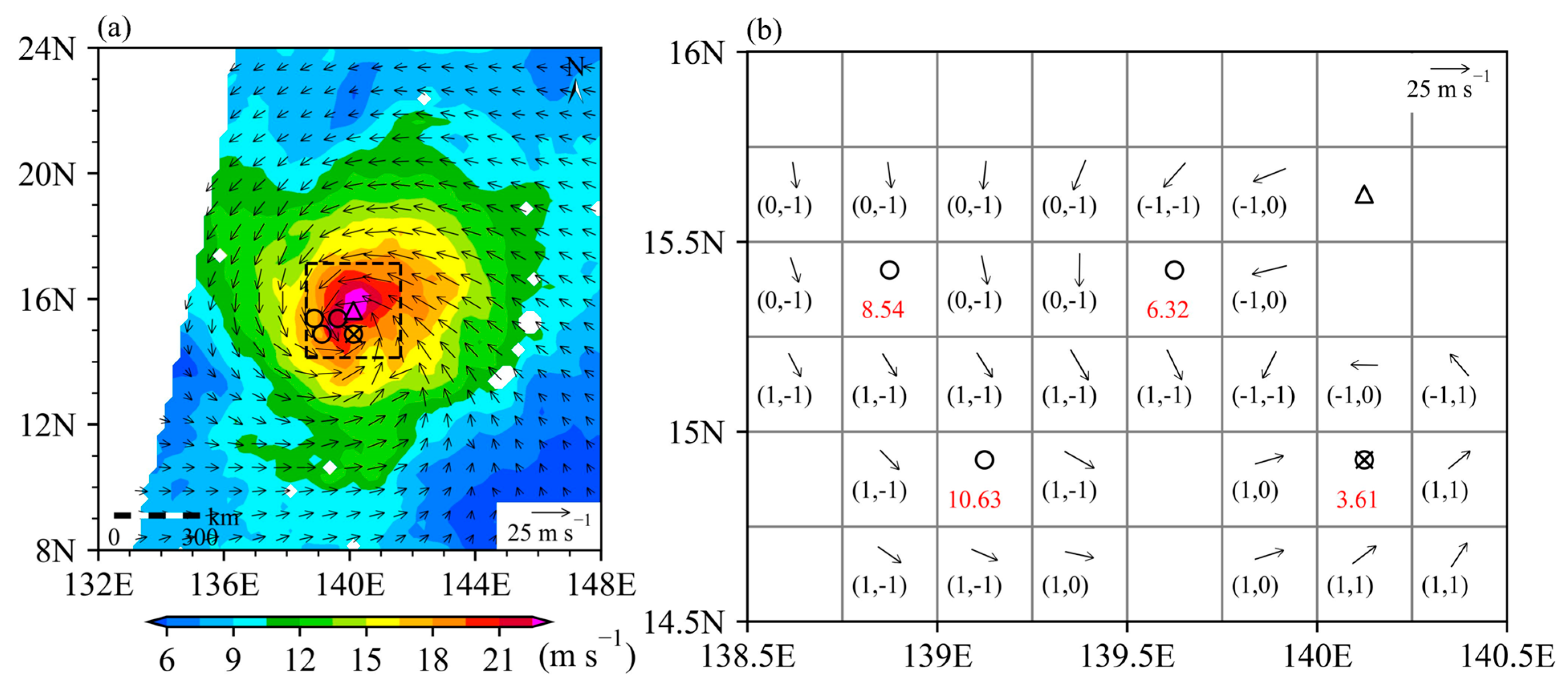
3.1. TC Center Positioning Method
- Find the max wind speed location (triangle).
- Within a 3° × 3° box, find all minimum wind speeds (circle) that are less than their immediate neighbors.
- Define eight two-component vectors at the eight nearest points around each wind-speed minimum: if the raw wind direction is within 0° ± 22.5°, 45° ± 22.5°, 90° ± 22.5°, 135° ± 22.5°, 180° ± 22.5°, 225° ± 22.5°, 270° ± 22.5°, and 315° ± 22.5°, the discrete vectors take the values of (1, 1), (1, 0), (1, −1), (0, −1), (−1, −1), (−1, 0), (−1, 1), and (0, 1), respectively.
- Compute the absolute sum of these eight direction vectors: .
- The minimum wind point with the smallest sum is the TC center (cross).
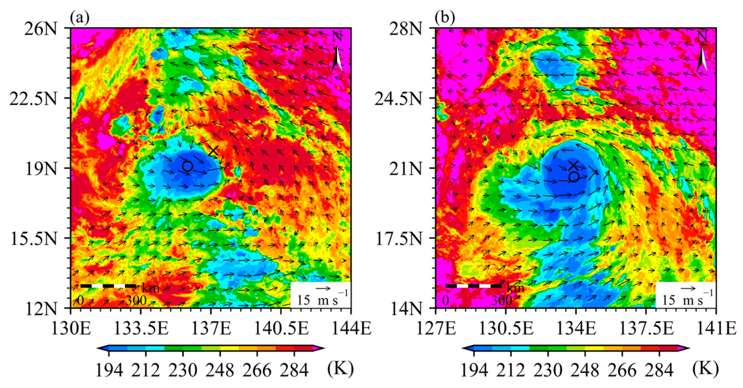
- Use the system-clustering method to identify three points with the lowest brightness temperature in the eyewall. The original channel-13 TB observations are averaged onto a 0.3° × 0.3° grid. The data points where TB observations are less than an empirical value of = 202 K are determined. Each of the data points is considered as an initial cluster. If there are N data points with TB observations being less than , there are N clusters. The two clusters with the closest minimum distance among the N clusters are merged together to form a new cluster. The new cluster is further merged with one of the remaining clusters whose distance from the new cluster is the smallest. This procedure is repeated until only the newest cluster and one remaining cluster are left. The three points of the minimum TB values in the newest cluster are identified for the next step.
- Fit a circle passing the three points identified by the cluster method; the circle center is the first guess.
- Perform an azimuthal spectral analysis for each grid in a 4° × 4° domain centered at the first guess point with 0.15° × 0.15° resolution, and the grid location leading to the largest wavenumber-0 amplitude is taken as a refined center over the guess point.
- Repeat the spectral analysis for each grid in a 2° × 2° domain centered at a refined center with 0.025° × 0.025° resolution, and the grid corresponding to the largest wavenumber-0 amplitude is taken as the final TC center.
3.2. Bogus Vortex Formula
3.3. Vertical Wind Shear
3.4. Case Description
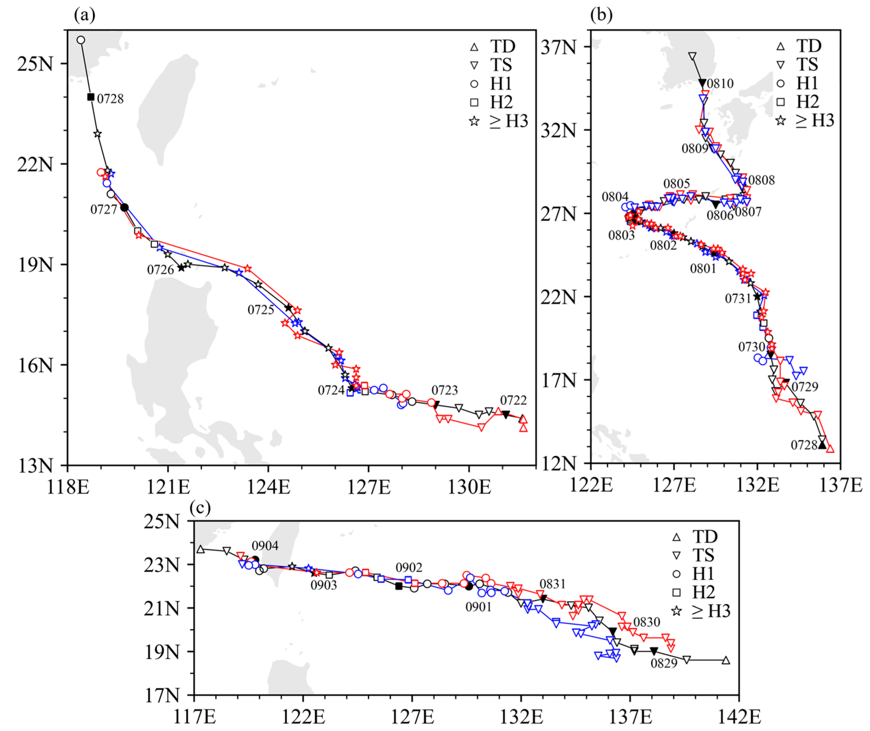
- Doksuri (5th typhoon in 2023 NW Pacific): Formed on 21 July east of the Philippines. Rapidly intensified (RI) before crossing Luzon and reached super typhoon status around 27 July (max wind ~62 m s−1). Made landfall around 28 July near Jinjiang, Fujian (~50 m s−1, 945 hPa), then moved north, with heavy rains. Weakened to depression by 29 July.
- Khanun (6th): Formed on 28 July and reached super typhoon strength around 31 July (935 hPa, 52 m s−1). Initially moved westward, turned northeast around 4 August in the East China Sea, then north. Landfall near Gyeongsangnam, South Korea on 10 August (28 m s−1, 975 hPa), and again near Liaoning, China on 11 August.
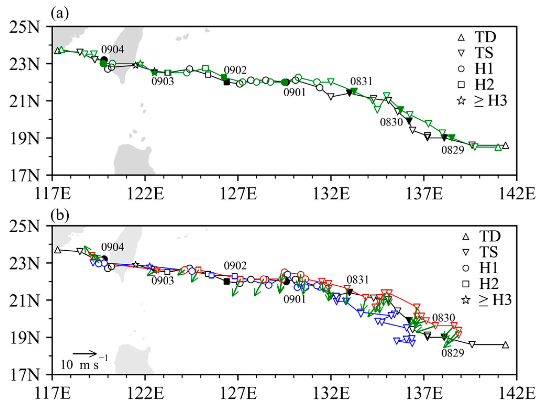
- Haikui (11th): Formed on 28 August, reached a severe tropical storm around 29 August, and became a typhoon by around 1 September. Landed in southeastern Taiwan on 3 September (~30 m s−1), and a second landfall on 5 September in Dongshan County, Fujian (~975 hPa).
4. Results
4.1. TC Center Positioning Results
4.2. Bogus Vortex Results
5. Discussion and Conclusions
Author Contributions
Funding
Data Availability Statement
Acknowledgments
Conflicts of Interest
Abbreviations
| POES | Polar-Orbiting Environmental Satellite |
| TC | Tropical cyclone |
| GOES | Geostationary environmental satellite |
| ERS | European Space Agency |
| MetOp | Meteorological operational satellite |
| NASA | National Aeronautics and Space Administration |
| CFOSAT | Chinese–French Oceanography Satellite |
| HY-2 | Hai Yang-2 |
| FY-3E | Fengyun-3E |
| ECMWF | European Centre for Medium-Range Weather Forecasts |
| AMI-SCAT | Active Microwave Instrument Scatterometer |
| ASCAT | Advanced scatterometer |
| SNR | Signal-to-noise ratio |
| GMF | Geophysical model function |
| WindRAD | Wind Radar |
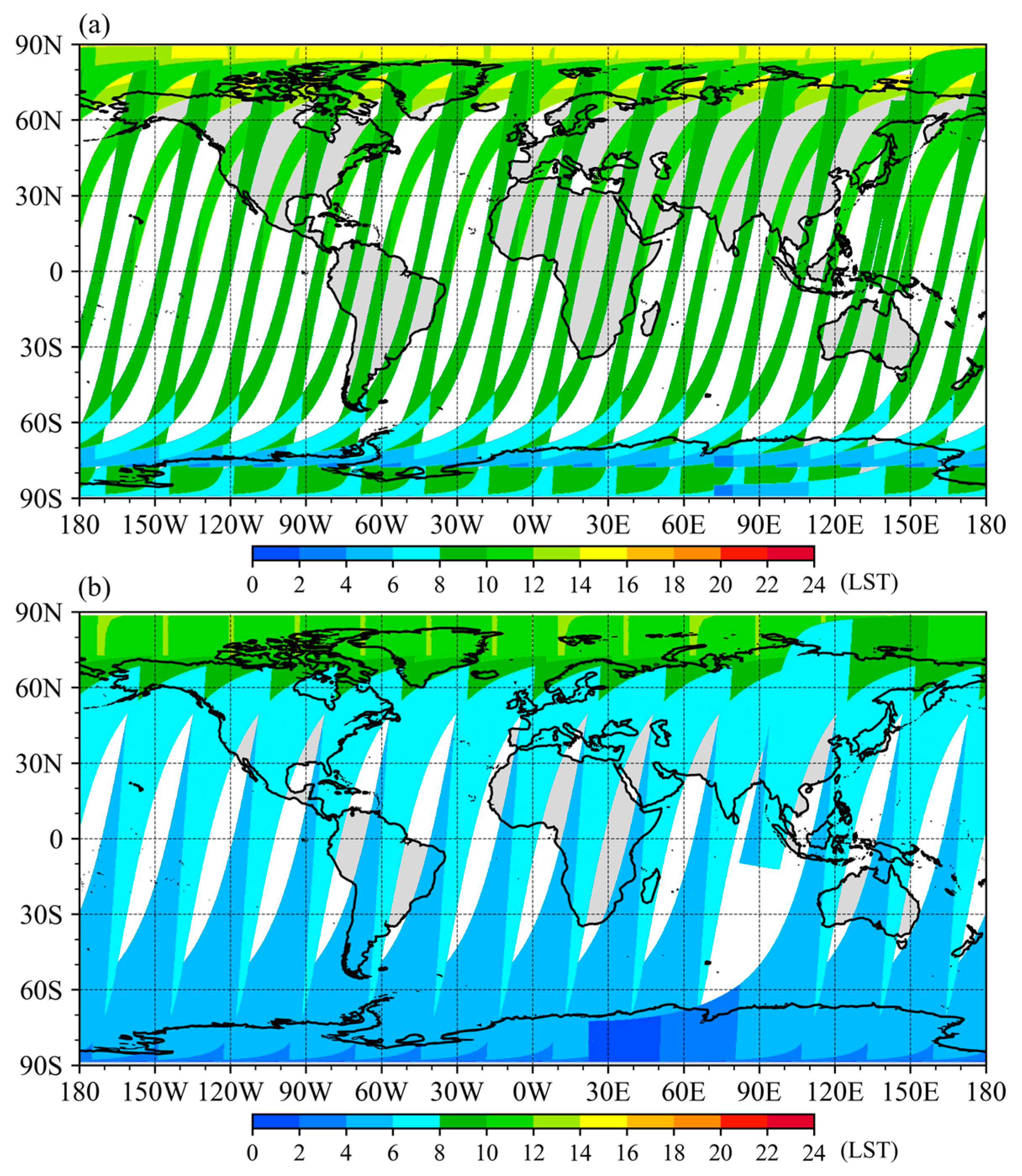
| LECT | Local equatorial crossing time |
| 4D-Var | Four-dimensional variation |
| UTC | Universal Time Coordinated |
| BDA | Bogus data assimilation |
| MM5 | Mesoscale Model version 5 |
| MTCSWA | Multi-platform Tropical Cyclone Surface Wind Analysis |
| NESDIS | National Environmental Satellite, Data, and Information Service |
| STAR | Satellite Application and Research |
| NOAA | National Oceanic and Atmospheric Administration |
| CLASS | Comprehensive Large Array-Data Stewardship System |
| IBTrACS | International Best Track Archive for Climate Stewardship |
| ICOADS | International Comprehensive Ocean-Atmosphere Data Set |
| IMMA | International Maritime Meteorological Archive |
| NRT | Near real time |
| ERA5 | Fifth Generation ECMWF Reanalysis |
| AHI | Advanced Himawari Imager |
| SLP | Sea level pressure |
| RI | Rapid intensification |
| ARCHER | Automated Rotational Center Hurricane Eye Retrieval |
| TC | Tropical cyclone |
| DOAJ | Directory of open access journals |
| TLA | Three letter acronym |
| LD | Linear dichroism |
| LST | Local Solar Time |
References
- Han, Y.; Revercomb, H.; Cromp, M.; Gu, D.; Johnson, D.; Mooney, D.; Scott, D.; Strow, L.; Bingham, G.; Borg, L.; et al. Suomi NPP CrIS measurements, sensor data record algorithm, calibration and validation activities, and record data quality. J. Geophys. Res. Atmos. 2013, 118, 12734–12748. [Google Scholar] [CrossRef]
- Lin, L.; Zou, X.; Weng, F. Combining CrIS double CO2 bands for detecting clouds located in different layers of the atmosphere. J. Geophys. Res. Atmos. 2017, 122, 1811–1827. [Google Scholar] [CrossRef]
- Xia, X.; Zou, X. Impacts of AMSU-A inter-sensor calibration and diurnal correction on satellite-derived linear and nonlinear decadal climate trends of atmospheric temperature. Clim. Dyn. 2020, 54, 1245–1265. [Google Scholar] [CrossRef]
- Weng, F.; Zou, X.; Wang, X.; Yang, S.; Goldberg, M.D. Introduction to Suomi national polar-orbiting partnership advanced technology microwave sounder for numerical weather prediction and tropical cyclone applications. J. Geophys. Res. Atmos. 2012, 117, D19112. [Google Scholar] [CrossRef]
- Zou, X.; Weng, F.; Zhang, B.; Lin, L.; Qin, Z.; Tallapragada, V. Impacts of assimilation of ATMS data in HWRF on track and intensity forecasts of 2012 four landfall hurricanes. J. Geophys. Res. Atmos. 2013, 118, 11558–11576. [Google Scholar] [CrossRef]
- Bi, M.; Zou, X. Comparison of cloud/rain band structures of Typhoon Muifa (2022) revealed in FY-3E MWHS-2 observations with all-sky simulations. J. Geophys. Res. Atmos. 2023, 128, e2023JD039410. [Google Scholar] [CrossRef]
- Wu, Q.; Chen, G. Validation and intercomparison of HY-2A/MetOp-A/Oceansat-2 scatterometer wind products. Chin. J. Oceanol. Limnol. 2015, 33, 1181–1190. [Google Scholar] [CrossRef]
- Gray, W.M.; Neumann, C.; Tsui, T.L. Assessment of the role of aircraft reconnaissance on tropical cyclone analysis and forecasting. Bull. Am. Meteorol. Soc. 1991, 72, 1867–1883. [Google Scholar] [CrossRef]
- de Kloe, J.; Stoffelen, A.; Verhoef, A. Improved use of scatterometer measurements by using stress-equivalent reference winds. IEEE J. Sel. Top. Appl. Earth Obs. Remote Sens. 2017, 10, 2340–2347. [Google Scholar] [CrossRef]
- Grantham, W.; Bracalente, E.; Jones, W.; Johnson, J. The Seasat-A satellite scatterometer. IEEE J. Ocean. Eng. 1977, 2, 200–206. [Google Scholar] [CrossRef]
- Naderi, F.; Freilich, M.; Long, D. Spaceborne radar measurement of wind velocity over the ocean-an overview of the NSCAT scatterometer system. Proc. IEEE 1991, 79, 850–866. [Google Scholar] [CrossRef]
- Bell, B.; Thépaut, J.-N.; Eyre, J. The assimilation of satellite data in numerical weather prediction systems. In Satellites for Atmospheric Sciences 2: Meteorology, Climate and Atmospheric Composition; Wiley: Hoboken, NY, USA, 2023; pp. 69–95. [Google Scholar] [CrossRef]
- Sankhala, D.K.; Rani, S.I.; Srinivas, D.; Prasad, V.; George, J.P. Validation of OceanSat-3 sea surface winds for their utilization in the NCMRWF NWP assimilation systems. Adv. Space Res. 2024, 75, 1945–1959. [Google Scholar] [CrossRef]
- Fujita, T. Pressure distribution within typhoon. Geophys. Mag. 1952, 23, 437–451. [Google Scholar]
- Holland, G.J. An analytic model of the wind and pressure profiles in hurricanes. Mon. Weather Rev. 1980, 108, 1212–1218. [Google Scholar] [CrossRef]
- Bjerknes, V. On the Dynamics of the Circular Vortex: With Applications to the Atmosphere and Atmospheric Vortex and Wave Motions; (No. 4); I kommission hos Cammermeyers bokhandel; Cammermeyers Bokhandel: Oslo, Norway, 1921. [Google Scholar]
- Takahashi, K. Distribution of pressure and wind in a typhoon. J. Meteorolog. Soc. Jpn. 1939, 17, 417–421. [Google Scholar]
- Zou, X.; Xiao, Q. Studies on the initialization and simulation of a mature hurricane using a variational bogus data assimilation scheme. J. Atmos. Sci. 2000, 57, 836–860. [Google Scholar] [CrossRef]
- Van Nguyen, H.; Chen, Y.-L. High-resolution initialization and simulations of Typhoon Morakot (2009). Mon. Weather Rev. 2011, 139, 1463–1491. [Google Scholar] [CrossRef]
- Xiao, Q.; Kuo, Y.-H.; Zhang, Y.; Barker, D.M.; Won, D.-J. A tropical cyclone bogus data assimilation scheme in the MM5 3D-Var system and numerical experiments with typhoon rusa (2002) near landfall. J. Meteorol. Soc. Jpn. 2006, 84, 671–689. [Google Scholar] [CrossRef]
- Yu, C.; Yang, Y.; Yin, X.; Sun, M.; Shi, Y. Impact of Enhanced wave-induced mixing on the ocean upper mixed layer during typhoon Nepartak in a regional model of the Northwest Pacific Ocean. Remote Sens. 2020, 12, 2808. [Google Scholar] [CrossRef]
- Park, K.; Zou, X. Toward developing an objective 4DVAR BDA scheme for hurricane initialization based on TPC observed parameters. Mon. Weather Rev. 2004, 132, 2054–2069. [Google Scholar] [CrossRef]
- Hu, T.; Wu, Y.; Zheng, G.; Zhang, D.; Zhang, Y.; Li, Y. Tropical cyclone center automatic determination model based on HY-2 and QuikSCAT wind vector products. IEEE Trans. Geosci. Remote Sens. 2019, 57, 709–721. [Google Scholar] [CrossRef]
- Zhang, C.; Zou, X.; Tan, Z.-M. Eye and eyewall radii and track of Typhoon Trami (2018) derived from advanced himawari imager (AHI) brightness temperature observations. IEEE Trans. Geosci. Remote Sens. 2023, 61, 4104311. [Google Scholar] [CrossRef]
- Bhate, J.; Munsi, A.; Kesarkar, A.; Kutty, G.; Deb, S.K. Impact of assimilation of satellite retrieved ocean surface winds on the tropical cyclone simulations over the north Indian Ocean. Earth Space Sci. 2021, 8, e2020EA001517. [Google Scholar] [CrossRef]
- Kattamanchi, V.K.; Viswanadhapalli, Y.; Dasari, H.P.; Langodan, S.; Vissa, N.K.; Sanikommu, S.; Rao, S.V.B. Impact of assimilation of SCATSAT-1 data on coupled ocean-atmospheric simulations of tropical cyclones over Bay of Bengal. Atmospheric Res. 2021, 261, 105733. [Google Scholar] [CrossRef]
- Stiles, B.W.; Portabella, M.; Yang, X.; Zheng, G. Editorial for Special Issue “Tropical Cyclones Remote Sensing and Data Assimilation”. Remote Sens. 2020, 12, 3067. [Google Scholar] [CrossRef]
- Eyre, J.R.; English, S.J.; Forsythe, M. Assimilation of satellite data in numerical weather prediction. Part I: The early years. Q. J. R. Meteorol. Soc. 2020, 146, 49–68. [Google Scholar] [CrossRef]
- Fetterer, F.; Gineris, D.; Wackerman, C. Validating a scatterometer wind algorithm for ERS-1 SAR. IEEE Trans. Geosci. Remote Sens. 1998, 36, 479–492. [Google Scholar] [CrossRef]
- Huddleston, J.; Spencer, M. SeaWinds: The QuikSCAT wind scatterometer. In Proceedings of the 2001 IEEE Aerospace Conference Proceedings (Cat. No. 01TH8542), Big Sky, MT, USA, 10–17 March 2001; pp. 41825–41831. [Google Scholar] [CrossRef]
- Figa-Saldaña, J.; Wilson, J.J.W.; Attema, E.; Gelsthorpe, R.; Drinkwater, M.R.; Stoffelen, A. The advanced scatterometer (ASCAT) on the meteorological operational (MetOp) platform: A follow on for European wind scatterometers. Can. J. Remote Sens. 2002, 28, 404–412. [Google Scholar] [CrossRef]
- Zhang, Y.; Lin, M.; Song, Q. Evaluation of geolocation errors of the Chinese HY-2A satellite microwave scatterometer. IEEE Trans. Geosci. Remote Sens. 2018, 56, 6124–6133. [Google Scholar] [CrossRef]
- Zhang, Y.; Lin, M.; Xie, X.; Mu, B.; Wang, X.; Lang, S. The improvement of HY-2 Satellite’s Microwave Scatterometer instrument and NRCS calculation. IEEE Trans. Geosci. Remote Sens. 2024, 62, 5112109. [Google Scholar] [CrossRef]
- Qin, D.; Jia, Y.; Lin, M.; Liu, S. Performance evaluation of China’s first ocean dynamic environment satellite constellation. Remote Sens. 2023, 15, 4780. [Google Scholar] [CrossRef]
- Niu, Z.; Zou, X. Improving all-sky simulations of Typhoon cloud/rain band structures of NOAA-20 CrIS window channel observations. J. Geophys. Res. Atmos. 2024, 129, e2023JD040622. [Google Scholar] [CrossRef]
- Shang, J.; Wang, Z.; Dou, F.; Yuan, M.; Yin, H.; Liu, L.; Wang, Y.; Hu, X.; Zhang, P. Preliminary performance of the WindRAD scatterometer onboard the FY-3E meteorological satellite. IEEE Trans. Geosci. Remote Sens. 2024, 62, 5100813. [Google Scholar] [CrossRef]
- Knaff, J.A.; DeMaria, M.; Molenar, D.A.; Sampson, C.R.; Seybold, M.G. An automated, objective, multiple-satellite-platform tropical cyclone surface wind analysis. J. Appl. Meteorol. Clim. 2011, 50, 2149–2166. [Google Scholar] [CrossRef]
- Knaff, J.A.; Slocum, C.J. An automated method to analyze tropical cyclone surface winds from real-time aircraft reconnaissance observations. Weather Forecast. 2024, 39, 333–349. [Google Scholar] [CrossRef]
- Freeman, E.; Woodruff, S.D.; Worley, S.J.; Lubker, S.J.; Kent, E.C.; Angel, W.E.; Berry, D.I.; Brohan, P.; Eastman, R.; Gates, L.; et al. ICOADS Release 3.0: A major update to the historical marine climate record. Int. J. Clim. 2017, 37, 2211–2232. [Google Scholar] [CrossRef]
- Knapp, K.R.; Kruk, M.C.; Levinson, D.H.; Diamond, H.J.; Neumann, C.J. The international best track archive for climate stewardship (IBTrACS) unifying tropical cyclone data. Bull. Am. Meteorol. Soc. 2010, 91, 363–376. [Google Scholar] [CrossRef]
- Hersbach, H.; Bell, B.; Berrisford, P.; Hirahara, S.; Horányi, A.; Muñoz-Sabater, J.; Nicolas, J.; Peubey, C.; Radu, R.; Schepers, D.; et al. The ERA5 global reanalysis. Q. J. R. Meteorol. Soc. 2020, 146, 1999–2049. [Google Scholar] [CrossRef]
- DeMaria, M. The effect of vertical shear on tropical cyclone intensity change. J. Atmos. Sci. 1996, 53, 2076–2088. [Google Scholar] [CrossRef]
- DeMaria, M.; Mainelli, M.; Shay, L.K.; Knaff, J.A.; Kaplan, J. Further Improvements to the Statistical Hurricane Intensity Prediction Scheme (SHIPS). Weather Forecast. 2005, 20, 531–543. [Google Scholar] [CrossRef]
- Gray, W.M. Global view of the origin of tropical disturbances and storms. Mon. Weather Rev. 1968, 96, 669–700. [Google Scholar] [CrossRef]
- Wimmers, A.J.; Velden, C.S. Objectively determining the rotational center of tropical cyclones in passive microwave satellite imagery. J. Appl. Meteorol. Clim. 2010, 49, 2013–2034. [Google Scholar] [CrossRef]
- Wimmers, A.J.; Velden, C.S. Advancements in objective multisatellite tropical cyclone center fixing. J. Appl. Meteorol. Clim. 2016, 55, 197–212. [Google Scholar] [CrossRef]
- Dvorak, V.F. Tropical cyclone intensity analysis and forecasting from satellite imagery. Mon. Weather Rev. 1975, 103, 420–430. [Google Scholar] [CrossRef]
- Tuttle, J.; Gall, R. A single-radar technique for estimating the winds in tropical cyclones. Bull. Am. Meteorol. Soc. 1999, 80, 653–668. [Google Scholar] [CrossRef]
- Frank, W.M.; Ritchie, E.A. Effects of vertical wind shear on the intensity and structure of numerically simulated hurricanes. Mon. Weather Rev. 2001, 129, 2249–2269. [Google Scholar] [CrossRef]


Disclaimer/Publisher’s Note: The statements, opinions and data contained in all publications are solely those of the individual author(s) and contributor(s) and not of MDPI and/or the editor(s). MDPI and/or the editor(s) disclaim responsibility for any injury to people or property resulting from any ideas, methods, instructions or products referred to in the content. |
© 2025 by the authors. Licensee MDPI, Basel, Switzerland. This article is an open access article distributed under the terms and conditions of the Creative Commons Attribution (CC BY) license (https://creativecommons.org/licenses/by/4.0/).
Share and Cite
Pan, W.; Zou, X.; Duan, Y. Developing an Objective Scheme to Construct Hurricane Bogus Vortices Based on Scatterometer Sea Surface Wind Data. Remote Sens. 2025, 17, 1528. https://doi.org/10.3390/rs17091528
Pan W, Zou X, Duan Y. Developing an Objective Scheme to Construct Hurricane Bogus Vortices Based on Scatterometer Sea Surface Wind Data. Remote Sensing. 2025; 17(9):1528. https://doi.org/10.3390/rs17091528
Chicago/Turabian StylePan, Weixin, Xiaolei Zou, and Yihong Duan. 2025. "Developing an Objective Scheme to Construct Hurricane Bogus Vortices Based on Scatterometer Sea Surface Wind Data" Remote Sensing 17, no. 9: 1528. https://doi.org/10.3390/rs17091528
APA StylePan, W., Zou, X., & Duan, Y. (2025). Developing an Objective Scheme to Construct Hurricane Bogus Vortices Based on Scatterometer Sea Surface Wind Data. Remote Sensing, 17(9), 1528. https://doi.org/10.3390/rs17091528