Detecting Post-Midnight Plasma Depletions Through Plasma Density and Electric Field Measurements in the Low-Latitude Ionosphere

Abstract

Plasma depletions in the low-latitude ionosphere are irregularities of special interest in space weather research, as they are highly detrimental to the operation of satellite-based communication and navigation systems. In this frame, we present the results of a systematic study of the low-latitude topside ionosphere, based on in situ measurements of both electron density ($N_e$) and electric field provided by the Langmuir Probe (LP) and the Electric Field Detector (EFD) onboard the first China Seismo-Electromagnetic Satellite (CSES-01). Specifically, by exploiting in situ measurements from 1 January 2019 to 31 May 2024, we devised two different techniques for the automatic detection of post-midnight plasma depletions at about 500 km of altitude: one using only $N_e$ observations, the other using only electric field measurements. We validated these new techniques against each other and performed a statistical investigation of the main characteristics of the observed plasma irregularities, such as their latitudinal extension, longitudinal distribution, and monthly and seasonal occurrence. To test the robustness and reliability of our algorithms, we also applied them to well-established Swarm B satellite observations. In particular, we first investigated both the monthly and the seasonal occurrences of post-sunset plasma depletions detected between 18:00 and 04:00 local time (LT), by LP onboard the Swarm B satellite at about 500 km of altitude. In addition, we compared ionospheric irregularities detected by Swarm B with those detected by CSES-01. For the comparison, we considered Swarm B LP data collected for the same period as the CSES-01 dataset and under the same conditions by selecting Swarm B observations in the range 01:00 $\le LT<$ 03:00. Our results prove the robustness and reliability of both LP and EFD algorithms in detecting plasma depletions, and their good agreement suggests their complementarity in detecting such kinds of plasma irregularities. Results also confirm consistency between CSES-01 and Swarm B observations (once the same LT orbits have been considered) and with the relevant literature on the topic.

1. Introduction

The post-sunset ionosphere at low magnetic latitudes is highly susceptible to instabilities, which allow plasma density irregularities to develop. At local dusk, indeed, the absence of sunlight leads to a much faster ionospheric recombination at lower altitudes with respect to higher ones, thus causing the establishment of steep upward plasma density gradients, which in turn result in the growth of the collision-dominated Rayleigh-Taylor (R-T) instability (see, e.g., [1,2,3]). This process triggers the formation of plasma-depleted regions at the bottom side of the F-layer, which then rise buoyantly upwards to the top side of the F-layer [4,5]. Generally, these irregularities occur within a narrow band of $\pm {20}^{°}$ of magnetic latitude, where they align with the geomagnetic field, stretching hundreds of kilometers in the magnetic north–south direction [6,7]. Most of such depletions have a favored scale size near 100 km [8], but they may have spatial extents between 150 km and 450 km [9,10], evolving as single or multiple structures.

The importance of equatorial plasma depletions (hereafter, we use the nomenclature Equatorial Plasma Bubble (EPB) for such irregularities to align with the literature on the topic) relies on their capability in affecting many modern-day technologies, especially those dependent on space-based navigation systems, such as the Global Navigation Satellite System (GNSS), which transmit on the L-band (see, e.g., [11,12]). Since the ionosphere acts as a propagation medium, such irregularities may cause disturbances in both the phase and the amplitude of radio signals. In severe cases, they can also lead to the loss of signal lock when the ground-based receiver tries to record the signal from a satellite as it enters the field of view [13,14,15,16,17]. Therefore, EPBs remain an important component of space weather and continue to be studied vigorously even after many decades since their existence was discovered.

Traditional diagnostic methods of EPBs exploit various instruments, including ionogram traces obtained from ionosonde observations [18,19], coherent and incoherent scatter radars (e.g., [20,21,22]), airglow imagers (e.g., [22,23,24]), in situ rocket- and satellite-based measurements (e.g., [25,26,27,28,29,30]), and GNSS observations (e.g., [31,32,33,34,35]). Such methods have allowed the assessment of the main mechanisms for generating post-sunset plasma bubbles, including their multiscale temporal variability, such as long-term variability mainly due to solar cycle dependencies and medium-term variability mainly induced by seasonal variations (see reviews by [36,37,38]). However, mechanisms for generating the post-midnight irregularities are still unknown and extensively debated.

In this context, the CSES mission provides unique sun-synchronous observations to address important questions on post-midnight EPBs variability. The availability of measurements from both the LP and the EFD onboard CSES-01 offers the opportunity for conducting a new systematic study of the statistical properties of post-midnight ionospheric depletions. In this work, we present two new techniques for the automatic detection of post-midnight plasma depletions, one using LP data and the other using EFD data. We validate these techniques by performing a statistical analysis of a 4-year LP nighttime dataset, where we analyze EPBs’ climatology in terms of spatial extension, latitudinal and longitudinal occurrence, and seasonal dependence. Moreover, by exploiting Swarm B LP data collected for the same period as the CSES-01 dataset, we test the reliability of the proposed techniques in catching both post-sunset and post-midnight plasma bubbles.

This paper is structured as follows: Section 2 provides an overview of the data considered here and detailed descriptions of both the LP and the EFD algorithms developed to automatically detect EPBs. Section 3 discusses the results of the statistical analysis performed on the 4-year LP nighttime dataset. Finally, Section 4 provides a summary and conclusions.

2. Data and Methods

2.1. Data

CSES-01 is a scientific mission dedicated to monitoring electromagnetic fields and plasma variations in the topside ionosphere, as induced by natural sources and anthropogenic emissions, and to study their possible correlations with the occurrence of seismic events [39]. CSES-01, launched on 2 February 2018 and still in operation, orbits sun-synchronously at an altitude of ∼500 km, with an orbital period of ∼94 min and an inclination of $97.4^{°}$. It has an average speed of ∼7.2 km/s, descending and ascending nodes at ∼14:00 LT and ∼02:00 LT, respectively, and a revisit period of 5 days. CSES-01 carries a full suite of instruments for measuring the ionospheric electromagnetic fields and plasma properties, among which, as used in the present study, the LP and the EFD.

The LP, designed for in situ measurements of bulk parameters of the ionospheric plasma, provides continuous measurements of the electron density ($N_e$) and temperature ($T_e$) between $5\times {10}^2{\mathrm{cm}}^{-3}$ and $1\times {10}^7{\mathrm{cm}}^{-3}$ and between 500 K and 10,000 K, respectively, both with an accuracy of $10\%$ [40,41] and a sampling frequency of 3 s in survey mode.

The EFD is designed to take measurements of the ionospheric vector electric field in several frequency bands. More specifically, in the Extremely Low Frequency (ELF) band [42,43] used in this work, EFD provides continuous measurements with a sampling frequency of 5 kHz. Measurements of all instruments onboard CSES-01 are taken continuously only between $-{65}^{°}$ and $+{65}^{°}$ of geographic latitude due to telemetry constraints.

The Swarm constellation, launched at the end of 2013 and still in operation, consists of three low-Earth-orbit satellites that provide high-precision and high-resolution measurements of the amplitude, direction, and variation in magnetic field and plasma properties (such as temperature and ion density [44,45,46]).

The Swarm satellites are located at two different quasi-circular polar orbits, two flying side-by-side at an initial altitude of 460 km (Swarm A and C), and the third one flying at an initial altitude of 530 km (Swarm B). Unlike CSES-01, Swarm satellites drift in LT, covering a full 24 h LT cycle in about 130–140 days. Swarm LPs provide continuous measurements of ion density ($N_i$) and electron temperature ($T_e$) at a sampling frequency of 2 Hz in harmonic mode [47]. At the Swarm satellite’s altitude, the plasma quasi-neutrality is so well verified that it is safe to assume $N_i\simeq N_e$ and compare the CSES-01 $N_e$ with the Swarm B $N_i$. For the present work, we analyzed the $N_i$ data acquired by Swarm B LP, orbiting roughly at the same altitude as CSES-01 during the analyzed period (2019–2024), downsampled to $1/3$ Hz to allow a better comparison with the CSES-01 LP data. Despite the plethora of calibrations and corrections recently delivered about Swarm LP observations [48,49,50,51,52,53], we decided to use the original LP observations because the algorithm for the EPBs identification does not depend on the absolute magnitude of LP observations, but on the ratios with respect to a baseline calculated from actual observations themselves.

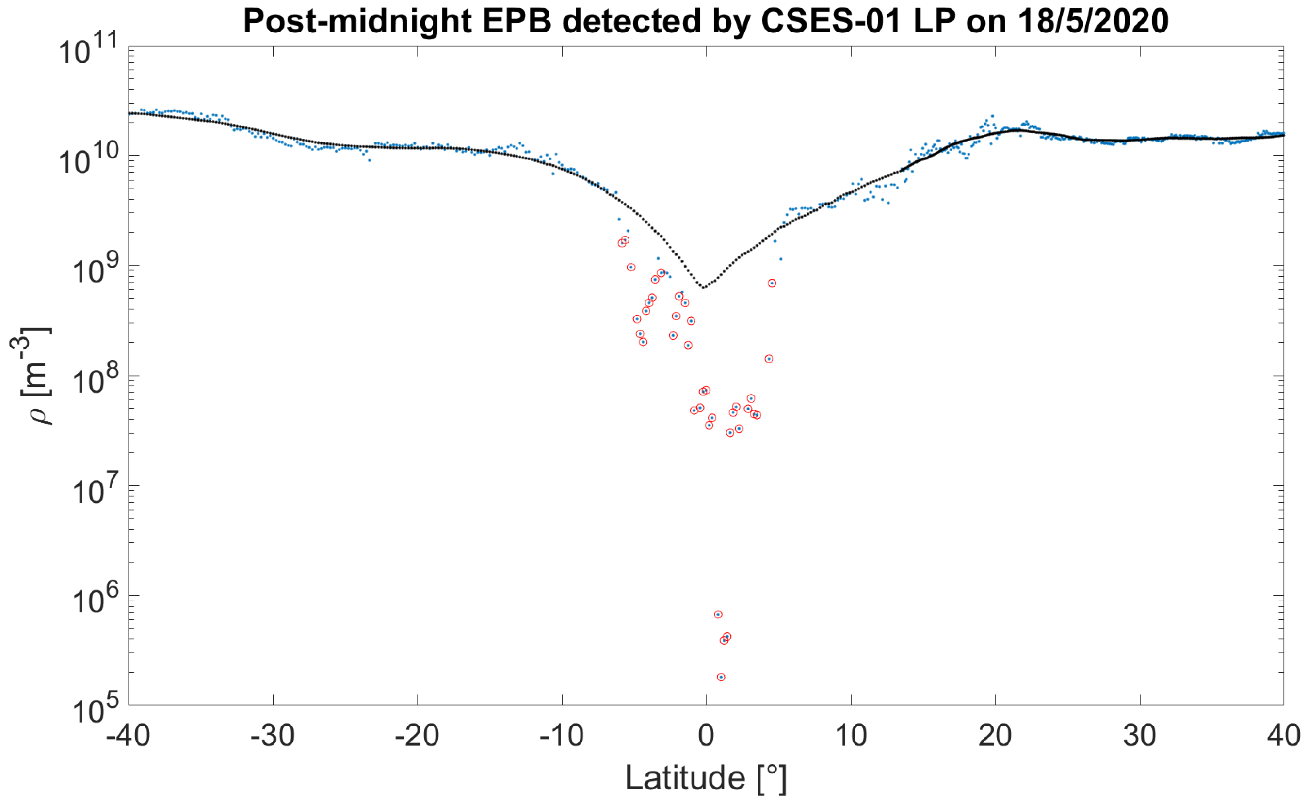
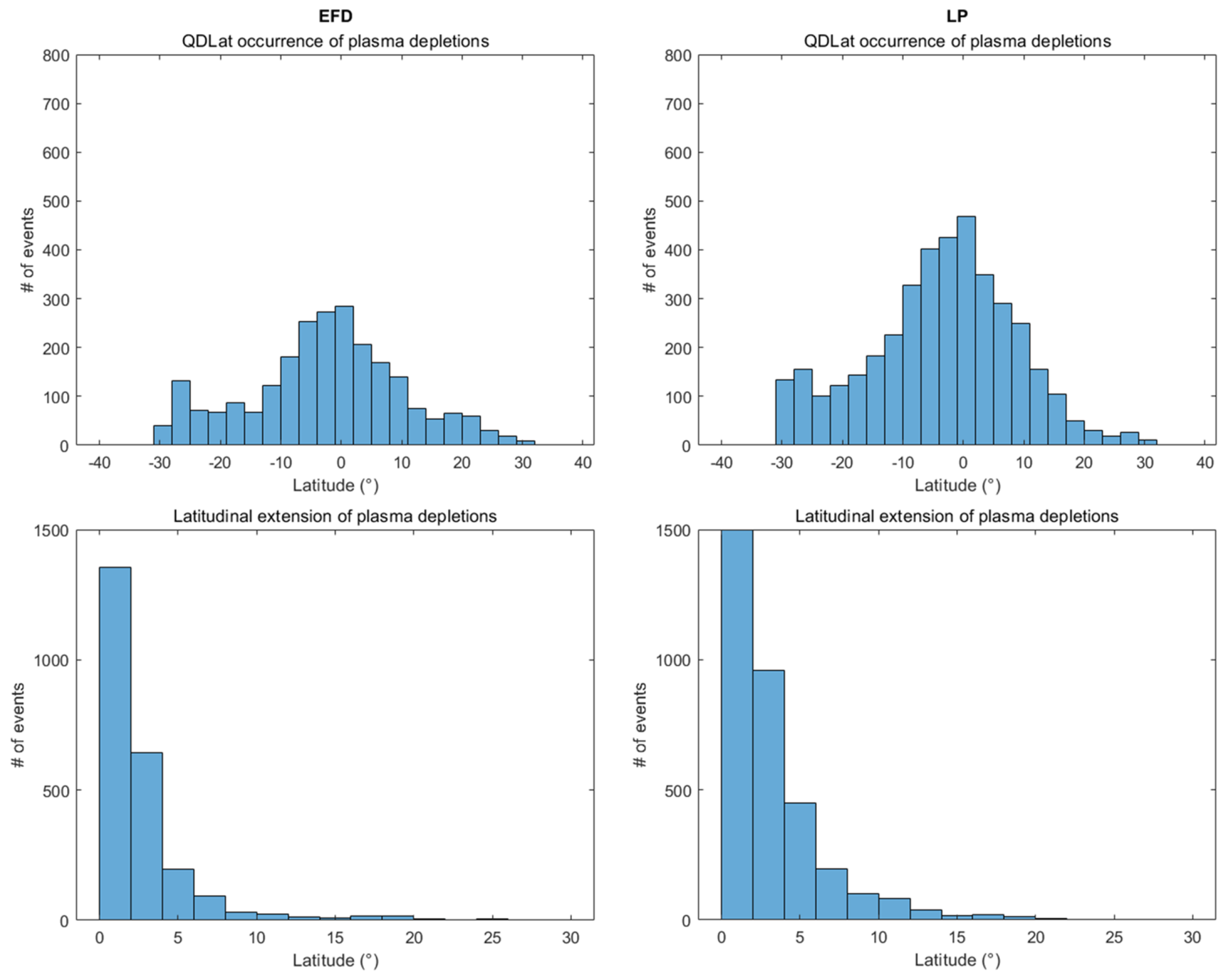
2.2. EPB Detection Based on LP Measurements of Plasma Density

To automatically detect EPBs, we devised and developed an algorithm based on in situ LP measurements, which works as follows.

For each orbit, we consider the timeseries of theplasma density measurements $n_s$ from LP ($s=e$ for electron density measurements by CSES-01 and $s=i$ for ion density measurements by Swarm B) and compute the density baseline according to the following equation:

$${\tilde{n}}_s\left(t_k\right)={\displaystyle \frac{1}{57}}\sum _{j=k-28}^{k+28}{n}_s\left(t_k\right),$$

(1)

where k denotes the kth point of the timeseries. We use a running mean with a window size larger than the maximum expected size of an equatorial ionospheric irregularity (see e.g., [54]). Specifically, given the temporal resolution of our datasets (see Section 2.1), this corresponds to taking a running mean with a window size of 57 points, corresponding to ∼170 s or 1200 km (transformed using the average orbital velocity of CSES-01 and Swarm B, i.e., 7.2 km/s). We then take the density ratio with respect to the baseline $\delta n_s=n_s\left(t_k\right)/{\tilde{n}}_s\left(t_k\right)$ and, in order for a given interval to contain a plasma depletion, we impose the following conditions:

• The ratio $\delta n_s$ between the density measured at each point along the semiorbit and the running mean of the density is less than 1/2;
• The above condition is satisfied for at least five points along the semiorbit;
• Points whose time distance is lower than 40 s are considered as belonging to the same depletion; otherwise, they are considered as belonging to two (or more) different depletions.
• Identified intervals are located in a latitudinal band from −30° to 30° of quasi dipole magnetic latitude [55].

The first condition allows identifying any abrupt density decrease along the orbit. Since we are interested in detecting EPBs, whose density is significantly reduced compared with the background (see, e.g., [38,56] and references therein), we define a plasma depletion as a region where the plasma density is less than half that of the surrounding plasma. This condition also agrees with [57], who, in order to automatically detect polar cap patches (see, e.g., [58]) using ion density data from LP onboard Swarm satellites, imposes that the ratio between the foreground density and the background density is greater than 2. This threshold guarantees to consider irregularities whose density gradient is able to disturb HF radio propagation and degrade GNSS signals (see, e.g., [59]). For this reason, we extend this definition also to ionospheric irregularities in equatorial regions.

The second condition ensures that the detected density decreases are not due to any sporadic fluctuations. The minimum interval length has been chosen based on visual inspection of several orbits, resulting in a good compromise between excluding random fluctuations while concurrently being able to identify scale irregularities on the order of tens of kilometers.

Imposing a time difference greater than 40 s between two consecutive detected intervals containing depletions allows for a better estimation of the number of plasma depletions detected along the orbit. Such a condition, indeed, ensures to correctly count multiple plasma depletions that eventually occur along a semiorbit, also evaluating whether plasma fragmentation occurs inside a plasma bubble. Such an interval has been chosen based on visual inspection of several orbits as the best trade-off between the possibility of considering fragmentation of large structures and of maintaining information about the nature of the detected irregularity.

The last condition allows for investigating only depletions occurring at low latitudes.

All imposed thresholds reduce the number of false positive detections to less than 10%, the latter being mainly linked to the inability of the moving average to follow the density profile in cases of failure of the LP data acquisition. We remark that due to the imposed thresholds, the algorithm, by design, is unable to detect false negatives (unlike for the EFD algorithm, see Section 2.3). The estimation of the percentage of false positive events was obtained by visual inspection of all the semiorbits in one year in which the algorithm detected EPBs (327 in 2019), then counting the number of failures (2 in 2019).

Once a plasma depletion has been identified, the algorithm saves the information related to both the orbit (date and orbit number) and the ionospheric irregularities (start and end time of the density decrease, its starting/ending geographic and quasi-dipole latitude and longitude). Figure 1 shows the EPB automatically detected by the LP algorithm along the ascending semiorbit 12716 of CSES-01 on 18 May 2020. In this case, the LP algorithm detected a single depletion.

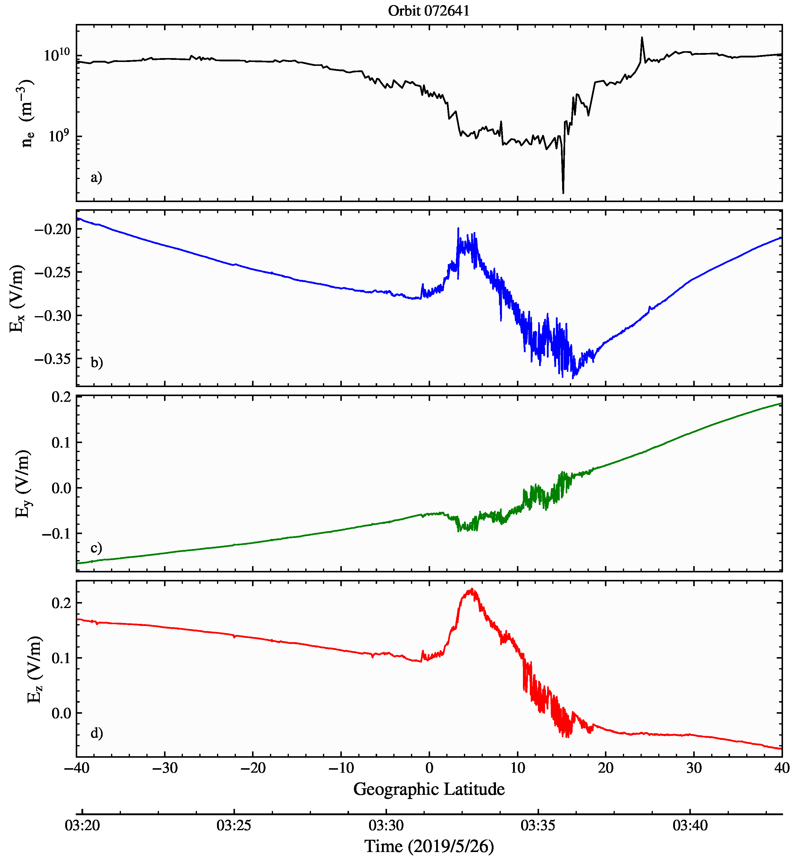
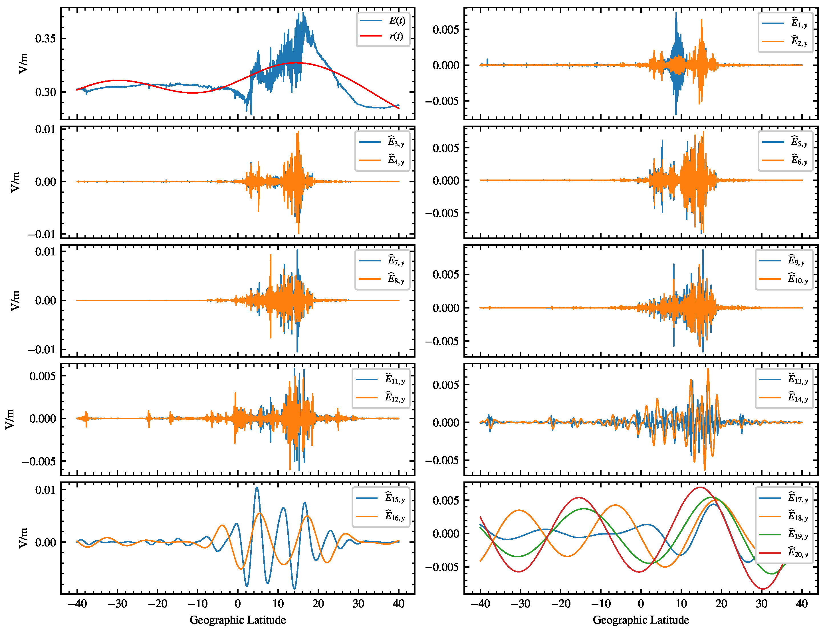
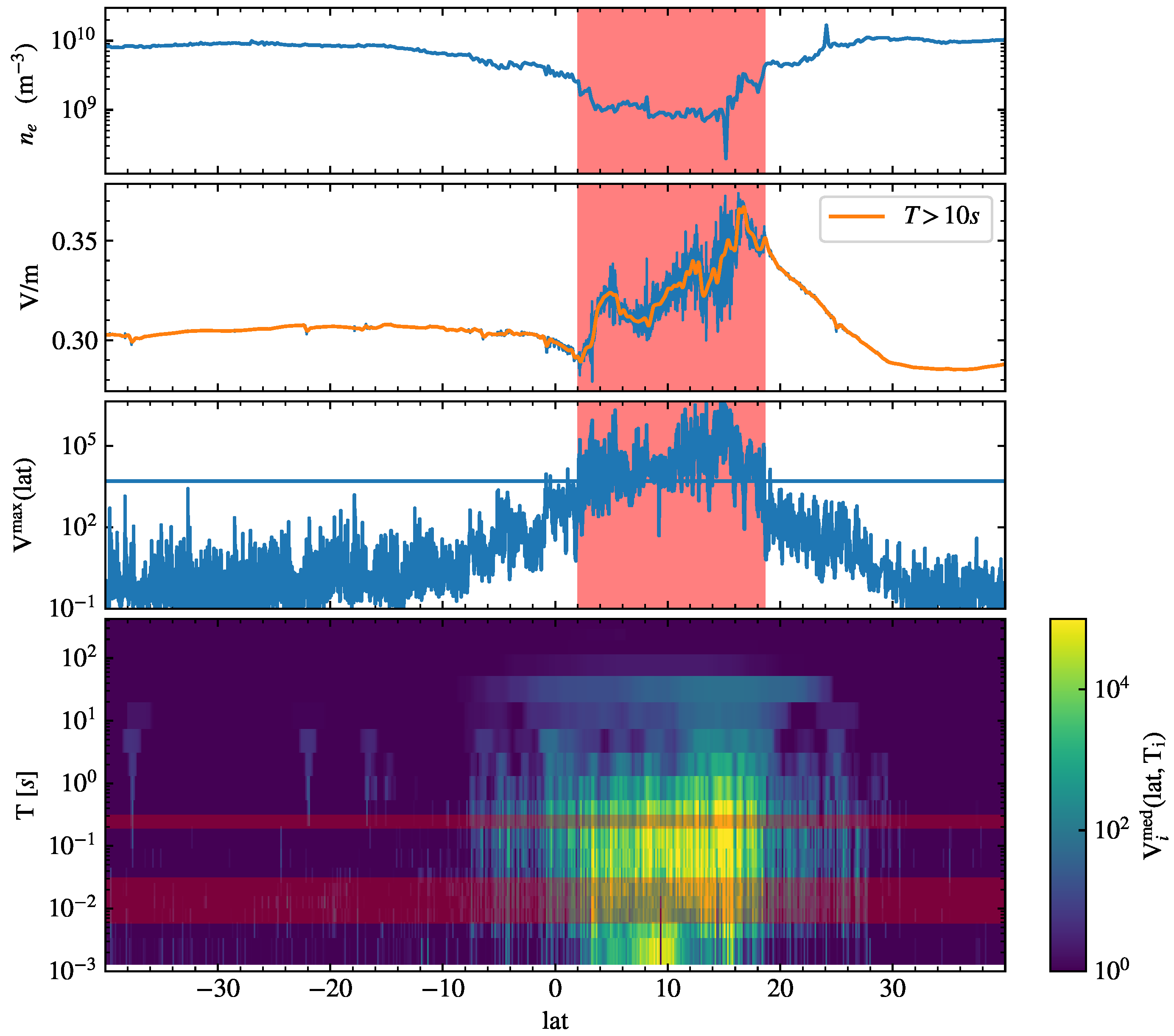
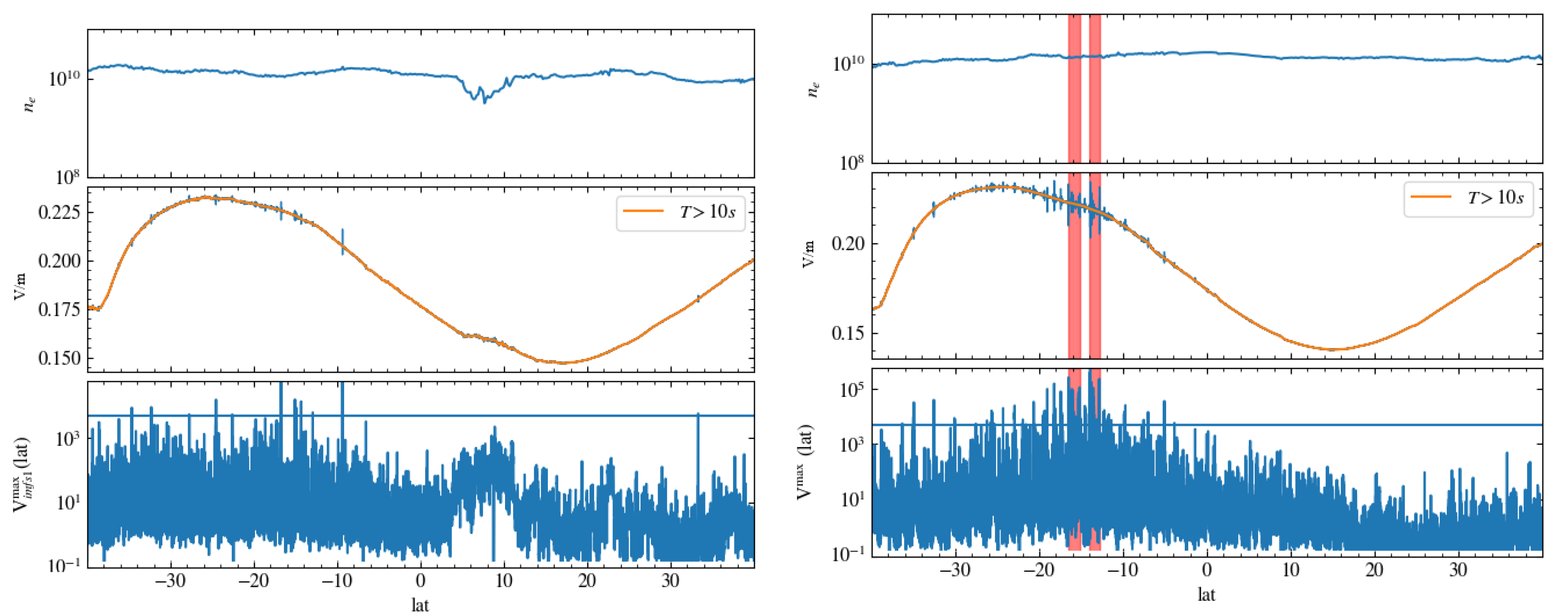
2.3. EPB Detection Based on a Local Variance Measure of the Electric Field

When CSES-01 flies through an equatorial irregularity, the electric field fluctuations increase significantly in a broadband spectrum of frequencies. The observation of such a spread of electric power over a wide range of frequencies is likely generated by the turbulent convection embedded within the plasma depletion; see, e.g., [6,7,60,61,62,63]. In Figure 2, we show an example of such a signal recorded by CSES-01 during a crossing of an EPB. In that figure, concurrently with a decrease in the electron density (panel a), an energy increase in the electric field fluctuations is observed in all components (panels b–d).

We identify such a multiscale increase as the signature of the crossing of an irregularity by CSES-01.

Such a signal shares many similarities with the multifrequency electric field fluctuations observed at auroral latitudes (generated by intense field-aligned currents) that we investigated in [64]. In that work, a new method was devised for the automatic detection of the crossing of the Auroral Oval (AO) by CSES-01 based on the multiscale characterization of the electric field activity. The detection was made by means of a clustering thresholding algorithm applied to a measure of the multiscale relative energy of the electric field.

Building on those results, we modified the AO detection algorithm of [64] to allow detecting the crossing of EPBs by CSES-01 by means of electric field measurements only. The modified algorithm relies on Fast Iterative Filtering (FIF) [65] to perform a decomposition of the amplitude of the electric field and uses the Median-Weighted Local Variance Measure (hereafter MWLVM [64]) to calculate a proxy of the electric field activity. FIF is designed to decompose a nonstationary nonlinear signal into a set of Intrinsic Mode Components (IMCs) that oscillate around zero with varying amplitude and frequency, plus a residual or trend. FIF is similar to the Empirical Mode Decomposition (EMD) technique developed by [66], but with an important difference in the calculation of the moving average. Indeed, EMD removes the low-frequency component from a given signal by means of spline interpolation of the signal envelope (defined by the relative extrema of the signal), while FIF convolves the signal with a Fokker-Planck (low-pass) filter function. Such a difference led to the demonstration of the a priori convergence of FIF [67]. Once the proxy has been calculated, a clustering algorithm is applied to identify the crossing of the EPB by CSES-01. We refer to the overall procedure as the EFD detection algorithm. The main difference with respect to the original AO detection algorithm [64] is the use of the electric field amplitude as input dataset in place of the full vector electric field (and consequently the use of FIF in place of Multivariate FIF [68]). In the following, other differences will be highlighted if needed.

To better describe all the steps of the algorithm, we employ the dataset in Figure 2 as a reference. For any semiorbit in the night-side, we take EFD measurements of the electric field in the Extreme-Low-Frequency (ELF) band, in an equatorial latitudinal band below/above $\pm {30}^{°}$ of quasi-dipole magnetic latitude, and calculate the electric field amplitude $E\left(t\right)=\sqrt{E_x^2\left(t\right)+E_y^2\left(t\right)+E_z^2\left(t\right)}$. Here, we always express all quantities as a function of time t. However, we note that most of the plots use the geographic (or quasi-dipole) latitude in place of t, by exploiting the one-to-one correspondence between the two variables (see Figure 2).

We then apply the FIF decomposition and obtain a set of IMCs ${\widehat{E}}_i\left(t\right)$, such that

$$E\left(t\right)=\sum _{i=1}^M{\widehat{E}}_i\left(t\right)+r\left(t\right),$$

(2)

where $r\left(t\right)$ is the residual trend of the decomposition, and M is the number of extracted IMCs. Figure 3 shows an example of such decomposition.

The third step consists in the calculation of the MWLVM of the set $\left\{{\widehat{E}}_i\right\}$, defined as

$${\mathrm{V}}_i^{\mathrm{med}}(t,T_i)={\displaystyle \frac{{\mathrm{V}}_i(t,T_i)}{\mathrm{med}{\left\{{\mathrm{V}}_i(t,T_i)\right\}}_t}},$$

(3)

where $\mathrm{med}{\left\{\cdots \right\}}_t$ denotes the median operator and

$${\mathrm{V}}_i(t,T_i)={\displaystyle \frac{1}{N_i}}\sum _{\tau =t-T_i/2}^{t+T_i/2}{\left({\widehat{E}}_i\left(\tau \right)-{\mu }_i(t,T_i)\right)}^2$$

(4)

is the moving variance of ${\widehat{E}}_i\left(t\right)$ over a sliding window of length $T_i$, that corresponds to the length of the kernel function of the low-pass filter used by FIF to extract the i-th IMC. Here, ${\mu }_i$ is the moving mean of ${\widehat{E}}_i$ and $N_i$ is the number of points contained in the time interval $T_i$, i.e., $N_i=T_i/dt$, $dt$ being the sampling time of EFD, in this case $dt=2\times {10}^{-3}\mathrm{s}$ (we note that, by design of the FIF decomposition, $T_i$ is always an integer multiple of $dt$, and so is $N_i$).

The bottom panel of Figure 4 shows a colored contour of ${\mathrm{V}}_i^{\mathrm{med}}$ obtained from EFD measurements of the reference dataset. The broadband signal due to the presence of the EPB is evident. We then define our activity proxy

$${\mathrm{V}}^{max}\left(t\right)=\underset{T_i\in \mathbb{A}}{max}\left\{{\mathrm{V}}_i^{\mathrm{med}}(t,T_i)\right\},\mathbb{A}=[0.006\mathrm{s},0.03\mathrm{s}]\cup [0.2\mathrm{s},0.3\mathrm{s}],$$

(5)

where the range $\mathbb{A}$ (denoted by red horizontal stripes in bottom panel of Figure 4) is chosen so as to retain a spatial accuracy of ∼2 km (i.e., ∼$0.{16}^{°}$ in latitude) and, at the same time, avoid both spurious systematic signals introduced by the instrument and instrumental/ambient noise at high frequencies. A plot of ${\mathrm{V}}^{max}$ is shown in Figure 4.

The final step of the detection procedure consists in the application of the same clustering algorithm used in [64], but with a few modifications to the parameters employed. More specifically, we set the following:

• A threshold of 5000 on the activity proxy ${\mathrm{V}}^{max}$;
• A minimum latitudinal extension of $1^{°}$ for the fluctuations above the threshold;
• A minimum distance between two consecutive intervals of $0.4^{°}$ (below this value, intervals are merged together).

As for the LP detection algorithm (see Section 2.2), the choice of the above values has been made to reduce the percentage of false positives, so as to maximize the performance of the detection. The constraint on the minimum latitudinal extension corresponds to setting a lower limit of roughly 120 km on the size of the interval, while the last constraint means that we consider as the same EPB two intervals which are separated by less than 48 km. The choice of the lower limit ensures, on one hand, that the typical scale size of EPBs [8] is captured by the EFD algorithm. Concurrently, on the other hand, such a choice minimizes statistical fluctuations in the MWLVM, since 120 km corresponds to roughly 80.000 points of EFD ELF data. The intervals returned by the clustering algorithm are identified as crossing of an EPB by the spacecraft. As an example, the vertical red stripes in the three upper panels of Figure 4 denote the latitudinal extension of the detected EPB.

The EFD algorithm has been run on the EFD-ELF dataset available from 2019 to 2024 and on the night side semiorbits (consistently with the LP dataset selection). The performance of the algorithm has been assessed by visual inspection of 515 sample semiorbits, randomly picked from the dataset. For this sample, the algorithm returned a correct answer for 454 semiorbits (corresponding to >88% of the sample), consisting of 26 positive and 428 negative detections. In addition, the algorithm returned 35 false positive detections (out of the 61 wrong answers), corresponding to a rate of false positive detections of $57\%$, if one considers only positive detections. Both false positive and negative detections are mainly caused by transients in the ionospheric electric field, such as, e.g., whistler events. For instance, in Figure 5, we report an erroneous negative detection (left panel) returned by the EFD algorithm. A plasma depletion (clearly present at a latitude of ${10}^{°}$) causes an increase in the activity proxy, which, however, is below the threshold. This is due to the presence of transient induced electric activity between $-{30}^{°}$ and $-{10}^{°}$, which increases the median value of the electric field variance ${\mathrm{V}}_i(t,T_i)$ (see Equation (4)), thus decreasing the value of MWLVM and, consequently, the value of ${\mathrm{V}}^{max}$. At the same time, strong transient events can be misidentified as EPBs. This is the case shown in the right panel of the same figure.

3. Results and Discussion

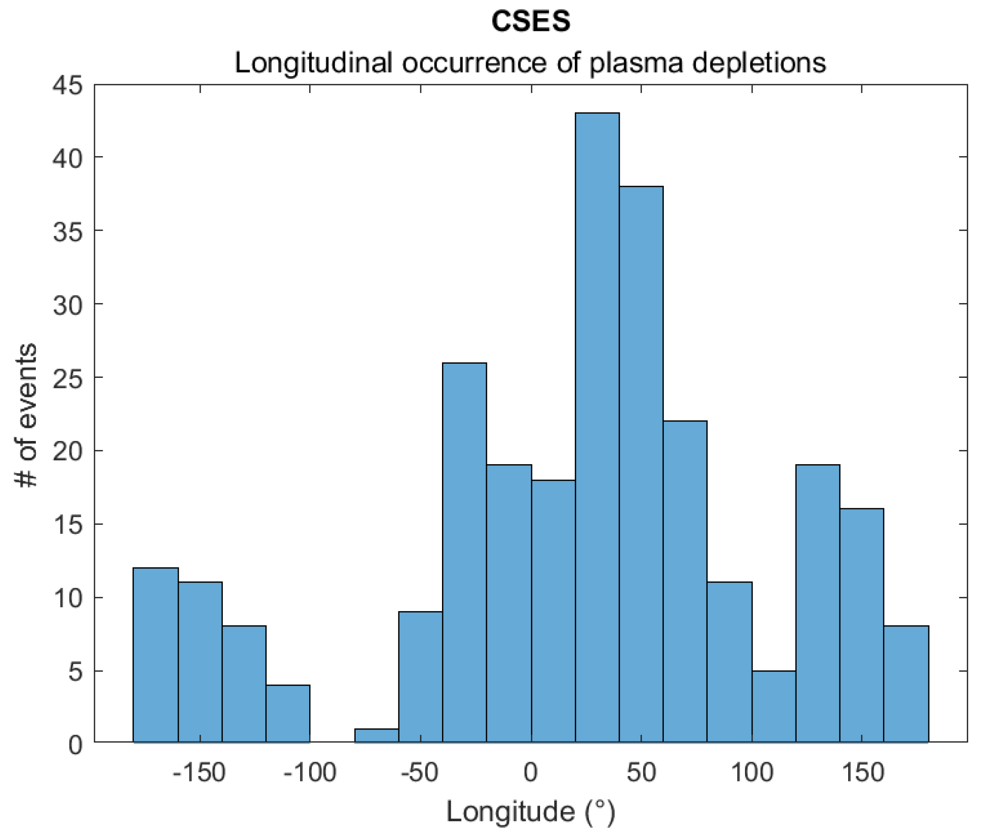
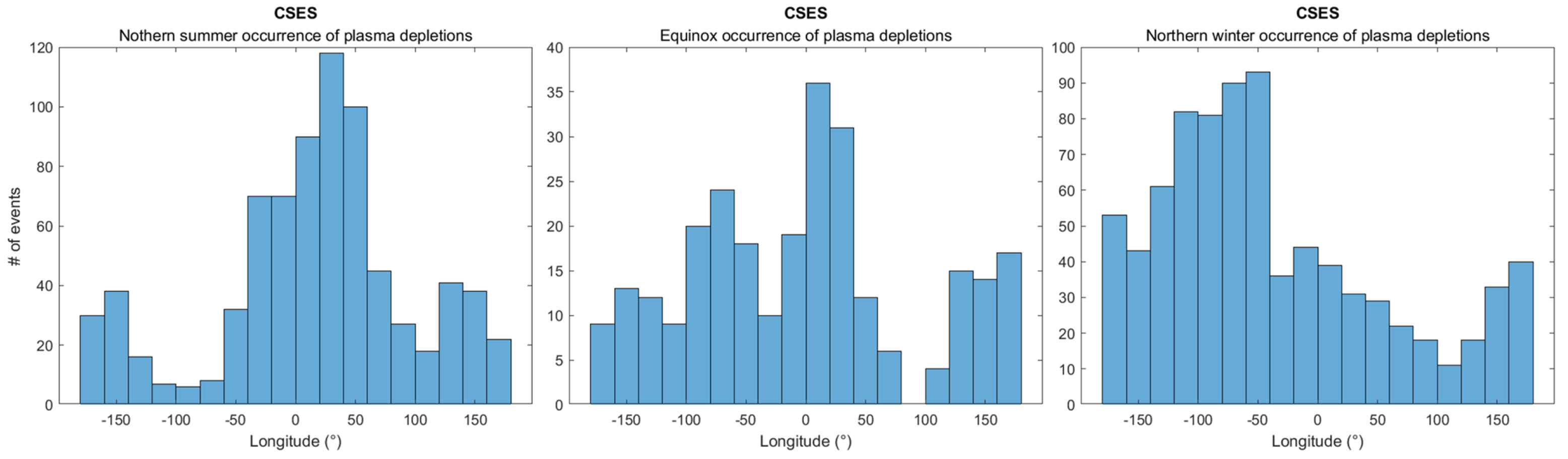
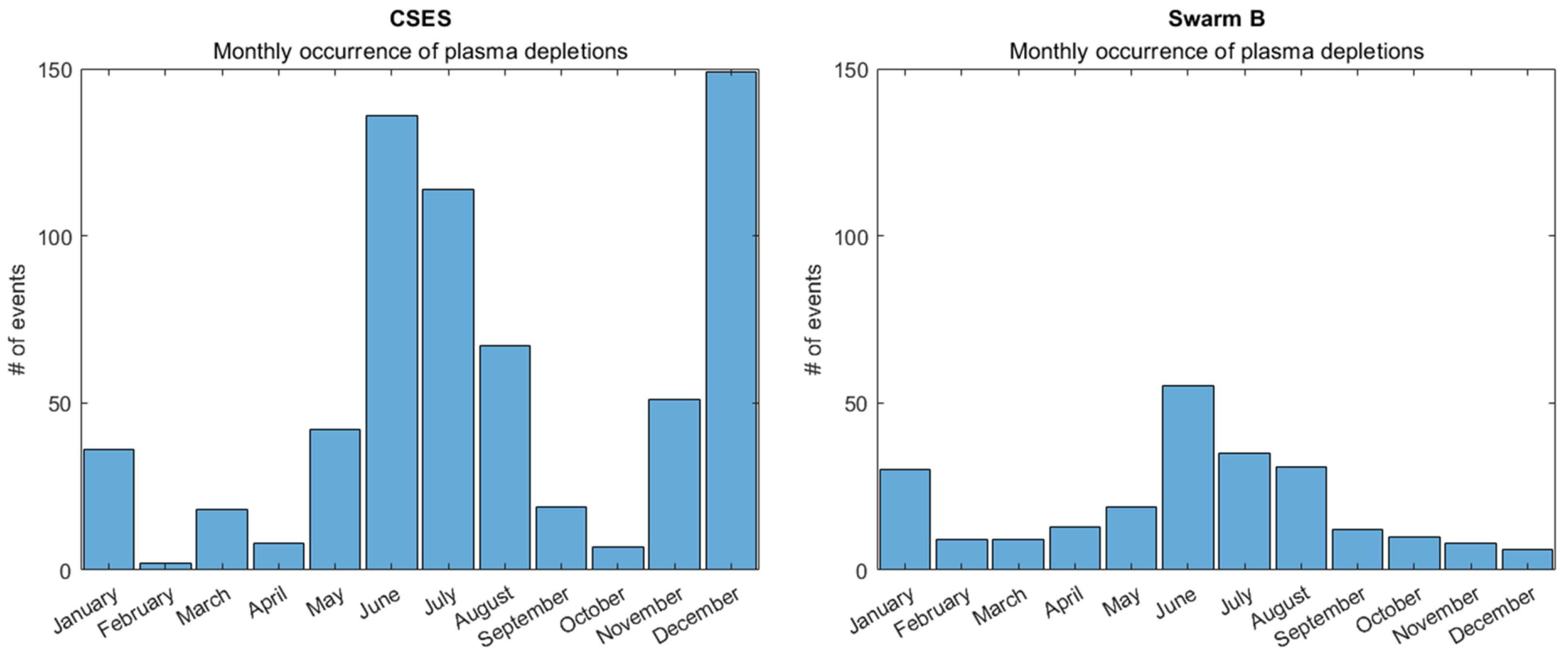
3.1. Post-Midnight EPBs from CSES-01 Observations

Table 1. Number of EPBs automatically detected from 1 January 2019 to 31 May 2024, by LP and EFD onboard CSES-01. The table also reports the number of semiorbits in which EPBs are detected.

Instrument	Number of Detected EPBs	Number of Semiorbits
LP	3973	1937
EFD	2411	1598
LP ∩ EFD	1658	800

summarizes the number of EPBs automatically detected from 1 January 2019 to 31 May 2024 by both the LP and the EFD algorithms, together with the number of semiorbits in which at least one EPB was detected. It is worth noting that the two algorithms do not detect the same number of ionospheric irregularities. This is essentially due to the differences between LP and EFD measurements, which, as described in Section 2.2 and Section 2.3, resulted in the need to adopt different proxies and independent thresholds to optimize the automatic detection. The higher number of irregularities detected by the LP algorithm compared with EFD is mainly due to its ability to count even smaller irregularities (see points 2 and 3 in Section 2.2), which usually occur inside a plasma bubble (see, e.g., [69] and reference therein). Furthermore, the EFD saturation effect, which could occur in correspondence with intense depletions (<10⁸ m⁻³; see [70]), makes the electric field measurement less reliable to reveal the presence of electric field fluctuations in correspondence with strong EPBs.

By comparing the irregularities identified by EFD with those identified by LP, it is observed that the semiorbits of the common detections (last column in Table 1) represent ∼41.3% of the entire LP dataset. Based on the above arguments, one would expect such a percentage to be much higher (around $80\%$ accounting for algorithms’ performance), since by design, EFD detections should be a subset of LP detections. This apparent discrepancy is explained by the fact that the estimated rate of false positive detections of the EFD algorithm is ∼57% (see Section 2.3), while for the LP algorithm, it is less than $10\%$. Therefore, out of the 1598 semiorbits of positive detection reported for EFD, only half are true detections, which correspond roughly to the number of common semiorbits.

As discussed in the previous Section (also visible in Figure 5), the proxy used for the EPBs detection using EFD data is sensitive to electric field variations, eventually associated with other physical phenomena (such as whistlers). In any case, common detection from the EFD and LP algorithms allows for investigating the electric field dynamics of EPBs. In addition, the false positive detections (identified by the combined use of the two algorithms) can be exploited to investigate other physical phenomena.

By investigating the latitudinal extension and the latitudinal occurrence (see Figure 6) of detected irregularities, we found that most of them have an extension within $1000$ km (bottom panels) and occur within a narrow band of $\pm {20}^{°}$ of quasi-dipole magnetic latitude (top panels). These results suggest a good agreement between the two algorithms, highlighting their complementarity in identifying these types of ionospheric irregularities.

The goodness of these results is also confirmed by the monthly EPBs occurrence distributions detected by the two algorithms, as shown in Figure 7. As visible by comparing left and right panels, showing LP (left) and EFD (right) EPBs occurrences, respectively, both algorithms detected the largest number of equatorial irregularities during the solstice months. This result agrees well with previous studies, which reported an increased occurrence of post-midnight EPBs during solstice periods of low solar activity (e.g., [71,72,73,74]). In particular, Heelis et al. [75], analyzing ion density perturbations based on measurements made by the Communication/Navigation Outage Forecasting System (C/NOFS) satellite, pointed out that the maximum in the occurrence rate of irregularities across midnight into the post-midnight hours takes place during the June and December solstices. In addition, Otsuka et al. [76] and Nishioka et al. [77] noted that Field-Aligned Irregularities (FAI) echoes from 2006 to 2010, associated with EPBs, appeared more frequently after midnight between May and August. Since, differently from previous studies, the period under investigation also covers the rising phase of Solar Cycle 25, we tested the goodness of our results by investigating the monthly distribution of the occurrence of quiet days evaluated accordingly [78]. As in Figure 8, the main occurrence of quiet days was recorded during June, December, and January, suggesting that EPBs recorded by CSES-01 occur primarily during quiet days.

Following the results of Yizengaw et al. [79], reporting 4-year statistics (2009–2012) for post-midnight irregularities observed with the C/NOFS satellite, and indicating that the rate of occurrence of such irregularities peaks predominantly in the African sector during the June solstice, we investigated the regional dependence of EPBs during all June solstices covered by the present study. Our results, shown in Figure 9, agree well with those of [79]; in fact, the rate of occurrence of EPBs detected by the CSES-01 LP as a function of geographic longitude peaks predominantly in the African sector. According to the authors [79], this behavior could be attributed to the abundant appearance of the ionospheric sporadic E layer (Es) in the June solstice, which in turn could be a source of eastward electric field that leads to bubble formation during the local time after midnight.

In accordance with the results of Dao et al. [80], who studied plasma density variations retrieved by the C/NOFS satellite, we investigated the longitudinal occurrence of post-midnight EPBs separated by seasons. Figure 10 shows the longitudinal occurrence of EPBs automatically detected from 1 January 2019 to 31 May 2024 by CSES-01 LP during northern summer (left), equinox months (center), and northern winter (right). As seen in the figure, during northern summer (left), EPBs peak predominantly in the Atlantic-African sector; differently, during northern winter (right), the major occurrence rate was found in correspondence with the mid-Pacific and the American sectors. At the equinoxes, EPBs seem to mostly affect both the American and the African sectors. The longitudinal structures in which these irregularities occur are very similar to those reported by [80], suggesting that the lower atmospheric tides may have actively contributed to EPB formations.

Our results support findings of previous studies (see, e.g., [81] and references therein) and suggest that possible mechanisms for generating observed post-midnight irregularities could be both attributed to the seeding of the Rayleigh–Taylor instability by atmospheric gravity waves (propagating from below into the ionosphere) and, subsequently, to the uplift of the F layer induced by the meridional neutral winds in the thermosphere.

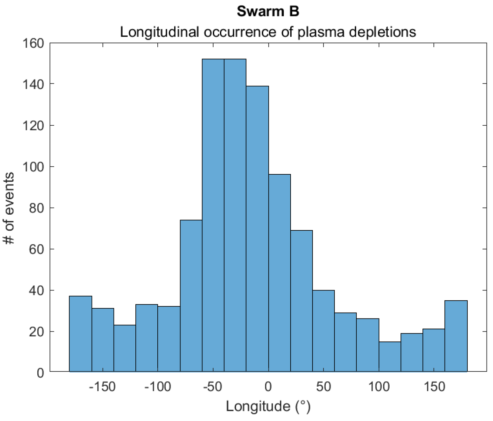
3.2. EPBs from Swarm B Observations

In order to test the reliability and robustness of our algorithms, we ran the algorithm based on in situ LP observations (see Section 2.2) on the ion density measurements acquired by the LP onboard the Swarm B satellite. Specifically, following the result of [82], we concentrated on orbits in the 18:00–04:00 LT sector, investigating all post-sunset EPBs detected from 1 January 2019 to 31 May 2024. The longitudinal occurrence in Figure 11 shows that a large number of post-sunset EPBs are found above the American–Atlantic–African sector, as also reported in previous studies (see, e.g., [82,83]). In addition, the investigation of the longitudinal distribution of post-sunset EPBs, in Figure 12, shows a clear seasonal dependence of the occurrence rate of such irregularities. Specifically, for equinox seasons (center panel), events occur in all longitude bins, with a clear preference for the Atlantic (∼−50^° E) and African (∼−20^° E) regions. A lower number of EPBs is detected for the summer season (left panel). Such irregularities in summer are concentrated mainly in the African-Atlantic regions. During this season, almost no events were observed in the Atlantic and the Indian sectors (∼100^° E). In contrast, a very high number of EPBs (>90) is reported in winter over the Atlantic sector (right panel) with respect to the other seasons. The rates decrease rapidly west and east of the Atlantic Ocean, and very few EPBs are detected over the Pacific. Such distributions agree well with what has been previously reported (see, e.g., [82,84,85]).

Cross-Validation Between Swarm B and CSES-01

With the aim to cross-validate Swarm B and CSES-01 observations, we also compared plasma depletions detected by the LP onboard Swarm B with those detected by the LP onboard CSES-01. In this frame, we considered the Swarm B LP data collected for the same period as the CSES-01 dataset and, according to what reported by Pignalberi et al. [52], we selected Swarm B observations in the range 01:00 $\le LT<$ 03:00. We then limited the search for EPBs in the CSES-01 database only to the months in which Swarm B and CSES-01 LT range overlapped. Figure 13 shows the monthly occurrences of EPBs detected from 1 January 2019 to 31 May 2024, both by CSES-01 (left) and Swarm B (right) LPs. As is visible, CSES-01 (left) detected on average more EPBs than Swarm B (right). Furthermore, the highest number of irregularities is recorded in June and December by CSES-01, while in June and January by Swarm B. These differences could be ascribed to the different orbital configuration of the two satellites. Indeed, while CSES-01 scans always the same LTs, Swarm B collects data in the CSES-01 LTs range only occasionally. This difference affects the monthly occurrence distribution of EPBs among the two satellites because Swarm B does not uniformly sample the different months at CSES-01 LTs. The monthly occurrence distribution in Figure 13 agrees well with the widely accepted evidence that EPBs occur frequently when the solar terminator is parallel to the geomagnetic field (see, e.g., [19,31,86]).

Despite the presence of these differences, by looking at Figure 13, it is possible to notice a good agreement between the two distributions. Indeed, both panels show how both satellites record the greatest occurrence in the northern summer months. This result is once again in agreement with what was previously described (see Section 3.1), underlining the reliability of our algorithm to identify these types of ionospheric irregularities. Furthermore, the goodness of these results highlights the great versatility of this algorithm, whose good performance is independent of the type of LP used.

4. Summary and Conclusions

In this paper, we introduced two new algorithms for plasma depletions detection that rely, respectively, on in situ measurements of the electric field and the electron density collected by the CSES-01 satellite in the topside ionosphere. The algorithms presented in this work have been designed to automatically detect plasma irregularities, such as the plasma depletions affecting the low-latitude ionosphere. The comparison between the two algorithms conducted from 1 January 2019 to 31 May 2024 reveals that the large number of irregularities detected by the LP algorithm compared with EFD is mainly due to its ability to count smaller irregularities, which usually occur inside a plasma bubble, and to the saturation of EFD, which could occur in correspondence with intense depletions ($N_e$ < 10⁸ m⁻³). However, comparing the irregularities identified by EFD with those identified by LP, it is observed that the common detection represents $41.7\%$ of the entire dataset of LP EPBs.

The statistical analysis based on more than 4 years of data revealed that post-midnight EPBs primarily occur in a narrow latitudinal band around the equator, with a peak occurrence during the solstice months. This pattern aligns with previous studies, confirming a seasonal variation in EPB occurrence, especially during low solar activity periods [71,72,73,74,75,76,77]. Moreover, the longitudinal analysis also confirmed that EPBs show a considerable longitudinal variation [79,80]. The observed post-midnight EPBs were most prominent over the African sector during the June solstice (see Figure 9), peaking predominantly in the Atlantic-African sector during northern summer, and in the mid-Pacific and the American sectors during northern winter (see Figure 10). Such results support previous studies about the possible physical mechanisms generating the observed post-midnight irregularities. These mechanisms were mainly attributed to the seeding of the Rayleigh–Taylor instability by atmospheric gravity waves propagating from below into the ionosphere, and to the uplift of the F layer induced by the meridional neutral winds in the thermosphere (see, e.g., [81] and references therein).

Furthermore, this study cross-validated EPB detections between CSES-01 and Swarm B LP data in the same LT sector. Despite differences in both LPs and in the orbital configuration between the two satellites, which translated into different EPBs detection counts, both datasets showed similar features, with peak EPBs occurrences during the northern summer months. This comparison underscores the robustness and great versatility of the LP algorithm, whose good performance is independent of the type of LP used.

In conclusion, the results confirm the following:

• The detection of post-midnight EPBs using both CSES-01 and Swarm B provides valuable insights into the seasonal, latitudinal, and longitudinal characteristics of such ionospheric irregularities;
• The complementary nature of the LP and EFD algorithms enables a more comprehensive identification and characterization of EPBs.
• The observed seasonal and regional patterns of both post-sunset and post-midnight EPBs corroborate previous findings and enhance our understanding of the underlying mechanisms governing EPB formation, with many potential applications in the frame of space weather.

The purpose of this study is two-fold. On one hand, we extended the investigation of plasma depletions to post-midnight irregularities, whose underlying generation mechanisms are still unknown and extensively debated. On the other hand, the inclusion of the electric field in the detection of EPBs improves our understanding of their dynamics.

As CSES-01 is the first satellite to investigate the electric field at 500 km, this result assumes considerable importance in ionospheric studies. By ensuring the possibility of investigating both density, electric, and (eventually) magnetic variations simultaneously, it will be possible to improve our understanding of the mechanisms underlying the formation and evolution of equatorial irregularities. This will allow the development of novel and more physics-informed models that will improve our capabilities in mitigating negative effects on communication and navigation systems, possibly fostering the creation of more resilient communication technologies.

References

1. Dungey, J. Convective diffusion in the equatorial F region. J. Atmos. Terr. Phys. 1956, 9, 304–310. [Google Scholar] [CrossRef]
2. Balsley, B.; Haerendel, G.; Greenwald, R. Equatorial spread F: Recent observations and a new interpretation. J. Geophys. Res. 1972, 77, 5625–5628. [Google Scholar] [CrossRef]
3. Hudson, M.K.; Kennel, C.F. Linear theory of equatorial spread F. J. Geophys. Res. 1975, 80, 4581–4590. [Google Scholar] [CrossRef]
4. Ott, E. Theory of Rayleigh-Taylor bubbles in the equatorial ionosphere. J. Geophys. Res. Space Phys. 1978, 83, 2066–2070. [Google Scholar] [CrossRef]
5. Tsunoda, R.T. Magnetic-field-aligned characteristics of plasma bubbles in the nighttime equatorial ionosphere. J. Atmos. Terr. Phys. 1980, 42, 743–752. [Google Scholar] [CrossRef]
6. Woodman, R.F.; La Hoz, C. Radar observations of F region equatorial irregularities. J. Geophys. Res. 1976, 81, 5447–5466. [Google Scholar] [CrossRef]
7. Kelley, M.; Hysell, D. Equatorial spread-F and neutral atmospheric turbulence: A review and a comparative anatomy. J. Atmos. Terr. Phys. 1991, 53, 695–708. [Google Scholar] [CrossRef]
8. Hei, M.; Heelis, R.; McClure, J. Seasonal and longitudinal variation of large-scale topside equatorial plasma depletions. J. Geophys. Res. Space Phys. 2005, 110. [Google Scholar] [CrossRef]
9. Pimenta, A.; Bittencourt, J.; Fagundes, P.; Sahai, Y.; Buriti, R.; Takahashi, H.; Taylor, M.J. Ionospheric plasma bubble zonal drifts over the tropical region: A study using OI 630 nm emission all-sky images. J. Atmos. Sol.-Terr. Phys. 2003, 65, 1117–1126. [Google Scholar] [CrossRef]
10. Makela, J.J.; Vadas, S.; Muryanto, R.; Duly, T.; Crowley, G. Periodic spacing between consecutive equatorial plasma bubbles. Geophys. Res. Lett. 2010, 37. [Google Scholar] [CrossRef]
11. Basu, S.; Groves, K.; Basu, S.; Sultan, P. Specification and forecasting of scintillations in communication/navigation links: Current status and future plans. J. Atmos. Sol.-Terr. Phys. 2002, 64, 1745–1754. [Google Scholar] [CrossRef]
12. Nishioka, M.; Basu, S.; Basu, S.; Valladares, C.; Sheehan, R.; Roddy, P.; Groves, K. C/NOFS satellite observations of equatorial ionospheric plasma structures supported by multiple ground-based diagnostics in October 2008. J. Geophys. Res. Space Phys. 2011, 116. [Google Scholar] [CrossRef]
13. Cherniak, I.; Zakharenkova, I. First observations of super plasma bubbles in Europe. Geophys. Res. Lett. 2016, 43, 11,137–11,145. [Google Scholar] [CrossRef]
14. Yang, Z.; Morton, Y.J. Low-latitude GNSS ionospheric scintillation dependence on magnetic field orientation and impacts on positioning. J. Geod. 2020, 94, 59. [Google Scholar] [CrossRef]
15. Pezzopane, M.; Pignalberi, A.; Coco, I.; Consolini, G.; De Michelis, P.; Giannattasio, F.; Marcucci, M.F.; Tozzi, R. Occurrence of GPS loss of lock based on a Swarm half-solar cycle dataset and its relation to the background ionosphere. Remote Sens. 2021, 13, 2209. [Google Scholar] [CrossRef]
16. De Michelis, P.; Consolini, G.; Pignalberi, A.; Lovati, G.; Pezzopane, M.; Tozzi, R.; Giannattasio, F.; Coco, I.; Marcucci, M.F. Ionospheric turbulence: A challenge for GPS loss of lock understanding. Space Weather 2022, 20, e2022SW003129. [Google Scholar] [CrossRef]
17. Sousasantos, J.; Gomez Socola, J.; Rodrigues, F.S.; Eastes, R.W.; Brum, C.G.; Terra, P. Severe L-band scintillation over low-to-mid latitudes caused by an extreme equatorial plasma bubble: Joint observations from ground-based monitors and GOLD. Earth Planets Space 2023, 75, 41. [Google Scholar] [CrossRef]
18. Booker, H.; Wells, H. Scattering of radio waves by the F-region of the ionosphere. Terr. Magn. Atmos. Electr. 1938, 43, 249–256. [Google Scholar] [CrossRef]
19. Abdu, M.; De Medeiros, R.; Sobral, J.; Bittencourt, J. Spread F plasma bubble vertical rise velocities determined from spaced ionosonde observations. J. Geophys. Res. Space Phys. 1983, 88, 9197–9204. [Google Scholar] [CrossRef]
20. Kelley, M.C.; McClure, J. Equatorial spread-F: A review of recent experimental results. J. Atmos. Terr. Phys. 1981, 43, 427–435. [Google Scholar] [CrossRef]
21. Mendillo, M.; Baumgardner, J.; Pi, X.; Sultan, P.J.; Tsunoda, R. Onset conditions for equatorial spread F. J. Geophys. Res. Space Phys. 1992, 97, 13865–13876. [Google Scholar] [CrossRef]
22. Miller, E.; Makela, J.; Groves, K.; Kelley, M.; Tsunoda, R. Coordinated study of coherent radar backscatter and optical airglow depletions in the central Pacific. J. Geophys. Res. Space Phys. 2010, 115. [Google Scholar] [CrossRef]
23. Pimenta, A.; Fagundes, P.; Bittencourt, J.; Sahai, Y.; Gobbi, D.; Medeiros, A.; Taylor, M.J.; Takahashi, H. Ionospheric plasma bubble zonal drift: A methodology using OI 630 nm all-sky imaging systems. Adv. Space Res. 2001, 27, 1219–1224. [Google Scholar] [CrossRef]
24. Otsuka, Y.; Shiokawa, K.; Ogawa, T.; Wilkinson, P. Geomagnetic conjugate observations of equatorial airglow depletions. Geophys. Res. Lett. 2002, 29, 43-1–43-4. [Google Scholar] [CrossRef]
25. Abdu, M.; Muralikrishna, P.; Batista, I.; Sobral, J. Rocket observation of equatorial plasma bubbles over Natal, Brazil, using a high-frequency capacitance probe. J. Geophys. Res. Space Phys. 1991, 96, 7689–7695. [Google Scholar] [CrossRef]
26. Muralikrishna, P. Electron temperature variations in developing plasma bubbles–rocket observations from Brazil. Adv. Space Res. 2006, 37, 903–909. [Google Scholar] [CrossRef]
27. Aggson, T.; Laakso, H.; Maynard, N.; Pfaff, R. In situ observations of bifurcation of equatorial ionospheric plasma depletions. J. Geophys. Res. Space Phys. 1996, 101, 5125–5132. [Google Scholar] [CrossRef]
28. Huang, C.; Burke, W.; Machuzak, J.; Gentile, L.; Sultan, P. DMSP observations of equatorial plasma bubbles in the topside ionosphere near solar maximum. J. Geophys. Res. Space Phys. 2001, 106, 8131–8142. [Google Scholar] [CrossRef]
29. Xiong, C.; Lühr, H.; Ma, S.; Stolle, C.; Fejer, B. Features of highly structured equatorial plasma irregularities deduced from CHAMP observations. In Annales Geophysicae; Copernicus Publications: Göttingen, Germany, 2012; Volume 30, pp. 1259–1269. [Google Scholar]
30. De Michelis, P.; Consolini, G.; Alberti, T.; Pignalberi, A.; Coco, I.; Tozzi, R.; Giannattasio, F.; Pezzopane, M. Investigating Equatorial Plasma Depletions through CSES-01 Satellite Data. Atmosphere 2024, 15, 868. [Google Scholar] [CrossRef]
31. Nishioka, M.; Saito, A.; Tsugawa, T. Occurrence characteristics of plasma bubble derived from global ground-based GPS receiver networks. J. Geophys. Res. Space Phys. 2008, 113. [Google Scholar] [CrossRef]
32. Barros, D.; Takahashi, H.; Wrasse, C.M.; Figueiredo, C.A.O. Characteristics of equatorial plasma bubbles observed by TEC map based on ground-based GNSS receivers over South America. In Annales Geophysicae; Copernicus Publications: Göttingen, Germany, 2018; Volume 36, pp. 91–100. [Google Scholar]
33. Tang, L.; Chen, G. Equatorial plasma bubble detection using vertical TEC from altimetry satellite. Space Weather 2022, 20, e2022SW003142. [Google Scholar] [CrossRef]
34. Takahashi, H.; Wrasse, C.; Otsuka, Y.; Ivo, A.; Gomes, V.; Paulino, I.; Medeiros, A.; Denardini, C.; Sant’Anna, N.; Shiokawa, K. Plasma bubble monitoring by TEC map and 630 nm airglow image. J. Atmos. Sol.-Terr. Phys. 2015, 130, 151–158. [Google Scholar] [CrossRef]
35. Oliveira, C.B.A.d.; Espejo, T.M.S.; Moraes, A.; Costa, E.; Sousasantos, J.; Lourenco, L.F.D.; Abdu, M.A. Analysis of plasma bubble signatures in total electron content maps of the low-latitude ionosphere: A simplified methodology. Surv. Geophys. 2020, 41, 897–931. [Google Scholar] [CrossRef]
36. Mokhtar, M.; Rahim, N.; Ismail, M.; Buhari, S. Ionospheric perturbation: A review of equatorial plasma bubble in the ionosphere. In Proceedings of the 2019 6th International Conference on Space Science and Communication (IconSpace), Johor Bahru, Malaysia, 28–30 July 2019; IEEE: Piscataway, NJ, USA, 2019; pp. 23–28. [Google Scholar] [CrossRef]
37. Kil, H. The occurrence climatology of equatorial plasma bubbles: A review. J. Astron. Space Sci. 2022, 39, 23–33. [Google Scholar] [CrossRef]
38. Bhattacharyya, A. Equatorial Plasma Bubbles: A Review. Atmosphere 2022, 13, 1637. [Google Scholar] [CrossRef]
39. Shen, X.; Zhang, X.; Yuan, S.; Wang, L.; Cao, J.; Huang, J.; Zhu, X.; Piergiorgio, P.; Dai, J. The state-of-the-art of the China Seismo-Electromagnetic Satellite mission. Sci. China E Technol. Sci. 2018, 61, 634–642. [Google Scholar] [CrossRef]
40. Yan, R.; Guan, Y.; Shen, X.; Huang, J.; Zhang, X.; Liu, C.; Liu, D. The Langmuir Probe Onboard CSES: Data inversion analysis method and first results. Earth Planet. Phys. 2018, 2, 479–488. [Google Scholar] [CrossRef]
41. Liu, C.; Guan, Y.; Zheng, X.; Zhang, A.; Piero, D.; Sun, Y. The technology of space plasma in-situ measurement on the China Seismo-Electromagnetic Satellite. Sci. China E Technol. Sci. 2019, 62, 829–838. [Google Scholar] [CrossRef]
42. Huang, J.; Lei, J.; Li, S.; Zeren, Z.; Li, C.; Zhu, X.; Yu, W. The Electric Field Detector (EFD) onboard the ZH-1 satellite and first observational results. Earth Planet. Phys. 2018, 2, 469–478. [Google Scholar] [CrossRef]
43. Diego, P.; Huang, J.; Piersanti, M.; Badoni, D.; Zeren, Z.; Yan, R.; Rebustini, G.; Ammendola, R.; Candidi, M.; Guan, Y.B.; et al. The Electric Field Detector on Board the China Seismo Electromagnetic Satellite—In-Orbit Results and Validation. Instruments 2021, 5, 1. [Google Scholar] [CrossRef]
44. Friis-Christensen, E.; Lühr, H.; Hulot, G. Swarm: A constellation to study the Earth’s magnetic field. Earth Planets Space 2006, 58, 351–358. [Google Scholar] [CrossRef]
45. Friis-Christensen, E.; Lühr, H.; Knudsen, D.; Haagmans, R. Swarm An Earth Observation Mission investigating Geospace. Adv. Space Res. 2008, 41, 210–216. [Google Scholar] [CrossRef]
46. Olsen, N.; Friis-Christensen, E.; Floberghagen, R.; Alken, P.; Beggan, C.D.; Chulliat, A.; Doornbos, E.; da Encarnação, J.T.; Hamilton, B.; Hulot, G.; et al. The Swarm Satellite Constellation Application and Research Facility (SCARF) and Swarm data products. Earth Planets Space 2013, 65, 1189–1200. [Google Scholar] [CrossRef]
47. Knudsen, D.J.; Burchill, J.K.; Buchert, S.C.; Eriksson, A.I.; Gill, R.; Wahlund, J.E.; Öhlen, L.; Smith, M.; Moffat, B. Thermal ion imagers and Langmuir probes in the Swarm electric field instruments. J. Geophys. Res. (Space Phys.) 2017, 122, 2655–2673. [Google Scholar] [CrossRef]
48. Lomidze, L.; Knudsen, D.J.; Burchill, J.; Kouznetsov, A.; Buchert, S.C. Calibration and validation of Swarm plasma densities and electron temperatures using ground-based radars and satellite radio occultation measurements. Radio Sci. 2018, 53, 15–36. [Google Scholar] [CrossRef]
49. Xiong, C.; Jiang, H.; Yan, R.; Lühr, H.; Stolle, C.; Yin, F.; Smirnov, A.; Piersanti, M.; Liu, Y.; Wan, X.; et al. Solar flux influence on the in-situ plasma density at topside ionosphere measured by Swarm satellites. J. Geophys. Res. Space Phys. 2022, 127, e2022JA030275. [Google Scholar] [CrossRef]
50. Burchill, J.K.; Lomidze, L. Calibration of Swarm ion density, drift, and effective mass measurements. Earth Space Sci. 2024, 11, e2023EA003463. [Google Scholar] [CrossRef]
51. Pakhotin, I.; Burchill, J.; Förster, M.; Lomidze, L. The swarm Langmuir probe ion drift, density and effective mass (SLIDEM) product. Earth Planets Space 2022, 74, 109. [Google Scholar] [CrossRef]
52. Pignalberi, A.; Pezzopane, M.; Coco, I.; Piersanti, M.; Giannattasio, F.; De Michelis, P.; Tozzi, R.; Consolini, G. Inter-calibration and statistical validation of topside ionosphere electron density observations made by cses-01 mission. Remote Sens. 2022, 14, 4679. [Google Scholar] [CrossRef]
53. Smirnov, A.; Shprits, Y.; Lühr, H.; Pignalberi, A.; Xiong, C. Calibration of Swarm plasma densities overestimation using neural networks. Space Weather 2024, 22, e2024SW003925. [Google Scholar] [CrossRef]
54. Rao, S.; Singh, A. Probing the upper atmosphere using GPS. In GPS and GNSS Technology in Geosciences; Elsevier: Amsterdam, The Netherlands, 2021; pp. 135–153. [Google Scholar] [CrossRef]
55. Laundal, K.M.; Richmond, A.D. Magnetic coordinate systems. Space Sci. Rev. 2017, 206, 27–59. [Google Scholar] [CrossRef]
56. Li, G.; Ning, B.; Otsuka, Y.; Abdu, M.A.; Abadi, P.; Liu, Z.; Spogli, L.; Wan, W. Challenges to equatorial plasma bubble and ionospheric scintillation short-term forecasting and future aspects in east and southeast Asia. Surv. Geophys. 2021, 42, 201–238. [Google Scholar] [CrossRef]
57. Spicher, A.; Clausen, L.B.N.; Miloch, W.J.; Lofstad, V.; Jin, Y.; Moen, J.I. Interhemispheric study of polar cap patch occurrence based on Swarm in situ data. J. Geophys. Res. (Space Phys.) 2017, 122, 3837–3851. [Google Scholar] [CrossRef]
58. Crowley, G. Critical review of ionospheric patches and blobs. In The Review of Radio Science 1992–1996; Ross Stone, W., Ed.; Oxford University Press: Oxford, UK, 1996; Volume 619. [Google Scholar]
59. D’Angelo, G.; Piersanti, M.; Pignalberi, A.; Coco, I.; De Michelis, P.; Tozzi, R.; Pezzopane, M.; Alfonsi, L.; Cilliers, P.; Ubertini, P. Investigation of the physical processes involved in gnss amplitude scintillations at high latitude: A case study. Remote Sens. 2021, 13, 2493. [Google Scholar] [CrossRef]
60. Rino, C.; Tsunoda, R.; Petriceks, J.; Livingston, R.; Kelley, M.; Baker, K. Simultaneous rocket-borne beacon and in situ measurements of equatorial spread F—Intermediate wavelength results. J. Geophys. Res. Space Phys. 1981, 86, 2411–2420. [Google Scholar] [CrossRef]
61. Singh, M.; Szuszczewicz, E. Composite equatorial spread F wave number spectra from medium to short wavelengths. J. Geophys. Res. Space Phys. 1984, 89, 2313–2323. [Google Scholar] [CrossRef]
62. Carrano, C.S.; Rino, C.L. A theory of scintillation for two-component power law irregularity spectra: Overview and numerical results. Radio Sci. 2016, 51, 789–813. [Google Scholar] [CrossRef]
63. Aol, S.; Buchert, S.; Jurua, E. Ionospheric irregularities and scintillations: A direct comparison of in situ density observations with ground-based L-band receivers. Earth Planets Space 2020, 72, 164. [Google Scholar] [CrossRef]
64. Papini, E.; Piersanti, M.; D’Angelo, G.; Cicone, A.; Bertello, I.; Parmentier, A.; Diego, P.; Ubertini, P.; Consolini, G.; Zhima, Z. Detecting the Auroral Oval through CSES-01 Electric Field Measurements in the Ionosphere. Remote Sens. 2023, 15, 1568. [Google Scholar] [CrossRef]
65. Cicone, A.; Zhou, H. Numerical analysis for iterative filtering with new efficient implementations based on FFT. Numer. Math. 2021, 147, 1–28. [Google Scholar] [CrossRef]
66. Huang, N.E.; Shen, Z.; Long, S.R.; Wu, M.C.; Shih, H.H.; Zheng, Q.; Yen, N.C.; Tung, C.C.; Liu, H.H. The empirical mode decomposition and the Hilbert spectrum for nonlinear and non-stationary time series analysis. Proc. R. Soc. Lond. Ser. A Math. Phys. Eng. Sci. 1998, 454, 903–995. [Google Scholar] [CrossRef]
67. Cicone, A.; Liu, J.; Zhou, H. Adaptive local iterative filtering for signal decomposition and instantaneous frequency analysis. Appl. Comput. Harmon. Anal. 2016, 41, 384–411. [Google Scholar] [CrossRef]
68. Cicone, A.; Pellegrino, E. Multivariate Fast Iterative Filtering for the Decomposition of Nonstationary Signals. IEEE Trans. Signal Process. 2022, 70, 1521–1531. [Google Scholar] [CrossRef]
69. Xiong, C.; Stolle, C.; Lühr, H.; Park, J.; Fejer, B.G.; Kervalishvili, G.N. Scale analysis of equatorial plasma irregularities derived from Swarm constellation. Earth Planets Space 2016, 68, 121. [Google Scholar] [CrossRef]
70. Piersanti, M.; Pezzopane, M.; Zhima, Z.; Diego, P.; Xiong, C.; Tozzi, R.; Pignalberi, A.; D’Angelo, G.; Battiston, R.; Huang, J.; et al. Can an impulsive variation of the solar wind plasma pressure trigger a plasma bubble? A case study based on CSES, Swarm and THEMIS data. Adv. Space Res. 2021, 67, 35–45. [Google Scholar] [CrossRef]
71. Patra, A.; Phanikumar, D.; Pant, T. Gadanki radar observations of F region field-aligned irregularities during June solstice of solar minimum: First results and preliminary analysis. J. Geophys. Res. Space Phys. 2009, 114. [Google Scholar] [CrossRef]
72. Otsuka, Y.; Ogawa, T.; Effendy. VHF radar observations of nighttime F-region field-aligned irregularities over Kototabang, Indonesia. Earth Planets Space 2009, 61, 431–437. [Google Scholar] [CrossRef]
73. Yokoyama, T.; Yamamoto, M.; Otsuka, Y.; Nishioka, M.; Tsugawa, T.; Watanabe, S.; Pfaff, R. On postmidnight low-latitude ionospheric irregularities during solar minimum: 1. Equatorial Atmosphere Radar and GPS-TEC observations in Indonesia. J. Geophys. Res. Space Phys. 2011, 116. [Google Scholar] [CrossRef]
74. Rosli, N.I.M.; Hamid, N.S.A.; Abdullah, M.; Buhari, S.M.; Sarudin, I. Seasonal Variation of Post-sunset and Post-midnight Equatorial Plasma Bubble in Malaysia during Moderate Solar Activity Level. In Proceedings of the 2021 7th International Conference on Space Science and Communication (IconSpace), Selangor, Malaysia, 23–24 November 2021; IEEE: Piscataway, NJ, USA, 2021; pp. 294–297. [Google Scholar]
75. Heelis, R.; Stoneback, R.; Earle, G.; Haaser, R.A.; Abdu, M. Medium-scale equatorial plasma irregularities observed by Coupled Ion-Neutral Dynamics Investigation sensors aboard the Communication Navigation Outage Forecast System in a prolonged solar minimum. J. Geophys. Res. Space Phys. 2010, 115. [Google Scholar] [CrossRef]
76. Otsuka, Y.; Shiokawa, K.; Nishioka, M. VHF radar observations of post-midnight F-region field-aligned irregularities over Indonesia during solar minimum. Indian J. Radio Space Phys. 2012, 41, 199–207. [Google Scholar]
77. Nishioka, M.; Otsuka, Y.; Shiokawa, K.; Tsugawa, T.; Effendy, N.; Supnithi, P.; Nagatsuma, T.; Murata, K. On post-midnight field-aligned irregularities observed with a 30.8-MHz radar at a low latitude: Comparison withF-layer altitude near the geomagnetic equator. J. Geophys. Res. Space Phys. 2012, 117. [Google Scholar] [CrossRef]
78. Recchiuti, D.; D’Angelo, G.; Papini, E.; Diego, P.; Cicone, A.; Parmentier, A.; Ubertini, P.; Battiston, R.; Piersanti, M. Detection of electromagnetic anomalies over seismic regions during two strong (MW > 5) earthquakes. Front. Earth Sci. 2023, 11, 1152343. [Google Scholar] [CrossRef]
79. Yizengaw, E.; Retterer, J.; Pacheco, E.; Roddy, P.; Groves, K.; Caton, R.; Baki, P. Postmidnight bubbles and scintillations in the quiet-time June solstice. Geophys. Res. Lett. 2013, 40, 5592–5597. [Google Scholar] [CrossRef]
80. Dao, E.; Kelley, M.; Roddy, P.; Retterer, J.; Ballenthin, J.; de La Beaujardiere, O.; Su, Y.J. Longitudinal and seasonal dependence of nighttime equatorial plasma density irregularities during solar minimum detected on the C/NOFS satellite. Geophys. Res. Lett. 2011, 38. [Google Scholar] [CrossRef]
81. Otsuka, Y. Review of the generation mechanisms of post-midnight irregularities in the equatorial and low-latitude ionosphere. Prog. Earth Planet. Sci. 2018, 5, 57. [Google Scholar] [CrossRef]
82. Stolle, C.; Lühr, H.; Rother, M.; Balasis, G. Magnetic signatures of equatorial spread F as observed by the CHAMP satellite. J. Geophys. Res. Space Phys. 2006, 111. [Google Scholar] [CrossRef]
83. Burke, W.; Gentile, L.; Huang, C.; Valladares, C.; Su, S. Longitudinal variability of equatorial plasma bubbles observed by DMSP and ROCSAT-1. J. Geophys. Res. Space Phys. 2004, 109. [Google Scholar] [CrossRef]
84. De Michelis, P.; Consolini, G.; Tozzi, R.; Pignalberi, A.; Pezzopane, M.; Coco, I.; Giannattasio, F.; Marcucci, M.F. Ionospheric turbulence and the equatorial plasma density irregularities: Scaling features and RODI. Remote Sens. 2021, 13, 759. [Google Scholar] [CrossRef]
85. De Michelis, P.; Consolini, G.; Alberti, T.; Tozzi, R.; Giannattasio, F.; Coco, I.; Pezzopane, M.; Pignalberi, A. Magnetic field and electron density scaling properties in the equatorial plasma bubbles. Remote Sens. 2022, 14, 918. [Google Scholar] [CrossRef]
86. Tsunoda, R.T. Control of the seasonal and longitudinal occurrence of equatorial scintillations by the longitudinal gradient in integrated E region Pedersen conductivity. J. Geophys. Res. Space Phys. 1985, 90, 447–456. [Google Scholar] [CrossRef]
Figure 1. Automatic detection of the EPB recorded by LP onboard CSES-01 on 18 May 2020, in the night side of orbit 12,716. Blue dots refer to nocturnal density measurements collected by CSES-01. Black dots correspond to the running mean of the density, while plasma depletions, detected by applying thresholds described in Section 2.2, are highlighted by red circles.
Remotesensing 17 01529 g001
Figure 2. Measurements in the night-side ionosphere by CSES-01 (orbit 7264) of the electron density from LP (a) and of the components of the electric field from EFD (bd) in the Cartesian WGS84 reference frame on 26 May 2019 from 03:20 to 03:42 UTC. The crossing of the irregularity by CSES-01 takes place between 03:31 and 03:37 UTC.
Remotesensing 17 01529 g002
Figure 3. FIF decomposition (see Equation (2)), of E ( t ) for the selected interval (see Figure 2). Top left: original field amplitude (blue curve), together with the residual r from the decomposition (red curve). The other panels show all the IMCs extracted. In total, 20 IMCs were found (from E ^ 1 to E ^ 20 ).
Remotesensing 17 01529 g003
Figure 4. From top to bottom: electron density as measured by LP, electric field amplitude E ( t ) from EFD ELF data, proxy V max ( t ) (see Equation (5)) together with the threshold of 5000 set for the clustering algorithm, and colored contour of V i med ( t , T i ) as calculated using Equation (3), for the reference dataset.
Remotesensing 17 01529 g004
Figure 5. From top to bottom: electron density from LP data, electric field amplitude from EFD-ELF data, and activity proxy V max for a false negative (left) and false positive (right) detection of the EFD algorithm.
Remotesensing 17 01529 g005
Figure 6. Latitudinal occurrence (top) and latitudinal extension (bottom) of EPBs detected from 1 January 2019 to 31 May 2024 by EFD (left) and LP (right) onboard CSES-01.
Remotesensing 17 01529 g006
Figure 7. Monthly occurrence of EPBs automatically detected from 1 January 2019 to 31 May 2024 by LP (left) and EFD (right) onboard CSES-01.
Remotesensing 17 01529 g007
Figure 8. Monthly occurrence of quiet days from 1 January 2019 to 31 May 2024.
Remotesensing 17 01529 g008
Figure 9. Longitudinal occurrence of EPBs during the June solstice automatically detected by LP algorithm from 1 January 2019 to 31 May 2024.
Remotesensing 17 01529 g009
Figure 10. Longitudinal occurrence of EPBs during the northern summer (left), equinox months (center), and northern winter (right), automatically detected by LP algorithm from 1 January 2019 to 31 May 2024 by CSES-01.
Remotesensing 17 01529 g010
Figure 11. Longitudinal occurrence of EPBs detected from 1 January 2019 to 31 May 2024 by Swarm B LP.
Remotesensing 17 01529 g011
Figure 12. Longitudinal occurrence of EPBs during the northern summer (left), equinox months (center), and northern winter (right), automatically detected from 1 January 2019 to 31 May 2024 by Swarm B LP.
Remotesensing 17 01529 g012
Figure 13. Monthly occurrence of EPBs detected from 1 January 2019 to 31 May 2024 by both CSES-01 (left) and Swarm B (right) LPs.
Remotesensing 17 01529 g013