Neural Network Based on Dynamic Collaboration of Flows for Temporal Downscaling

Abstract

Time downscaling is one of the most challenging topics in remote sensing and meteorological data processing. Traditional methods often face the problems of high computing cost and poor generalization ability. The framework interpolation method based on deep learning provides a new idea for the time downscaling of meteorological data. A deep neural network for the time downscaling of multivariate meteorological data is designed in this paper. It estimates the kernel weight and offset vector of each target pixel independently among different meteorological variables and generates output frames guided by the feature space. Compared with other methods, this model can deal with a large range of complex meteorological movements. The 2 h interval downscaling experiments for 2 m temperature, surface pressure, and 1000 hPa specific humidity show that the MAE of the proposed method is reduced by about 14%, 25%, and 18%, respectively, compared with advanced methods such as AdaCof and Zooming Slow-Mo. Performance fluctuates very little over time, with an average performance fluctuation of only about 1% across all metrics. Even in the downscaling experiment with a 6 h interval, the proposed model still maintains a leading performance advantage, which indicates that the proposed model has not only good performance and robustness but also excellent scalability and transferability in the downscaling task in the multivariate meteorological field.

1. Introduction

In the fields of environment [1], climate [2], hydrology [3], and agriculture [4], long-term meteorological data with low temporal resolution (e.g., 6 h, daily, weekly) are commonly used. However, certain high-resolution simulations require hourly or even minute-level data, as natural processes such as precipitation, evapotranspiration, and vegetation growth often occur on hourly or smaller scales. Remote sensing data, however, typically have low temporal resolution (e.g., Landsat with a 16-day interval and Sentinel-2 with a 5–10-day interval), making it challenging to capture high-frequency variations and accurately track dynamic changes. Temporal downscaling techniques can enhance the temporal continuity of remote sensing data, improving their applicability across various domains. Furthermore, advancements in satellite technology and automated meteorological stations have significantly improved the temporal resolution of reanalysis datasets. While some regional datasets now offer high-frequency historical records spanning several decades—such as the Japanese 55-year reanalysis, which provides 3-hourly meteorological data—many regions still lack high-frequency early-period data. Utilizing high-resolution recent data for the inversion of historical low-resolution data can further enhance the temporal precision of long-term datasets, providing more refined inputs for simulations across multiple disciplines.

The temporal downscaling of meteorological data entails decreasing the temporal gaps between data frames in a sequence, for example, generating data frames with 3 or 1 h intervals from input data with 6 or 2 h intervals [5]. There are two traditional methods to improve the temporal resolution of meteorological data. The first is to simulate local climate effects at next-day intervals using mesoscale models such as PRECIS and WRF. However, these simulations are still constrained by larger-scale climate models [6]. Combining regional and global climate models can provide site-specific predictions that match climate trends, but this approach requires extremely high computational resources and model configurations, making it difficult to conduct nested mesoscale simulations of entire study areas in a limited time. The second method is traditional statistical downscaling [7], which usually adopts the method of random segmentation, adjusting each time step to fit the pattern of the target frequency distribution. The pioneering work of Richardson [8] served as a foundational framework for numerous subsequent studies in this domain [9,10]. Although some studies have explored sub-daily downscaling, traditional statistical downscaling methods have inherent limitations. They rely on hypothetical statistical relationships [11] and have limited ability to generalize in new contexts. When applied to new scenarios not covered by the original data, the accuracy of the prediction may be reduced.

In recent years, deep learning methods based on neural networks have emerged in the field of downscaling [12], and their effectiveness in spatial downscaling has been proven [13,14]. Therefore, some scholars began to explore deep learning methods for the time downscaling of meteorological data [15,16,17]. In this context, Lu et al. [18] introduced a generative adversarial network (GAN) with convolutional long short-term memory network (ConvLSTM) units to achieve multi-dimensional spatiotemporal meteorological data feature capture. Metehan Uz et al. [19] developed a deep learning (DL) algorithm that narrates the time scale of monthly climate data to US daily samples to monitor rapidly evolving natural disaster events. Cheng [20] studied a time-scaling method using frequent dimensional transformation and two-dimensional convolution; however, there are no detailed experimental results. Although relevant research also includes models such as the AMCN [21] and DeepCAMS [22], there is still very little relevant research. Most of the existing methods rely on too basic network architecture, and some methods cannot guarantee accuracy or lack experimental verification. Many existing technologies are still faced with the challenge of processing multivariate meteorological data and achieving high accuracy.

The swift advancement in frame interpolation technology within the realm of computer vision, coupled with the striking similarities between the downscaling of meteorological data and frame interpolation, lays solid groundwork for exploring the temporal downscaling of meteorological data. Time downscaling based on deep learning, which relies on pattern recognition at the target sampling rate, can avoid the need for linear covariance assumptions between variables [23], without supplementing atmospheric modeling [24] or introducing randomness to generate data [25]. Conventional frame interpolation networks can be broadly categorized into two primary schools of thought: classic flow-based techniques [26,27,28,29] and kernel-based deep learning approaches.

Flow-based methods improve temporal resolution by capturing motion information in successive frames, estimating the dense pixel correspondence, converting the input frame to the appropriate position of the interpolated frame, and then synthesizing the intermediate frame by constructive fusion [30]. Yu et al. [31] proposed a multilevel VFI scheme by analyzing the optical flow between successive frames and then interpolating along the optical flow vector. Raket et al. [32] proposed a motion compensation VFI method based on interpolation along the motion vector, which proves the good application prospect of the simple TV-L1 optical flow algorithm. However, it is susceptible to artifacts such as motion jitter and ghosting. Subsequently, some scholars have alleviated the problem through dynamic object matching [33], high-frequency component sampling [34], and energy function minimization [35]. Still, challenges remain, especially when it comes to occlusion, widespread motion, and brightness variations [36]. What is more, the inherently dynamic nature of meteorological phenomena frequently violates the assumption of “brightness constancy” between consecutive frames, thereby undermining the fundamental premises of traditional optical flow-based methods.

Another common approach in the field of frame interpolation is kernel-based. AdaConv [37] pioneered the use of full-depth convolutional neural networks to estimate the spatially adaptive convolutional kernel per pixel and combined motion estimation and pixel synthesis into a convolution process with two input frames. However, it requires a large amount of memory, and its performance is limited by the size of the convolution kernel. In the face of large motions that exceed the convolution kernel size, the interpolated frame will become fuzzy. SepConv [38] greatly reduced the computational cost and expanded the size of the convolution kernel by replacing the 2D kernel with a paired, vertical 1D kernel. However, its applicable movement was still limited by the size of the kernel, and large convolution nuclei would cause waste when estimating small motions. By dynamically resizing the kernel to manage large movements more efficiently, DSepConv [39] provides limited performance improvements while further reducing computational costs. AdaCof [40] improves performance by estimating discrete offset vectors and kernel weights for each pixel. However, the use of uniform parameters across channels still limits the flexibility of AdaCof and reduces its applicability to the downscaling of multivariate data. Such methods still have shortcomings in processing occlusion, modeling spatial heterogeneity, detail retention, etc., and it is difficult to meet the high accuracy requirements of meteorological data downscaling [41].

Overall, recent studies [42,43,44,45] have highlighted the effective application of deep learning in frame interpolation, suggesting that deep learning models may also be beneficial in the field of downscaling meteorological data. However, current methods have encountered significant challenges in accurately capturing spatial heterogeneity, multi-field coupling relationships, and spatiotemporal correlations and generating detailed outputs. Specifically, existing methods tend to take a fixed approach to extracting and fusing features at different times or channels. These methods fall short in dynamically representing the importance of various features and capturing complex relationships between different time and environment variables. In addition, the traditional coarse-to-fine warping framework [46], while optimized for large-scale motion [47], is less effective at handling detailed motion and retaining fine-grained features. To tackle the challenges outlined previously, we propose the integration of a dynamic collaboration of flows (DCOF) module and a multi-resolution warping module. These components collectively serve as the cornerstone of a tailored temporal downscaling neural network (TDNN) for the downscaling of multivariate meteorological data. The principal contributions of this approach are as follows:

1. A DCOF module is designed, whose parameters are derived from a trainable convolutional network. The different spatial positions of each channel in the data frame are equipped with independent parameters to provide a higher degree of freedom.

2. A novel multi-scale warping module is proposed, which adaptively fuses multi-scale information based on the multi-scale feature fusion network and the feature pyramid representation of input, alleviates the context detail loss caused by the lack of feature space guidance, and thus improves the detail accuracy in the synthesized data frame.

3. A network was developed that aims to account for the inherent heterogeneity among meteorological variables and the spatiotemporal correlation between them by estimating multiple flow vectors pointing to reference locations on different channels. By combining the multi-scale information contained in the input, the reconstruction details are significantly improved, and the high-frame-rate and high-fidelity time reconstruction of the multivariate meteorological field is realized.

2. Materials and Methods

2.1. Study Area and Data Processing

The experiment was conducted based on the ERA5 reanalysis dataset [48]. ERA5 is a fifth-generation global climate reanalysis dataset provided by the European Centre for Medium-Range Weather Forecasts (ECMWF), which assimilates remote sensing data into NWP models to provide the most accurate meteorological and climate information possible. It is a public dataset based on the vertical coordinates of the pressure measured in hPa and includes two-dimensional fields that provide latitude and longitude values for each location. The experiment was mainly carried out in the southeast coastal area of China, and the scope was 26.25°N~42°N, 112°E~127.75°E. At the same time, the area 36.25°N~52°N, 9°W~6.75°E was used for transferability testing. Due to the significant spatiotemporal variation, the 2 m temperature (T2M), surface pressure (SP), and specific humidity at 1000 hPa (SH1000) were selected as the experimental variables. In addition, total precipitation (TP) was introduced as a supplementary experimental variable to test the model’s performance in the discontinuous spatiotemporal field. In order to apply the dataset to supervised learning, the sliding window technique was adopted. A 37 h time window and a 10 h sliding time step were used for sampling. Then, about 3500 samples obtained from sliding window processing were processed at 2 h and 6 h intervals to generate low-frame-rate data as input to the neural network. The experiment was conducted based on data from 2020 to 2023 by dividing the dataset in a 3:1:1 ratio for training, validation, and testing. The training set was used for model training; the validation set was used for model tuning and performance monitoring and did not participate in model training but was used to monitor the model’s performance on non-training data; and the test set was used to simulate the model’s encounter with new data in a real environment to finally evaluate the model’s performance. Each sample in each dataset was derived from ERA5 data, and each sample consisted of low-frame-rate data and high-frame-rate data, with the former as input and the latter as the label (ground truth). At the same time, the data were 2X downsampled to reduce the calculation cost, and the space size of the processed data was 32*32. It should be noted that in order to make the weight update more stable and improve algorithm convergence efficiency, we standardized the data with the Z-score. In addition, we introduced data from 2018 to 2019 as auxiliary data to assess the impact of changes in the training data on model performance. The training set, validation set, and test set contained the same types of meteorological variables, geographical location, and terrain characteristics as the experiment area shown in Figure 1.

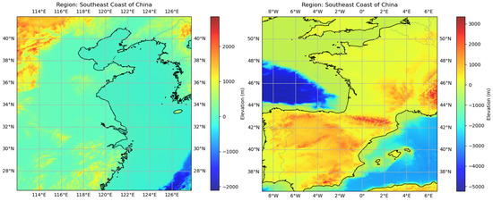
Figure 1. Topographic map of the experiment area. The horizontal coordinate represents the longitude, the vertical coordinate represents the latitude, and the colors represent the elevation.

2.2. Temporal Downscaling for Multi-Variable Meteorological Data

To solve the problem of the flexibility of existing methods being limited and it being difficult to adapt to the heterogeneity of channel information, the dynamic collaboration of flows (DCOF) is proposed in this paper to improve the representation ability of the model and adapt to the time-scaling task of multivariate meteorological data. In addition, we introduce a multi-scale warping module that uses multi-scale feature fusion representation in low-frame-rate data to enhance the performance of the network in terms of detail. Following the aforementioned description, we developed a new neural network model tailored for the temporal downscaling of meteorological data. The overall framework of the proposed network is shown in Figure 2.

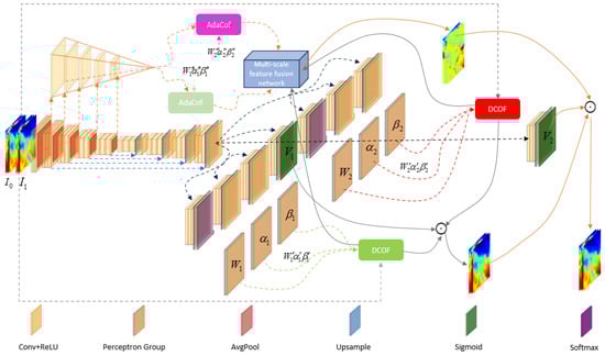
Figure 2. The overall framework of the TDNN model. The core of the TDNN mainly includes U-Net, the DCOF, and the multi-scale warping module. Its input is a composite meteorological field data frame at two adjacent time points, and its output is a synthesized composite meteorological field data frame at an intermediate time point.

Given consecutive frames of multi-variable meteorological data, $I_n$ and $I_{n+1}$, the goal of downscaling meteorological data is to synthesize intermediate time frames $I_{n+t}$ as accurately as possible; a common approach is employed by setting $t=0.5$. To accomplish this, we first identify a set or sets of warping operations $T$ that transform from $I_n$ and $I_{n+1}$ to $I_{n+t}$. For the forward and backward warping operations $T_f$ and $T_b$, we treat the combination of $I_{n+t}^1$ from $T_f\left(I_n\right)$ and $T_b\left(I_{n+1}\right)$ as components of $I_{n+t}$, and the computation process is illustrated as follows:

$$I_{n+t}^1=T_f\left(I_n\right)+T_b\left(I_{n+1}\right)$$

(1)

The warping operation in the above equation is defined as a new mechanism called the DCOF, which performs a sub-channel convolution of the input using adaptive kernel weights and bias vectors corresponding to each output position, allowing more flexibility in capturing the mapping between the input data and the desired output.

In addition, to enhance the detail rendering capability of neural networks, we create a new multi-scale feature fusion network and design a multi-scale warping module based on this, which effectively utilizes multi-scale information in the feature pyramid to generate the additional detail component $I_{n+t}$.

$$I_{n+t}^2=F_{MSF}(Cat(T_f\left(I_n\right),T_b\left(I_{n+1}\right),T_f^{\prime }\left(I\right),T_b^{\prime }\left(I\right)))$$

(2)

In this equation, $Cat(\bullet )$ denotes the concatenation operation, $T^{\prime }$ denotes the AdaCof operation, and $F_{MSF}$ denotes the multi-scale feature fusion network. Based on this, $I_{n+t}$ can be further modified as follows:

$$I_{n+t}=I_{n+t}^1+I_{n+t}^2=T_f\left(I_n\right)+T_b\left(I_{n+1}\right)+F_{MSF}(Cat(T_f\left(I_n\right),T_b\left(I_{n+1}\right),T_f^{\prime }\left(I\right),T_b^{\prime }\left(I\right)))$$

(3)

It is assumed that the input and output images are of the same size, $M\times N$ specifically. In situations with occlusion, the visibility of the target pixel differs across each input image. We introduce an occlusion map $V\in {\left[0,1\right]}^{M\times N}$ and adjust Equation (1) accordingly:

$$I_{n+t}^1=V_1\odot T_f\left(I_n\right)+(1-V_1)\odot T_b\left(I_{n+1}\right)$$

(4)

For the pixel $I_{n+t}^1(i,j)$, $V_1(i,j)=1$ signifies that the pixel is only visible in $I_n$, while $V_1(i,j)=0$ signifies that the pixel is only visible in $I_{n+1}$.

Additionally, we propose the path selection (PS) mechanism to perform the adaptive fusion of the output of the multi-scale warping module; then, Equation (3) can be modified as follows:

$$\begin{array}{ccc}{I}_{n+t}\hfill & =\hfill & V_2\odot I_{n+t}^1+(1-V_2)\odot I_{n+t}^2\hfill \\ \hfill & =\hfill & V_2\odot \left[V_1\odot T_f\left(I_n\right)+(1-V_1)\odot T_b\left(I_{n+1}\right)\right]\hfill \\ \hfill & \hfill & +(1-V_2)\odot \left[F_{MSF}(Cat(T_f\left(I_n\right),T_b\left(I_{n+1}\right),T_f^{\prime }\left(I\right),T_b^{\prime }\left(I\right)))\right]\hfill \end{array}$$

(5)

In this equation, $\odot$ represents pixel-wise multiplication; $V_2$ is a learnable mask used to combine the final results of $I_{n+t}^1$ and $I_{n+t}^2$. We anticipate that $I_{n+t}^2$ can fill in the missing contextual information in $I_{n+t}^1$.

2.3. Dynamic Collaboration of Flows

To achieve the warping of meteorological data frames from $I$ to $\widehat{I}$, we need to determine the operation $T$. To ensure that the input and output sizes remain consistent, we initially pad the input image $I$. Subsequently, we define $T$ as a conventional convolution; it can be represented in the following manner:

$$\widehat{I}(i,j)={\displaystyle \sum _{k=0}^{F-1}{\displaystyle \sum _{l=0}^{F-1}{W}_{k,l}}}I(i+k,j+l)$$

(6)

Here, $F$ represents the size of the kernel, and $W_{k,l}$ denotes the kernel weight. Deformable convolution [49] incorporates an offset vector $\Delta p_{k,l}=({\alpha }_{k,l},{\beta }_{k,l})$ into the classical convolution, as illustrated below.

$$\widehat{I}(i,j)={\displaystyle \sum _{k=0}^{F-1}{\displaystyle \sum _{l=0}^{F-1}{W}_{k,l}}}I(i+k+{\alpha }_{k,l},j+l+{\beta }_{k,l})$$

(7)

Unlike traditional deformable convolution, the shared kernel weights across various pixels are removed. Consequently, the representation of the kernel weight should be as indicated below.

$$\widehat{I}(i,j)={\displaystyle \sum _{k=0}^{F-1}{\displaystyle \sum _{l=0}^{F-1}{W}_{k,l}(i,j)}}I(i+k+{\alpha }_{k,l}(i,j),j+l+{\beta }_{k,l}(i,j))$$

(8)

However, sharing parameters across different channels in the same location still limits the degree of freedom and hinders the ability to process meteorological data with significant heterogeneity between channels. To enhance the flexibility of the DCOF, decoupling along the channel dimension $\widehat{I}(i,j)$ can be computed as shown below.

$$\widehat{I}(c,i,j)={\displaystyle \sum _{k=0}^{F-1}{\displaystyle \sum _{l=0}^{F-1}{W}_{k,l}(c,i,j)}}I(c,i+k+{\alpha }_{k,l}(c,i,j),j+l+{\beta }_{k,l}(c,i,j))$$

(9)

To allow the offset values ${\alpha }_{k,l}^c$ and ${\beta }_{k,l}^c$ to refer to any position, not limited to grid points, we employ bilinear interpolation to acquire values at non-grid locations, thus defining the value at any given position.

We broaden the starting point of the offset vector to assist the DCOF in exploring a more extensive region. Consequently, we incorporate a dilation term $d\in \left\{0,1,2\dots \right\}$, carrying out the following procedure:

$$\widehat{I}(c,i,j)={\displaystyle \sum _{k=0}^{F-1}{\displaystyle \sum _{l=0}^{F-1}{W}_{k,l}(c,i,j)}}I(i+dk+{\alpha }_{k,l}(c,i,j),j+dl+{\beta }_{k,l}(c,i,j))$$

(10)

The adjustment of parameters in the DCOF is closely related to the dynamics of atmospheric turbulence. By optimizing these parameters, we can more accurately describe multi-scale variations in different meteorological variables, such as large-scale temperature changes and small-scale pressure changes. Such adjustments not only help improve the model’s expressive power but also enhance the physical consistency between the model and actual meteorological movements.

2.4. Multi-Scale Warping Module

A common practice for interpolating frames is to calculate the target frame by mixing two warped frames with a mask. In this case, the loss of context details is inevitable due to the lack of feature space guidance. In order to improve the performance of the network in detail, we propose a multi-scale warping module. In this module, the coupling relationships of multivariable fields can be fully extracted, and detailed feature representations focused on contextual details can be generated by feeding forward- and backward-warped multi-scale feature maps into the fusion network. The structure of the multi-scale warping module (MSWM) is shown in Figure 3.

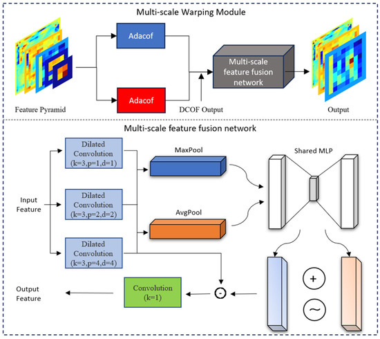
Figure 3. The overall framework of the multi-scale warping module. The module incorporates a newly designed fusion network, taking as input the feature pyramid and the output from the DCOF, with its output aimed at improving the network’s performance in detail.

Based on the multi-scale warping module, it is expected to use the multi-scale features extracted by U-Net to enhance the details of the generated data frames. Specifically, convolution operations are first used to process the output at each level in the encoder to obtain a set of multi-scale features. Then, the extracted multi-resolution features are warped based on the AdaCof operation to capture motion information in the feature space. Finally, based on the multi-scale feature fusion network, the multi-scale feature map containing displacement information is processed by the adaptive weighting of the channel, and the data frame with the details is generated by making full use of the cross-channel interaction information. The multi-scale feature fusion method has played a crucial role in this study, especially in capturing meteorological phenomena at different spatial scales. In terms of physical mechanisms, multi-scale feature fusion can effectively simulate energy transfer and information exchange between different scales. For example, the interaction between humidity and temperature fields has different physical characteristics at different spatial scales, and by integrating this information, the model can better describe complex phenomena in the atmosphere.

2.5. Evaluation Methods

The mean absolute error (MAE) measures the average deviation between predicted and actual values by computing the mean of all absolute errors, providing an intuitive representation of overall error magnitude. In contrast, the root mean square error (RMSE) is derived by taking the square root of the mean of squared errors, making it more sensitive to larger deviations and thus a more responsive metric for error assessment. Both the MAE and RMSE are widely used to quantify pixel-level errors in reconstructed fields, with their respective formulas as follows:

$$RMSE=\sqrt{{\displaystyle \frac{1}{N}}{\displaystyle \sum _{i=1}^N{(G_i-O_i)}^2}}$$

(11)

$$MAE={\displaystyle \frac{1}{N}}{\displaystyle \sum _{i=1}^N|G_i-O_i|}$$

(12)

In the formulas, $G_i$ stands for the ground-truth data, $O_i$ represents the reconstructed field, and $N$ is the total number of data points. In this paper, the ground-truth data refer to the real reference data used to evaluate the results of the model.

In correlation analysis, directly comparing weather forecasts with actual observations or analysis data may lead to misleadingly high correlations due to the influence of seasonal variations. Therefore, the standard approach is to first remove the climate mean from both forecast and observation data to mitigate the impact of seasonal cycles. Then, the anomaly correlation coefficient (ACC) is used to assess the consistency between the anomalies of the forecast and observation fields. The calculation formula is typically expressed as follows:

$$ACC={\displaystyle \frac{{\displaystyle {\sum }_{i,j,k}{f}_{i,j,k}^{\prime }{t}_{i,j,k}^{\prime }}}{\sqrt{{\displaystyle {\sum }_{i,j,k}{f}_{i,j,k}^{\prime 2}{\displaystyle {\sum }_{i,j,k}{t}_{i,j,k}^{\prime 2}}}}}}$$

(13)

where the superscript ′ indicates the difference from climatology, $f$ stands for the forecast value, and $t$ stands for the observed value or label value.

The peak signal-to-noise ratio (PSNR) is a key metric for assessing the ratio between the peak signal energy and the average noise energy, commonly used to evaluate data frame quality. However, since the PSNR is directly computed based on error magnitude, it may not accurately capture the perceptual characteristics of the human visual system, potentially leading to discrepancies between the evaluation results and actual visual perception. To provide a more comprehensive assessment of model output quality, this study incorporates the structural similarity index (SSIM), which better aligns with the HVS by capturing the structural features of images. Accordingly, both the PSNR and SSIM are employed to evaluate the spatial distribution of the model’s downscaling results, with their respective formulas expressed as follows:

$$PSNR=10\lg {\displaystyle \frac{I_{max}^2}{MSE}}$$

(14)

$$SSIM={\displaystyle \frac{(2{\mu }_G{\mu }_0+c_1)(2{\sigma }_{GO}+c_2)}{({\mu }_G^2+{\mu }_O^2+c_1)({\sigma }_G^2+{\sigma }_O^2+c_2)}}$$

(15)

$I_{max}$ refers to the bit depth of the data. For natural images with the uint8 data type, the value is 255. When calculating the PSNR and SSIM for meteorological fields, we transform the data range to (0, 255), allowing it to be calculated as 255.

3. Results

3.1. Ablation Study

To evaluate the effectiveness of our proposed method, we performed ablation studies on the DCOF, multi-scale warping module (MSWM), and path selection (PS). The experiment was conducted uniformly on Ubuntu computing platforms equipped with XEON 6226 R and RTX 3090, using Cuda version 11.6 and Cudnn version 8.4.1; the results are shown in Table 1. In this study, TDNN-MSWM refers to the removal of the multi-resolution warping module, and TDNN-PS represents the ablation of path selection in the TDNN. The results demonstrate that both the multi-scale warping module and path selection contribute positively to model performance, with the MSWM playing a particularly crucial role in reducing errors and enhancing detail reconstruction. In the SP task, the removal of the MSWM led to an MAE increase of 1.36, an RMSE increase of 2.48, and a PSNR drop of 0.78 dB, while in the composite task, removing the MSWM resulted in an MAE increase of 0.46, an RMSE increase of 1.43, and a PSNR drop of 0.42 dB. This may be due to the difficulty in obtaining multi-scale context information and cross-channel coupling information after MSWM ablation. This phenomenon directly indicates that the MSWM plays an important role in global information compensation and detail refinement and verifies the importance of modeling multi-field coupling relationships to improve downscaling effects. In contrast, PS primarily affects detail fusion, with its removal causing relatively smaller increases in the MAE and RMSE but still leading to a 0.5 dB decrease in the PSNR for the T2M task, demonstrating its effectiveness in pixel-level optimization. Overall, the MSWM is more critical in ensuring the model’s robustness and fidelity across different tasks, while the PS mechanism further optimizes local details. Together, they complement each other to enhance the overall model performance.

Table 1. Ablation experiment results.

Project		MAE ↓	RMSE ↓	ACC ↑	PSNR ↑	SSIM ↑
T2M	TDNN	0.158	0.280	0.99951	50.507	0.9937
	TDNN-PS	0.170	0.296	0.99945	50.007	0.9926
	TDNN-MSWM	0.168	0.295	0.99945	50.049	0.9925
SP	TDNN	20.064	26.479	0.99948	60.034	0.9983
	TDNN-PS	20.339	26.643	0.99947	59.981	0.9982
	TDNN-MSWM	21.425	28.956	0.99937	59.258	0.9982
SH1000	TDNN	0.071	0.128	0.99971	49.407	0.9946
	TDNN-PS	0.074	0.134	0.99969	49.021	0.9944
	TDNN-MSWM	0.073	0.133	0.99969	49.052	0.9944
Composite	TDNN	6.764	15.289	0.99947	51.477	0.9955
	TDNN-PS	6.861	15.384	0.99946	51.058	0.9951
	TDNN-MSWM	7.222	16.719	0.99937	51.058	0.9951

Note: The best results have been bolded. The up and down arrows indicate that the larger and smaller numerical results are optimal, respectively.

It should be pointed out that compared with the RMSE, MAE, and ACC, the performance changes in the model after the ablation of some modules are not obvious in the ACC and SSIM metrics. This may be because the ACC and SSIM are more sensitive to the distribution bias of the model output, while the TDNN can reconstruct the data distribution of intermediate frames well after ablating the PS and MSWM. This phenomenon is very common in the field of super-resolution [50]. Although some scholars may selectively use these indicators in experiments to avoid misunderstandings [51], we believe that disclosing these data contributes to a more comprehensive assessment of performance changes. Although the displayed error differences are relatively small, we believe that these differences are still noteworthy in the context of model optimization and module analysis. The main innovation of this article lies in the DCOF, PS, and MSWM. After ablating the PS and MSWM, the model still retains the main structure based on the DCOF, and the small performance change may be due to the performance advantage of the model mainly coming from the DCOF. However, this does not mean that the PS and MSWM are not important enough. Each module has a different role in the model, and even small changes may have an impact on the performance of the model in specific contexts. Therefore, we believe that this small difference reflects the sensitivity of the model under different configurations and can provide valuable references for model improvement.

3.2. Performance Analysis

We systematically evaluated the performance of our proposed model by comparing it against state-of-the-art interpolation algorithms and deep neural network methods. Metrics such as the MAE, RMSE, ACC, PSNR, and SSIM were employed across various meteorological fields, including T2M, SP, and SH1000, as summarized in Table 2, Table 3 and Table 4. Overall, our model consistently delivered superior results across all downscaling tasks, achieving the lowest RMSE and the highest ACC, PSNR, and SSIM in every field. In particular, our model significantly outperformed the AdaCof method in every temporal downscaling scenario, a result attributable to its effective multi-scale feature integration and advanced temporal alignment strategies. Ablation studies further demonstrated that even without certain architectural enhancements, our model still exhibited a lower MAE than AdaCof in both the T2M and SH1000, highlighting its robustness in handling complex meteorological variations. Moreover, our method substantially outperformed classical interpolation techniques. For example, in the SP field, our model reduced the MAE and RMSE by 50.44% and 53.73%, respectively, compared to Cubic interpolation, and by 43.05% and 51.09% when compared to deep learning models such as EDSC. The improvements in the ACC, PSNR, and SSIM were also substantial, reaffirming its ability to preserve structural and statistical properties in downscaled outputs. Interestingly, despite the general advantage of deep learning models in expressive power and nonlinear fitting, certain methods like the RRIN and VFIformer performed worse than interpolation-based methods such as Cubic. This is likely due to their original design for video frame interpolation, which is less suited for capturing the intricate correlations and heterogeneity inherent in multivariate meteorological data. Compared to AdaCof, our method can achieve cross-channel heterogeneous information extraction, greater flexibility, and reduced contextual detail loss, thereby outperforming AdaCof across all metrics and meteorological fields. Notably, in the SH1000 field, our model showed the largest improvement over AdaCof, with gains of 22.83%, 25.15%, and 5.36% in the MAE, RMSE, and PSNR, respectively. These findings underscore the superior performance of our model for multivariate meteorological downscaling and affirm the effectiveness of our architectural innovations.

Table 2. Performance evaluation results of each model in time downscaling of T2M field.

Model	MAE (k) ↓	RMSE (k) ↓	ACC ↑	PSNR ↑	SSIM ↑
Cubic	0.850	1.652	0.9832	35.082	0.9534
CAIN [52]	1.027	1.441	0.9938	36.272	0.9195
EDSC [49]	0.198	0.319	0.9994	49.356	0.9925
AdaCof [40]	0.178	0.299	0.9994	49.921	0.9928
FILM [53]	0.748	1.198	0.9910	37.875	0.9389
FLAVR [54]	0.181	0.294	0.9994	50.084	0.9926
SepConv++ [55]	0.422	0.735	0.9966	42.117	0.9867
RRIN [56]	3.507	6.671	0.7311	22.960	0.7376
SepConv [38]	0.252	0.387	0.9991	47.700	0.9919
DVF [57]	0.318	0.521	0.9983	45.111	0.9900
VFIformer [58]	5.573	8.577	0.4605	20.777	0.5378
Zooming Slow-Mo [59]	0.189	0.303	0.9994	49.811	0.9932
Ours	0.158	0.280	0.9995	50.507	0.9937

Note: The best results have been bolded. The up and down arrows indicate that the larger and smaller numerical results are optimal, respectively.

Table 3. Performance evaluation results of each model in time downscaling of SP field.

Model	MAE (pa) ↓	RMSE (pa) ↓	ACC ↑	PSNR ↑	SSIM ↑
Cubic	40.488	57.226	0.9975	53.341	0.9955
CAIN [52]	209.812	271.595	0.9509	39.814	0.9078
EDSC [49]	35.233	54.136	0.9978	53.823	0.9972
AdaCof [40]	20.777	27.39	0.9994	59.741	0.9983
FILM [53]	441.655	792.393	0.6638	30.514	0.9225
FLAVR [54]	28.217	37.046	0.9991	57.118	0.9971
SepConv++ [55]	20.942	27.787	0.9994	59.616	0.9982
RRIN [56]	1630.097	3923.896	0.1795	16.618	0.8158
SepConv [38]	52.606	83.071	0.9949	50.104	0.9955
DVF [57]	32.957	51.519	0.9980	54.253	0.9981
VFIformer [58]	2695.569	4387.114	0.0363	15.649	0.5266
Zooming Slow-Mo [59]	32.802	43.036	0.9988	55.816	0.9974
Ours	20.064	26.479	0.9995	60.034	0.9983

Note: The best results have been bolded. The up and down arrows indicate that the larger and smaller numerical results are optimal, respectively.

Table 4. Performance evaluation results of each model in time downscaling of SH1000 field.

Model	MAE ↓ (g/kg)	RMSE ↓ (g/kg)	ACC ↑	PSNR ↑	SSIM ↑
Cubic	0.216	0.391	0.9973	39.713	0.9690
CAIN [52]	0.741	0.980	0.9928	31.725	0.8884
EDSC [49]	0.087	0.148	0.9996	48.156	0.9935
AdaCof [40]	0.092	0.171	0.9995	46.892	0.9924
FILM [53]	0.449	0.690	0.9921	34.766	0.9223
FLAVR [54]	0.084	0.138	0.9996	48.746	0.9934
SepConv++ [55]	0.084	0.150	0.9996	48.029	0.9934
RRIN [56]	2.762	3.729	0.7710	20.115	0.6016
SepConv [38]	0.107	0.171	0.9995	46.914	0.9916
DVF [57]	0.094	0.168	0.9995	47.021	0.9924
VFIformer [58]	3.754	4.676	0.5414	18.150	0.4398
Zooming Slow-Mo [59]	0.080	0.129	0.9996	49.345	0.9945
Ours	0.071	0.128	0.9997	49.407	0.9946

Note: The best results have been bolded. The up and down arrows indicate that the larger and smaller numerical results are optimal, respectively.

3.3. Robustness Analysis

Ensuring stable generation errors over time, a property referred to as “temporal robustness”, is essential in the temporal downscaling of meteorological data. To evaluate this, we conducted a comparative analysis of different models applied to a composite meteorological field, as illustrated in Figure 4. Note that due to the nature of time downscaling, the error values corresponding to even moments in the figure have no practical significance. Our study assessed the variation in errors across different time points using key evaluation metrics, including the MAE, RMSE, ACC, and SSIM. Deep learning-based models generally show strong time robustness, but their error fluctuations differ over time. Among the models evaluated, our approach achieves significant performance improvements. Compared to the baseline methods, our model significantly reduced the MAE and RMSE while consistently attaining higher ACC and SSIM scores. The fluctuations in the MAE and RMSE remain minimal, indicating superior stability. Specifically, the ACC fluctuation range is nearly negligible, reflecting strong consistency over time. These findings suggest that our model not only achieves higher overall accuracy but also ensures better consistency across different time points, making it highly effective for the temporal downscaling of meteorological data.

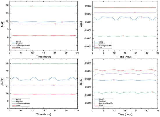
Figure 4. The generation error of various models in the composite meteorological field as time changes. In each subplot, the x-axis shows the lead time, and the y-axis represents different evaluation metrics. The smaller the MAE and RMSE values, the better the performance. The higher the values of the ACC and SSIM, the better the performance. The optimal result in each curve is shown by the red circle.

It is well known that machine learning assumes that the samples are independent and equally distributed. In this hypothesis, replacing the existing training data with statistically homogeneous data theoretically has no significant impact on the testing effect of the model. However, even if the data are statistically homogeneous, there may still be random errors and uncertainties between different data samples that may affect the optimization process of the model. Therefore, there may be some fluctuations in the model’s performance. To evaluate the effect of changes in the training dataset on the error, we retrained and validated the model using data from different years. In the new experiment, we trained using data from 2018 and 2019, and the test data remained the same. The experimental results are shown in Table 5 and Table 6; TDNN-1 represents the model trained with the default data, and TDNN-2 represents the model trained with the new data from 2018 to 2019. The results in Table 5 show that although the error changes slightly after the replacement of training data, the overall trend of error changes after the ablation of different modules does not change significantly. This may be because the error difference of the model is often determined by the expressiveness of the model and the change law of the meteorological variables. Even with different datasets, the relative trend of the error and the performance of the model sensitivity still have a certain regularity. In addition, although the error value fluctuates after the training data change, the change trend of the error difference is generally consistent. This shows that the module function and model performance have certain stability under similar meteorological phenomena. The experimental results in Table 6 show that the error fluctuation caused by training data replacement does not exceed 3.91% of the original error. Due to the small error of the SH1000, a slight fluctuation may produce a large percentage deviation, but it should be noted that the error at this time is reduced compared to the original error, and the fluctuation is still small and will not affect the use of the model. On the other hand, compared with the original error, the average fluctuation is only about 0.74%, which indicates that the proposed model has good robustness and reliability.

Table 5. Results of ablation experiments on new training data.

Project		MAE ↓	RMSE ↓	ACC ↑	PSNR ↑	SSIM ↑
T2M	TDNN	0.158	0.279	0.99952	50.545	0.9940
	TDNN-PS	0.169	0.291	0.99947	50.170	0.9933
	TDNN-MSWM	0.172	0.298	0.99944	49.951	0.9925
SP	TDNN	19.811	26.023	0.99950	60.208	0.9983
	TDNN-PS	22.288	29.860	0.99934	59.063	0.9982
	TDNN-MSWM	22.806	30.814	0.99929	58.755	0.9982
SH1000	TDNN	0.069	0.123	0.99975	49.725	0.9951
	TDNN-PS	0.074	0.134	0.99969	49.015	0.9944
	TDNN-MSWM	0.073	0.129	0.99971	49.329	0.9948
Composite	TDNN	6.679	15.025	0.99949	51.667	0.9958
	TDNN-PS	7.510	17.241	0.99933	51.228	0.9954
	TDNN-MSWM	7.684	17.792	0.99929	50.977	0.9951

Note: The best results have been bolded. The up and down arrows indicate that the larger and smaller numerical results are optimal, respectively.

Table 6. Performance of the model when using different training data.

Project		MAE ↓	RMSE ↓	ACC ↑	PSNR ↑	SSIM ↑
T2M	TDNN-1	0.158	0.280	0.9995	50.507	0.9937
	TDNN-2	0.158	0.279	0.9995	50.545	0.9940
	Deviation (%)	0.00	−0.36	0.00	0.08	0.03
SP	TDNN-1	20.064	26.479	0.9995	60.034	0.9983
	TDNN-2	19.811	26.023	0.9995	60.208	0.9983
	Deviation (%)	−1.26	−1.72	0.00	0.29	0.00
SH1000	TDNN-1	0.071	0.128	0.9997	49.407	0.9946
	TDNN-2	0.069	0.123	0.9998	49.725	0.9951
	Deviation (%)	−2.82	−3.91	0.01	0.64	0.05

Note: The up and down arrows indicate that the larger and smaller numerical results are optimal, respectively.

3.4. Visual Analysis

Figure 5 illustrates the differences between the time downscaling results obtained by different methods and the ground truth. The study area encompasses a complex meteorological environment, where the analyzed variables are significantly influenced by the terrain, exhibiting rich spatiotemporal variations. Traditional interpolation methods, such as Cubic, tend to produce blurry and inaccurate results, failing to effectively capture high-frequency details. In contrast, our proposed method integrates the dynamic collaboration of flows, a multi-scale warping module, and an adaptive path selection strategy, enabling the generation of clearer and more realistic results. Compared to advanced models such as SepConv, EDSC, and AdaCof, our method demonstrates superior spatial consistency and accuracy, better preserving fine-grained meteorological structures. Notably, although EDSC employs deformable convolutions for feature extraction, it still exhibits limitations in reconstructing fine-scale details. Similarly, AdaCof performs well in certain regions but lacks adaptability across different meteorological variables. Overall, these results highlight the superior performance and robustness of our model in high-precision meteorological data time downscaling tasks.

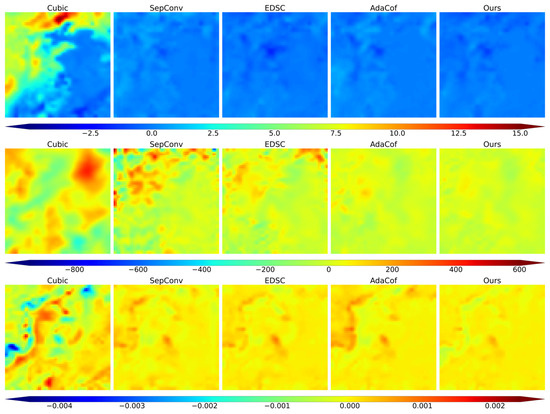
Figure 5. Visualization of difference field between model output and ground truth. The first through third rows show the T2M difference field (K), SP difference field (Pa), and SH1000 difference field (Kg/Kg), respectively. In these images, points with values closer to 0 indicate a smaller discrepancy from the ground truth.

3.5. Scalability Exploration

To explore the scalability, the performance of the model was tested in the 6 h interval meteorological field. Table 7 evaluates the performance in the task, using the MAE, RMSE, and ACC as evaluation metrics. The results indicate that deep learning methods generally outperform traditional interpolation methods (such as Cubic), though there are still significant differences in performance among different models. For all evaluation metrics across the three variables, the T2M (temperature), SP (surface pressure), and SH1000 (specific humidity), our method achieves the best results in the MAE, RMSE, and ACC, demonstrating superior time downscaling capabilities compared to other approaches. Specifically, compared with other deep learning methods, our approach achieves a significant reduction in the MAE and RMSE, while the ACC values reach 0.9973, 0.9983, and 0.9977, indicating higher prediction accuracy and data consistency. For instance, in the SP (surface pressure) prediction task, our method reduces the MAE and RMSE by 5.18% and 2.93%, respectively, compared to FLAVR, and by 62.06% and 63.67%, respectively, compared to EDSC. These results indicate that, in the face of downscaling tasks with varying time intervals, our method not only significantly outperforms existing models in overall accuracy but also exhibits strong scalability.

Table 7. Performance evaluation of models in the time downscaling of 6 h interval field.

Model	T2M			SP			SH1000
	MAE ↓ (k)	RMSE ↓ (k)	ACC ↑	MAE ↓ (pa)	RMSE ↓ (pa)	ACC ↑	MAE ↓ (g/kg)	RMSE ↓ (g/kg)	ACC ↑
Cubic	2.022	3.542	0.9289	132.463	194.027	0.9740	0.645	1.103	0.9794
CAIN [52]	1.200	1.898	0.9929	175.684	226.030	0.9736	0.762	1.118	0.9932
EDSC [49]	0.516	0.756	0.9964	93.095	131.280	0.9872	0.274	0.407	0.9971
AdaCof [40]	0.493	0.771	0.9963	48.026	69.093	0.9965	0.267	0.406	0.9971
FILM [53]	0.963	1.390	0.9880	292.344	486.038	0.8503	0.420	0.594	0.9938
FLAVR [54]	0.432	0.661	0.9972	37.254	49.135	0.9982	0.248	0.367	0.9976
SepConv++ [55]	0.917	1.371	0.9882	62.429	79.682	0.9952	0.289	0.441	0.9966
SepConv [38]	0.790	1.150	0.9917	156.555	240.836	0.9585	0.332	0.485	0.9958
DVF [57]	0.646	0.979	0.9940	74.463	100.861	0.9924	0.279	0.422	0.9969
Ours	0.426	0.661	0.9973	35.324	47.694	0.9983	0.240	0.365	0.9977

Note: The best results have been bolded. The up and down arrows indicate that the larger and smaller numerical results are optimal, respectively.

To explore the performance of the model in the discontinuous spatiotemporal field, we selected total precipitation (TP) as a new experimental variable. Given the stable performance of EDSC and SepConv, we included them as representative deep learning models for visual comparison. Figure 6 visualizes the TP fields from the ERA5 dataset and the outputs of various models. In the visualization results, the ERA5 dataset serves as the ground truth for precipitation distribution. However, compared to ERA5, existing methods exhibit noticeable issues at different times, such as the blurring of precipitation regions, distortion of boundaries, and loss of details. Particularly in marked regions, the CAIN and SepConv fail to effectively preserve the structural integrity of precipitation patterns. In particular, the CAIN produces a large number of false details in some areas. In contrast, our method accurately captures the temporal evolution of precipitation, producing results that closely resemble the ERA5 data. This indicates that our approach maintains better temporal consistency and structural fidelity. Table 8 shows the results of the quantitative evaluation, in which our approach achieved the best performance across all metrics. Specifically, it achieves the lowest error values, demonstrating superior prediction accuracy and reduced errors compared to other methods. Additionally, it attains the highest values for the PSNR and SSIM, indicating that our method best preserves the original data quality and structural information. Furthermore, our approach achieves the highest ACC among all tested methods, further verifying its stability and reliability. Overall, our method effectively reduces prediction errors and can still effectively restore the spatial structure and temporal evolution of variables in the time downscaling task of discontinuous fields represented by total precipitation. This further validates the scalability of the proposed method and makes it a more reliable solution for high-precision time downscaling.

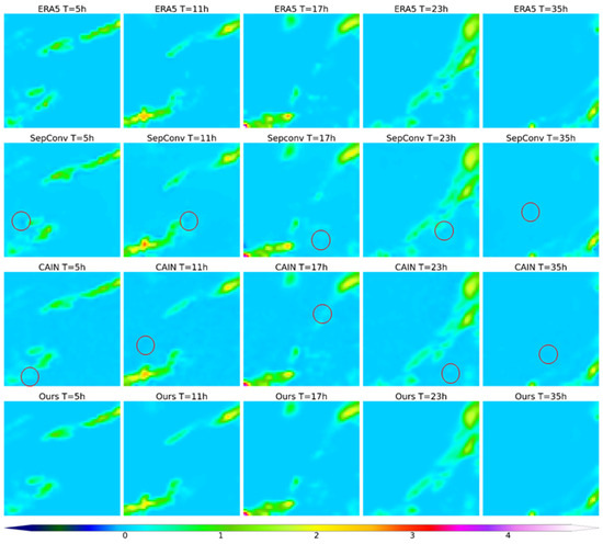
Figure 6. Visual comparison of total precipitation field between model output and ground truth. Rows 1 to 4 are the ERA5 data and the output of the SepConv, CAIN, and TDNN models, respectively. The circles indicate potentially critical areas to focus on. The unit is mm.

Table 8. Performance evaluation of models in the time downscaling of 6 h interval TP field.

Model	MAE ↓ (mm)	RMSE ↓ (mm)	ACC ↑	PSNR ↑	SSIM ↑
CAIN [52]	0.068	0.230	0.9313	51.373	0.8869
EDSC [49]	0.067	0.227	0.9329	51.476	0.9447
AdaCof [40]	0.047	0.212	0.9421	52.095	0.9478
FILM [53]	0.058	0.236	0.9273	51.131	0.9411
FLAVR [54]	0.051	0.214	0.9407	51.974	0.9452
SepConv++ [55]	0.052	0.231	0.9303	51.327	0.9434
SepConv [38]	0.078	0.252	0.9188	50.568	0.9328
Ours	0.046	0.211	0.9426	52.131	0.9492

Note: The best results have been bolded. The up and down arrows indicate that the larger and smaller numerical results are optimal, respectively.

3.6. Transferability Analysis

We used the trained model to downscale weather fields at 6 h intervals in the new region to assess their transferability, and the results are shown in Figure 7. The experimental results show that our method has superior transferability in time-scaling tasks in new regions. Compared with the FILM, FLAVR, SepConv, and Zooming Slow-Mo methods, the error of our method is lower for different meteorological variables (T2M, SP, SH1000), especially the SP variable, for which the error reduction is most significant. In addition, from the perspective of error distribution, our method presents a more uniform error distribution in space and avoids obvious high-error regions, indicating that it has stronger adaptability in different regions and different meteorological conditions.

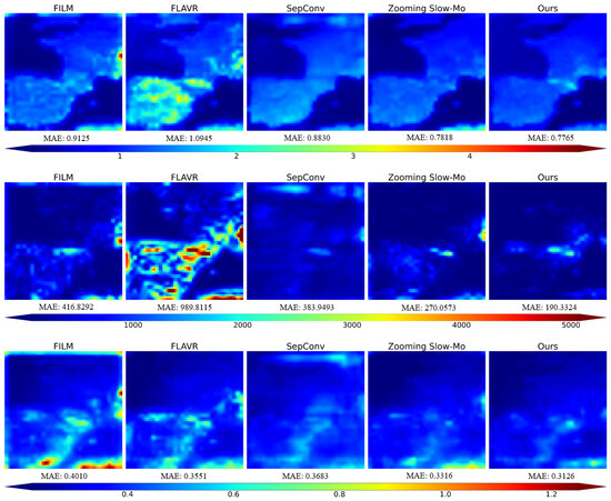
Figure 7. Visualization of difference field between model output and ground truth. Rows 1 to 3 represent T2M, SP, and SH1000, respectively.

Further combined with the test results of each model in the training area, our method achieved optimal performance for the T2M, SP and SH1000 variables in the training area, with the smallest MAE and RMSE and the highest ACC, which fully proved its excellent fitting ability. At the same time, in the new region, our method still maintains the lowest error and shows a more uniform error distribution, indicating that its generalization ability is strong and it can adapt to different spatial environments. In contrast, although methods such as FLAVR and FILM perform well for the partial variables of the training region, the errors in the new region increase significantly, indicating that their transferability is weak. In general, our method not only performs best in the training area but also remains stable in the unseen area, showing strong cross-regional applicability and transferability.

4. Discussion

4.1. Interpretation of Results

Our study demonstrates the effectiveness of the proposed model in improving the temporal downscaling performance for meteorological data. The ablation study results indicate that both the multi-scale warping module (MSWM) and path selection (PS) significantly contribute to performance enhancement. Specifically, the MSWM plays a crucial role in reducing errors and preserving fine-grained details, as evidenced by the substantial increases in the MAE and RMSE upon its removal. Meanwhile, PS facilitates pixel-level optimization, leading to notable PSNR improvements. These findings confirm the importance of modeling multi-field coupling relationships for accurate downscaling.

The performance comparison further reinforces the superiority of our model over state-of-the-art interpolation and deep learning approaches. Our model consistently achieves the lowest MAE and RMSE and the highest ACC, PSNR, and SSIM across various meteorological fields, underscoring its robustness and adaptability. Notably, even without certain architectural enhancements, our model still surpasses AdaCof in the MAE for both the T2M and SH1000, demonstrating its resilience against complex meteorological variations.

4.2. Comparison with Existing Methods

Compared with classical interpolation techniques, our method exhibits significant improvements. For instance, in the SP field, it achieves a 50.44% and 53.73% reduction in the MAE and RMSE, respectively, over Cubic interpolation. Additionally, compared to deep learning models such as EDSC, our model maintains superior performance in structural preservation and detail refinement. While some deep learning models, such as the RRIN and VFIformer, are difficult to adapt to multivariate meteorological data due to their design objectives and the inherent limitations of network structure, our method effectively extracts cross-channel heterogeneous information, resulting in improved accuracy and lower contextual detail loss.

Moreover, the robustness analysis indicates that our model maintains stable error margins over time. This is a crucial advantage in temporal downscaling applications, as fluctuations in prediction accuracy can compromise forecasting reliability. The visual analysis corroborates these findings, revealing that our model preserves spatial consistency and fine-grained meteorological structures better than competing methods, including SepConv, EDSC, and AdaCof.

4.3. Limitations and Future Work

Despite its strong performance, our model has certain limitations. On the one hand, while our approach shows superior versatility across different meteorological variables, its effectiveness under extreme weather conditions or where data are missing has not been widely validated. Additional trials with rare and high-impact weather events, as well as missing data scenarios, are needed to assess its adaptability and reliability. On the other hand, while our model achieves remarkable downscaling accuracy, the potential integration of physical constraints or domain-specific knowledge into the learning process remains an open question. Hybrid approaches combining deep learning with physical models may further improve interpretability and reliability in operational forecasting applications.

In addition, although the TDNN model proposed in this paper demonstrates excellent performance, it contains several complex components (such as the DCOF module and the multi-scale warping module), which may increase the computational cost of model training and inference. According to our statistics, the number of parameters in the proposed model is approximately 45.94 million, which is significantly lower than that of comparative models such as the CAIN (approximately 49.78 million). The inference time per data frame is only 27.87 ms, slightly lower than the 29.17 ms required by Sepconv++ and significantly lower than the 32.24 ms required by Zooming Slow-Mo. Nevertheless, we believe that through techniques such as model compression and lightweight design, it is still possible to significantly improve the model’s computational efficiency while maintaining its performance, thereby enhancing its practicality and promoting the widespread use of the proposed method in small-scale meteorological monitoring stations or mobile-device-based applications.

5. Conclusions

In remote sensing applications, time downscaling to accurately capture temporal dynamics is very important to improve the resolution and continuity of meteorological data. At the same time, learning the mapping relationship between low-resolution and high-resolution data and effectively downscaling historical meteorological data to obtain long time series and high-frame-rate information are key guarantees for the accurate operation of models in various fields. To address this, we propose the TDNN, a deep neural network designed for the temporal downscaling of multivariate meteorological data, incorporating a dynamic collaboration of flows for greater flexibility. To mitigate the contextual information loss inherent in raw pixel-based methods, we introduce a multi-resolution warping module.

The TDNN uses a U-Net framework and integrates the DCOF, a multi-scale warping module, and a path selection mechanism to optimize information extraction and integration. Ablation experiments show that the DCOF has stronger adaptability to spatiotemporal heterogeneity, the multi-scale warping module can significantly enhance the generated details, and the path selection mechanism can optimize data fusion, which together improve the overall performance of the model. Compared to traditional interpolation methods (such as Cubic) and deep learning methods (such as FLAVR), the TDNN performs well in terms of performance, time robustness, task scalability, and transferability and achieves optimal results across all meteorological variables. These results highlight the key role of high-degree-of-freedom dynamic modeling in complex meteorological dynamics and highlight the importance of optimizing the context details in the feature space in the time downscaling of meteorological data, suggesting the great application potential of the TDNN in remote sensing data and meteorological data enhancement.

References

- Li, J.; Zhao, J.; Lu, Z. A typical meteorological day database of solar terms for simplified simulation of outdoor thermal environment on a long-term. Urban Clim. 2024, 57, 102117. [Google Scholar] [CrossRef]
- Ding, X.; Zhao, Y.; Fan, Y.; Li, Y.; Ge, J. Machine learning-assisted mapping of city-scale air temperature: Using sparse meteorological data for urban climate modeling and adaptation. Build. Environ. 2023, 234, 110211. [Google Scholar] [CrossRef]
- Mohanty, A.; Sahoo, B.; Kale, R.V. A hybrid model enhancing streamflow forecasts in paddy land use-dominated catchments with numerical weather prediction model-based meteorological forcings. J. Hydrol. 2024, 635, 131225. [Google Scholar] [CrossRef]
- Long, J.; Xu, C.; Wang, Y.; Zhang, J. From meteorological to agricultural drought: Propagation time and influencing factors over diverse underlying surfaces based on CNN-LSTM model. Ecol. Inform. 2024, 82, 102681. [Google Scholar] [CrossRef]
- Jeong, D.I.; St-Hilaire, A.; Ouarda, T.B.M.J.; Gachon, P. A multi-site statistical downscaling model for daily precipitation using global scale GCM precipitation outputs. Int. J. Climatol. 2013, 33, 2431–2447. [Google Scholar] [CrossRef]
- Ma, M.; Tang, J.; Ou, T.; Zhou, P. High-resolution climate projection over the Tibetan Plateau using WRF forced by bias-corrected CESM. Atmos. Res. 2023, 286, 106670. [Google Scholar] [CrossRef]
- Zhao, G.; Li, D.; Camus, P.; Zhang, X.; Qi, J.; Yin, B. Weather-type statistical downscaling for ocean wave climate in the Chinese marginal seas. Ocean Model. 2024, 187, 102297. [Google Scholar] [CrossRef]
- Richardson, C.W. Stochastic simulation of daily precipitation, temperature, and solar radiation. Water Resour. Res. 1981, 17, 182–190. [Google Scholar] [CrossRef]
- Richardson, C.W.; Wright, D.A. WGEN: A Model for Generating Daily Weather Variables; United States Department of Agriculture: Washington, DC, USA, 1984.
- Semenov, M. Simulation of extreme weather events by a stochastic weather generator. Clim. Res. 2008, 35, 203–212. [Google Scholar] [CrossRef]
- Li, S.; Xu, C.; Su, M.; Lu, W.; Chen, Q.; Huang, Q.; Teng, Y. Downscaling of environmental indicators: A review. Sci. Total Environ. 2024, 916, 170251. [Google Scholar] [CrossRef]
- Vandal, T.; Kodra, E.; Ganguly, S.; Michaelis, A.; Nemani, R.; Ganguly, A.R. DeepSD: Generating high resolution climate change projections through single image super-resolution. In Proceedings of the 23rd ACM Sigkdd International Conference on Knowledge Discovery and Data Mining, Halifax, NS, Canada, 13–17 August 2017; ACM: New York, NY, USA, 2017. [Google Scholar]
- Rodrigues, E.R.; Oliveira, I.; Cunha, R.; Netto, M. DeepDownscale: A deep learning strategy for high-resolution weather forecast. In Proceedings of the 2018 IEEE 14th International Conference on e-Science (e-Science), Amsterdam, The Netherlands, 29 October–1 November 2018; pp. 415–422. [Google Scholar]
- Pan, B.; Hsu, K.; AghaKouchak, A.; Sorooshian, S. Improving precipitation estimation using convolutional neural network. Water Resour. Res. 2019, 55, 2301–2321. [Google Scholar] [CrossRef]
- Yu, M.; Liu, Q. Deep learning-based downscaling of tropospheric nitrogen dioxide using ground-level and satellite observations. Sci. Total Environ. 2021, 773, 145145. [Google Scholar] [CrossRef]
- Qian, X.; Qi, H.; Shang, S.; Wan, H.; Rahman, K.U.; Wang, R. Deep learning-based near-real-time monitoring of autumn irrigation extent at sub-pixel scale in a large irrigation district. Agric. Water Manag. 2023, 284, 108335. [Google Scholar] [CrossRef]
- Sahour, H.; Sultan, M.; Vazifedan, M.; Abdelmohsen, K.; Karki, S.; Yellich, J.A.; Gebremichael, E.; Alshehri, F.; Elbayoumi, T.M. Statistical applications to downscale GRACE-derived terrestrial water storage data and to fill temporal Gaps. Remote Sens. 2020, 12, 533. [Google Scholar] [CrossRef]
- Lu, M.; Jin, C.; Yu, M.; Zhang, Q.; Liu, H.; Huang, Z.; Dong, T. MCGLN: A multimodal ConvLSTM-GAN framework for lightning nowcasting utilizing multi-source spatiotemporal data. Atmos. Res. 2024, 297, 107093. [Google Scholar] [CrossRef]
- Uz, M.; Akyilmaz, O.; Shum, C. Deep learning-aided temporal downscaling of GRACE-derived terrestrial water storage anomalies across the Contiguous United States. J. Hydrol. 2024, 645, 132194. [Google Scholar] [CrossRef]
- Cheng, J. Research on Meteorological Forecasting System Based on Deep Learning Super-Resolution. Master’s Thesis, Wuhan University, Wuhan, China, 2021. [Google Scholar]
- Tian, H.; Wang, P.; Tansey, K.; Wang, J.; Quan, W.; Liu, J. Attention mechanism-based deep learning approach for wheat yield estimation and uncertainty analysis from remotely sensed variables. Agric. For. Meteorol. 2024, 356, 110183. [Google Scholar] [CrossRef]
- Xiao, Y.; Wang, Y.; Yuan, Q.; He, J.; Zhang, L. Generating a long-term (2003–2020) hourly 0.25° global PM2.5 dataset via spatiotemporal downscaling of CAMS with deep learning (DeepCAMS). Sci. Total Environ. 2022, 848, 157747. [Google Scholar] [CrossRef]
- Najibi, N.; Perez, A.J.; Arnold, W.; Schwarz, A.; Maendly, R.; Steinschneider, S. A statewide, weather-regime based stochastic weather generator for process-based bottom-up climate risk assessments in California—Part I: Model evaluation. Clim. Serv. 2024, 34, 100489. [Google Scholar] [CrossRef]
- Busch, U.; Heimann, D. Statistical-dynamical extrapolation of a nested regional climate simulation. Clim. Res. 2001, 19, 1–13. [Google Scholar] [CrossRef][Green Version]
- Andersen, C.B.; Wright, D.B.; Thorndahl, S. CON-SST-RAIN: Continuous Stochastic Space–Time Rainfall generation based on Markov chains and transposition of weather radar data. J. Hydrol. 2024, 637, 131385. [Google Scholar] [CrossRef]
- Werlberger, M.; Pock, T.; Unger, M.; Bischof, H. Optical flow guided TV-L1 video interpolation and restoration. In International Workshop on Energy Minimization Methods in Computer Vision and Pattern Recognition; Springer: Berlin/Heidelberg, Germany, 2011; pp. 273–286. [Google Scholar]
- Dosovitskiy, A.; Fischer, P.; Ilg, E.; Hausser, P.; Hazirbas, C.; Golkov, V.; Van Der Smagt, P.; Cremers, D.; Brox, T. FlowNet: Learning optical flow with convolutional networks. In Proceedings of the 2015 IEEE International Conference on Computer Vision, Santiago, Chile, 7–13 December 2015; pp. 2758–2766. [Google Scholar]
- Sun, D.; Yang, X.; Liu, M.-Y.; Kautz, J. PWC-NET: CRNs for optical flow using pyramid, warping, and cost volume. In Proceedings of the IEEE Conference on Computer Vision and Pattern Recognition, Salt Lake City, UT, USA, 18–23 June 2018; pp. 8934–8943. [Google Scholar]
- Han, P.; Zhang, F.; Zhao, B.; Li, X. Motion-aware video frame interpolation. Neural Netw. 2024, 178, 106433. [Google Scholar] [CrossRef] [PubMed]
- Yang, Y.; Oh, B.T. Video frame interpolation using deep cascaded network structure. Signal Process. Image Commun. 2020, 89, 115982. [Google Scholar] [CrossRef]
- Yu, Z.; Li, H.; Wang, Z.; Hu, Z.; Chen, C.W. Multi-level video frame interpolation: Exploiting the interaction among different levels. IEEE Trans. Circuits Syst. Video Technol. 2013, 23, 1235–1248. [Google Scholar] [CrossRef]
- Raket, L.L.; Roholm, L.; Bruhn, A.; Weickert, J. Motion compensated frame interpolation with a symmetric optical flow constraint. In International Symposium on Visual Computing; Springer: Berlin/Heidelberg, Germany, 2012; pp. 447–457. [Google Scholar]
- Kim, H.G.; Seo, S.J.; Song, B.C. Multi-frame de-raining algorithm using a motion-compensated non-local mean filter for rainy video sequences. J. Vis. Commun. Image Represent. 2015, 26, 317–328. [Google Scholar] [CrossRef]
- Li, R.; Ma, W.; Li, Y.; You, L. A low-complex frame rate up-conversion with edge-preserved filtering. Electronics 2020, 9, 156. [Google Scholar] [CrossRef]
- Mahajan, D.; Huang, F.; Matusik, W.; Ramamoorthi, R.; Belhumeur, P. Moving gradients: A path-based method for plausible image interpolation. ACM Trans. Graph. (TOG) 2009, 28, 1–11. [Google Scholar] [CrossRef]
- Bao, W.; Lai, W.-S.; Zhang, X.; Gao, Z.; Yang, M.-H. MEMC-net: Motion estimation and motion compensation driven neural network for video interpolation and enhancement. IEEE Trans. Pattern Anal. Mach. Intell. 2021, 43, 933–948. [Google Scholar] [CrossRef]
- Niklaus, S.; Mai, L.; Liu, F. Video frame interpolation via adaptive convolution. In Proceedings of the IEEE Conference on Computer Vision and Pattern Recognition (CVPR), Honolulu, HI, USA, 21–26 July 2017; pp. 670–679. [Google Scholar]
- Niklaus, S.; Mai, L.; Liu, F. Video frame interpolation via adaptive separable convolution. In Proceedings of the 2017 IEEE International Conference on Computer Vision (ICCV), Venice, Italy, 22–29 October 2017; pp. 261–270. [Google Scholar] [CrossRef]
- Cheng, X.; Chen, Z. Video frame interpolation via deformable separable convolution. Proc. AAAI Conf. Artif. Intell. 2020, 34, 10607–10614. [Google Scholar] [CrossRef]
- Lee, H.; Kim, T.; Chung, T.Y.; Pak, D.; Ban, Y.; Lee, S. AdaCof: Adaptive collaboration of flows for video frame interpolation. In Proceedings of the IEEE/CVF Conference on Computer Vision and Pattern Recognition, Seattle, WA, USA, 13–19 June 2020; pp. 5315–5324. [Google Scholar]
- Ding, T.; Liang, L.; Zhu, Z.; Zharkov, I. CDFI: Compression-Driven Network Design for Frame Interpolation. In Proceedings of the 2021 IEEE/CVF Conference on Computer Vision and Pattern Recognition (CVPR), Nashville, TN, USA, 20–25 June 2021; pp. 7997–8007. [Google Scholar]
- Su, H.; Li, Y.; Xu, Y.; Fu, X.; Liu, S. A review of deep-learning-based super-resolution: From methods to applications. Pattern Recognit. 2025, 157, 110935. [Google Scholar] [CrossRef]
- Alfarano, A.; Maiano, L.; Papa, L.; Amerini, I. Estimating optical flow: A comprehensive review of the state of the art. Comput. Vis. Image Underst. 2024, 249, 104160. [Google Scholar] [CrossRef]
- Wang, S.; Yang, X.; Feng, Z.; Sun, J.; Liu, J. EMCFN: Edge-based multi-scale cross fusion network for video frame interpolation. J. Vis. Commun. Image Represent. 2024, 103, 104226. [Google Scholar] [CrossRef]
- Yue, Z.; Shi, M. Enhancing space–time video super-resolution via spatial–temporal feature interaction. Neural Netw. 2025, 184, 107033. [Google Scholar] [CrossRef]
- Kas, M.; Kajo, I.; Ruichek, Y. Coarse-to-fine SVD-GAN based framework for enhanced frame synthesis. Eng. Appl. Artif. Intell. 2022, 110, 104699. [Google Scholar] [CrossRef]
- Hu, J.; Guo, C.; Luo, Y.; Mao, Z. MREIFlow: Unsupervised dense and time-continuous optical flow estimation from image and event data. Inf. Fusion 2025, 113, 102642. [Google Scholar] [CrossRef]
- Hersbach, H.; Bell, B.; Berrisford, P.; Hirahara, S.; Horányi, A.; Muñoz-Sabater, J.; Nicolas, J.; Peubey, C.; Radu, R.; Schepers, D.; et al. The ERA5 Global Reanalysis. Q. J. R. Meteorol. Soc. 2020, 146, 1999–2049. [Google Scholar] [CrossRef]
- Cheng, X.; Chen, Z. Multiple Video Frame Interpolation via Enhanced Deformable Separable Convolution. IEEE Trans. Pattern Anal. Mach. Intell. 2022, 44, 7029–7045. [Google Scholar] [CrossRef]
- Liu, J.; Tang, J.; Wu, G. Residual Feature Distillation Network for Lightweight Image Super-Resolution. In Computer Vision—ECCV 2020 Workshops. ECCV 2020. Lecture Notes in Computer Science; Springer: Cham, Switzerland, 2020; Volume 12537, pp. 41–55. [Google Scholar]
- Tan, C.; Gao, Z.; Wu, L.; Xu, Y.; Xia, J.; Li, S.; Li, S.Z. Temporal attention unit: Towards efficient spatiotemporal predictive learning. In Proceedings of the IEEE/CVF Conference on Computer Vision and Pattern Recognition, Vancouver, BC, Canada, 17–24 June 2023; pp. 18770–18782. [Google Scholar]
- Choi, M.; Kim, H.; Han, B.; Xu, N.; Lee, K.M. Channel Attention Is All You Need for Video Frame Interpolation. Proc. AAAI Conf. Artif. Intell. 2020, 34, 10663–10671. [Google Scholar] [CrossRef]
- Reda, F.; Kontkanen, J.; Tabellion, E.; Sun, D.; Pantofaru, C.; Curless, B. FILM: Frame Interpolation for Large Motion. In Proceedings of the 2022 European Conference on Computer Vision (ECCV), Tel Aviv, Israel, 23–27 October 2022; pp. 250–266. [Google Scholar]
- Kalluri, T.; Pathak, D.; Chandraker, M.; Tran, D. FLAVR: Flow-Agnostic Video Representations for Fast Frame Interpolation. In Proceedings of the 2023 IEEE/CVF Winter Conference on Applications of Computer Vision (WACV), Waikoloa, HI, USA, 2–7 January 2023; pp. 2070–2081. [Google Scholar]
- Niklaus, S.; Mai, L.; Wang, O. Revisiting Adaptive Convolutions for Video Frame Interpolation. In Proceedings of the 2021 IEEE Winter Conference on Applications of Computer Vision (WACV), Virtual Conference, 5–9 January 2021; pp. 1098–1108. [Google Scholar]
- Li, H.; Yuan, Y.; Wang, Q. Video Frame Interpolation Via Residue Refinement. In Proceedings of the 2020 IEEE International Conference on Acoustics, Speech, and Signal Processing (ICASSP), Virtual Conference, 4–9 May 2020; pp. 2613–2617. [Google Scholar]
- Liu, Z.; Yeh, R.A.; Tang, X.; Liu, Y.; Agarwala, A. Video frame synthesis using deep voxel flow. In Proceedings of the 2017 IEEE International Conference on Computer Vision (ICCV), Venice, Italy, 22–29 October 2017; pp. 4473–4481. [Google Scholar]
- Lu, L.; Wu, R.; Lin, H.; Lu, J.; Jia, J. Video Frame Interpolation with Transformer. In Proceedings of the 2022 IEEE/CVF Conference on Computer Vision and Pattern Recognition (CVPR), New Orleans, LA, USA, 8–24 June 2022; pp. 3522–3532. [Google Scholar]
- Xiang, X.; Tian, Y.; Zhang, Y.; Fu, Y.; Allebach, J.P.; Xu, C. Zooming Slow-Mo: Fast and Accurate One-Stage Space-Time Video Super-Resolution. In Proceedings of the 2020 IEEE/CVF Conference on Computer Vision and Pattern Recognition (CVPR), Seattle, WA, USA, 13–19 June 2020; pp. 3367–3376. [Google Scholar]
Disclaimer/Publisher’s Note: The statements, opinions and data contained in all publications are solely those of the individual author(s) and contributor(s) and not of MDPI and/or the editor(s). MDPI and/or the editor(s) disclaim responsibility for any injury to people or property resulting from any ideas, methods, instructions or products referred to in the content. |
© 2025 by the authors. Licensee MDPI, Basel, Switzerland. This article is an open access article distributed under the terms and conditions of the Creative Commons Attribution (CC BY) license (https://creativecommons.org/licenses/by/4.0/).