On the Possibility of Detecting Evaporation Ducts Through GNSS Reflectometry

Abstract

An evaporation duct is a kind of atmospheric event with a refractive index exceeding the curvature of the Earth, which mostly exists on the ocean surface. Evaporation ducts have a great influence on radar, such as causing blind zones or achieving over-the-horizon detection. However, there is a lack of effective technology for evaporation duct detection, especially for passive methods. Global Navigation Satellite System Reflectometry (GNSS-R) has demonstrated potential in various remote sensing applications. However, its utilization for evaporation duct retrieval has not yet been successfully achieved. This study investigates the impact of evaporation ducts on GNSS-R delay maps (DMs), demonstrating that they elevate the non-specular point region, with the extent of this rising zone correlating with the evaporation duct height (EDH). Through semi-physical simulation, the rise signal is modeled. During a four-day experiment, GPS-R DMs with obvious features of evaporation ducts were repeatedly observed. Additionally, this study attempts to find the maximum code delay in the experimental data. The EDH is retrieved using the maximum code delay and GPS elevation angle, exhibiting a 4 m error relative to the reference model under the condition that all effective waveforms are successfully received. The results demonstrate that the GNSS-R offers a promising passive method for evaporation duct detection.

1. Introduction

An atmospheric duct is a special atmospheric refractive event that has a refractive ratio that is greater than the Earth’s curvature. According to the formation mechanism and vertical structure of atmospheric ducts, they can be divided into three types, namely evaporation ducts, surface ducts, and elevation ducts. Evaporation ducts typically occur over the ocean surface with a height below 40 m, which is similar to the altitude of shipborne radar, and they may exist permanently in some areas. They have many impacts on human activities, such as making radar suffer from blind zones and achieving over-the-horizon detection due to refraction that exceeds the curvature of the Earth [1,2,3]. Despite the great influence of evaporation ducts, there is a lack of effective detection methods for them. Current approaches, such as GPS soundings, meteorological rockets, meteorological gradient towers, aircraft-based measurements, and microwave refractometers, are commonly used [4]. However, these methods are constrained by issues such as limited spatial coverage, high operational costs, and low temporal resolution, hindering their widespread application.

Due to the limitations of in situ detection methods, remote sensing techniques utilizing microwave and optical technologies have been developed. For instance, Yang successfully inverted evaporation ducts over large sea-surface areas using satellite remote sensing data [5]. Barrios utilized the ray-tracing method and rank correlation scheme to extract duct-related information [6]. Refractivity from clutter (RFC) [5,7,8,9,10,11] has also shown significant potential for evaporation duct detection. However, RFC relies on active detection systems, which are prone to easy detection in real-world environments, limiting their practical application.

Global Navigation Satellite System Reflectometry (GNSS-R) is a widely used remote sensing technique with applications in sea wind detection [12,13,14,15,16,17], soil moisture monitoring [18,19], and snow depth estimation [20,21,22,23]. Due to its all-weather capability and passive detection nature, GNSS-R holds significant promise for retrieving evaporation duct parameters. Wang et al. theoretically demonstrated that it is a feasible way to detect evaporation ducts using GPS scattered signals, and they conducted experiments to validate their theory [24]. Zhang et al. further explored the potential of inferring duct parameters from scattered GNSS signal power by using a parabolic wave equation. Examples in an evaporation duct, a surface-based duct, and an elevated duct were studied for low-elevation GPS L1 signal propagation [25]. Additionally, Beihang University proposed a simulation method that approximates the GNSS reflection signal in a zone as a combination of several single reflection signals [26]. Liu et al. proposed a method of inverting surface duct parameters based on the GNSS-R power received from low-elevation GNSS satellites. However, this method is not suitable for evaporation ducts [27]. Liu et al. simulated GPS signals in an evaporation duct environment and introduced the concept of an effective scattering zone to distinguish signals influenced by evaporation ducts from those undergoing normal reflection [28]. Despite these advancements, existing research primarily focuses on GNSS-R signal power, which is challenging to measure accurately due to the time-varying nature of the sea surface and the inherently low power of scattered signals. The goal of this study is to investigate the impact of evaporation ducts on GNSS-R delay maps and explore a method of detecting evaporation ducts using GNSS-R technology, which is studied through theoretical simulation, semi-physical simulation, and experimental measurement. This study demonstrated that evaporation ducts could cause a rise in the waveform in the non-specular region, and this is a feasible scheme for retrieving the evaporation duct height (EDH) using GNSS-R DM. An experiment was conducted to collect the response waveform of GNSS-R in an evaporation duct. The repeated waveform received in the experiment proves the simulation results, as the reference data indicate the presence of an evaporation duct. A retrieval attempt was made in this study. The results show that when the signal can be fully received, GNSS-R is a feasible scheme for detecting evaporation ducts.

The remainder of this article is organized as follows: the basic theory and simulations are introduced in Section 2; the experimental instruments and data processing methods are displayed in Section 3; the observation and retrieval results are presented and discussed in Section 4; Section 5 includes the discussion, conclusions, and future work.

2. Theory and Simulation of Evaporation Duct Detection Using GNSS-R

2.1. DM Data

In most GNSS-R observations, a delay Doppler map (DDM) is generated from cross-correlations in the code and frequency domains between the reflected signal and a replica of the baseband signal.

The DDM represents the power of the reflected signal after the cross-correlation, which can be estimated using a bistatic radar equation [13]:

$$〈{\left|Y\left(\widehat{\tau },\widehat{f}\right)\right|}^2〉={\displaystyle \frac{{\lambda }^2{T}_i^2}{{\left(4\pi \right)}^3}}{P}_t{G}_t{\displaystyle \iint \frac{G_r}{R_t^2{R}_r^2}}{\mathsf{\Lambda }}^2\left(\widehat{\tau }-\tau \right){\sin \mathrm{c}}^2\left(\widehat{f}-f\right){\sigma }_{0}dS$$

(1)

where $〈{\left|Y\left(\widehat{\tau },\widehat{f}\right)\right|}^2〉$ is the relative power of the reflection signal at a code delay of $\widehat{\tau }$ and a Doppler frequency of $\widehat{f}$, $T_i$ is the coherent integration time, $\lambda$ is the wavelength of the GNSS signal, $P_t$ is the transmitted power of the GNSS satellite, $G_t$ is the gain of the transmitter antenna, $G_r$ is the gain of the receiving antenna, and ${\sigma }_0$ is the normalized bistatic radar cross section. $\tau$ and $f$ are the reference code delay and Doppler frequency of the signal propagating through the specular point, respectively. ${\mathsf{\Lambda }}^2\left(\widehat{\tau }-\tau \right)$ is the correlation function of the GNSS, and ${\sin \mathrm{c}}^2\left(\widehat{f}-f\right)$ is the Doppler loss. For a ground-based receiver, $\widehat{f}$ is approximately equal to $f$, allowing Equation (1) to be simplified as follows:

$$〈{\left|Y\left(\widehat{\tau }\right)\right|}^2〉={\displaystyle \frac{{\lambda }^2{T}_i^2}{{\left(4\pi \right)}^3}}{P}_t{G}_t{\displaystyle \iint \frac{G_r}{R_t^2{R}_r^2}}{\mathsf{\Lambda }}^2\left(\widehat{\tau }-\tau \right){\sigma }_{0}dS$$

(2)

where $〈{\left|Y\left(\widehat{\tau }\right)\right|}^2〉$ is the relative power of the reflection signal at a code delay of $\widehat{\tau }$.

It is worth noting that only values at the zero Doppler frequency of the DDM were chosen in this study, producing a delay map (DM). This approach significantly reduces the computational complexity of the receiver hardware. Therefore, DM is the primary observable in this study.

2.2. GNSS-R Signal in Evaporation Ducts

In a normal atmospheric environment, the reception range of a GNSS-R antenna that describes the maximum distance of all signals that can enter the antenna can be approximated using the following line-of-sight propagation formula [29]:

$$D=2\sqrt{{\displaystyle \frac{2R_e}{3}}}\times \sqrt{H}$$

(3)

where $R_e$ is the radius of the Earth, $H$ is the height of the receiver, and $D$ is the range of reflected signals. For a ground-based receiver with a height of 10 m, the range $D$ is approximately 13 km.

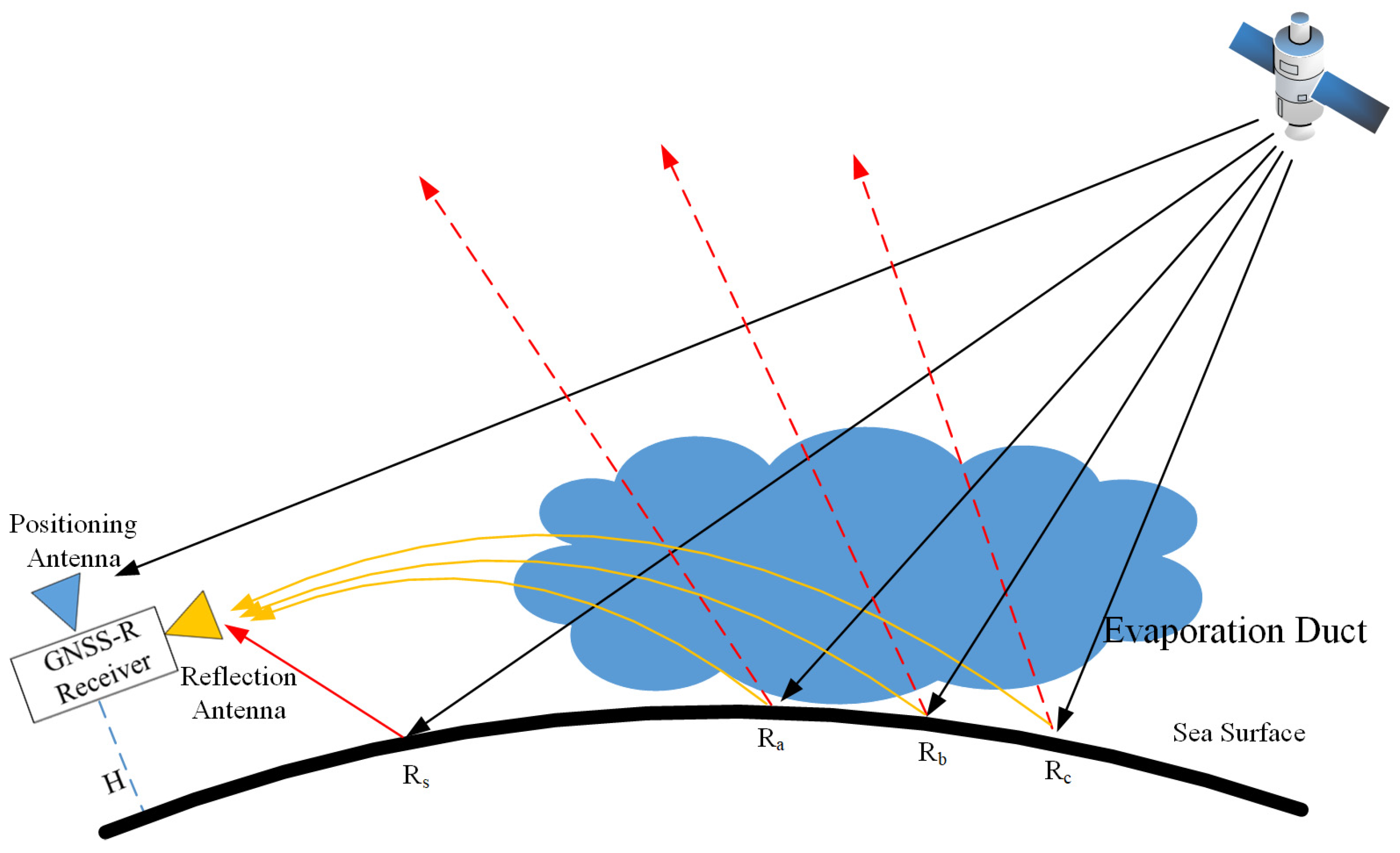
Figure 1 provides an illustration of the effect of an evaporation duct on GNSS-R observations. When GNSS signals are reflected by the sea surface, a portion of the signals undergo specular reflection, which can be modeled using optical principles, while the remaining signals are scattered randomly. Under normal atmospheric conditions over the sea, with a reflection antenna positioned on a coastal station or ship, only the reflected signal around the specular point (denoted as $R_s$) can be received. However, in the presence of an evaporation duct, additional reflected signals from the sea surface (denoted as $R_a$, $R_b$, and $R_c$), which would otherwise be unreachable under normal atmospheric conditions, can be received due to the refractive effect of the evaporation duct.

Based on the specified evaporation duct parameters, the atmospheric refractive index for each layer is computed by utilizing a spherical layered model. The receiver’s location is designated as the signal transmission source, from which light is emitted at various angles. The trajectory of each emitted light ray is simulated using a ray-tracing algorithm. 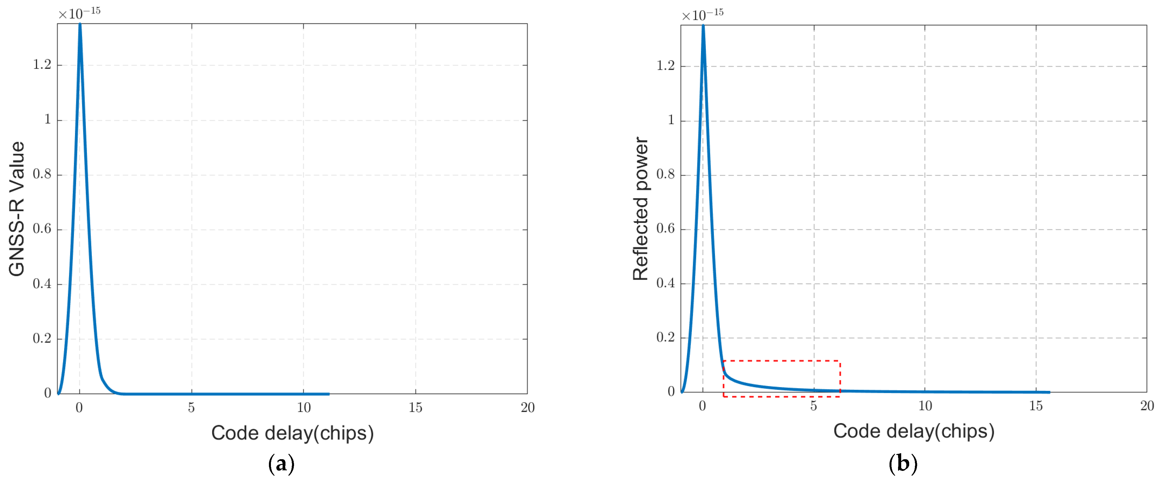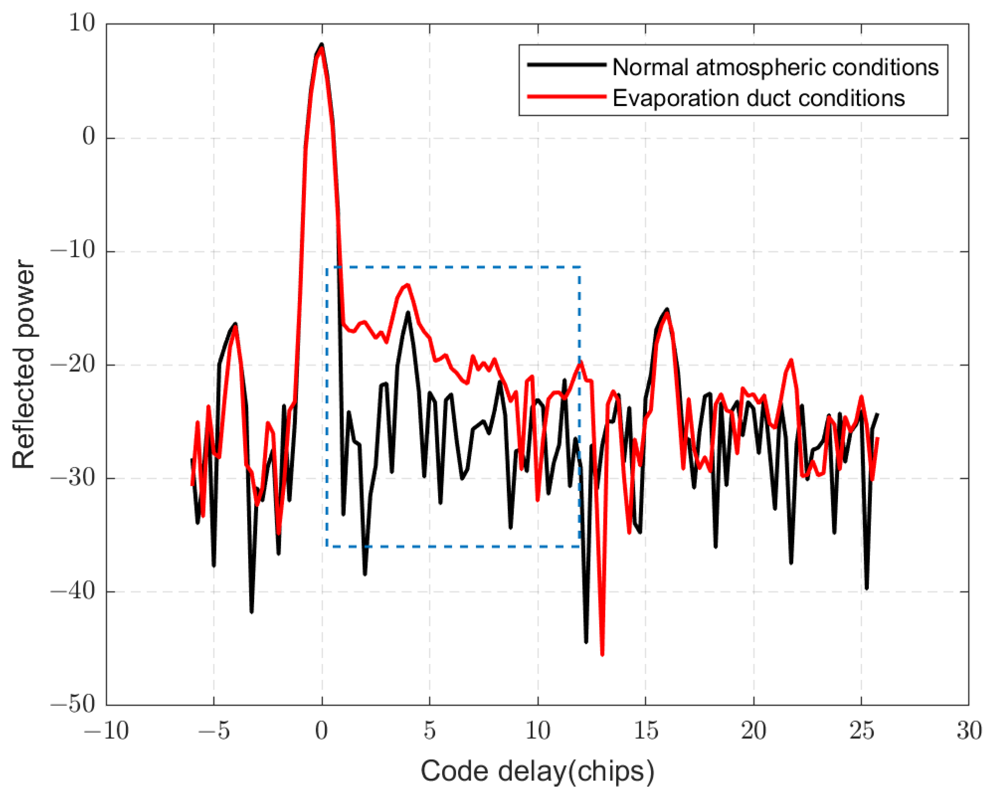When a specific light ray becomes tangent to the Earth’s surface, the point of tangency is identified as the maximum code delay [30]. Then, the reflection waveforms under normal atmospheric conditions and in the presence of an evaporation duct can be simulated using Formula (2), as shown in Figure 2. Although the sea-surface conditions and evaporation duct parameters were simplified, the simulation results can still provide a theoretical framework. As demonstrated in Figure 2, the evaporation duct causes reflection signals from $R_a$, $R_b$, and $R_c$ to produce a distinct rising zone marked by a red rectangle in the DM.

It is worth noting that the theoretical simulation in Figure 2 did not consider autocorrelation effects. Although the attenuation of the GNSS-R signals within an evaporation duct is lower than that in the normal atmosphere, only a portion of the scattered signal can be received due to the incidence angle. This results in the GNSS-R signal power outside the specular point being significantly weaker than that in the specular point itself. One of the most important challenges is that of detecting these weaker GNSS-R signals.

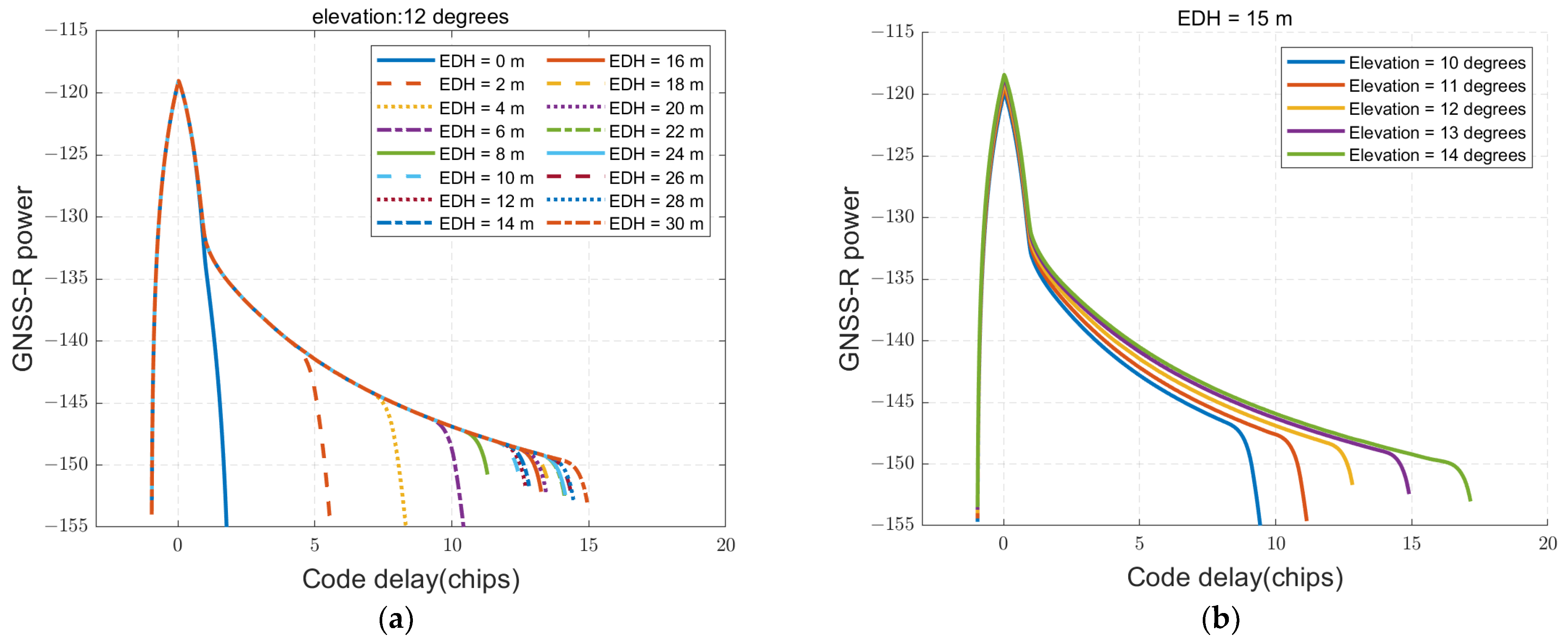
Through simulation studies, it was found that the range of the rising zone was closely related to the evaporation duct parameters, particularly the evaporation duct height and the elevation angle of the satellite corresponding to the received signal. As shown in Figure 3, the range of the rising zone increases monotonically with both the evaporation duct height and the satellite elevation angle. The relationship between the code delay and evaporation duct height is nonlinear. As the evaporation duct height increases, the change in the code delay becomes less pronounced, leading to varying detection accuracies across different heights. Consequently, an optimal elevation observation range exists for engineering applications. The simulation results indicate that higher evaporation duct heights enable the reception of reflected signals over a broader range. However, as the reflection point moves farther from the receiver, the signal power diminishes due to increased propagation distance and greater power loss. When the evaporation duct height is particularly low, the code delay range of the received reflected signal is smaller, making it more discernible in the waveform. However, this smaller range is more susceptible to interference from other multipath signals. Conversely, if a multipath signal with a large code delay is consistently received, it is likely attributable to the evaporation duct. However, when the evaporation duct height exceeds a certain threshold, the reflection waveform changes become less distinct, making retrieval challenging. Therefore, until significant advancements are made in theory or engineering technology, there will remain a more suitable range for evaporation duct retrieval. If the range of the reflected signals can be accurately detected in the presence of an evaporation duct, the evaporation duct height can be inverted, as the elevation of the satellite can be precisely determined by the receiver. The functional relationship can be expressed as follows:

$$h_{ED}=f\left({\tau }_e,\theta \right)$$

(4)

where $h_{ED}$ is the evaporation duct height (unit: m), ${\tau }_e$ is the maximum code delay (unit: L1C/A code chip), and $\theta$ is the elevation angle of the GNSS.

2.3. Semi-Physical Simulation

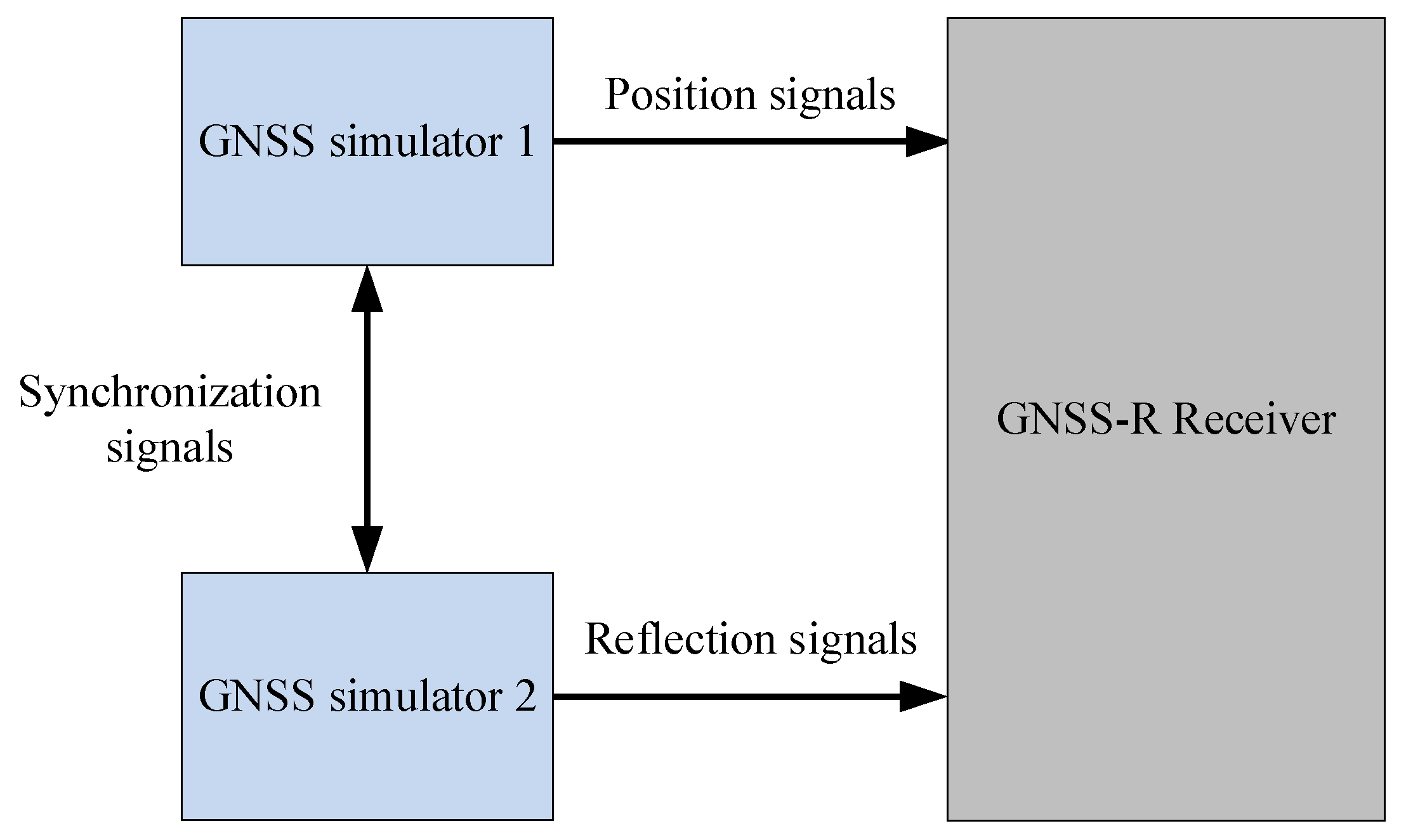
A GNSS simulator is a valuable tool for GNSS receiver development, as it can generate actual GNSS signals based on user-defined configurations. As illustrated in Figure 4, at least two simulators are required for GNSS-R simulations: one to simulate the direct signal and the other to simulate the reflected signal. The reflected signal can be modeled as a combination of multiple multipath signals with varying delays [26]. The connection between the simulators and the GNSS-R receiver is carefully configured to replicate real-world signal propagation conditions.

The semi-physical simulation builds upon the theoretical simulation. Initially, the maximum code delay is simulated theoretically under specified evaporation duct parameters. Subsequently, all reflected signals, ranging from the specular point to the maximum code delay, are discretized and simulated. For instance, discrete multipath signals are generated at equal intervals. Finally, the simulation interval is determined based on the number of multipath signals that the simulator can effectively replicate.

The GSS9000 is a multifunctional GNSS simulator capable of generating up to 16 channels of multipath signals. In our semi-physical simulation, the reflected GNSS signal is approximated using multipath signals with equal intervals of code delay. In particular, 16 multipath signals are simulated by the GSS9000 under both normal atmospheric conditions and evaporation duct scenarios, with GPS L1C/A signals being the primary focus. The resulting DMs received by the GNSS-R receiver are as follows.

As Figure 5 shows, under normal atmospheric conditions, the DM data exhibit a main peak at the specular point, accompanied by minor autocorrelation peaks. In the presence of multipath signals, the DM of GPS displays an increase in signal power following the main peak. The semi-physical simulation results align closely with those of the theoretical simulation presented in Figure 2. However, reflected signals outside the specular point are relatively weak, with the signal power being comparable to or even lower than that of the autocorrelation peaks. Additionally, GNSS reflection signals in non-specular regions interact with the autocorrelation peaks, leading to an increase in the amplitude of trailing autocorrelation peaks. It should be noted that autocorrelation affects DMs, so it is necessary to eliminate autocorrelation interference during data processing.

3. Experimental Design and Data Processing

3.1. Experimental Instruments

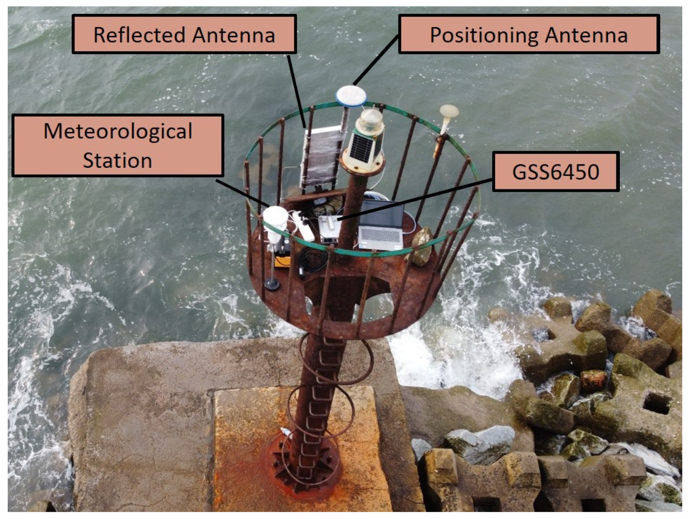
From the results described in Section 2, it can be seen that it is possible to detect evaporation ducts using GNSS-R observations. To investigate the feasibility of this method, an experiment was conducted at a dock in Qinhuangdao, Hebei Province, China. An observation platform approximately 6 m above sea level was selected for the experiment. As shown in Figure 6, a Right-Hand Circularly Polarized (RHCP) antenna (National Space Science Center, Chinese Academy of Sciences (NSSC/CAS), Beijing, China) was installed to capture direct GNSS signals (referred to as position signals), while a Left-Hand Circularly Polarized (LHCP) antenna (NSSC/CAS, Beijing, China) was positioned parallel to the sea surface to collect scattered GNSS signals (referred to as reflection signals). It is well known that reflection signals are generally weaker than direct signals, and signals reflected from non-specular points are even weaker due to increased transmission losses over longer distances. Therefore, antenna gain played a critical role in determining the quality of the experimental results. The LHCP antenna used in this experiment was a high-gain antenna, providing over 10 dB of gain within a horizontal range of ±20 degrees. The GNSS receiver used in the experiment was a commercial software receiver, the GSS6450 (Spirent Communications plc, Paignton, the United Kingdom), capable of simultaneously recording both position and reflection signals. The receiver was configured with a sampling bit width of 8 bits and a bandwidth of 30 MHz.

The positioning antenna captured data stored in the 6450 positioning channel, while the reflecting antenna captured data stored in the 6450 reflecting channel. After completing the outdoor experiment, the data recorded by GSS6450 were utilized as the signal source. This process introduced some losses during sampling and output. These data were then processed by a hardware receiver developed by the NSSC/CAS. This receiver was capable of simultaneously processing reflection signals from BDS B1C, GPS L1C/A, and GALILEO E1. It operated with a code resolution of 1/4 chip and a delay range of [−6, 26] chips. The receiver processed the positioning signal to determine the position, calculated the elevation of the GPS satellite, and predicted the reflecting satellite based on the positioning results. Subsequently, the receiver’s reflection channel computed the code delay and Doppler delay of the specular point. Using these calculations, the receiver correlated the reflected signal to obtain the reflected DM data, which were then further processed.

3.2. Acquisition of Data for Evaporation Duct Comparison

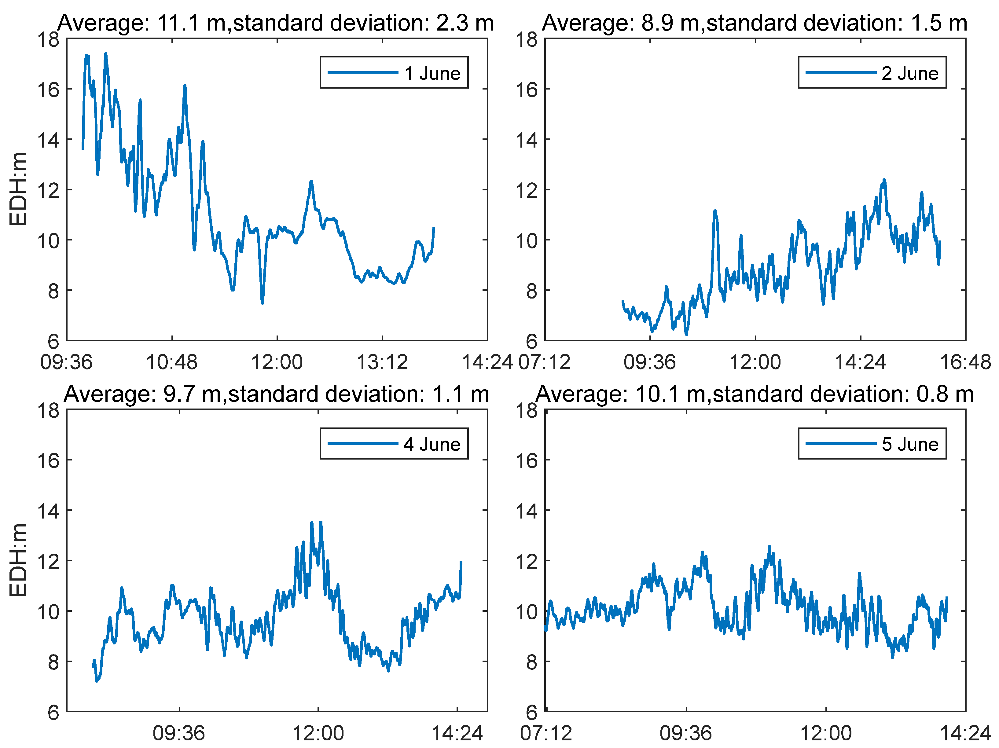
As illustrated in Figure 6, the test platform was equipped with an automatic meteorological station capable of providing atmospheric parameters, including air temperature, humidity, wind speed, and atmospheric pressure, at an update rate of 1 Hz. The actual height of the evaporation duct was estimated using the PJ model, a widely recognized prediction model initially proposed by Jeske in 1973 [31] and later modified by Paulus in 1985 [32]. The PJ model is considered to be one of the most widely used in the world, primarily due to its simplicity and efficiency in calculation. The PJ model operates under the assumption that air parameters are measured at a height of 6 m and that the atmospheric pressure is 1000 hPa. 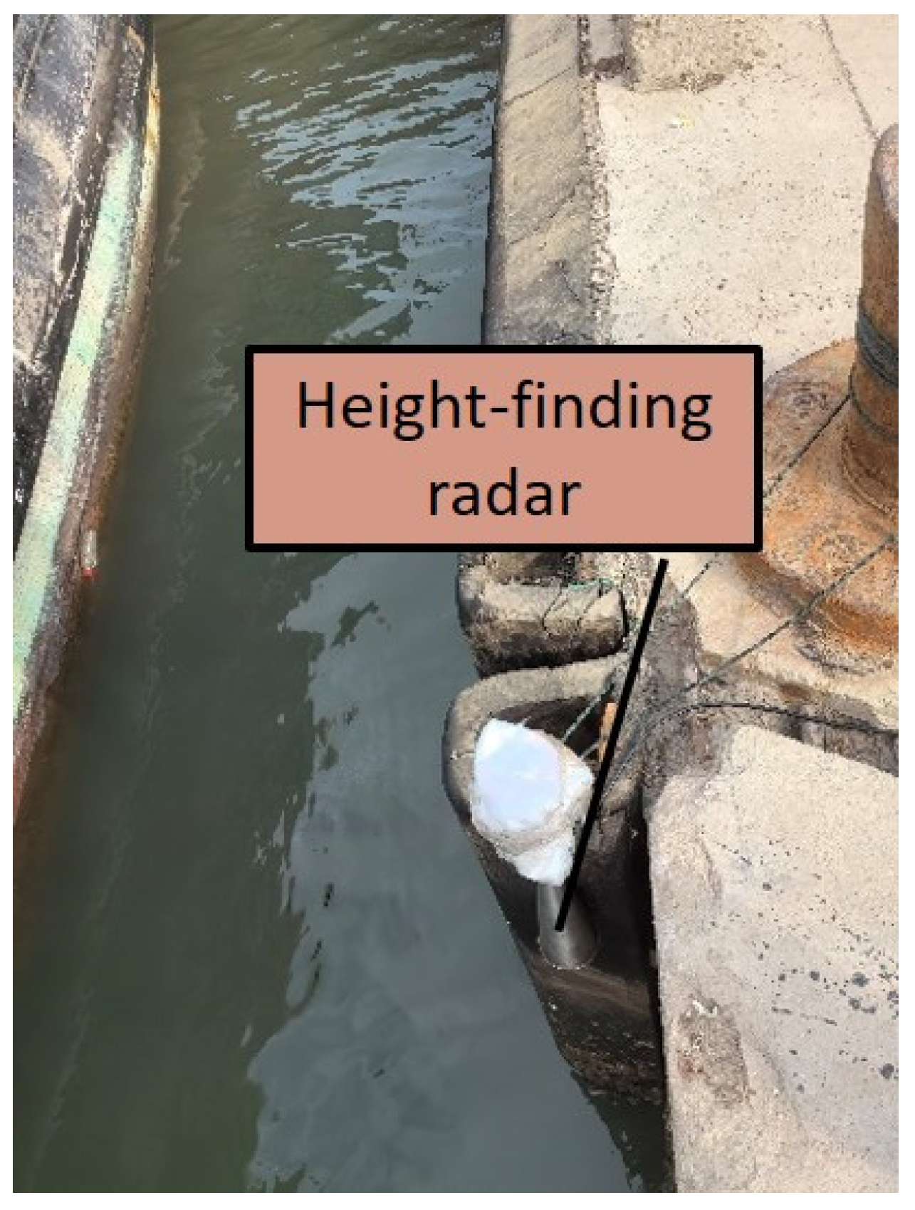The specific calculation steps are provided in Appendix A, while the detailed derivation process can be found in the referenced literature [31,32]. To adapt the model to this experiment, the sea-surface height was incorporated as a parameter. A radar system was installed at the dock to continuously monitor the distance between the sea surface and the platform’s base, as shown in Figure 7.

During the experiment, the distance between the sea surface and the platform base varied from 0.51 m to 1.45 m. The automatic meteorological station was positioned at a height of 4.76 m from the base of the platform. This configuration placed the automatic meteorological station at an approximate altitude of 6 m above the sea surface, thereby rendering the PJ model applicable within the experimental framework. However, it should be noted that the PJ model requires sea-surface temperature (SST) as an input parameter, in addition to air parameters. For this experiment, SST data from ERA5 of the European Center for Medium-Range Weather Forecasts (ECMWF) were utilized, despite the acknowledgment that employing SST from ECMWF may lead to an underestimation of the EDH [33]. Nevertheless, utilizing SST from ECMWF remains a valuable approach for EDH estimation.

3.3. Incoherent Integration

In order to estimate GNSS scintillation and improve the signal-to-noise ratio (SNR), incoherent integration is a necessary step in processing DM data, in addition to coherent integration. In a typical GNSS-R receiver, the incoherent integration time is typically 1 s. However, considering the weak GNSS-R signals outside of the specular point, a longer incoherent integration time may be more effective.

A GNSS signal can be described as follows:

$$s\left(t\right)=Ap\left(t\right)\sin \left(2\pi ft\right)$$

(5)

where $A$ is the amplitude of the GNSS signal, $p$ is the power of the signal, and $f$ and $t$ are the frequency and time of the signal, respectively.

Thus, all scattered signals contribute to the final received signals. In other words, each signal acts as a multipath signal for the selected signal, and the final signal can be described as follows [34]:

$$s_{all}\left(t\right)=Ap\left(t\right)\sin \left(2\pi ft\right)+{\displaystyle \sum _{i=2}^L\left({\alpha }_{i}Ap\left(t-{\tau }_i\right)\sin \left(2\pi ft+{\varphi }_i\right)\right)}+\epsilon$$

(6)

where $\alpha$ is the attenuation coefficient of multipath signal, $i$ is the multipath number, $\tau$ is the delay of the multipath to the selected signal, $\varphi$ is the phase change in the multipath to the selected signal, and $\epsilon$ is the total noise.

In $N$ incoherent integrations, Equation (6) is rewritten as follows:

$${\displaystyle \sum _{j=1}^N{s}_{all}\left(t\right)}={\displaystyle \sum _{j=1}^{N}Ap\left(t\right)\sin \left(2\pi ft\right)}+{\displaystyle \sum _{j=1}^N{\displaystyle \sum _{i=2}^L\left({\alpha }_{i}Ap\left(t-{\tau }_i\right)\sin \left(2\pi ft+{\varphi }_i\right)\right)}}+\epsilon$$

(7)

All of the scattered signals contribute to the final signal in this way. Incoherent integration reduces the influence of noise.

For most GNSS-R receivers, the coherent time is generally less than 20 ms due to the length of the navigation message. In this study, we use a 10 ms coherent time to increase the reflected signal power. The total gain of a receiver $G_{all}$ can be described as follows:

$$G_{all}=G_{coh}+G_{ncoh}$$

(8)

where $G_{coh}$ is the gain of coherent integration, and $G_{ncoh}$ is the gain of incoherent integration.

The power of the reflected signal is typically weaker than that of the direct signal due to energy loss during sea-surface reflection and the longer propagation distance, which further attenuates the signal. The power gain achieved through coherent integration can be expressed as follows:

$$G_{coh}=10\lg \left(B_{pd}{T}_{coh}\right)$$

(9)

where $B_{pd}$ is the noise bandwidth, and $T_{coh}$ is the coherent time. If $B_{pd}$ and $T_{coh}$ are 2 MHz and 10 ms, respectively, then $G_{coh}$ is about 43 dB.

Incoherent integration can enhance signal power without significantly increasing the computational complexity, but incoherent integration can introduce square loss $G_{nc}$. The considered square loss can be written as follows:

$$G_{nc}=10\lg N_{nc}-L_{sq}$$

(10)

where $N_{nc}$ is the time of incoherent integration, and $L_{sq}$ is the square loss.

To estimate the best time for incoherent integration, the reflected signal power must be accurately estimated. However, this is almost impossible, as the sea surface and the evaporation duct conditions are unknown. If a higher SNR is expected, more incoherent time is required.

3.4. Autocorrelation Elimination

In an evaporation duct environment, scattered signals from non-specular points can be received by a GNSS-R receiver, but their power is attenuated due to the limited field of view of the antenna and the increased propagation distance. As is well known, GNSS signal strength is lower than noise, thus requiring correlation techniques for detection. Similarly, GNSS-R signals are generally weaker than direct GNSS signals. While the evaporation duct environment enhances the reception of GNSS-R signals, their strength remains close to the autocorrelation noise level. In other words, autocorrelation is a major obstacle to the detection of evaporation ducts using GNSS-R.

Although there is a proportional relationship between main peaks and autocorrelation peaks, this method can partially remove autocorrelation interference [35]. Fortunately, the position of the autocorrelation peak is fixed, and it can be used to eliminate autocorrelation interference.

4. Results

4.1. PJ Model

In a four-day experiment performed on 1, 2, 4, and 5 June 2024, the air temperature, relative humidity, and wind speed were collected at a meteorological station. Based on the location of the experimental site, the sea-surface temperature data from ERA5 were selected using the nearest-neighbor method, and the EDH was subsequently calculated using the PJ model. The EDH results obtained during the experiment are shown in Figure 8. Based on the evaporation ducts derived from meteorological data, evaporation ducts existed in the four-day experiment with average heights of 11.1 m, 8.9 m, 9.7 m, and 10.1 m, respectively. The standard deviation of the EDH reflects the stability of the evaporation duct, indicating the most stable conditions on 5 June and the most significant variations on 1 June. In this study, it was assumed that the evaporation ducts were consistent in the horizontal direction, so the EDH calculated with the PJ model could describe the parameters on the sea surface.

4.2. DM Data of Evaporation Ducts

In the four-day experiment, four sets of raw data were recorded by the GSS6450 receiver. According to the simulation results in Section 2.2, the reflected signal transmitted in the evaporation duct has a power reduction of more than 30 dB compared with the signals reflected from the specular point. Consequently, several methods must be considered to obtain a complete reflection waveform. As discussed in Section 3.3, coherent and incoherent integration is a critical method for enhancing signal gain. In addition, the antenna plays a significant role in the signal processing. In the experiment, the reflected antenna had a maximum gain of more than 10 dB, with the azimuth corresponding to this maximum gain at 135 degrees (except on 1 June, when the azimuth for the maximum gain was 115 degrees).

In this study, a coherent integration time of 10 ms and an incoherent accumulation of 10,000 iterations were employed, corresponding to data processing intervals of 100 s. Following incoherent accumulation, the data for each 100 s interval were transformed using Equation (11) to enhance visualization. The results of continuous observations over 800 s on 1, 2, 4, and 5 June are presented in Figure 9, Figure 10, Figure 11 and Figure 12, respectively. For the reflection waveform, a trend term was fitted for the data with a code delay greater than 1.5, represented by a red dotted line.

$$P_r=10{\log }_{10}\left({\displaystyle \frac{V_m-{\overline{V}}_n}{{\overline{V}}_n}}\right)$$

(11)

where $V_m$ is the measurement of DMs, and ${\overline{V}}_n$ is the mean value of the noise floor.

As shown in Figure 9, Figure 10, Figure 11 and Figure 12, an autocorrelation elimination algorithm was applied to mitigate the influence of autocorrelation. As illustrated in

Table 1. Average EDH for selected times during the experiment.

SOW of 1 June	Average EDH:m	SOW of 2 June	Average EDH:m	SOW of 4 June	Average EDH:m	SOW of 5 June	Average EDH:m
[533,746 to 533,845]	10.2	[13,885 to 13,984]	8.1	[185,480 to 185,579]	10.7	[271,780 to 271,879]	10.8
[533,846 to 533,945]	10.2	[13,985 to 14,084]	8.1	[185,580 to 185,679]	10.7	[271,880 to 271,979]	10.7
[533,946 to 534,045]	10.2	[14,085 to 14,184]	8.1	[185,680 to 185,779]	10.7	[271,980 to 272,079]	10.7
[534,046 to 534,145]	10.2	[14,185 to 14,284]	8.1	[185,780 to 185,879]	10.7	[272,080 to 272,179]	10.7
[534,146 to 534,245]	10.2	[14,285 to 14,384]	8.1	[185,880 to 185,979]	10.7	[272,180 to 272,279]	10.7
[534,246 to 534,345]	10.2	[14,385 to 14,484]	8.1	[185,980 to 186,079]	10.7	[272,280 to 272,379]	10.6
[534,346 to 534,445]	10.2	[14,485 to 14,584]	8.1	[186,080 to 186,179]	10.7	[272,380 to 272,479]	10.6
[534,446 to 534,545]	10.2	[14,585 to 14,684]	8.1	[186,180 to 186,279]	10.7	[272,480 to 272,579]	10.6

, the average EDH in Figure 9, Figure 10, Figure 11 and Figure 12 is about 10.2~10.8 m, except for that on 2 June, which is about 8.1 m. The experimental results show a significant rise in the reflected waveform on 1 June, 2 June, and 5 June. However, there is no significant rise on 4 June, except for the second of the week (SOW) [185,480 to 185,579] of the GPS time. This anomaly may be attributed to signal interference or an uneven distribution of the evaporation duct on 4 June, resulting in the attenuation of the GNSS signal when passing through the evaporation duct area. As previously analyzed, the reflected signal power in the duct area is very low, making it susceptible to noise and difficult to capture. Further experiments and related research are required to explore this phenomenon in greater detail.

Although a continuously rising DM was observed on 1 June and 2 June, the amplitude of the rising zone was smaller than that on 5 June, particularly at the edges, where the signal was significantly affected by noise. The reason may be that the EDH calculated with the PJ model may have been inaccurate, or the actual evaporation duct height and its horizontal distribution were uneven. In addition, the hardware configuration of the GSS6450 differed across the experimental days. On 1 June and 2 June, radio frequency (RF) port 2 was connected to the positioning antenna with an external feed, while RF port 1 was connected to the reflection antenna through a filter. On 4 June and 5 June, RF port 2 was employed for reflection signal acquisition with a gain of 27 dB. On 4 June, RF port 1 was connected to the positioning antenna with an external feed, while RF port 1 directly fed the positioning antenna on 5 June. These variations in hardware connections may have contributed to inconsistent signal quality, particularly the lack of a significant rise on 4 June. Furthermore, as indicated by the standard deviation of the evaporation duct height derived from the meteorological parameters (shown in Figure 8), the evaporation duct on 5 June was the most stable. This stability likely minimized the impact of environmental fluctuations on the reflected signal during incoherent accumulation, potentially explaining why the most pronounced data rise was observed on 5 June.

4.3. Retrieval Attempt from DM Data

The simulation results indicate that the presence of evaporation ducts leads to a distinct edge in the DM. In order to invert the EDH from the DM, a simulation was performed to calculate the ideal EDH value. Then, based on the simulation results, a fitting relationship can be established for Formula (4) as follows:

$$\left\{\begin{array}{l}{h}_{ED}=6.699\times {10}^{-15}\times \exp (0.216\times R_s)+0.4156\times \exp (0.02371\times R_s)\hfill \\ R_s=p_2\left(\theta \right)\times {\tau }_e^2+p_1\left(\theta \right)\times {\tau }_e+p_0\left(\theta \right)\hfill \\ p_2=-7388.884\times {\theta }^{-4.482}+0.002405\hfill \\ p_1=1659.928\times {\theta }^{-1.94}-0.1325\hfill \\ p_0=14.435\times {\theta }^{-1.686}+0.001322\hfill \end{array}\right.$$

(12)

where $R_s$ is the effective scattering radius (unit:km).

Since the uplift of the waveform on 5 June is obvious, we selected one of the data in Figure 13 to discuss the feasibility of inversion. Although this inversion is not accurate, it can still provide some reference for future research.

According to Formula (12), the retrieval requires the elevation information of GNSS and the maximum code delay of the uplift area in the reflected waveform. The DM for 5 June, which was processed to eliminate autocorrelation, is selected as an example in Figure 13. When the receiver processes the positioning signal, accurate elevation information can be obtained from the ephemeris file. The primary challenge lies in the effective identification of the maximum code delay. Due to the power of the reflected signal uplift region induced by the evaporation duct—which is even lower than the autocorrelation power—the boundary between the maximum code delay and the noise floor becomes difficult to distinguish. The data before the specular point can be regarded as noise, thus providing a reference for the noise level for edge detection. Then, the code delay can be obtained from the actual DM. The edge of the signal in Figure 13 is difficult to estimate, so a possible boundary is selected as an example, which is approximately 12.25 chips. However, we cannot obtain an accurate edge of the DM rise zone in Figure 13 because the signal at the edge is very weak and close to the noise. The total gain in our experiment is limited by the coherent integration, incoherent integration, and antenna, which cannot provide sufficient gain to make the signal much greater than the noise. In the example given in Figure 13, the elevation of GPS PRN9 is from 13.18 degrees to 13.71 degrees; only the signal of the maximum elevation angle results in the farthest signal boundary, and this also makes the edge much closer to the noise. Then, according to the inversion fitting formula in (12), the EDH retrieval value according to GNSS-R is 6.6 m. The average height of the evaporation duct calculated using the meteorological parameters in the corresponding time period is 10.6 m. Therefore, the retrieval error is 4 m for this case.

The possible error sources in the above retrieval are as follows. (1) Signal-noise ratio limitations: Due to factors such as antenna gain and environmental interference, the useful signal may be lower than the noise floor in the DM received by the receiver. As a result, the identified maximum code delay will not be the true signal boundary, and this will lead to inaccurate retrieval results. (2) Theoretical model: There are some errors between the theoretical simulation model and the actual situation. The theoretical simulation only considers some main parameters while neglecting the influence of additional factors such as evaporation duct strength and wind speed, thus introducing inversion fitting errors. (3) PJ model error: The PJ model based on meteorological parameters for predicting the EDH has some errors between the predicted EDH and the actual EDH. (4) Horizontal distribution of evaporation ducts: An actual evaporation duct may have a non-uniform horizontal distribution, which is not accounted for in the theoretical simulations or the measured meteorological reference data used in this study. This oversight may introduce additional errors. (5) Code delay resolution: During the processing of DMs, the code delay resolution is 1/4 of a chip. This resolution constraint may also contribute to errors in the retrieval results.

Although accurate retrieval results could not be obtained in this experiment due to limitations such as antenna gain, this attempt still represents a possible retrieval method.

5. Discussion

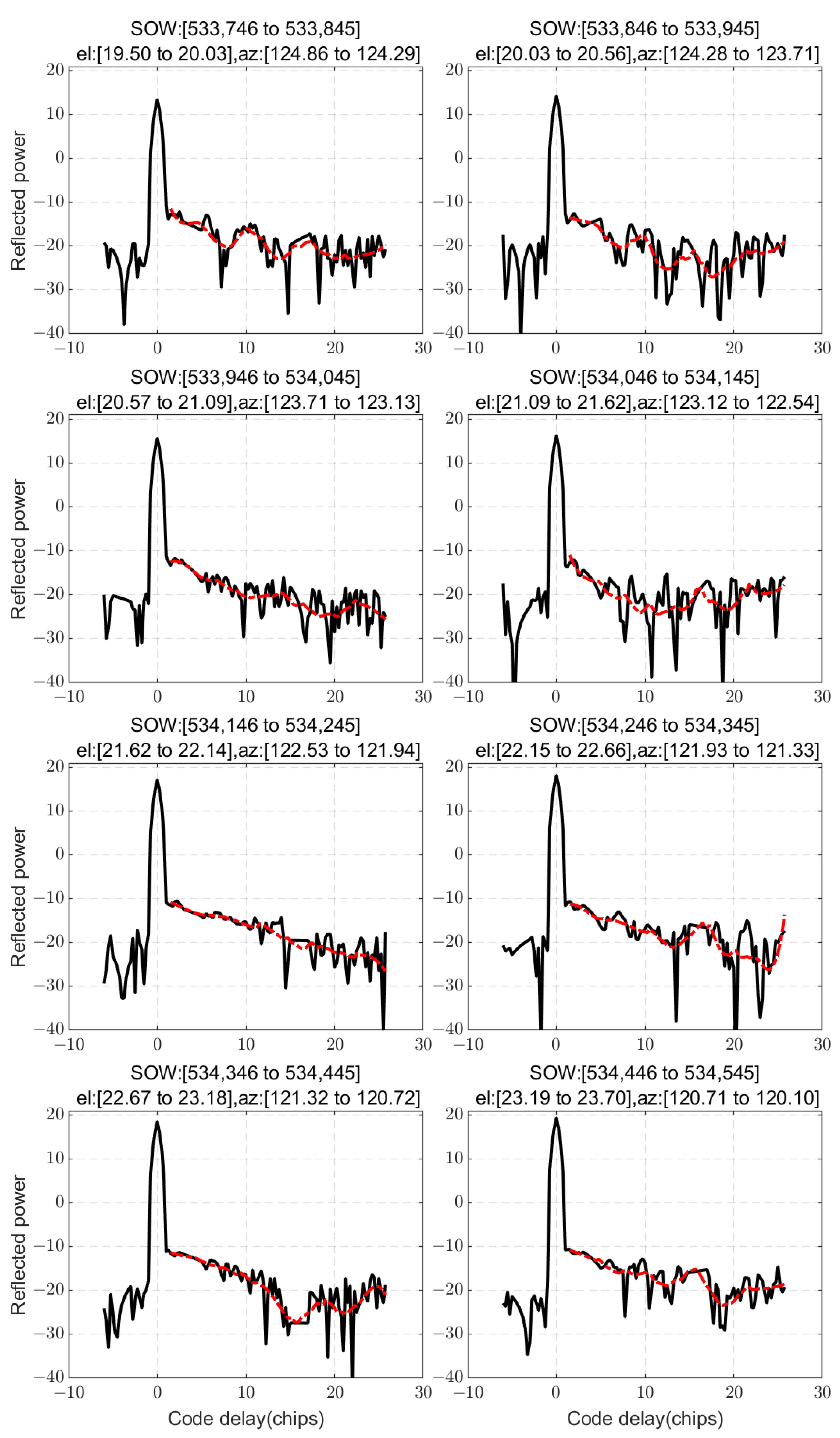
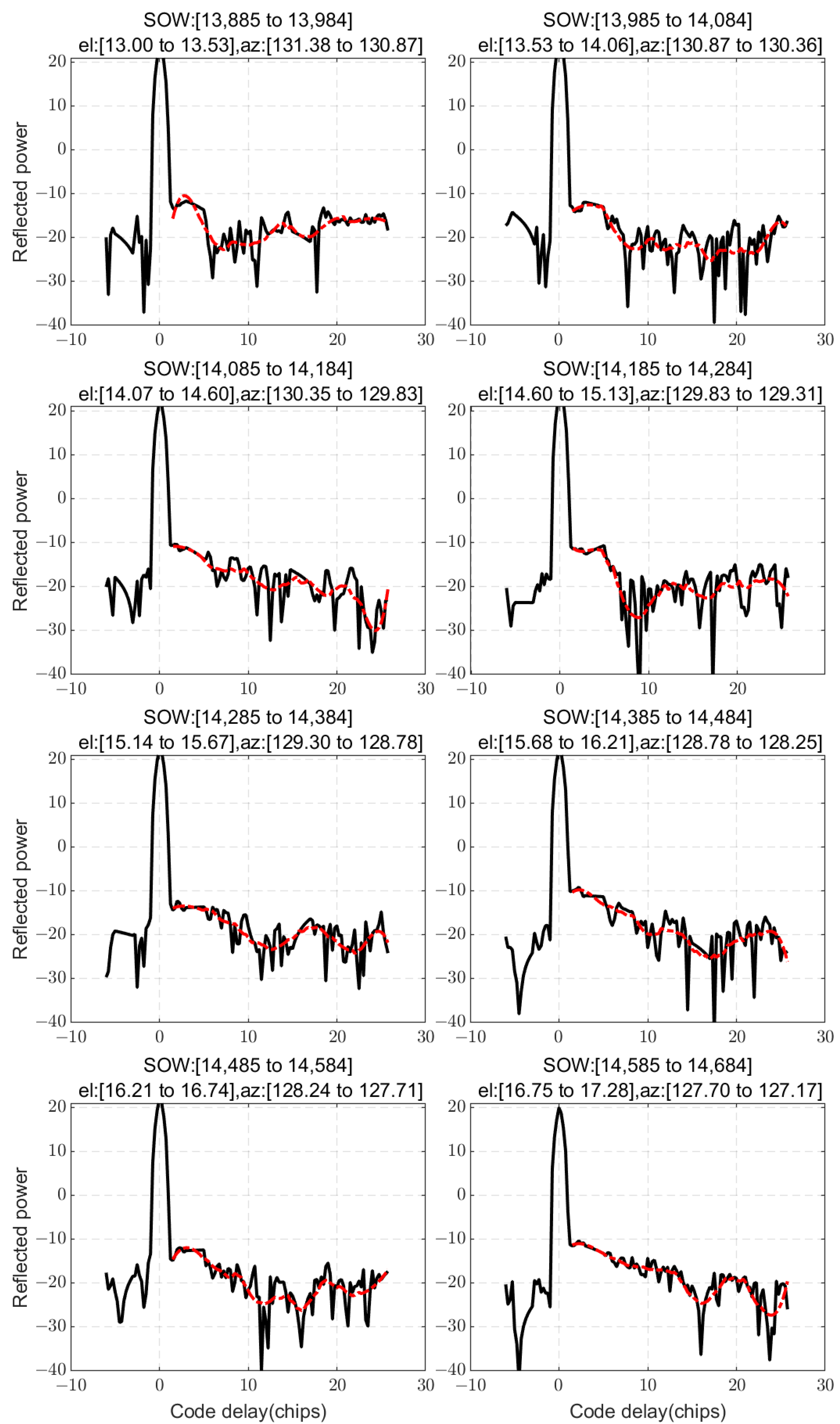
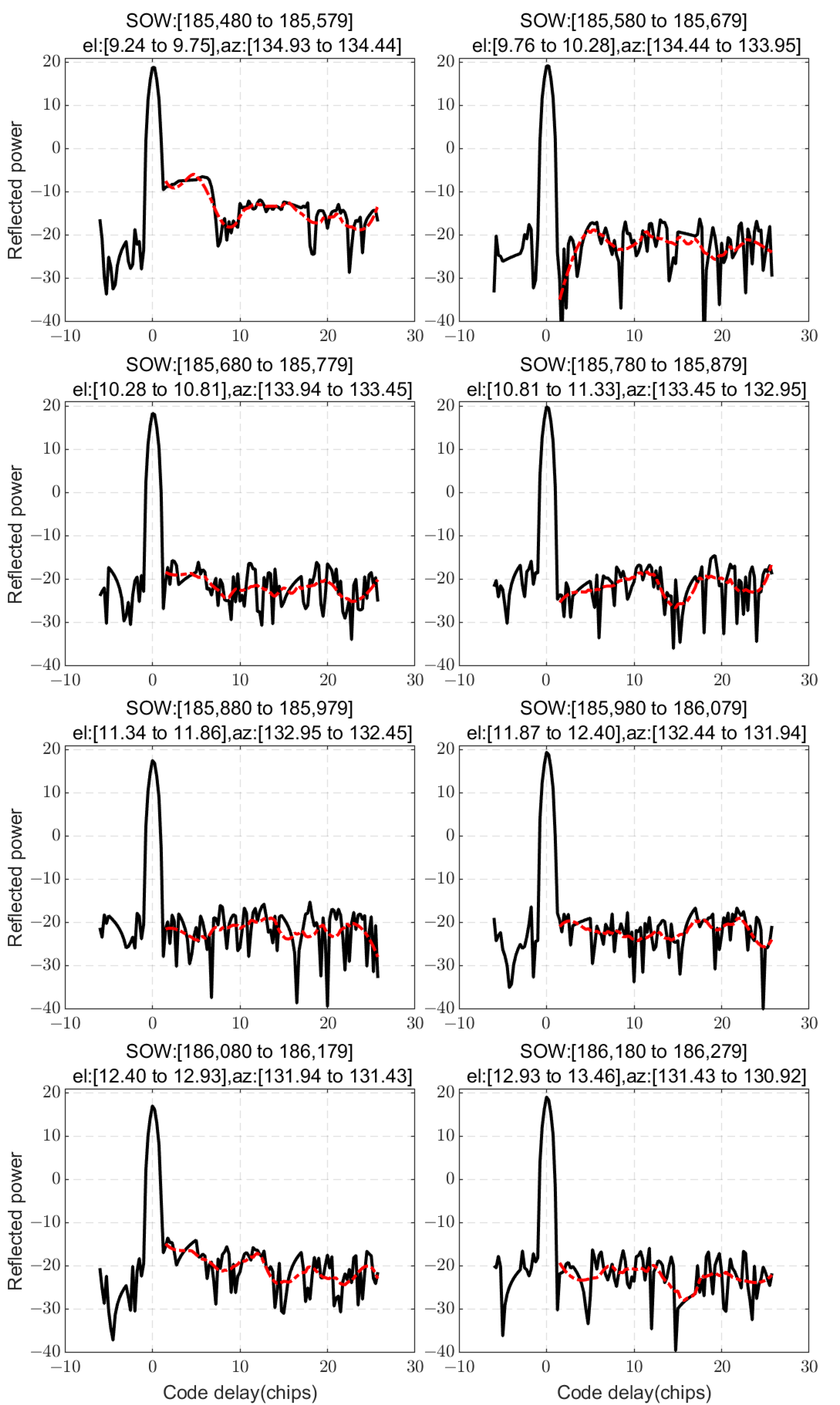
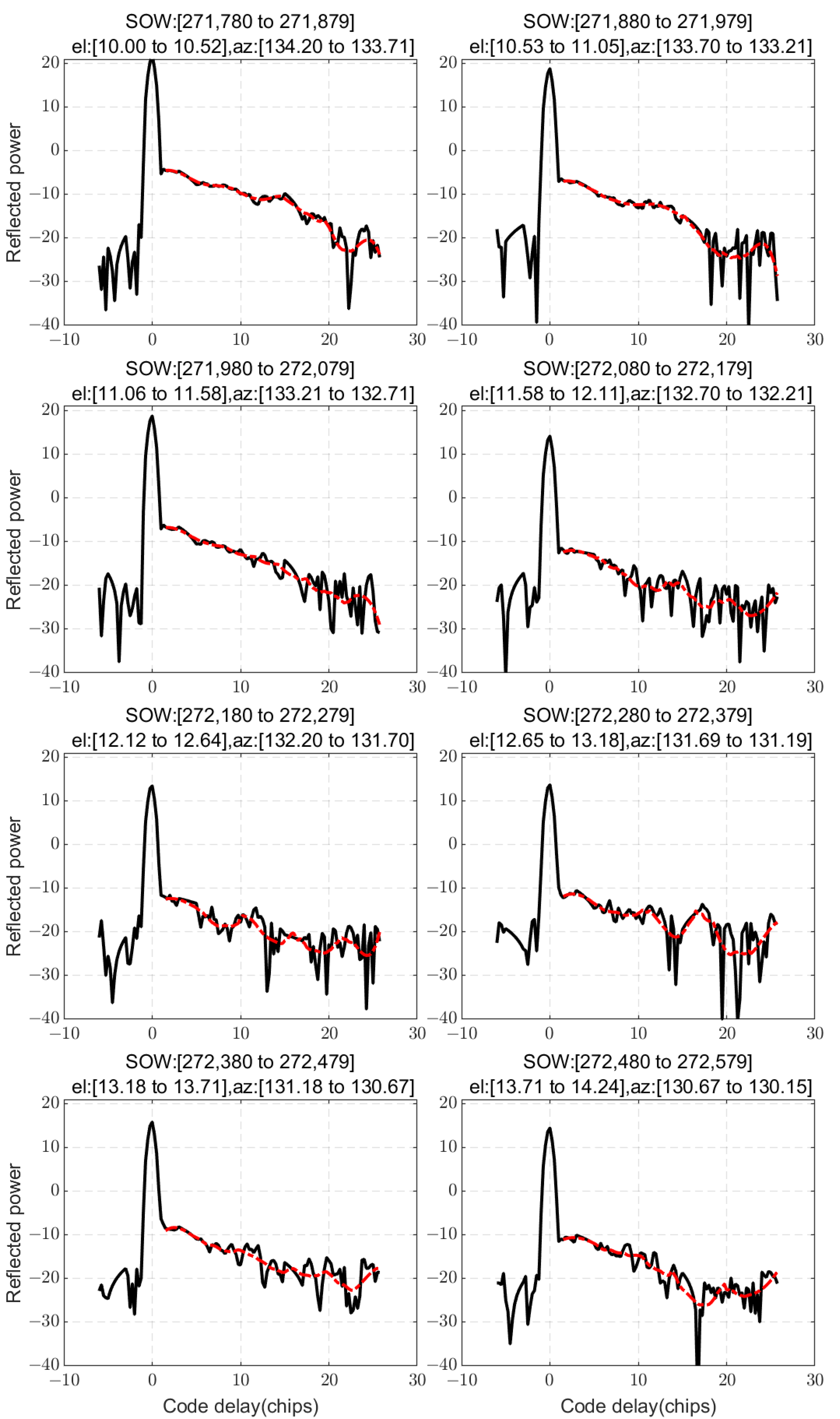
An evaporation duct causes the atmospheric refractive index to exceed the curvature of the Earth, thereby altering the propagation trajectory of electromagnetic waves. Consequently, when a reflected GNSS signal passes through an evaporation duct region, the propagation path of the reflected GNSS signal will be changed, enabling signals that are beyond the line-of-sight transmission range in a standard atmospheric environment to reach the reflecting antenna and be received by the GNSS-R receiver. This phenomenon is evident in GNSS-R DMs, where the presence of an evaporation duct induces a noticeable rise in DMs. Therefore, GNSS-R has potential for the retrieval of evaporation ducts, and this study mainly demonstrates this possibility.

In this study, through a theoretical simulation, semi-physical simulation, and experiment, a rise in DMs in the presence of evaporation ducts is demonstrated. The theoretical simulation results demonstrate a monotonic relationship between the EDH and the maximum code delay in the rising region of the reflection waveform. This relationship enables the retrieval of GNSS-R DMs by leveraging this correspondence along with other relevant parameters. The semi-physical simulation results demonstrate that the autocorrelation peak position aligns with theoretical calculations, confirming the reliability of this approach. Compared to purely theoretical simulations, semi-physical simulations can more accurately replicate complex real-world factors such as random noise, thereby generating signals that better approximate actual environmental conditions. Furthermore, the experimental results, supported by the PJ model, demonstrated that the reflected DMs rose in non-specular points when there was an evaporation duct. The reflected DM waveform exhibited multiple instances of rising, providing empirical evidence of a direct correlation between the evaporation duct phenomenon and the observed rise in reflection waveforms.

It is very important and necessary to use GNSS-R signals for inversion. However, due to the limited antenna gain employed in the experiment, only one theoretically feasible retrieval method can be proposed at this stage. The preliminary retrieval of EDH was achieved using DMs from GPS PRN9 in an experimental dataset under the assumption that all signals can be received and detected. Nevertheless, accurate retrieval necessitates additional data and a more comprehensive theoretical model. When all reflected waveforms can be reliably detected above the noise floor, this method may be a considerable potential method.

It should be noted that the simulation model of the reflection signal used in evaporation ducts only considers the evaporation duct height. The strength of the evaporation duct and its complex structure must also be investigated in the future to obtain more accurate retrieval results.

In this work, the signal was recorded in a data recording instrument and subsequently reprocessed by a hardware receiver, resulting in a power loss in the GPS L1C/A signal power in both the direct and reflected paths. Although this power loss can be disregarded for positioning purposes, it represents a significant source of interference for the reflection signal, as the power of the reflection signal propagating through the evaporation duct is weak and within a similar range of autocorrelation. Subsequently, by optimizing the algorithm and improving the hardware receiver, DMs can be collected directly.

The reference evaporation duct data derived from the PJ model were influenced by several factors, such as the accuracy of the meteorological data. We tested the air parameters on a platform on the coast, which could be different from real evaporation duct conditions over the sea surface, and a more precise reference is required in future work.

References

1. Huang, L.F.; Liu, C.G.; Wang, H.G.; Zhu, Q.L.; Zhang, L.J.; Han, J.; Zhang, Y.S.; Wang, Q.N. Experimental Analysis of Atmospheric Ducts and Navigation Radar Over-the-Horizon Detection. Remote Sens. 2022, 14, 17. [Google Scholar] [CrossRef]
2. Shi, Y.; Wang, S.W.; Yang, F.; Yang, K.D. Statistical Analysis of Hybrid Atmospheric Ducts over the Northern South China Sea and Their Influence on Over-the-Horizon Electromagnetic Wave Propagation. J. Mar. Sci. Eng. 2023, 11, 19. [Google Scholar] [CrossRef]
3. Wang, S.W.; Yang, K.D.; Shi, Y.; Yang, F.; Zhang, H. Impact of Evaporation Duct on Electromagnetic Wave Propagation During a Typhoon. J. Ocean Univ. 2022, 21, 1069–1083. [Google Scholar] [CrossRef]
4. Zhang, Q.; Yang, K.D. Study on evaporation duct estimation from point-to-point propagation measurements. IET Sci. Meas. Technol. 2018, 12, 456–460. [Google Scholar] [CrossRef]
5. Yang, C. Estimation of the Atmospheric Duct from Radar Sea Clutter Using Artificial Bee Colony Optimization Algorithm. Prog. Electromagn. Res. 2013, 135, 183–199. [Google Scholar] [CrossRef]
6. Barrios, A. Estimation of surface-based duct parameters from surface clutter using a ray trace approach. Radio Sci. 2004, 39, 1–9. [Google Scholar] [CrossRef]
7. Zhang, J.P.; Wu, Z.S.; Zhang, Y.S.; Wang, B. Evaporation Duct Retrieval Using Changes in Radar Sea Clutter Power versus Receiving Height. Prog. Electromagn. Res. 2012, 126, 555–571. [Google Scholar] [CrossRef]
8. Zhao, X.F.; Huang, S.X. Estimation of Atmospheric Duct Structure Using Radar Sea Clutter. J. Atmos. Sci. 2012, 69, 2808–2818. [Google Scholar] [CrossRef]
9. Zhao, X.F.; Huang, S.X.; Wang, D.X. Using particle filter to track horizontal variations of atmospheric duct structure from radar sea clutter. Atmos. Meas. Tech. 2012, 5, 2859–2866. [Google Scholar] [CrossRef]
10. Zhao, X.F.; Huang, S.X. Atmospheric Duct Estimation Using Radar Sea Clutter Returns by the Adjoint Method with Regularization Technique. J. Atmos. Ocean. Technol. 2014, 31, 1250–1262. [Google Scholar] [CrossRef]
11. Yang, C.; Guo, L.X. Inferring the atmospheric duct from radar sea clutter using the improved artificial bee colony algorithm. Int. J. Microw. Wirel. Technol. 2018, 10, 437–445. [Google Scholar] [CrossRef]
12. Garrison, J.L.; Katzberg, S.J. The Application of Reflected GPS Signals to Ocean Remote Sensing. Remote Sens. Environ. 2000, 73, 175–187. [Google Scholar] [CrossRef]
13. Zavorotny, V.U.; Voronovich, A.G. Scattering of GPS signals from the ocean with wind remote sensing application. IEEE Trans. Geosci. Remote Sens. 2000, 38, 951–964. [Google Scholar] [CrossRef]
14. Rodriguez-Alvarez, N.; Munoz-Martin, J.F.; Morris, M. Latest Advances in the Global Navigation Satellite System—Reflectometry (GNSS-R) Field. Remote Sens. 2023, 15, 2157. [Google Scholar] [CrossRef]
15. Bu, J.; Yu, K.; Zhu, F.; Zuo, X.; Huang, W. Joint Retrieval of Sea Surface Rainfall Intensity, Wind Speed, and Wave Height Based on Spaceborne GNSS-R: A Case Study of the Oceans near China. Remote Sens. 2023, 15, 2757. [Google Scholar] [CrossRef]
16. Sun, Y.; Huang, F.; Xia, J.; Yin, C.; Bai, W.; Du, Q.; Wang, X.; Cai, Y.; Li, W.; Yang, G.; et al. GNOS-II on Fengyun-3 Satellite Series: Exploration of Multi-GNSS Reflection Signals for Operational Applications. Remote Sens. 2023, 15, 5756. [Google Scholar] [CrossRef]
17. Bai, W.; Wang, G.; Huang, F.; Sun, Y.; Du, Q.; Xia, J.; Wang, X.; Meng, X.; Hu, P.; Yin, C.; et al. Review of Assimilating Spaceborne Global Navigation Satellite System Remote Sensing Data for Tropical Cyclone Forecasting. Remote Sens. 2025, 17, 118. [Google Scholar] [CrossRef]
18. Torres, O.; Katzberg, S.J. Analysis of reflected global positioning system (GPS) signals from land for soil moisture determination and topography mapping. In Proceedings of the Earth Observing Systems VII, Seattle, WA, USA, 7–10 July 2002; pp. 9–15. [Google Scholar]
19. Lwin, A.; Yang, D.; Hong, X.; Zhang, B.; Zhang, B.; Sara, C.S. Opportunity for GNSS Reflectometry in Sensing the Regional Climate and Soil Moisture Instabilities in Myanmar. Climate 2021, 9, 175. [Google Scholar] [CrossRef]
20. Yu, K.; Wang, S.; Li, Y.; Chang, X.; Li, J. Snow Depth Estimation with GNSS-R Dual Receiver Observation. Remote Sens. 2019, 11, 2056. [Google Scholar] [CrossRef]
21. Yu, K.; Li, Y.; Jin, T.; Chang, X.; Wang, Q.; Li, J. GNSS-R-Based Snow Water Equivalent Estimation with Empirical Modeling and Enhanced SNR-Based Snow Depth Estimation. Remote Sens. 2020, 12, 3905. [Google Scholar] [CrossRef]
22. Munoz-Martin, J.F.; Perez, A.; Camps, A.; Ribó, S.; Cardellach, E.; Stroeve, J.; Nandan, V.; Itkin, P.; Tonboe, R.; Hendricks, S.; et al. Snow and Ice Thickness Retrievals Using GNSS-R: Preliminary Results of the MOSAiC Experiment. Remote Sens. 2020, 12, 4038. [Google Scholar] [CrossRef]
23. Ma, W.; Huang, L.; Wu, X.; Jin, S.; Bai, W.; Li, X. Evaluation of CYGNSS Observations for Snow Properties, a Case Study in Tibetan Plateau, China. Remote Sens. 2022, 14, 3772. [Google Scholar] [CrossRef]
24. Wang, B.; Wu, Z.S.; Zhao, Z.W.; Wang, H.G. A Passive Technique to Monitor Evaporation Duct Height Using Coastal GNSS-R. IEEE Geosci. Remote Sens. Lett. 2011, 8, 587–591. [Google Scholar] [CrossRef]
25. Zhang, J.; Wu, Z.; Wang, B.; Wang, H.; Zhu, Q. Modeling low elevation GPS signal propagation in maritime atmospheric ducts. J. Atmos. Sol.-Terr. Phys. 2012, 80, 12–20. [Google Scholar] [CrossRef]
26. Li, B.; Zhang, B.; Yu, Y.; Yang, D.; Peng, B.; Qi, Y.; Wu, D. A Random Model and Simulation for Generating GNSS Ocean Reflected Signals. IEEE Geosci. Remote Sens. Lett. 2019, 16, 1036–1040. [Google Scholar] [CrossRef]
27. Liu, X.; Cao, Y.; Wu, Z.; Wang, H. Inversion for Inhomogeneous Surface Duct without a Base Layer Based on Ocean-Scattered Low-Elevation BDS Signals. Remote Sens. 2021, 13, 3914. [Google Scholar] [CrossRef]
28. Liu, L.J.; Xia, J.M.; Bai, W.H.; Sun, Y.Q.; Du, Q.F.; Luo, L.M. Influence of evaporation duct on the effective scattering region of GNSS reflected signals on the sea surface. Chin. J. Geophys. Chin. Ed. 2019, 62, 499–507. [Google Scholar]
29. Kozlov, A.I.; Shatrakov, Y.G.; Zatuchny, D.A. Propagation of Radio Waves. In Radar and Radionavigation: Pre-Professional Training for Aviation Radio Specialists; Springer Nature: Singapore, 2022; pp. 33–67. [Google Scholar]
30. Bai, W.; Xia, J.; Zhao, D.; Sun, Y.; Meng, X.; Liu, C.; Du, Q.; Wang, X.; Wang, D.; Wu, D.; et al. GREEPS: An GNSS-R End-to-End Performance Simulator. In Proceedings of the 2016 IEEE International Geoscience and Remote Sensing Symposium (IGARSS), Beijing, China, 10–15 July 2016; pp. 4831–4834. [Google Scholar]
31. Jeske, H. State and Limits of Prediction Methods of Radar Wave Propagation Conditions Over Sea; Springer: Dordrecht, The Netherland; pp. 130–148.
32. Paulus, R.A. Practical application of an evaporation duct model. Radio Sci. 1985, 20, 887–896. [Google Scholar] [CrossRef]
33. Yang, N.; Song, D.; Su, D.; Lu, T.; Sun, L.; Wang, T. The Influence of Sea Surface Temperature From ECMWF Reanalysis Data on the Nonuniformity of Evaporation Duct. IEEE Geosci. Remote Sens. Lett. 2024, 21, 1–5. [Google Scholar] [CrossRef]
34. Parkinson, B.W.; Enge, P.K.; Spilker, J.J. Global Positioning System: Theory and Applications Volume I; AIAA: Reston, VA, USA, 1996. [Google Scholar]
35. Xia, J.; Bai, W.; Zhao, D.; Sun, Y.; Meng, X.; Liu, C.; Du, Q.; Wang, X.; Wang, D.; Wu, D.; et al. First shipborne GNSS-R campaign for receiving low elevation angle sea surface reflected signals. In Proceedings of the 2016 IEEE International Geoscience and Remote Sensing Symposium (IGARSS), Beijing, China, 10–15 July 2016; pp. 5613–5616. [Google Scholar]
Figure 1. Illustration of the effect of an evaporation duct on GNSS-R observations (The black lines represent the direct GNSS signals. The red lines represent the reflected signals under standard atmospheric conditions. The yellow lines represent the reflected signals affected by the evaporation duct.).
Remotesensing 17 01420 g001
Figure 2. Simulation of GNSS-R signals under different atmospheric conditions ((a) GPS L1C/A DM in normal atmosphere; for ground-based GNSS-R, the peak corresponds to the signal from the specular point; (b) GPS L1C/A DM in an evaporation duct; the rising zone in the red dashed box is primarily caused by reflected GPS signals propagating within the evaporation duct).
Remotesensing 17 01420 g002
Figure 3. Simulation of the correspondence of the waveform change with the evaporation duct height and the elevation of the satellite. (a) Correspondence between waveform change and evaporation duct height for GPS L1C/A DM (The elevation of the satellite was fixed at 12 degrees. The observed trend remained consistent even when other elevation angles were selected). (b) Correspondence between waveform change and the elevation angle of the satellite for GPS L1C/A DM (The evaporation duct height was fixed at 15 m. The rising areas in the waveform increased monotonically with the elevation angle of the GPS satellite).
Remotesensing 17 01420 g003
Figure 4. A diagram of the semi-physical simulation of GNSS-R signals.
Remotesensing 17 01420 g004
Figure 5. DMs obtained from the semi-physical simulation. The blue rectangular box shows the rise in the DMs under evaporation duct conditions compared with normal atmospheric conditions (without evaporation ducts). The several small peaks are mainly caused by the autocorrelation of the reflected signal of the specular point.
Remotesensing 17 01420 g005
Figure 6. Illustration of the experimental instruments.
Remotesensing 17 01420 g006
Figure 7. An illustration of the height-finding radar for monitoring the sea-surface height.
Remotesensing 17 01420 g007
Figure 8. Evaporation duct height calculated with the PJ model through meteorological observations and ECMWF data. The time is Beijing time (UTC + 8 h).
Remotesensing 17 01420 g008
Figure 9. DMs of GPS L1C/A on 1 June in the presence of an evaporation duct. (el means the elevation angle, and az means the azimuth.)
Remotesensing 17 01420 g009
Figure 10. DMs of GPS L1C/A on 2 June in the presence of an evaporation duct.
Remotesensing 17 01420 g010
Figure 11. DMs of GPS L1C/A on 4 June in the presence of an evaporation duct.
Remotesensing 17 01420 g011
Figure 12. DMs of GPS L1C/A on 5 June in the presence of an evaporation duct.
Remotesensing 17 01420 g012
Figure 13. A retrieval case for detecting evaporation ducts through GNSS-R in the experiment (The blue line indicates the average value of noise. The red line shows the possible edge of the signal).
Remotesensing 17 01420 g013