Case Study on the Use of an Unmanned Aerial System and Terrestrial Laser Scanner Combination Analysis Based on Slope Anchor Damage Factors


Abstract
1. Introduction
2. Research Trends
3. Trends in Point Cloud Coordinate Displacement Analysis
3.1. Point Cloud Combination
3.2. Displacement Analysis and Calculation
3.3. Review of Displacement Calculation Algorithm
4. Date Processing
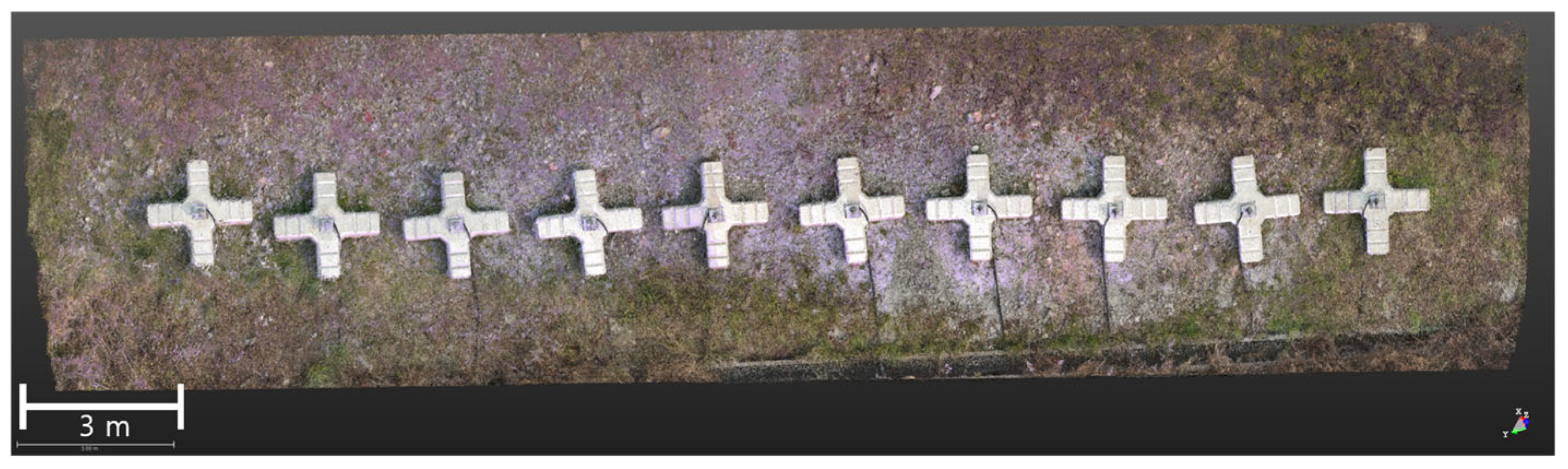
4.1. Experimental Area
4.2. UAS Data
4.3. TLS Data
4.4. Create a Combination Model
4.5. Accuracy and Reproducibility Review
5. Results and Discussion
5.1. Detection of Damage Factor
5.2. Crack Analysis
5.3. Analysis of Destruction
5.4. Analysis of Ground Adhesion
5.5. Analysis of Rotational Displacement
5.6. Discussion
6. Conclusions
- In vertical structures, such as slopes, the z-coordinate error of the 3D numerical model based on UAS images was relatively larger than the x- and y-coordinate errors. This issue is particularly pronounced in uneven structures with installed anchors, where data gaps arise owing to blind spots caused by the photographic angle. To address this problem, a 3D numerical model was created by combining TLS scan data. This model improved the accuracy of the z-coordinate through the mutual complementation of the two datasets;
- By constructing a 3D numerical model, the accuracy difference due to resolution was assessed for crack detection. In the 3D numerical model with 8 K resolution, cracks smaller than 0.3 mm were detected with an error range of ±0.05 mm. This led to important findings regarding maintenance;
- The 3D model achieved an approximate reproduction accuracy of 95%. However, distortion in the anchors installed on slopes, caused by factors such as vegetation and gravel, resulted in an error ranging from 6.2% to 17.1% compared with the designed area. Additional research is required to address these interfering factors;
- Numerical values for area and volume of failures were detected, with the failure area of the anchor water pressure plate ranging from 0.29% to 3.93% compared with the design, indicating minor damage. Although squantitative evaluation metrics for anchor failure have not yet been established, accumulating numerical data from 3D numerical models could provide a basis for quantitative maintenance evaluations;
- For important anchors where z-coordinate data are crucial, ground adhesion detection was not possible with the UAS 3D numerical model owing to the low overlap from a low shooting angle and blind spots from uneven structures. However, the combined analysis with TLS point cloud data enabled the measurements of ground elevation differences. Ground subsidence was 0.081 m at anchor 7 and 0.126 m at anchor 10. Rotational displacement of the anchor head was observed at anchors 2, 5, 6, and 7, with fine rotation angles measurable within 1°;
- This study confirmed that image-based 3D numerical models offer considerable potential for area analysis, such as crack and failure detection. However, for damage assessment involving displacement and ground subsidence, TLS point cloud data provides higher accuracy and precision compared with images. Therefore, the combination of UAS and TLS data to create a 3D numerical model was validated, showcasing the advantages of each method while addressing their respective limitations.
Author Contributions
Funding
Data Availability Statement
Conflicts of Interest
Abbreviations
| UAS | Utilized unmanned aerial systems |
| TLS | Terrestrial laser scanners |
| LiDAR | Light detection and ranging |
| GNSS | Global navigation satellite systems |
| GCP | Ground control points |
| BIM | Building information modeling |
| SfM | Structure from motion |
| ICP | Iterative closest point |
| SiamGCN | Siamese graph convolutional networks |
| KPConv | Kernel point convolution |
| TBM | Temporary bench marks |
| SCP | Scan control points |
| VCP | Vertical control points |
| VRS | Virtual reference station |
| RMS | Root-mean-square |
| CMR+ | Compact measurement record + |
| CMRx | Compact measurement record x |
| RTCM | Radio technical commision for maritime services |
| NVEA | National marine electronics association |
| FOV | Field of view |
| TIN | Triangulated irregular networks |
| STD | Standard deviation |
| RMSE | Root-mean-square error |
| GSD | Ground sampling distance |
References
- Moon, J.Y.; Kim, K.Y.; Choi, Y.U.; Min, S.J. The characteristics of Changma rainfall in South Korea during the new climatological period of 1991–2020. J. Clim. Res. 2020, 15, 139–152. [Google Scholar] [CrossRef]
- Kwon, O.I. Slope investigation, inspection and maintenance advanced technology based on digital infrastructure information. J. Korean Geosynth. Soc. 2021, 20, 8–16. [Google Scholar]
- Ministry of Public Safety and Security. The 2020 Annual Natural Disaster Report; Ministry of Public Safety and Security: Beijing, China, 2020. [Google Scholar]
- Lee, Y.C.; Kang, J.O. The precise three dimensional phenomenon modeling of the cultural heritage based on UAS imagery. J. Cadastre Land. Inf. 2019, 49, 85–101. [Google Scholar]
- Webb, R.H.; Boyer, D.E.; Turner, R.M. Repeat Photography: Methods and Applications in the Natural Sciences; Island Press: Washington, DC, USA, 2010; p. 337. Available online: https://www.researchgate.net/publication/265780270_Repeat_Photography_Methods_and_Applications_in_the_Natural_Sciences (accessed on 1 March 2025).
- Amaury, F.; Nyssen, J.; De Dapper, M.; Haile, M.; Billi, R.P.; Munro, N.; Deckers, J.; Poesen, J. Linking long-term gully and river channel dynamics to environmental change using repeat photography (Northern Ethiopia). Geomorphology 2011, 129, 238–251. [Google Scholar] [CrossRef]
- Wheaton, J.M.; Brasington, J.; Darby, S.E.; Sear, D.A. Accounting for uncertainty in DEMs from repeat topographic surveys: Improved sediment budgets. Earth Surf. Process. Landf. 2010, 35, 136–156. [Google Scholar] [CrossRef]
- Liu, P.; Chen, A.Y.; Huang, Y.-N.; Han, J.-Y.; Lai, J.-S.; Kang, S.-C.; Wu, T.-H.; Wen, M.-C.; Tsai, M.-H. A review of rotorcraft unmanned aerial vehicle (UAV) developments and applications in civil engineering. Smart Struct. Syst. 2014, 13, 1065–1094. [Google Scholar] [CrossRef]
- Brodu, N.; Lague, D. 3D terrestrial lidar data classification of complex natural scenes using a multi-scale dimensionality criterion: Applications in geomorpholog. ISPRS J. Photogramm. Remote Sens. 2012, 68, 121–134. [Google Scholar] [CrossRef]
- Waldemar, K.; Kubisz, W.; Zagórski, P. Use of terrestrial laser scanning (TLS) for monitoring and modelling of geomorphic processes and phenomena at a small and medium spatial scale in polar environment (Scott River—Spitsbergen). Geomorphology 2014, 212, 84–96. [Google Scholar] [CrossRef]
- Xiao, Y.; Wang, C.; Li, J.; Zhang, W.; Xi, X.; Wang, C.; Dong, P. Building segmentation and modeling from airborne LiDAR data. Int. J. Digit. Earth 2015, 8, 694–709. [Google Scholar] [CrossRef]
- Cho, H.K.; Jang, K.T.; Hong, S.J.; Hong, G.P.; Kim, S.H.; Kwon, S.H. Accuracy analysis for slope movement characterization by comparing the data from real-time measurement device and 3D model value with drone based photogrammetry. J. Korean Assoc. Geogr. Inf. Stud. 2020, 23, 234–252. [Google Scholar]
- Kang, I.; Kim, T. Accuracy evaluation of 3D slope model produced by drone taken images. J. Korean GEO-Environ. Soc. 2020, 21, 13–17. [Google Scholar] [CrossRef]
- Pingbo, T.; Huber, D.; Akinci, B.; Lipman, R.; Lytle, A. Automatic reconstruction of as-built building information models from laser-scanned point clouds: A review of related techniques. Autom. Constr. 2010, 19, 829–843. [Google Scholar] [CrossRef]
- Hong, S.K.; Park, H.J. Probabilistic kinematic analysis of rook slope stability using terrestrial LiDAR. Econ. Environ. Geol. 2019, 52, 231–241. [Google Scholar] [CrossRef]
- Hellmy, A.; Muhammad, R.F.; Ng, T.F.; Abdullah, W.; Shuib, M. Rock Slope Stability Analysis based on Terrestrial LiDAR on Karst Hills in Kinta Valley Geopark, Perak, Peninsular Malaysia. Sains Malays. 2019, 48, 2595–2604. [Google Scholar] [CrossRef]
- Park, J.-K. A study of monitoring in slopes of high collapse risk using terrestrial LiDAR. J. Korean Soc. Hazard. Mitig. 2010, 10, 45–52. [Google Scholar]
- Lee, K.W.; Park, J.K. Application of Terrestrial LiDAR for Displacement Detecting on Risk Slope. J. Korean Acad.-Ind. Coop. Soc. 2019, 20, 323–328. [Google Scholar] [CrossRef]
- Grenzdörffer, G.J.; Naumann, M.; Niemeyer, F.; Frank, A. Symbiosis of UAS photogrammetry and TLS for surveying and 3D modeling of cultural heritage monuments—A case study about the cathedral of St. Nicholas in the city of Greifswald. Int. Arch. Photogramm. Remote Sens. Spat. Inf. Sci. 2015, 40, 91–96. [Google Scholar] [CrossRef]
- Subiyanto, S.; Bashit, N.; Rianty, N.D.; Savitri, A.D. Combination of terrestrial laser scanner and unmanned aerial vehicle technology in the manufacture of building information model. J. Appl. Geospat. Inf. 2021, 5, 520–525. [Google Scholar] [CrossRef]
- Kim, S.; DaJinSol, K.; Yoon, S.D.; Ju, N.H. Assessment and analysis of disaster risk for steep slope using drone and terrestrial LiDAR. J. Korean Soc. Geospat. Inf. Sci. 2020, 28, 13–24. [Google Scholar] [CrossRef]
- Kang, J.O.; Lee, Y.C. Construction of 3D spatial information of vertical structure by combining UAS and terrestrial LiDAR. J. Cadastre Land. Inf. 2019, 49, 57–66. [Google Scholar] [CrossRef]
- Besl, P.J.; McKay, N.D. A method for registration of 3-D shapes. IEEE Trans. Pattern Anal. Mach. Intell. 1992, 14, 239–256. [Google Scholar] [CrossRef]
- Chen, Y.; Medioni, G. Object Modeling by Registration of Multiple Range Images. IEEE Int. Conf. Robot. Autom. 1992, 10, 145–155. [Google Scholar] [CrossRef]
- Glira, P.; Pfeifer, N.; Briese, C.; ReSSl, C. A correspondence framework for ALS strip adjustments based on variants of the ICP algorithm. Photogramm. Fernerkund. Geoinf. 2015, 4, 275–289. [Google Scholar] [CrossRef]
- OPALS—Orientation and Processing of Airborne Laser Scanning Data. Available online: https://opals.geo.tuwien.ac.at/html/stable/ModuleICP.html (accessed on 24 August 2024).
- Rusinkiewicz, S.; Levoy, M. Efficient Variants of the ICP Algorithm. In Proceedings of the Third International Conference on 3-D Digital Imaging and Modeling (3DIM), Quebec City, QC, Canada, 8 May–1 June 2001; pp. 145–152. [Google Scholar] [CrossRef]
- Lee, Y.C.; Cho, E.S.; Kang, J.O. Analysis of the effectiveness of UAS smart sensor-based rock slope safety diagnosis. J. Korean Soc. Surv. Geod. Photogramm. Cartogr. 2024, 42, 137–148. [Google Scholar] [CrossRef]
- Rongjun, Q.; Tian, J.; Reinartz, P. 3D change detection–Approaches and applications. ISPRS J. Photogramm. Remote Sens. 2016, 122, 41–56. [Google Scholar] [CrossRef]
- Neuner, H.; Holst, C.; Kuhlmann, H. Overview on current modelling strategies of point clouds for deformation analysis. Allg. Vermess.-Nachrichten 2016, 123, 328–339. Available online: https://portal.fis.tum.de/en/publications/overview-on-current-modelling-strategies-of-point-clouds-for-defo (accessed on 3 March 2025).
- Wunderlich, T.; Niemeier, W.; Wujanz, D.; Holst, C.; Neitzel, F.; Kuhlmann, H. Areal deformation analysis from TLS point clouds–The challenge. Allg. Vermess.-Nachrichten 2016, 123, 340–351. Available online: https://www.researchgate.net/publication/311795322_Areal_Deformation_Analysis_from_TLS_Point_Clouds_-_The_Challenge (accessed on 3 March 2025).
- Harmening, C.; Hobmaier, C.; Neuner, H. Laser scanner–based deformation analysis using approximating B-spline surfaces. Remote Sens. 2021, 13, 3551. [Google Scholar] [CrossRef]
- Cignoni, P.; Rocchini, C.; Scopigno, R. Metro: Measuring error on simplified surfaces. Comput. Graphics Forum 1998, 17, 167–174. [Google Scholar] [CrossRef]
- Aspert, N.; Santa-Cruz, D.; Ebrahimi, T. MESH: Measuring Errors Between Surfaces Using the Hausdorff Distance. In Proceedings of the IEEE International Conference on Multimedia and Expo, ICME 2002, Lausanne, Switzerland, 26–29 August 2002; pp. 705–708. [Google Scholar] [CrossRef]
- Gojcic, Z.; Zhou, C.; Wieser, A. F2S3: Robustified determination of 3D displacement vector fields using deep learning. J. Appl. Geodesy 2020, 14, 177–189. [Google Scholar] [CrossRef]
- Zahs, V.; Winiwarter, L.; Anders, K.; Williams, J.G.; Rutzinger, M.; Höfle, B. Correspondence-driven plane-based M3C2 for lower uncertainty in 3D topographic change quantification. ISPRS J. Photogramm. Remote Sens. 2022, 183, 541–559. [Google Scholar] [CrossRef]
- Travelletti, J.; Malet, J.-P.; Delacourt, C. Image-based correlation of laser scanning point cloud time series for landslide monitoring. Int. J. Appl. Earth Obs. Geoinf. 2014, 32, 1–18. [Google Scholar] [CrossRef]
- Holst, C.; Janßen, J.; Schmitz, B.; Blome, M.; Dercks, M.; Schoch-Baumann, A.; Blöthe, J.; Schrott, L.; Kuhlmann, H.; Medic, T. Increasing spatio-temporal resolution for monitoring alpine solifluction using terrestrial laser scanners and 3D vector fields. Remote Sens. 2021, 13, 1192. [Google Scholar] [CrossRef]
- Yang, Y.; Balangé, L.; Gericke, O.; Schmeer, D.; Zhang, L.; Sobek, W.; Schwieger, V. Monitoring of the production process of graded concrete component using terrestrial laser scanning. Remote Sens. 2021, 13, 1622. [Google Scholar] [CrossRef]
- Lane, S.N.; Westaway, R.M.; Hicks, D.M. Estimation of erosion and deposition volumes in a large, gravel-bed, braided river using synoptic remote sensing. Earth Surf. Process Landf. 2003, 28, 249–271. [Google Scholar] [CrossRef]
- Lague, D.; Brodu, N.; Leroux, J. Accurate 3D comparison of complex topography with terrestrial laser scanner: Application to the Rangitikei Canyon (N-Z). ISPRS J. Photogramm. Remote Sens. 2013, 82, 10–26. [Google Scholar] [CrossRef]
- Winiwarter, L.; Anders, K.; Höfle, B. M3C2-EP: Pushing the limits of 3D topographic point cloud change detection by error propagation. ISPRS J. Photogramm. Remote Sens. 2021, 178, 240–258. [Google Scholar] [CrossRef]
- Teza, G.; Galgaro, A.; Zaltron, N.; Genevois, R. Terrestrial laser scanner to detect landslide displacement fields: A new approach. Int. J. Remote Sens. 2007, 28, 3425–3446. [Google Scholar] [CrossRef]
- de Gélis, I.; Lefèvre, S.; Corpetti, T. Siamese KPConv: 3D multiple change detection from raw point clouds using deep learning. ISPRS J. Photogramm. Remote Sens. 2023, 197, 274–291. [Google Scholar] [CrossRef]
- Al-jibury, E.; King, J.W.D.; Guo, Y.; Lenhard, B.; Fisher, A.G.; Merkenschlager, M.; Rueckert, D. A deep learning method for replicate-based analysis of chromosome conformation contacts using siamese neural networks. Nat. Commun. 2023, 14, 5007. [Google Scholar] [CrossRef]
- Dewez, T.J.B.; Girardeau-Montaut, D.; Allanic, C.; Rohmer, J. Facets: A cloudcompare plug in to extract geological planes from unstructured 3D point clouds. Int. Arch. Photogramm. Remote Sens. Spat. Inf. Sci. 2016, 41, 799–804. [Google Scholar] [CrossRef]
- Shigeta, Y.; Maeda, K.; Yamamoto, H.; Yasuda, T.; Kaise, S.; Maegawa, K.; Ito, T. Tunnel deformation evaluation by mobile mapping system. In Tunnels and Underground Cities: Engineering and Innovation Meet Archaeology, Architecture and Art, 1st ed.; CRC Press: London, UK, 2019; pp. 3097–3104. [Google Scholar]
- Wang, H.; Wang, Q.; Zhai, J.; Yuan, D.; Zhang, W.; Xie, X.; Zhou, B.; Cai, J.; Lei, Y. Design of fast acquisition system and analysis of geometric feature for highway tunnel lining cracks based on machine vision. Appl. Sci. 2022, 12, 2516. [Google Scholar] [CrossRef]


| Trimble R8 | Parameters | |||
|---|---|---|---|---|
 | weight | 1.52 kg | channel | 440 channels |
| stop positioning vertical | 3.5 mm + 0.4 parts per million (ppm) root-mean-square (RMS) | input | CMR+, CMRx, RTCM2.1–3.1 | |
| stop positioning horizontal | 3 mm + 0.1 ppm RMS | output | 16 NMEA | |
| RTK vertical | 20 mm + 1 ppm RMS | radio modem | 450 MHz | |
| RTK horizontal | 10 mm + 1 ppm RMS | signal update cycle | 1–20 Hz | |
| HTS-420R | Parameters | |
|---|---|---|
 | weight | 5.5 kg |
| accuracy | 0.00001 rad | |
| minimum focusing distance | 1.5 m | |
| prism mode | ±(2 mm + 2 ppm) | |
| reflectorless | ±(3 mm + 2 ppm) | |
| Test | A (TLS) | B (UAS) | C (Combined UAS and TLS) | |
|---|---|---|---|---|
| X | maximum (MAX) | 30 | 28 | 30 |
| minimum (MIN) | 0 | 0 | 0 | |
| average (AVG) | 8 | 12 | 5 | |
| Y | MAX | 30 | 28 | 30 |
| MIN | 1 | 0 | 0 | |
| AVG | 14 | 14 | 9 | |
| XY | MAX | 30 | 30 | 29 |
| MIN | 1 | 3 | 1 | |
| AVG | 17 | 18 | 11 | |
| STD | 8 | 8 | 7 | |
| RMSE | 19 | 19 | 13 | |
| Z | MAX | 22 | 50 | 32 |
| MIN | 0 | 7 | 0 | |
| AVG | 8 | 36 | 6 | |
| STD | 4 | 12 | 4 | |
| RMSE | 9 | 38 | 7 | |
| (Unit: mm) | ||||
| No. | Marking Damage Factor | No. | Marking Damage Factor |
|---|---|---|---|
| 1 |  | 2 |  |
| 3 |  | 4 |  |
| 5 |  | 6 |  |
| 7 | 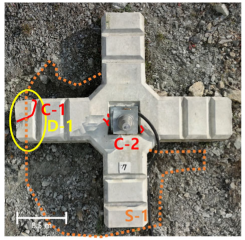 | 8 |  |
| 9 | 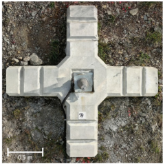 | 10 | 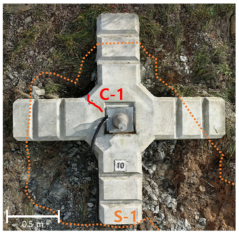 |
| No. | Field Measurement | 3D Model | Error |
|---|---|---|---|
| 3-C3-1 |  | 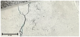 | 0.05 |
| 0.75 | 0.80 | ||
| 3-C3-3 |  | 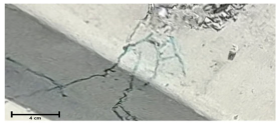 | 0.03 |
| 0.50 | 0.53 | ||
| 3-C3-2 | 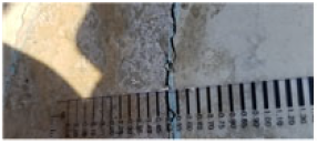 |  | 0.04 |
| 0.50 | 0.54 | ||
| 4-C1-1 | 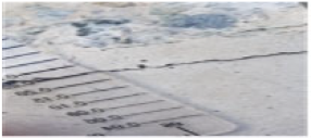 | 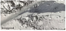 | 0.03 |
| 0.25 | 0.28 | ||
| 4-C2-1 | 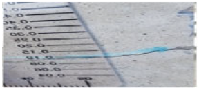 | 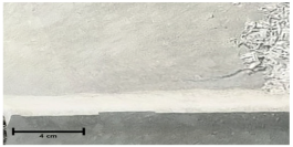 | 0.11 |
| 0.10 | 0.21 | ||
| 7-C1-1 | 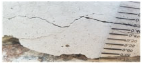 |  | 0.03 |
| 0.35 | 0.38 | ||
| 8-C2-1 | 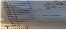 | 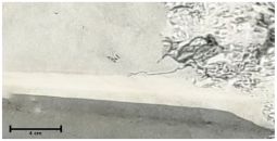 | 0.03 |
| 0.20 | 0.23 | ||
| 8-C1-1 |  |  | 0.05 |
| 0.45 | 0.50 | ||
| (Unit: mm) | |||
| Anchor No. | 3D Model (4 K) | 3D Model (8 K) | Measurements |
|---|---|---|---|
| 3 | 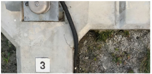 | 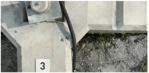 | field: 0.15 4 K: −0.18 8 K: −0.06 |
| 0.33 | 0.21 | ||
| 7 |  |  | field: 0.30 4 K: −0.21 8 K: 0.0 |
| 0.51 | 0.30 | ||
| (Unit: mm) | |||
| Anchor No. | Design Surface Area | Surface Area of 3D Model | Measured Efficiency | Failure Area | Percentage of Failure |
|---|---|---|---|---|---|
| 1 | 3.736 m2 | 3.476 m2 | 6.9% | - | - |
| 2 | 3.115 m2 | 16.6% | 0.011 m2 | 0.29% | |
| 3 | 3.156 m2 | 15.5% | 0.147 m2 | 3.93% | |
| 4 | 3.100 m2 | 17.0% | 0.098 m2 | 2.62% | |
| 5 | 3.098 m2 | 17.1% | - | - | |
| 6 | 3.181 m2 | 14.9% | 0.107 m2 | 2.86% | |
| 7 | 3.349 m2 | 10.4% | 0.050 m2 | 1.34% | |
| 8 | 3.504 m2 | 6.2% | 0.083 m2 | 2.22% | |
| 9 | 3.121 m2 | 16.5% | - | - | |
| 10 | 3.382 m2 | 9.5% | - | - |
| Anchor No. | Photograph | 3D Model |
|---|---|---|
| 3 | 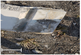 | 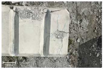 |
| 2 |  |  |
| Anchor No. | Designed Volume | Failure Volume | Total | |||
|---|---|---|---|---|---|---|
| B1 | B2 | B3 | B4 | |||
| 2 | 538,973 | 130.16 | - | - | - | 130.16 |
| 3 | 1792.84 | 21.11 | 264.53 | 108.52 | 2187.00 | |
| 4 | 1258.10 | 25.84 | 261.84 | - | 1545.78 | |
| 6 | 2256.20 | 32.49 | - | - | 2288.69 | |
| 7 | 1812.69 | - | - | - | 1812.69 | |
| 8 | 2125.00 | 1488.98 | - | - | 3613.98 | |
| (Unit: cm3) | ||||||
| Anchor No. | Detected Points | Settlement | ||
|---|---|---|---|---|
| 1 |  | A | B | C |
| 0.007 | 0.017 | 0.004 | ||
| D | E | |||
| 0.024 | - | 0.018 | ||
| F | G | H | ||
| 0.034 | 0.017 | 0.014 | ||
| 7 |  | A | B | C |
| 0.064 | 0.018 | 0.028 | ||
| D | E | |||
| 0.044 | - | 0.024 | ||
| F | G | H | ||
| 0.155 | 0.040 | 0.119 | ||
| 10 |  | A | B | C |
| 0.013 | 0.009 | 0.027 | ||
| D | E | |||
| 0.011 | - | 0.014 | ||
| F | G | H | ||
| 0.179 | 0.018 | 0.152 | ||
| (Unit: m) | ||||
| Anchor No. | Detection of 20 Settlement Points | Average Settlement |
|---|---|---|
| 7 |  | 0.081 |
| 10 |  | 0.126 |
| (unit: m) | ||
| Anchor No. | Before Damage | After Damage | Rotational Displacement | |
|---|---|---|---|---|
| 2 |  |  |  | Rotation angle =1.31° Displacement = 0.005 m |
| 5 | 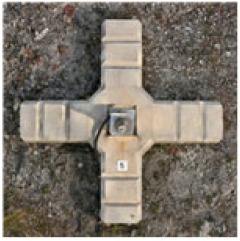 | 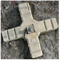 | 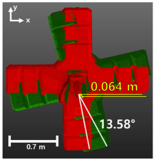 | Rotation angle = 13.58° Displacement = 0.064 m |
| 6 | 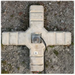 |  | 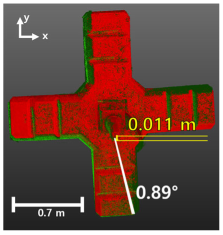 | Rotation angle = 0.89° Displacement = 0.011 m |
| 7 |  | 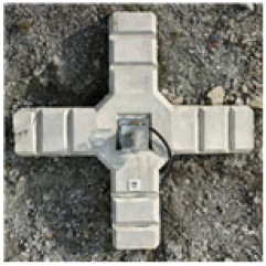 | 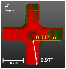 | Rotation angle = 0.97° Displacement = 0.042 m |
Disclaimer/Publisher’s Note: The statements, opinions and data contained in all publications are solely those of the individual author(s) and contributor(s) and not of MDPI and/or the editor(s). MDPI and/or the editor(s) disclaim responsibility for any injury to people or property resulting from any ideas, methods, instructions or products referred to in the content. |
© 2025 by the authors. Licensee MDPI, Basel, Switzerland. This article is an open access article distributed under the terms and conditions of the Creative Commons Attribution (CC BY) license (https://creativecommons.org/licenses/by/4.0/).
Share and Cite
Lee, C.; Kang, J. Case Study on the Use of an Unmanned Aerial System and Terrestrial Laser Scanner Combination Analysis Based on Slope Anchor Damage Factors. Remote Sens. 2025, 17, 1400. https://doi.org/10.3390/rs17081400
Lee C, Kang J. Case Study on the Use of an Unmanned Aerial System and Terrestrial Laser Scanner Combination Analysis Based on Slope Anchor Damage Factors. Remote Sensing. 2025; 17(8):1400. https://doi.org/10.3390/rs17081400
Chicago/Turabian StyleLee, Chulhee, and Joonoh Kang. 2025. "Case Study on the Use of an Unmanned Aerial System and Terrestrial Laser Scanner Combination Analysis Based on Slope Anchor Damage Factors" Remote Sensing 17, no. 8: 1400. https://doi.org/10.3390/rs17081400
APA StyleLee, C., & Kang, J. (2025). Case Study on the Use of an Unmanned Aerial System and Terrestrial Laser Scanner Combination Analysis Based on Slope Anchor Damage Factors. Remote Sensing, 17(8), 1400. https://doi.org/10.3390/rs17081400