1. Introduction
With the rapid advancement of machine learning, its application in atmospheric science has expanded significantly [
1,
2,
3]. Machine learning has become a powerful tool for analyzing and predicting complex atmospheric processes that traditional methods struggle to model. These techniques have improved our ability to understand and forecast dynamic atmospheric phenomena, particularly within the atmospheric boundary layer (ABL) [
4,
5,
6]. The ABL plays a critical role in the Earth’s climate system through the exchange of momentum, heat, and moisture between the surface and the free atmosphere [
7,
8]. These exchanges in ABL directly affect the hydrological cycle, radiation balance, weather patterns, climate dynamics, and air quality. Accurate characterizing the ABL is essential for various applications, including weather forecasting, climate modeling, and pollution control [
9,
10,
11]. However, predicting ABL behavior remains challenging due to its complexity from sensitivity to surface conditions and interactions with the broader atmosphere [
8,
10].
Recent advancements in machine learning have led to the development of new methods for addressing these challenges in atmospheric science studies. Models such as XGBoost and neural networks have proven effective in analyzing the impacts of meteorological parameters on the mixing layer height (MLH), a key indicator of ABL evolution [
12,
13,
14]. These models are well-suited for handling large datasets and capturing complex, nonlinear relationships, making them effective tools for studying ABL processes. Despite these successes, most studies have relied on single field experiments or annual datasets from specific sites [
15,
16,
17]. While these studies provide useful insights, they often overlook significant seasonal variations in ABL dynamics. It is well established that factors influencing the ABL vary by season due to changes in solar radiation, surface heating, and atmospheric stability [
18,
19,
20].
To capture seasonal variations accurately, data need to be segmented by season. However, this approach reduces the dataset size, which may compromise the reliability of results [
21,
22]. Atmospheric observations are costly and logistically complex, limiting the availability of long-term, high-quality datasets. As a result, obtaining sufficient data for detailed seasonal analysis is challenging [
11,
23,
24,
25,
26]. Extending the observation period can help increase the dataset size. However, it may introduce systematic errors due to instrument aging, changes in detection models, or component replacements, all of which affect data consistency [
27,
28]. Thus, more data do not always lead to better results. The difficulty of long-term data collection and consistency issues further complicate the issue. Researchers continue to explore ways to maximize the effectiveness of limited datasets.
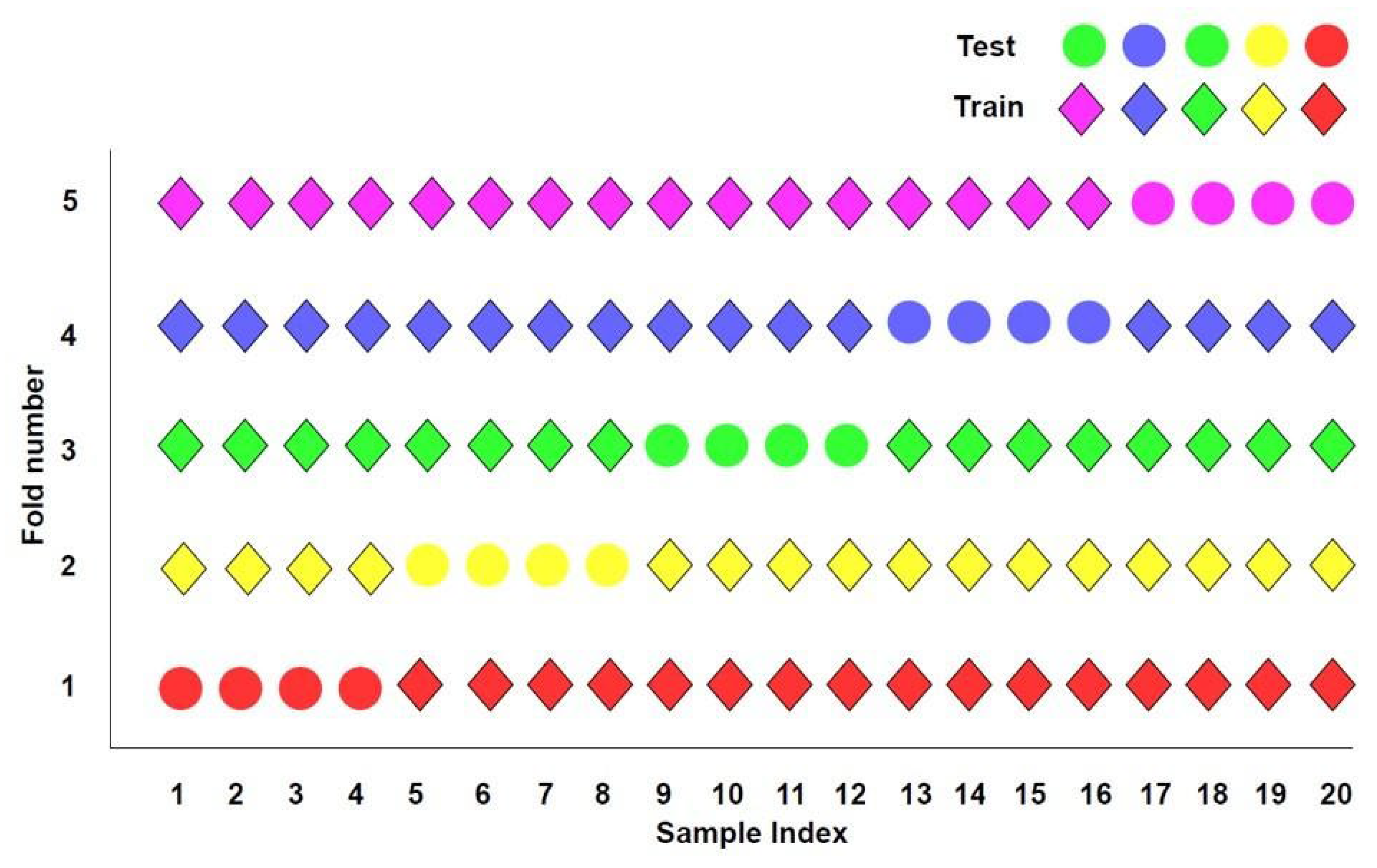
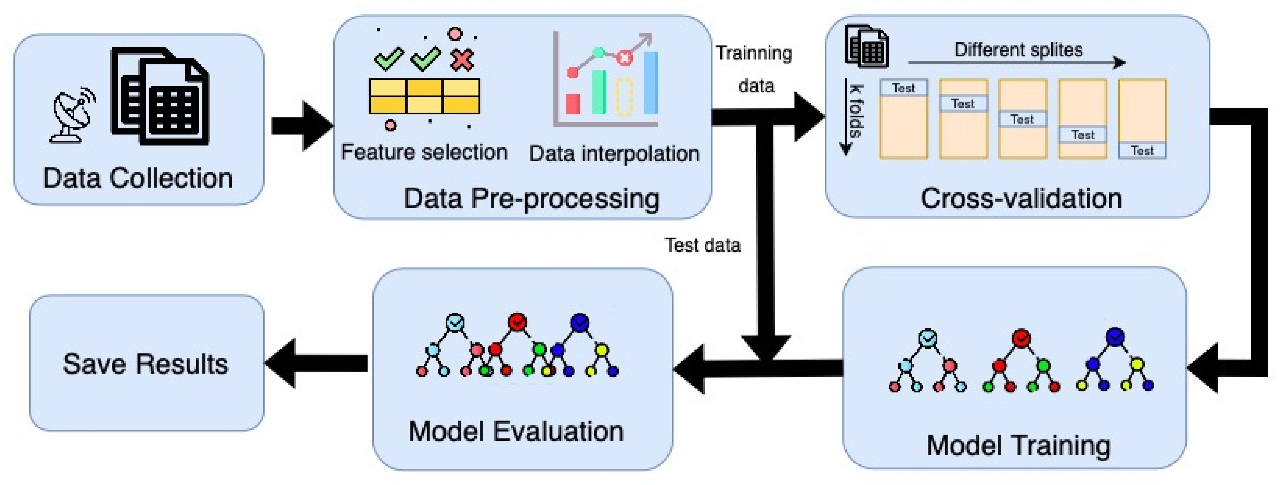
To address these challenges, our study aims to integrate cross-validation with extreme gradient boosting (XGBoost) to analyze the seasonal impacts. Cross-validation is a robust statistical technique that enhances model reliability by partitioning the dataset into multiple folds, ensuring that the model is trained and tested on different subsets. Grid search optimization identifies the optimal parameter settings for the dataset, reducing errors associated with default parameters. This approach maximizes the use of available data and mitigates the risk of overfitting, thereby improving the generalizability of the results [
29,
30,
31,
32]. Building on this foundation, our study aims to provide a more refined understanding of seasonal variations in the factors influencing MLH, offering valuable insights into future atmospheric research and modeling.
Numerous meteorological factors influence ABL development, leading many studies to use dozens of input parameters. Excessive data can increase measurement errors, and if boundary layer variations can be simulated using the fewest possible parameters, these errors can be minimized. To quantify and distinguish the varying degrees of influence among these input parameters, we introduce the concept of ‘relative importance’, which serves as a metric to assess their contributions to the model’s predictive performance. Based on the boundary layer theory, both thermodynamic forcing (through buoyancy production) and shear production are key drivers of turbulence, with their relative contributions varying depending on conditions [
7,
10]. To capture seasonal variations in key influencing factors, this study adopts a streamlined approach by selecting sensible heat flux (SHF), latent heat flux (LHF), and lower tropospheric stability (LTS) as input variables, with the mixed layer height (MLH) as the output. This selection is guided by the boundary layer theory, where thermodynamic processes and heat flux contributions provide a physical constraint for estimating CBLH. Specifically, these parameters reflect the atmospheric heat absorption and stability dynamics that govern boundary layer development, as opposed to relying on numerous parameters without such constraints [
7,
10]. Additionally, our study applies cross-validation to analyze multi-year lidar data from the atmospheric radiation measurement (ARM) Southern Great Plains (SGP) site [
13,
33,
34].
Therefore, this study focuses on heat fluxes (SHF, LHF) and LTS, utilizing the XGBoost algorithm to predict MLH and analyze the relative contributions of these factors. The structure of this paper is as follows:
Section 2 introduces the dataset used, along with the cross-validation and XGBoost methods.
Section 3 validates the consistency of the results obtained using the XGBoost method alone and the combined approach of cross-validation and XGBoost.
Section 4 investigates the influence of various factors on the mixed layer height (MLH) at the four ARM Southern Great Plains (SGP) sites (C1, E32, E37, E79) across different seasons, employing a combination of cross-validation and the XGBoost method. Subsequently, we compare the relative influence factors and their variations at different times of day across seasons, further informed by analyses of wind direction and SHAP value. Finally, this paper concludes with a conclusion.
3. Validation of the Two Methods Using the ARM Site Dataset
3.1. Impact of Different Parameter Settings on the Results of the XGBoost Algorithm
To examine the impact of different XGBoost parameters on the results, we tested various parameter combinations, as shown in
Table 2. The range of n_estimators is 50–400, learning_rate varies from 0.01 to 0.5, and max_depth ranges from 3 to 9. In
Table 2, the leftmost column, labeled “Group”, represents comparisons where only one parameter is adjusted while the others remain constant. Groups 1–3 compare the effects of n_estimators, learning_rate, and max_depth, respectively. Groups 4 and 5 involve manual tuning to identify the optimal parameter combination.
From Group 1, we observe that the correlation coefficient R2 increases as the number of estimators (n_estimators) increases. In this case, learning_rate and max_depth are fixed at 0.1 and 3, respectively. As the n_estimators parameter increases from 50 to 300, R improves from 0.60 to 0.73. Additionally, LTS decreases while SHF and LHF increase as the n_estimators parameter increases. Although a higher n_estimators parameter improves R, considering that the number of sampling days in this study is under 1000, setting n_estimators too high is not recommended. To balance performance and computational efficiency, it should remain below 200.
Group 2 shows that the correlation coefficient R2 increases as the learning_rate rises. In this case, n_estimators and max_depth are fixed at 100 and 3, respectively. As learning_rate increases from 0.01 to 0.5, R2 improves from 0.48 to 0.78. This trend is expected, as R2 is the lowest (0.48) when learning_rate is set to 0.01. Additionally, as learning_rate increases, the relative influence of LTS decreases, while SHF and LHF gain more importance. Since our sample size is under 1000, we do not recommend using a very low learning_rate. To maintain model efficiency and accuracy, it should be kept above 0.1.
Group 3 demonstrates that the correlation coefficient R2 increases as max_depth increases. In this case, n_estimators and learning_rate are fixed at 200 and 0.3, respectively. As max_depth increases from 3 to 9, R improves from 0.79 to 0.84. However, the change in R becomes minimal (less than 0.05) when max_depth increases from 5 to 9. Similarly, the relative influence of LTS, SHF, and LHF shows only slight variations. Since our sample size is under 1000, we do not recommend setting max_depth too high. To balance performance and computational efficiency, it should be kept below 7.
The objective of Group 4 is to evaluate the impact of varying other parameters while keeping max_depth fixed at 5. The results show that when n_estimators is set to 400, the difference in R2 between the learning_rate values of 0.1 and 0.5 is less than 0.01. However, when n_estimators is set to 100, the change in R2 between the same learning_rate values is slightly larger, at less than 0.08. Additionally, the difference in R2 between the parameter combinations (n_estimators, learning_rate) = (400, 0.1) and (100, 0.5) is also less than 0.01. This indicates that the relationship between R2 and these parameters is not strictly linear, and different parameter combinations can yield similar results. However, while R values may be comparable, slight differences remain in the relative influence of LTS, SHF, and LHF.
Group 5 builds on Group 4 by varying the max depth, further confirming that the relationship between the correlation coefficient R2 and the parameters is not linear, and different combinations can produce similar results. Therefore, it is necessary to carefully select XGBoost hyperparameters rather than simply using the default settings.
3.2. Impact of Different Cross-Validation Parameter Settings on the Results of the XGBoost Algorithm
The results in
Section 3.1 indicate that different XGBoost parameters significantly affect the outcomes. The default hyperparameters are typically set as ‘n_estimators’: [50, 100, 200], ‘learning_rate’: [0.01, 0.1, 0.2], and ‘max_depth’: [3, 5, 7]. The results obtained using these default parameters are shown in
Table 3 under ‘Default Parameters’. The results show that although the value of R does not change significantly (less than 0.01) as N splits vary from 3 to 12, the R
2 value remains around 0.6. Further analysis revealed that although we set ‘learning_rate’, i.e., [0.01, 0.1, 0.2], and ‘max_depth’, i.e., [3, 5, 7], the learning rate actually selected was 0.01. This is because the software tends to select a smaller learning rate by default to prevent overfitting. However, due to the limited sample size in this study, a smaller learning rate may prevent finding the optimal solution. Additionally, to prevent overfitting, the number of estimators (n_estimators) should not be set too high, so we need to set a larger learning rate. Moreover, the relationship between MLH (mixing layer height) and LTS, SHF, and LHF is a complex nonlinear relationship, so we also set the learning rate to be above 0.3.
The results obtained using the optimized hyperparameters are presented in
Table 3 under ‘Optimized Parameters’, showing improved performance. Based on the results from
Section 3.1 and the default parameters, and considering the specifics of this dataset, the hyperparameters were set as ‘n_estimators’: [50, 100, 200], ‘learning_rate’: [0.3, 0.5, 0.7], and ‘max_depth’: [5, 7, 9]. The results show that the R value is 0.83 when n_splits is 3, and it remains around 0.81 within the range of 3–15. Additionally, the relative influence factors for LTS, SHF, and LHF are 0.50, 0.28, and 0.22, respectively. This indicates that due to the small sample size, increasing the number of splits beyond a certain point does not affect the final averaged results.
The effect of different K values on the correlation coefficient R
2 is minimal; however, the impact on the relative importance of influencing factors is more pronounced. As illustrated in
Table 3, the R
2 values for K = 3 and K = 5 are 0.83 and 0.81, respectively, with a relative error of approximately ~0.02. In contrast, the variation in LHF can reach up to 0.09. This indicates that the choice of K values significantly influences the results, highlighting inconsistencies in performance across different datasets. Based on this evaluation, we determined that K = 3 provided the optimal performance among the tested values (3, 5, 7, 9, 12, 15) and, thus, it was consistently adopted in subsequent analyses, including
Section 4. A possible explanation for this could be the seasonal variation in the relative importance of influencing factors. However, a prerequisite for studying the relative importance of seasonal variations is that the model must be sufficiently accurate, meaning the correlation coefficient (R
2) should be adequately high, typically exceeding 0.8. Only when the model achieves such accuracy does the analysis of relative importance gain credibility.
4. Relative Influence Factors Across Different Seasons
To compare the relative influence factors of LTS, LHF, and SHF across different seasons, we applied the optimized parameters to the SGP sites. Since the dataset becomes smaller when divided by season, we now choose K = 3, as shown in the first row of
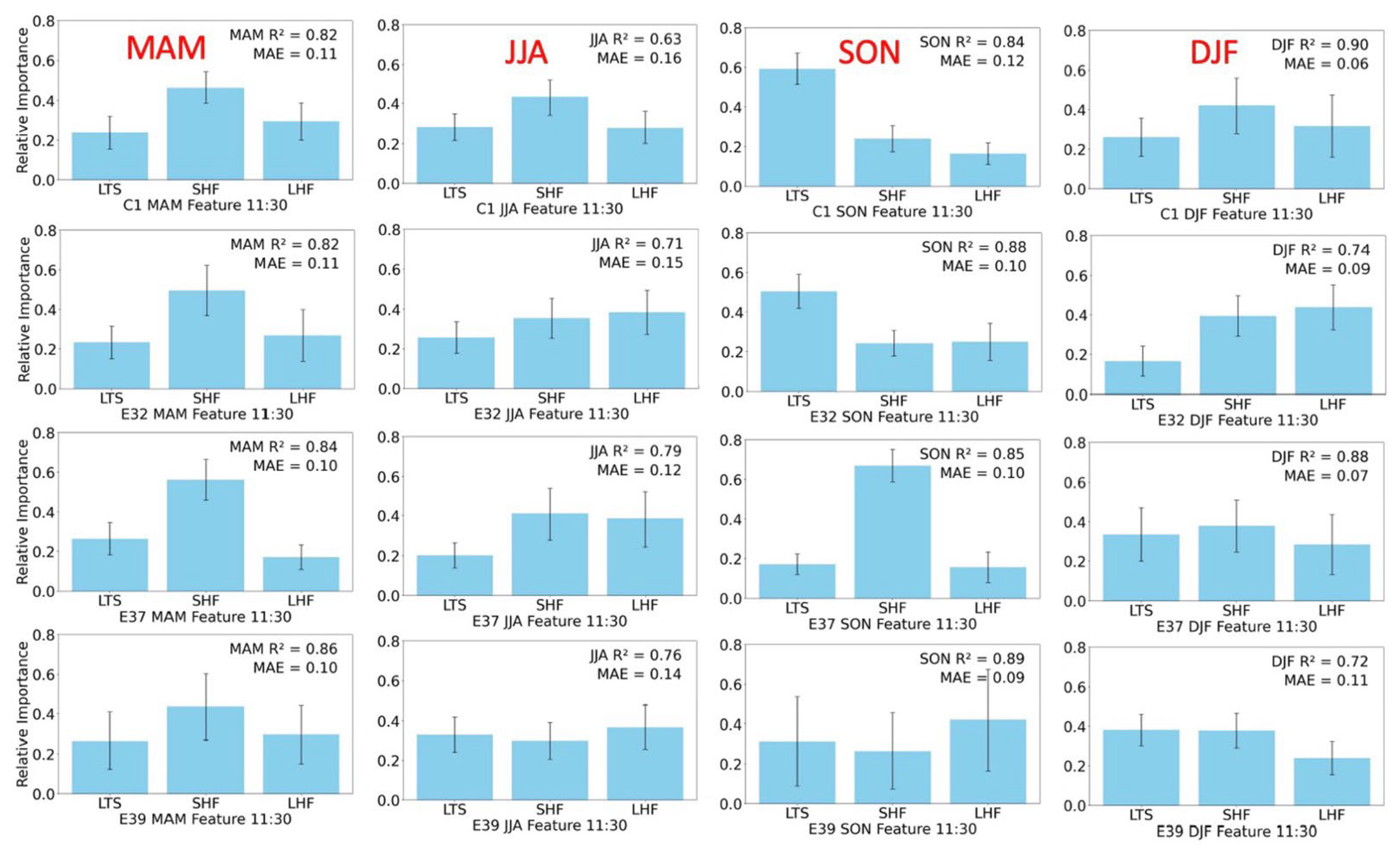
Figure 4. And the hyperparameters for individual seasons were set as follows: ‘n_estimators’: [50, 100, 200], ‘learning_rate’: [0.1, 0.3, 0.5], and ‘max_depth’: [3, 5, 7]. The dataset is divided into four seasons. DJF represents December, January, and February for winter; MAM represents March, April, and May for spring; JJA represents June, July, and August for summer; SON represents September, October, and November for autumn. To further compare the spatiotemporal variations across different sites and seasons, we combined and analyzed the seasonal data from C1, E32, E37, and E39, as presented in
Figure 4. The first row corresponds to the C1 site, the second row to the E32 site, the third row to the E37 site, and the fourth row to the E39 site. Additionally, the first column represents DJF (winter), the second column represents MAM (spring), the third column represents JJA (summer), and the last column represents SON (autumn).
The relative influence of key atmospheric factors varies significantly across seasons, deviating notably from the annual trends. At the C1 site, LTS dominates in SON, reaching a relative importance of 0.6, whereas in other seasons, SHF becomes the primary factor (MAM: 0.5, JJA: 0.42, DJF: 0.4). Since JJA and SON contain more data points compared to DJF, LTS appears as the dominant factor in the annual analysis with value approximately 0.5 (
Table 3). Additionally, during JJA, the relative contributions of LTS, SHF, and LHF are more balanced, with differences within 0.2, indicating a more equitable contribution of all three factors to ML development. In contrast, SON exhibits a more pronounced variation, with differences reaching up to 0.4, reinforcing the seasonal dependence of ML evolution. Comparing
Table 3, the annual correlation coefficient at C1 is 0.83, whereas the seasonal values in
Figure 4 are 0.90 for DJF, 0.82 for MAM, 0.84 for SON, and only 0.63 for JJA, indicating substantial seasonal variations. Although JJA contains more data points than MAM, it exhibits a lower R², suggesting that a greater proportion of boundary layer development in summer is influenced by other meteorological factors or that the controlling mechanisms are more complex during this season.
From the perspective of ABL evolution theory, a higher MLH generally corresponds to a greater influence from LTS, further confirming that MLH reaches its peak during SON. Additionally, C1 and E37 exhibit stronger LTS influences compared to E32 and E39, particularly in SON and JJA, suggesting greater sensitivity to stability-driven mechanisms at these locations. However, the variance in relative importance at E39 is notably larger, especially in SON, due to the significantly smaller dataset of only 70 samples, compared to 125 samples at C1. This suggests that dataset size has a considerable impact on the reliability of the results.
These results also highlight the need to consider the impact of MAE and dataset quality. Winter (DJF) consistently shows the lowest MAE values (<0.1), largely due to the inherently lower MLH during this season. In contrast, JJA exhibits the highest MAE values, partially because of the stronger turbulent-driven force in summer, leading to greater variability of MLH in model performance. SON and JJA have relatively high MAE values, with E32 in JJA reaching up to 0.16, indicating greater model uncertainty during these seasons. If an annual model were used, the MAE would exceed 0.15 (not explicitly shown in this study), highlighting the site-specific variations in feature importance and reinforcing the role of LTS in boundary layer growth, particularly in SON and JJA. The discrepancies in MAE and R² values across sites emphasize the necessity of further research into localized atmospheric processes affecting MLH variability. These findings suggest that ML development is highly sensitive to seasonal and regional variations in stability, surface fluxes, and local meteorological conditions.
5. Discussion
To interpret the results shown in
Figure 4, where LTS is the dominant factor at E32 during SON, while SHF is the dominant factor at E37, we employed SHAP (SHapley Additive exPlanations) [
39,
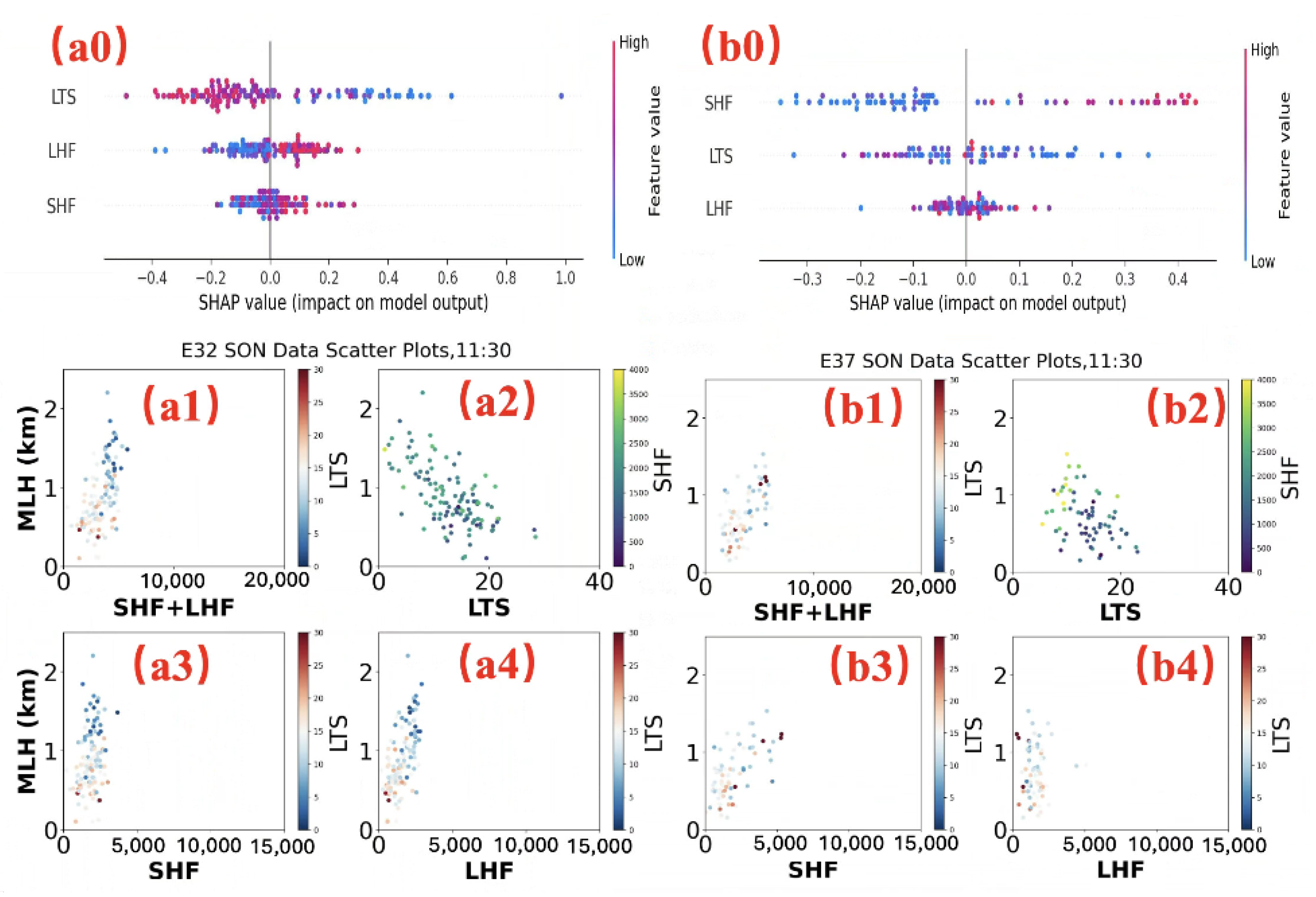
40], a widely-used tool for interpreting machine learning model predictions. SHAP, rooted in Shapley values from game theory, explains model outputs by attributing contributions to each feature. These SHAP values quantify the impact of each feature on the prediction, allowing researchers to elucidate the model’s decision-making process, identify key contributing factors, and improve model performance. Specifically, positive SHAP values reflect a feature’s positive contribution to the MLH, a value of 0 indicates no influence and negative SHAP values signify a negative contribution, where an increase in the feature value reduces MLH. The results derived from our model are illustrated in
Figure 5, where (a0) and (b0) depict the SHAP value beeswarm [
39] plots for the E32 and E37 sites, respectively. And the a1–a4, and b1–b4 are the scatter plots of SHF, LHF, and LTS with MLH for the E32 and E37 sites, respectively.
Figure 5(a0) shows a predominantly negative correlation between LTS and SHAP values. Similarly,
Figure 5(a2) also indicates a negative correlation, though it is less pronounced than in
Figure 5(a0). Additionally,
Figure 5(a0) reveals a positive correlation between LHF and SHAP values, a trend further supported by the scatter plot in
Figure 5(a4). In contrast,
Figure 5(b0) demonstrates that the correlation between LHF and SHAP values at the E37 site is weaker than at the E32 site, a pattern also reflected in
Figure 5(b4). Meanwhile,
Figure 5(b0) highlights a positive correlation between SHF and SHAP values, which is confirmed by the scatter plot in
Figure 5(b3). However, the relationship between SHF and SHAP values in
Figure 5(a0) is less evident, as shown in the scatter plot in
Figure 5(a3). Notably,
Figure 5(a1,5b1) demonstrate that the combined SHF and LHF exhibit a positive correlation with MLH. Specifically, at the ARM SGP sites, such as E37 and E32, which are approximately 57 km apart, these findings highlight the influence of local parameters (SHF and LHF) over broader meteorological conditions, as LTS remains relatively consistent across sites while SHF and LHF vary significantly. While the total SHF + LHF remains similar, the distribution between SHF and LHF is largely influenced by local factors.
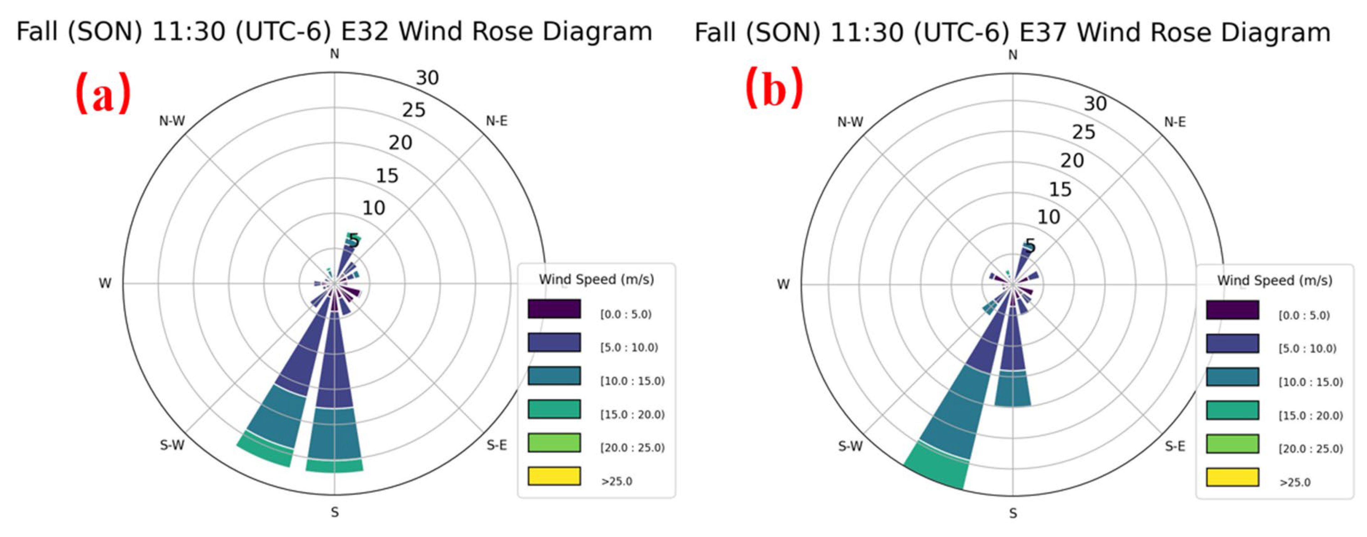
By analyzing the SHAP values of the model, we can clearly understand how the differences in relative influencing factors between different sites are determined. However, further investigation is needed to identify the underlying causes of these differences. In addition to local factors, wind direction appears to correlate with relative impact factors. To examine this relationship, wind rose diagrams were generated for each site across different seasons, using data over identical day counts as in
Figure 5, with results presented in
Figure 6. By comparing
Figure 4 and
Figure 6, we aim to clarify certain differences in relative impact factors. By comparing
Figure 4 and
Figure 6, we seek to elucidate differences in relative influence factors across sites and seasons. As depicted in
Figure 4, during the SON season, LHF is more influential at site E32 (~0.50), whereas SHF predominates at site E37 (>0.60). Analysis of wind direction in
Figure 7 indicates that, at E32 during SON, winds primarily originate from the south (180 ± 15°) and southwest (210 ± 15°), each with a probability of approximately 27%. At E37, southwest winds (210 ± 15°) occur with a higher probability (>30%), significantly exceeding the 15% probability of south winds (180 ± 15°). This difference suggests that south winds, which are typically more humid, enhance latent heat flux (LHF), whereas south-southwest winds, often drier, contribute less moisture. Consequently, LHF remains relatively stable at approximately 0.35 during JJA, likely reflecting the influence of prevailing humid south winds in the summer season.
The discussion above demonstrates the effectiveness of machine learning in analyzing the relative impacts of factors such as SHF, LHF, and LTS on boundary layer processes. However, the analysis focused on wind direction as an example to explore seasonal variations in relative impact factors across different locations. ABL drivers are inherently complex and dynamic, and thus, focusing solely on instantaneous values of SHF, LHF, and LTS is insufficient. Future research should incorporate additional boundary layer parameters and investigate how these factors interact dynamically to influence boundary layer development over time.
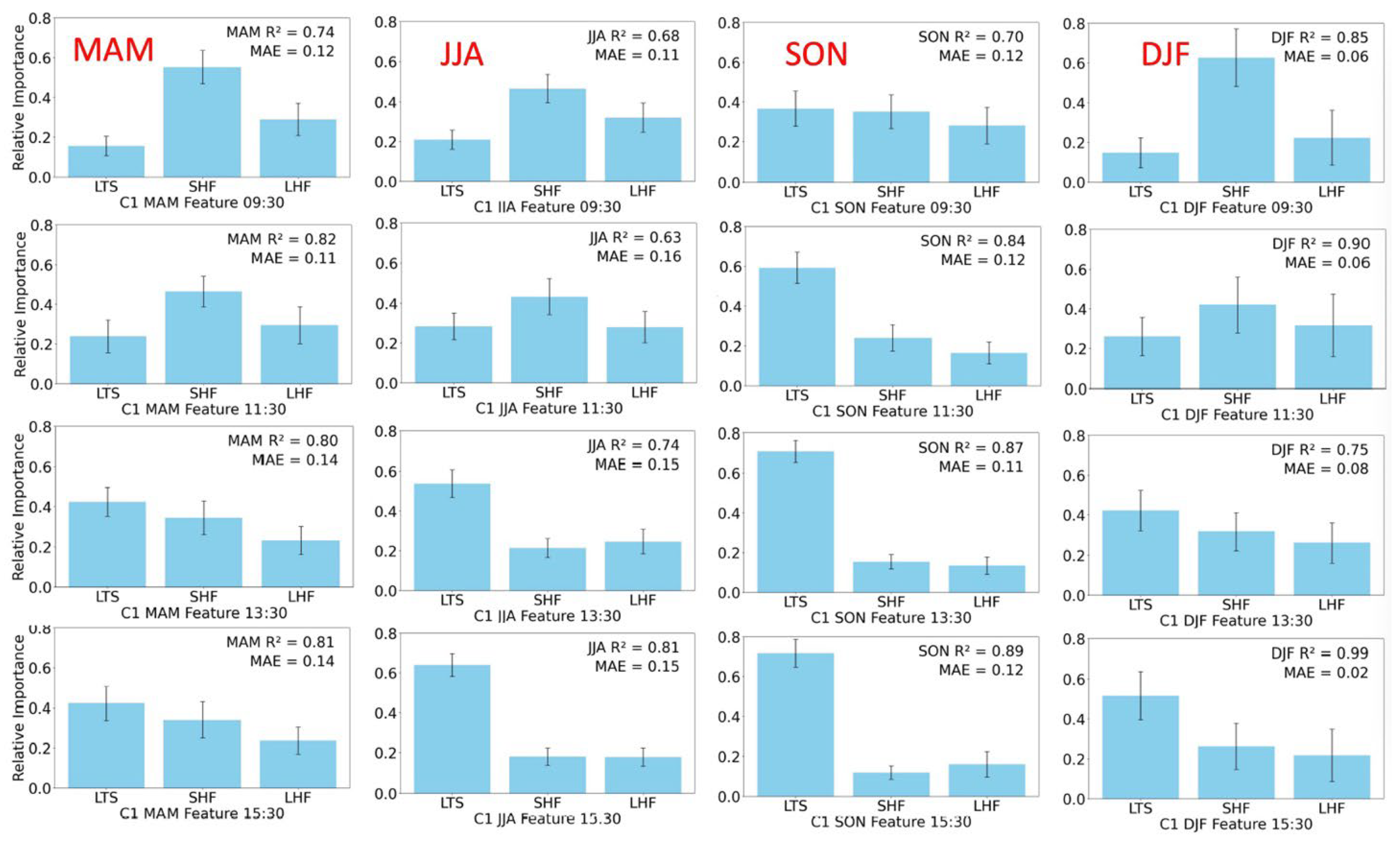
To further investigate the variations in relative importance across different seasons and time points, we analyze the changes at specific hours throughout the day. As shown in
Figure 7, we evaluate four distinct time points from 9:30 AM to 3:30 PM, sampled at two-hour intervals across all four seasons. A notable trend is observed in the relative importance of LTS, which gradually increases from the morning to the afternoon across all seasons. Taking JJA as an example, the relative importance of LTS starts at approximately 0.2 at 9:30, increases to 0.28 at 11:30, reaches 0.4 at 13:30, and further rises to 0.6 at 15:30. This suggests that as the ABL develops, the role of LTS becomes increasingly significant. Initially, the ABL is less influenced by LTS, but as it grows towards the ABL top, a higher LTS necessitates a stronger flux-driven mechanism. This observation aligns well with ABL evolution theories, as discussed in the published literature on ABL [
7,
13,
18].
Moreover, the SON season exhibits distinct characteristics. At 9:30 AM, the relative importance of LTS is close to 0.4, significantly higher than the other three seasons, where it remains below 0.2. This indicates that during autumn, the boundary layer reaches its top more rapidly. Conversely, in winter (DJF), the LTS at 9:30 AM is below 0.2, and despite a steady increase throughout the day, it only reaches approximately 0.4 at 3:30 PM. This suggests that during spring (MAM), the MLH encounters greater resistance in reaching the previous day’s boundary layer top. Additionally, comparing JJA and SON, the LTS during summer starts at 0.2 at 09:30 AM and increases to 0.6 at 3:30 PM, consistently lower than its autumn counterpart at corresponding time points. While summer exhibits stronger heat flux and a lower average LTS, the ascent rate of the ABL remains slower than in autumn. The reason for this phenomenon is that the relative importance of LTS gradually increases from morning to noon, indicating that LTS becomes more critical as the ABL approaches its maximum height. This occurs because further growth beyond the boundary layer top requires significantly more energy, and LTS represents the thermal energy needed to reach this threshold [
9]. Consequently, the LTS at 9:30 in autumn (SON) exhibits greater relative importance compared to other seasons. This reflects a more rapid development of the MLH in autumn, suggesting that residual layers from precipitation may facilitate easier attainment of the ABL height from the previous day. Thus,
Figure 7 provides valuable insights into the seasonal evolution of the ABL.
An interesting observation in DJF is that the MAE values remain below 0.1, with some as low as 0.02, while the R² values range from 0.75 to 0.99. Despite these seemingly favorable metrics, the error bars for relative importance are larger than those of other seasons, indicating significant fluctuations in model predictions. This instability is primarily attributed to data limitations: despite employing K-fold cross-validation, the effective data sample for DJF remains small, with only 60 days of observations, whereas JJA contains 156 days. Consequently, the model in DJF leads to higher variance in importance scores.
6. Conclusions
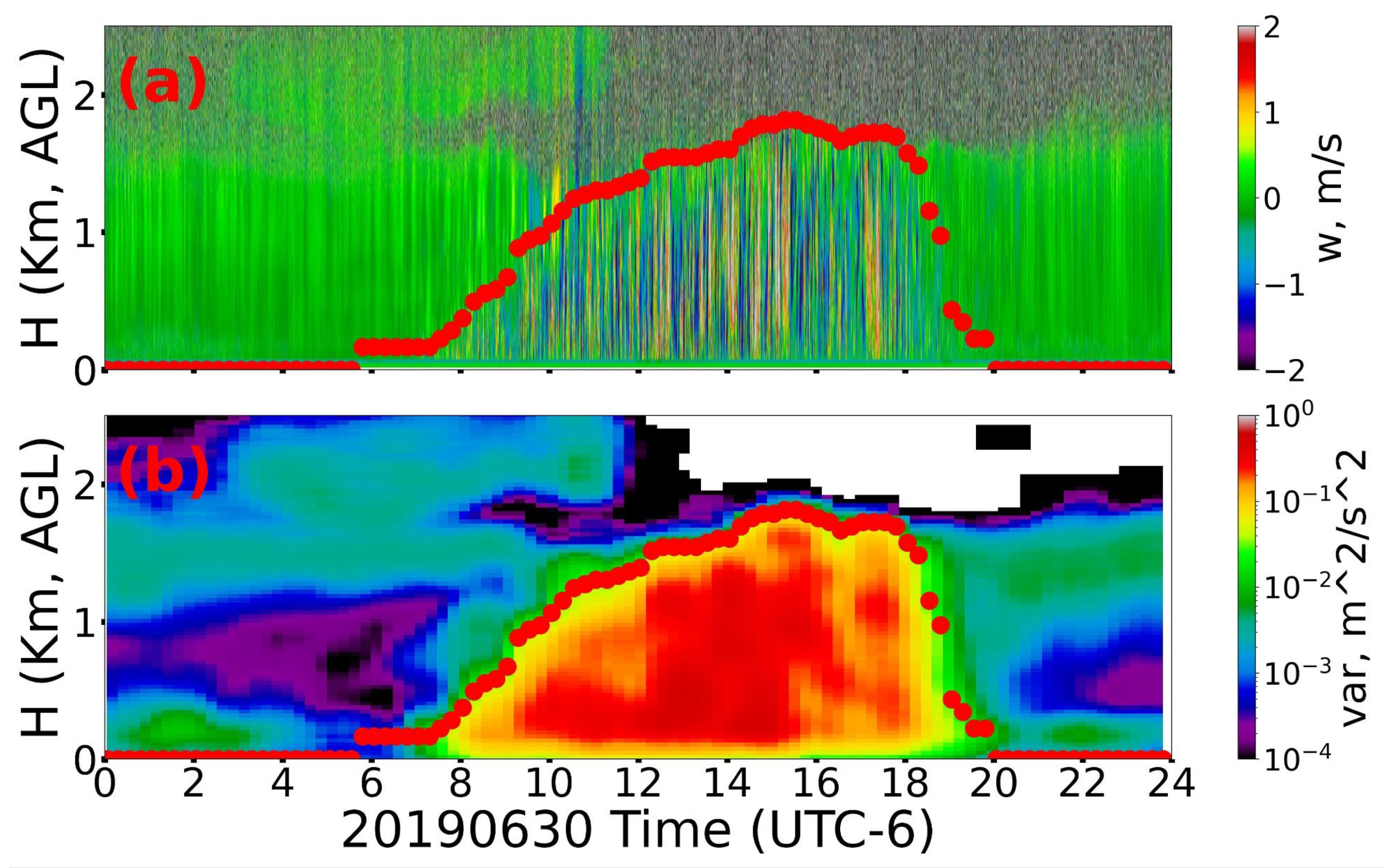
This study integrates XGBoost and cross-validation to analyze the relative importance of ABL driving factors in atmospheric research. While XGBoost has been applied in this field, it often relies on default parameters. Additionally, due to the challenges of acquiring long-term, multi-parameter meteorological data, it has not been widely used to study seasonal variations in driving factor importance. To address this, we focus on key thermodynamic drivers of the boundary layer, selecting LTS, SHF, and LHF as primary influencing factors. We use Doppler lidar vertical wind field data to derive MLH as an indicator of CBL evolution. This study examines the effects of different parameter settings and optimizes hyperparameters based on the actual research dataset. Without cross-validation, the correlation coefficient R2 from different XGBoost models fluctuates significantly, ranging from 0.47 to 0.83, with relative influence factors varying by more than 0.10. When cross-validation is applied with default parameters, the R2 value remains stable across different splits, but factor importance still varies by over 0.10, with only around 0.60. By using optimized parameters, both R and relative influence factors remain stable within a 0.03 range, achieving an R2 value of 0.81. Based on these results, we analyzed seasonal variations in relative influence factors at the C1 site, providing insights for applying similar methods in atmospheric studies.
Subsequently, the results of different seasons demonstrate significant seasonal variations in the relative influence of key atmospheric factors, deviating from the annual trends. While LTS dominates in summer at the C1 site (0.6), SHF plays a more dominant role in other seasons (MAM: 0.5, JJA: 0.42, DJF: 0.4). The increased number of data points in JJA and SON causes LTS to appear as the dominant factor in the annual analysis (~0.5,
Table 3). However, seasonal differences are evident, with JJA exhibiting a lower R
2 (0.63) despite having more data points, indicating that ABL development in summer is influenced by additional meteorological factors or more complex controlling mechanisms. Notably, during JJA, the differences in the relative importance of the three factors across all sites are low. This suggests that boundary layer development in summer is not dominated by a single factor, indicating a more complex process likely influenced by seasonal conditions such as enhanced convective activity, elevated temperatures, and increased humidity. These factors collectively contribute to a more balanced distribution of parameter impacts. However, these interpretations remain speculative and require further validation. MLH variations further confirm that its peak occurs in SON, where LTS plays a stronger role, particularly at C1 and E37. E39 shows a more balanced contribution from LTS, SHF, and LHF, but its higher variance, especially in SON, suggests that dataset size significantly impacts result reliability. Additionally, MAE values and dataset quality must be considered, as DJF consistently shows the lowest MAE (<0.1) due to inherently lower MLH, while JJA exhibits the highest MAE (~0.16 at E32), if an annual model were used, MAE would exceed 0.15, reflecting greater model uncertainty. These findings highlight the necessity of further research into localized atmospheric processes affecting ABL dynamics, as ABL evolution is highly sensitive to seasonal and regional variations in stability, surface fluxes, and local meteorological conditions.
We further analyzed the differences between E32 and E37 during autumn (SON) using SHAP and explored potential reasons for the discrepancies between the two sites through wind direction analysis with WIND ROSE figures. These findings highlight the intuitive and significant role that SHAP can play in considering the seasonal variations of influencing factors when analyzing different locations. Later, XGBoost expanded upon this by attempting to quantify the relative influence of different parameters on ABL development [
13]. In this study, we integrate XGBoost with cross-validation to explain the relative influencing factors of various parameters on ABL development across different seasons.
Our analysis reveals significant seasonal variations in the relative importance of LTS in ABL evolution. Across all seasons, the LTS importance increases from morning to afternoon, with JJA rising from 0.2 at 09:30 AM to 0.6 at 3:30 PM, indicating its growing influence as the boundary layer develops. SON exhibits the highest LTS importance at 09:30 AM (~0.4), suggesting a faster ABL growth compared to other seasons. In contrast, DJF shows the lowest LTS values in the morning (<0.2), with a slower increase throughout the day, implying greater difficulty in reaching the previous day’s ABL top. Additionally, DJF exhibits potential overfitting issues, with MAE values consistently below 0.1 (as low as 0.02) and R² ranging from 0.75 to 0.99, likely due to a limited dataset (60 days vs. 156 days in JJA). These findings highlight the role of LTS in ABL dynamics and emphasize the need for more extensive wintertime data to improve model robustness.
To the authors’ knowledge, this study represents the first application of machine learning to investigate the relative importance of various meteorological parameters on ABL development across different locations and seasons. This study not only examines the relative importance of influencing factors at the C1 site throughout the year and across seasons but also compares their variations across multiple ARM SGP sites. Additionally, an attempt is made to use wind direction to distinguish differences in relative impact factors between sites. However, a more detailed investigation is needed to understand the specific differences in ABL evolution and the seasonal variations in influencing factors across the four sites [
13]. Since this study investigates changes in the relative importance of parameters, it can provide valuable insights for refining machine learning frameworks in the future and contribute to developing models that approach or exceed the performance of traditional PBL schemes.
Despite certain limitations, such as focusing only on thermodynamic influences while neglecting dynamical factors, and without considering the full ABL evolution process, this study serves as an exploratory application of machine learning in atmospheric research. It highlights the importance of incorporating domain-specific scientific principles into machine learning tools like XGBoost to optimize parameters and ensure accurate results. This study initially focuses on thermodynamic parameters, acknowledging that the omission of dynamical factors (e.g., wind shear, advection) limits the theoretical foundation of the model. These dynamical factors play a critical role, particularly when the MLH nears the boundary layer top, where their absence may amplify discrepancies between predictions and observations. Nevertheless, the current approach can be extended to incorporate additional boundary layer drivers, such as wind speed, wind direction, terrain, vegetation, water vapor, and cloud properties [
41,
42,
43,
44,
45,
46]. Future research should integrate these dynamical factors to enhance the model’s theoretical robustness and predictive accuracy, as suggested by recent studies on gravity waves, wind shear, and stratospheric disturbances. Additionally, integrating machine learning with numerical models can provide a more comprehensive understanding of boundary layer dynamics [
47].


