
A Deep Learning Method for Land Use Classification Based on Feature Augmentation

 ,
,
Abstract
1. Introduction
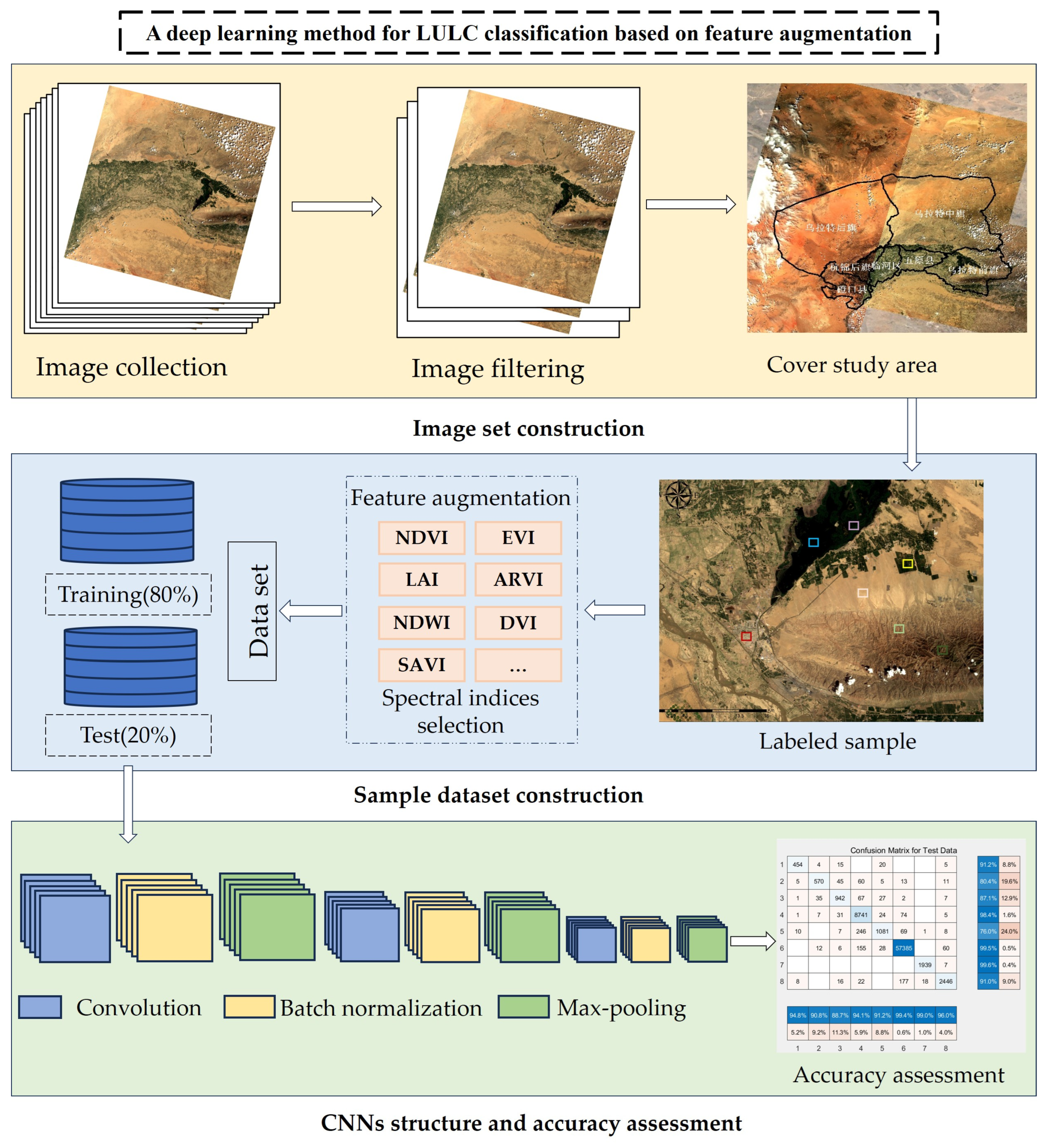
2. Methods
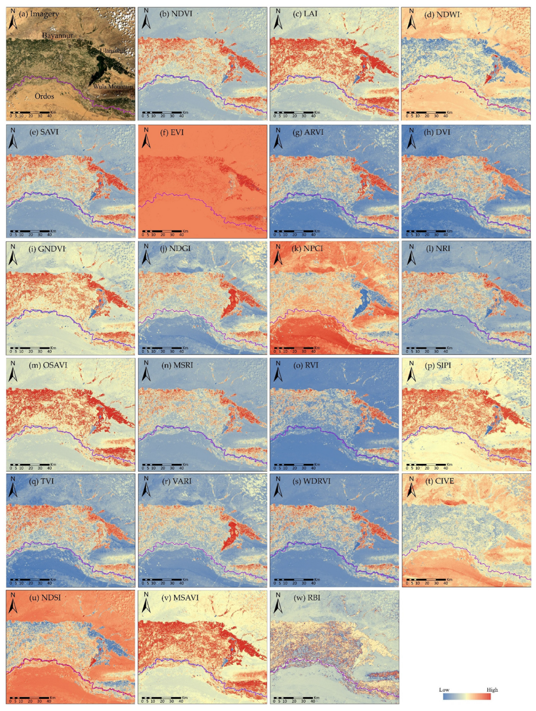
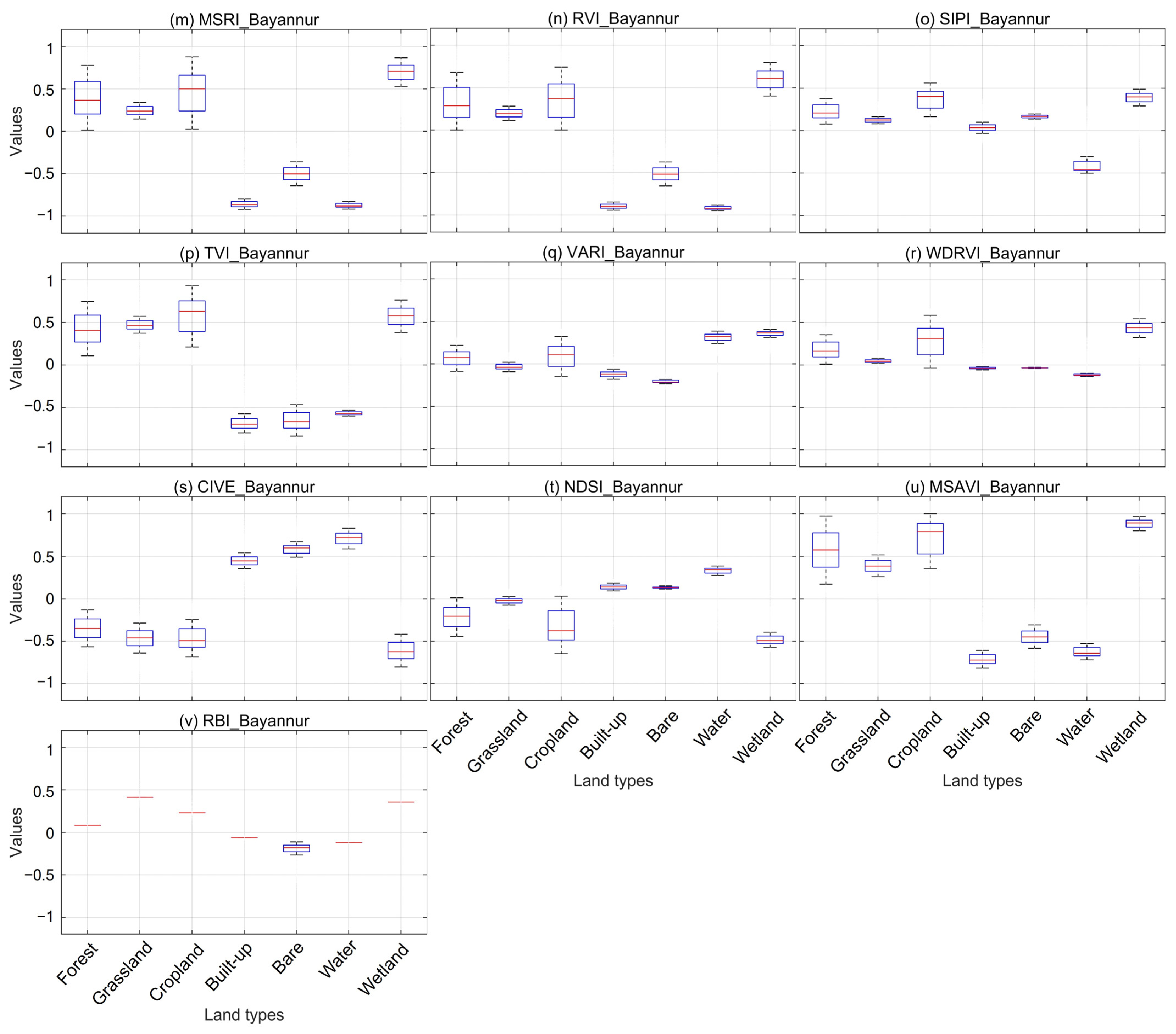
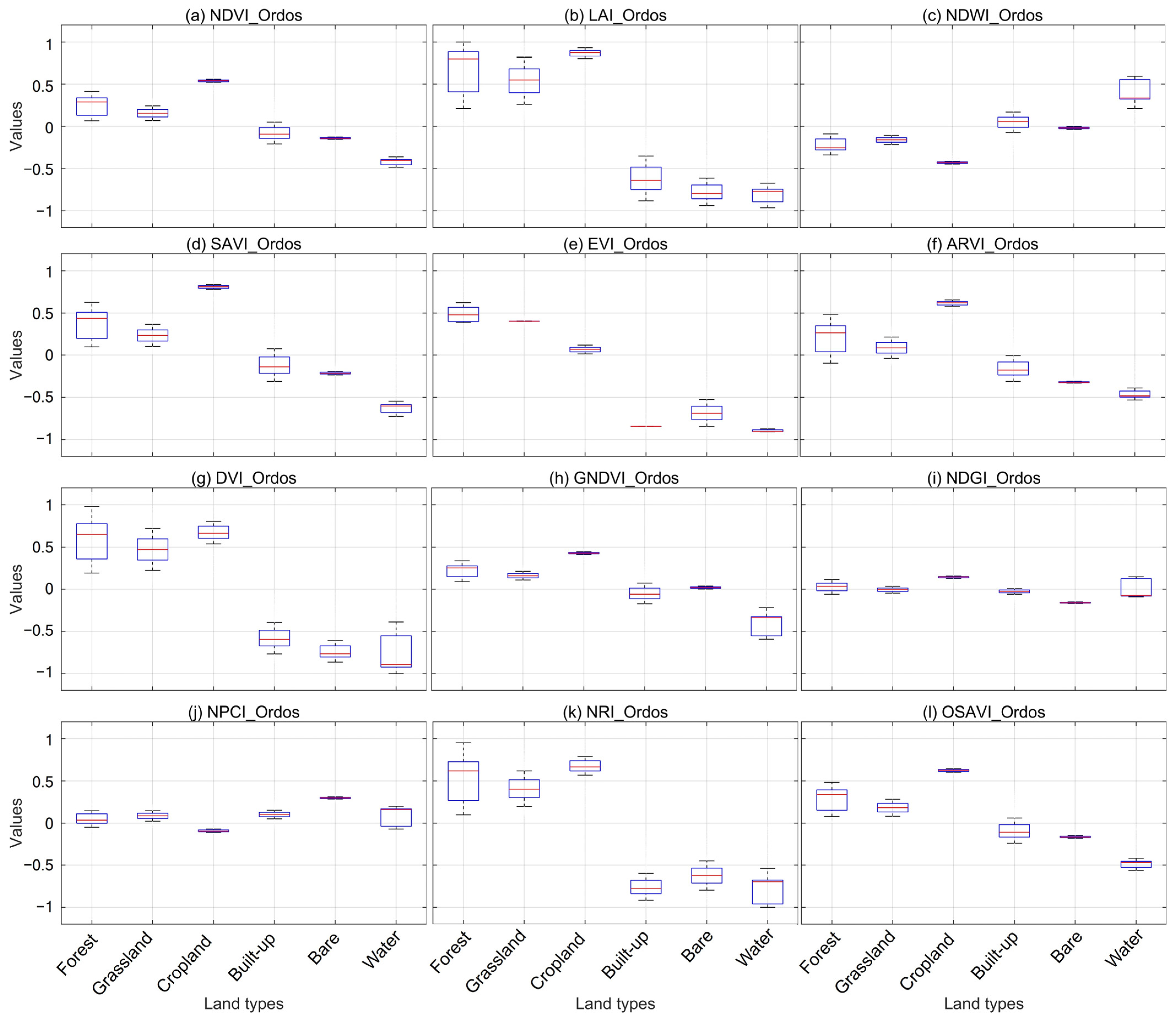
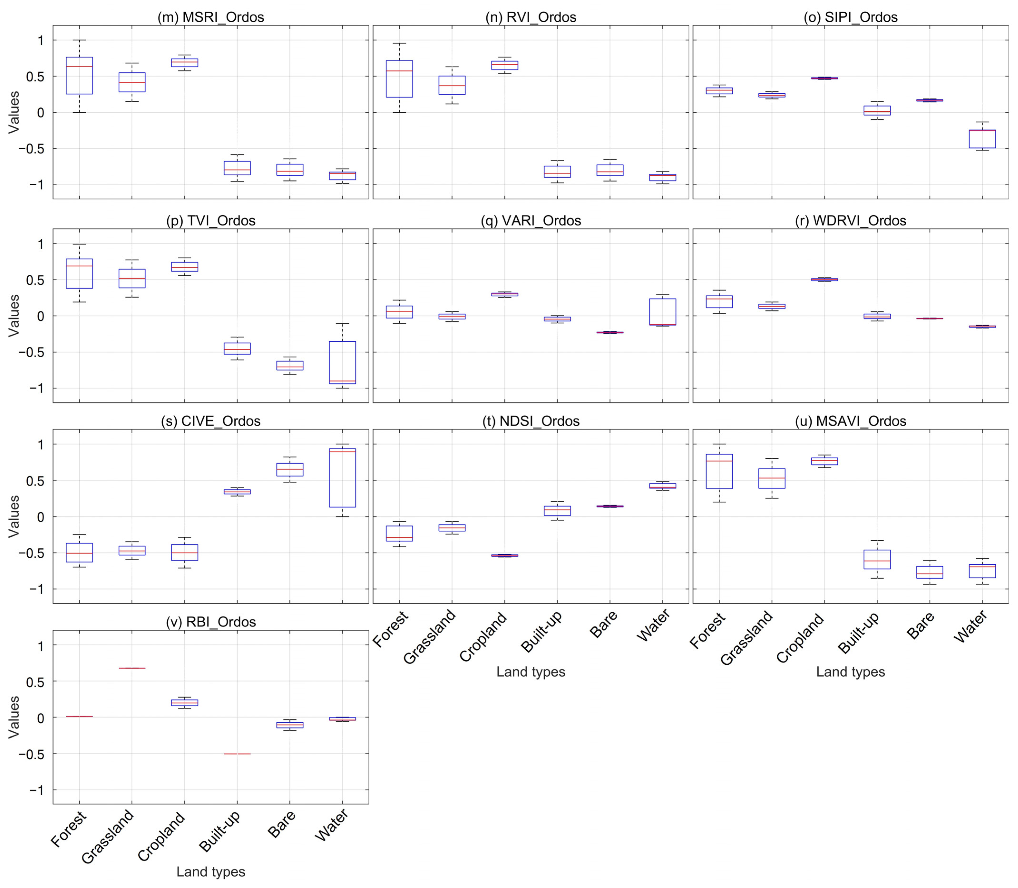
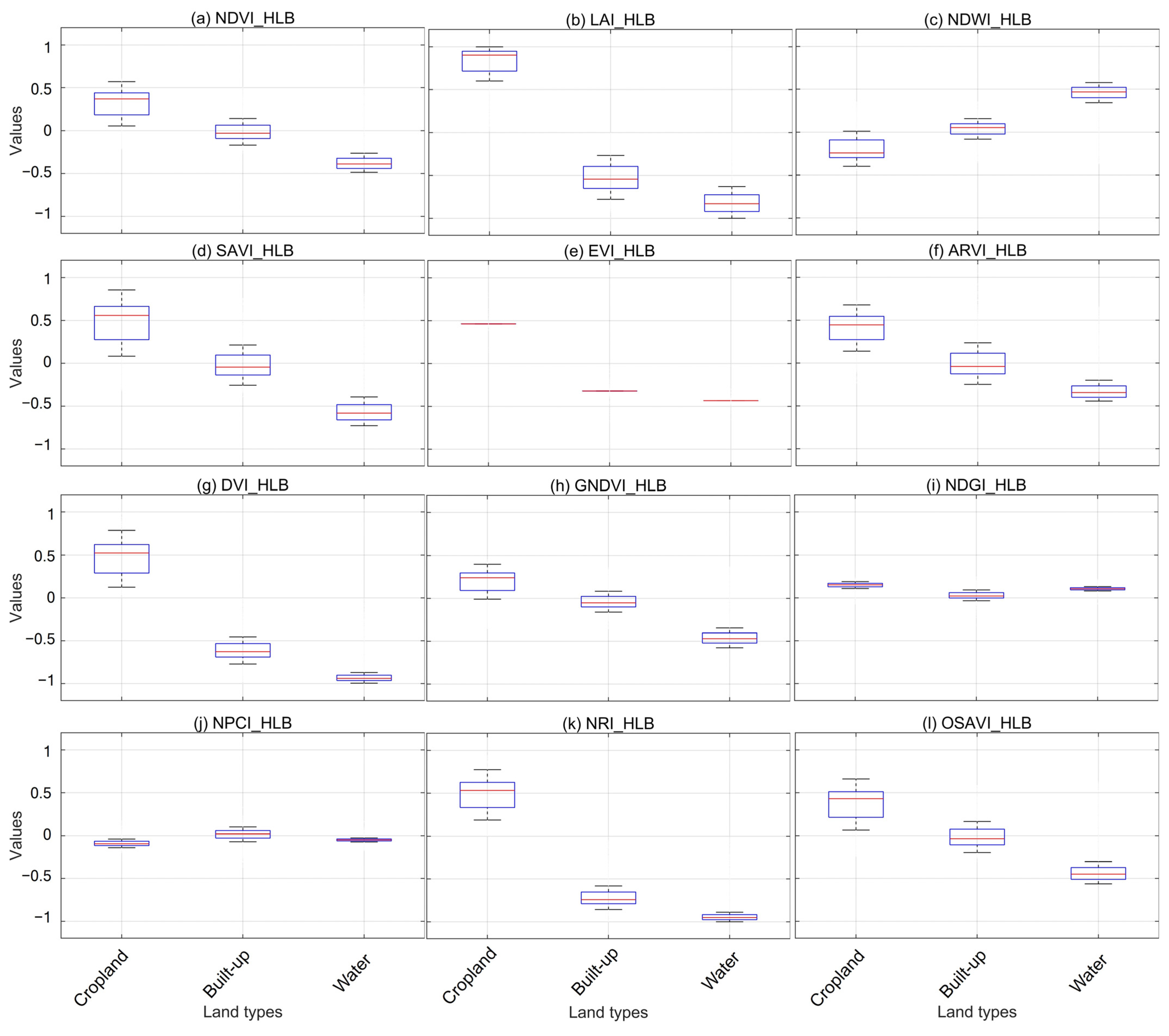
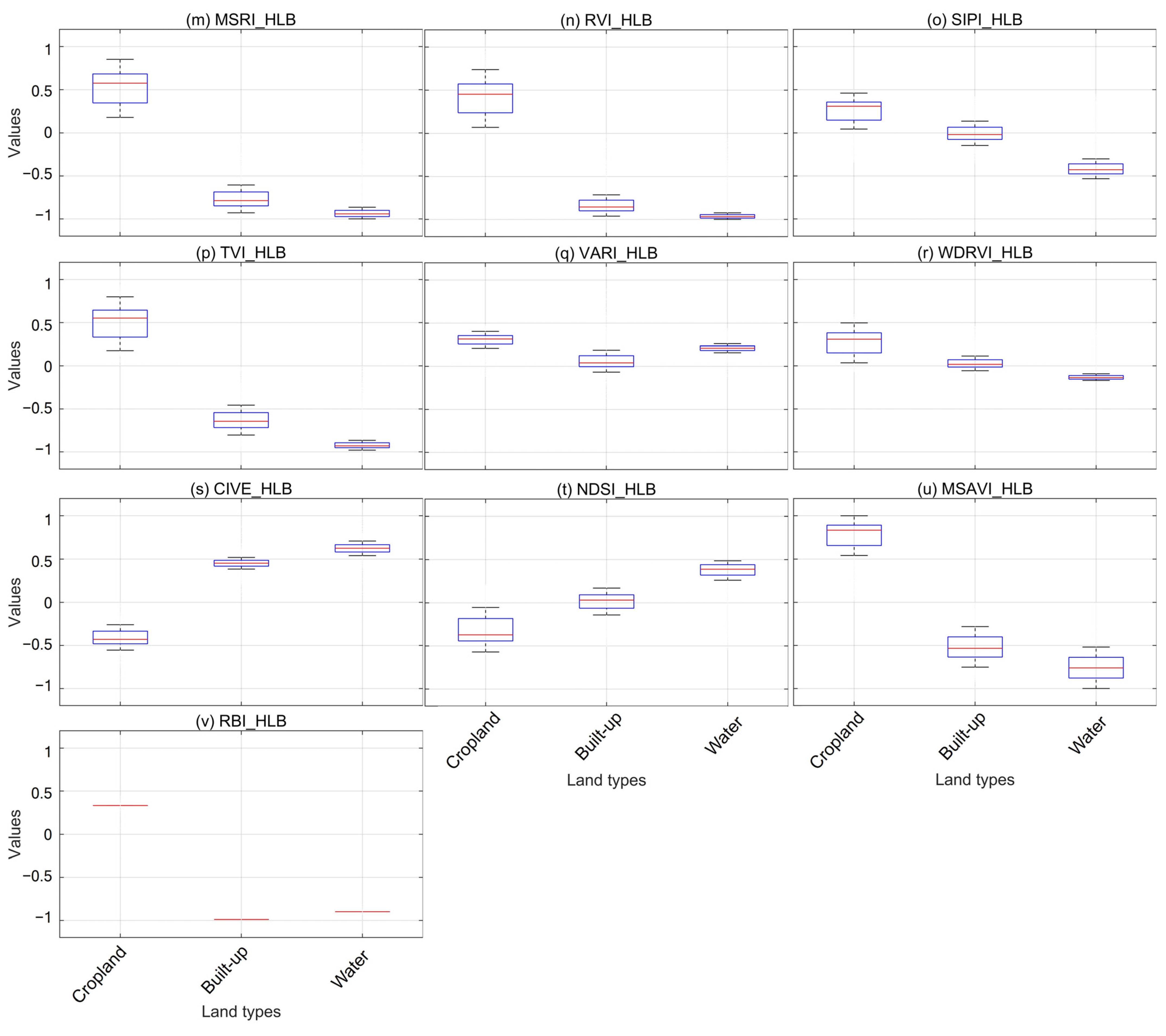
2.1. Spectral Indices Selection
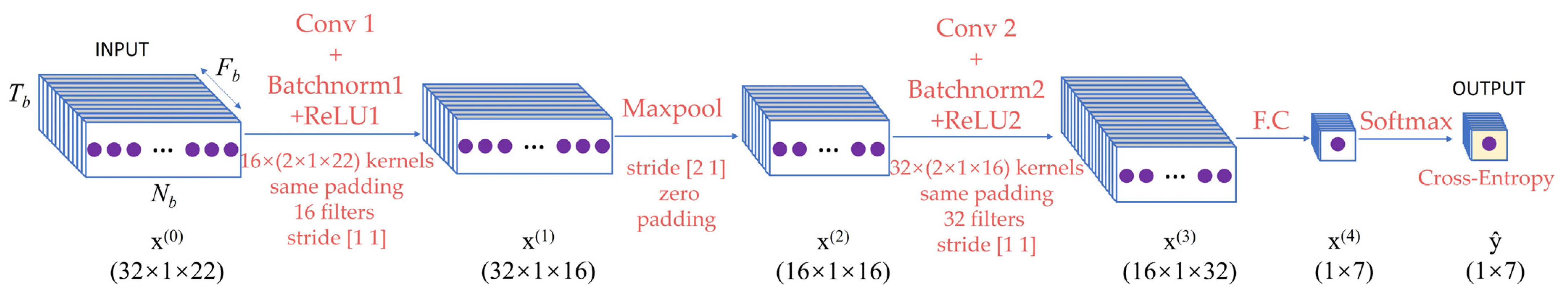
2.2. CNN Structure
2.3. Image Set Construction
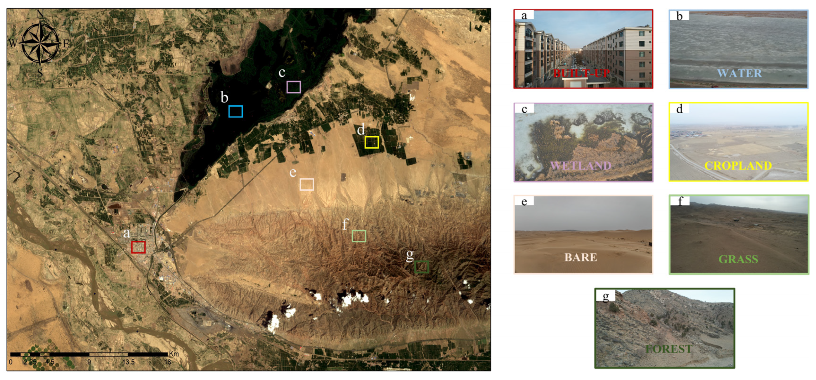
2.4. Sample Labeling
2.5. Accuracy Assessment
- (1)
- Model accuracy assessment
- (2)
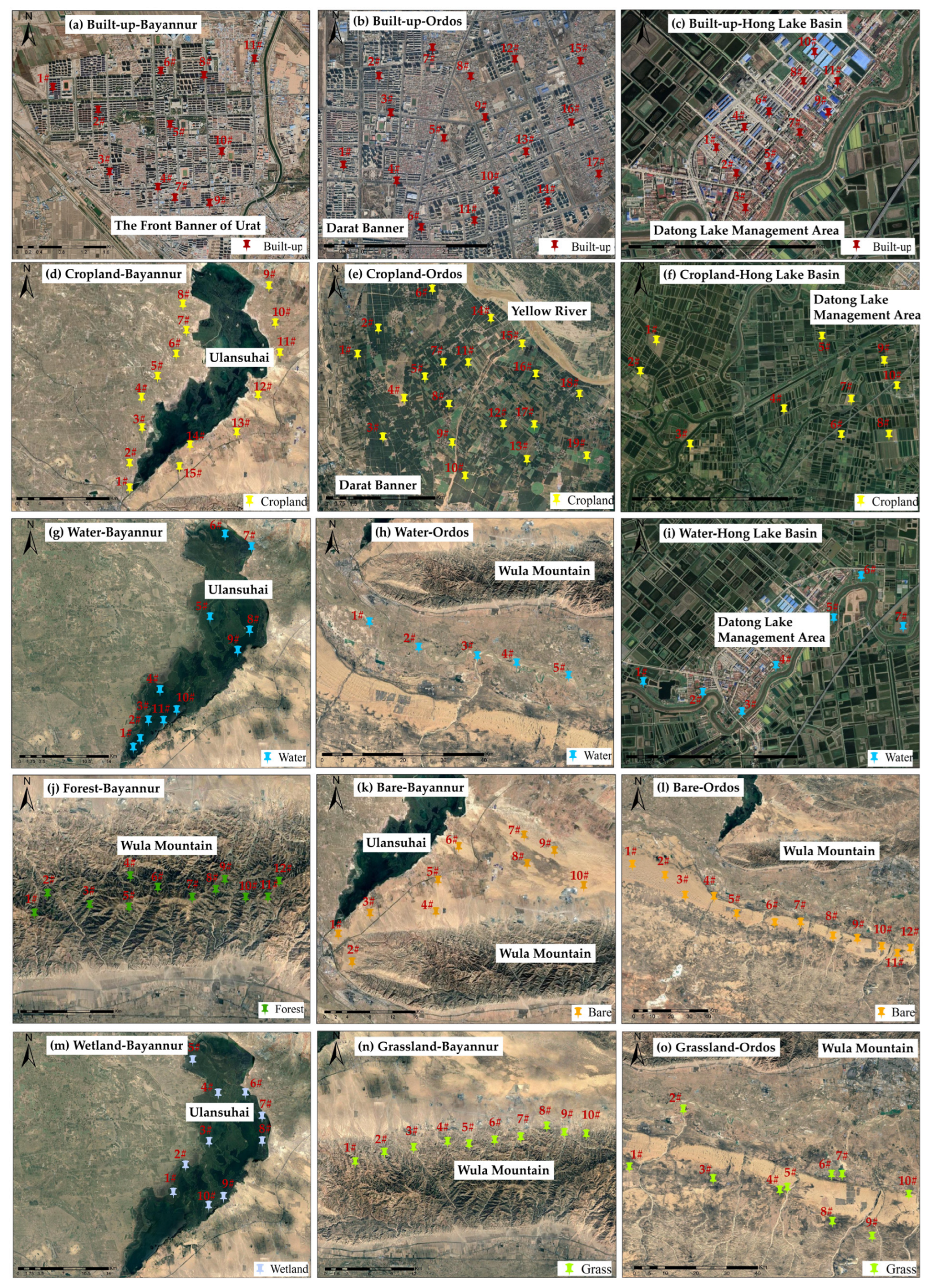
- Field validation
2.6. Method Feasibility Analysis
3. Results
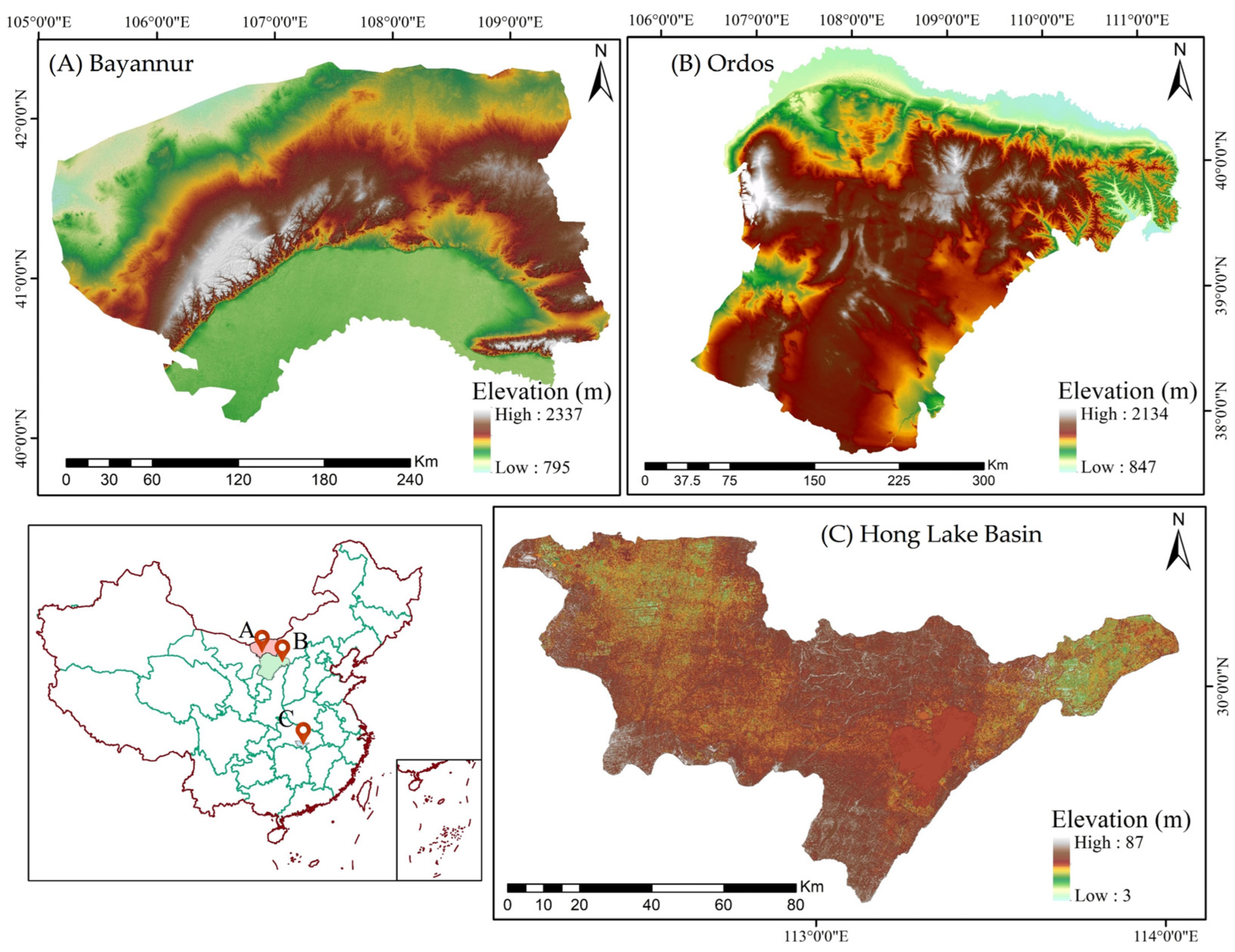
3.1. Study Area and Data Source
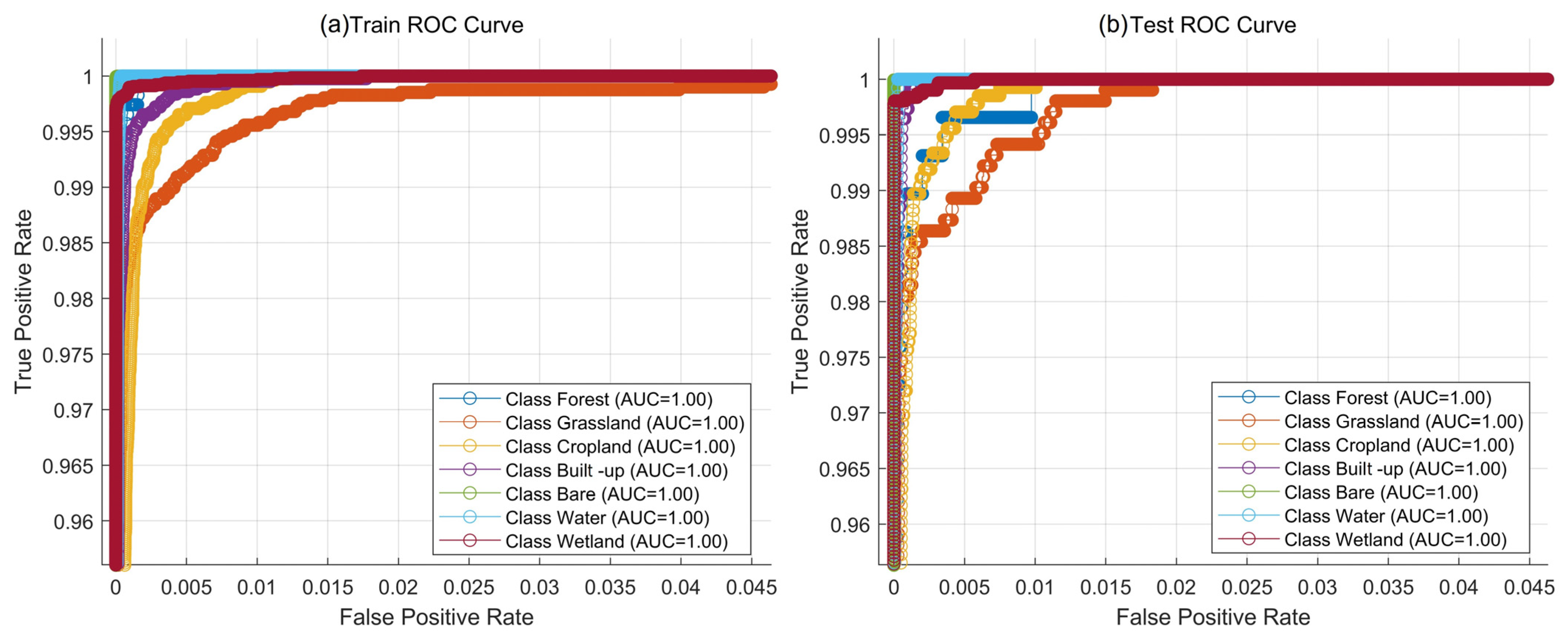
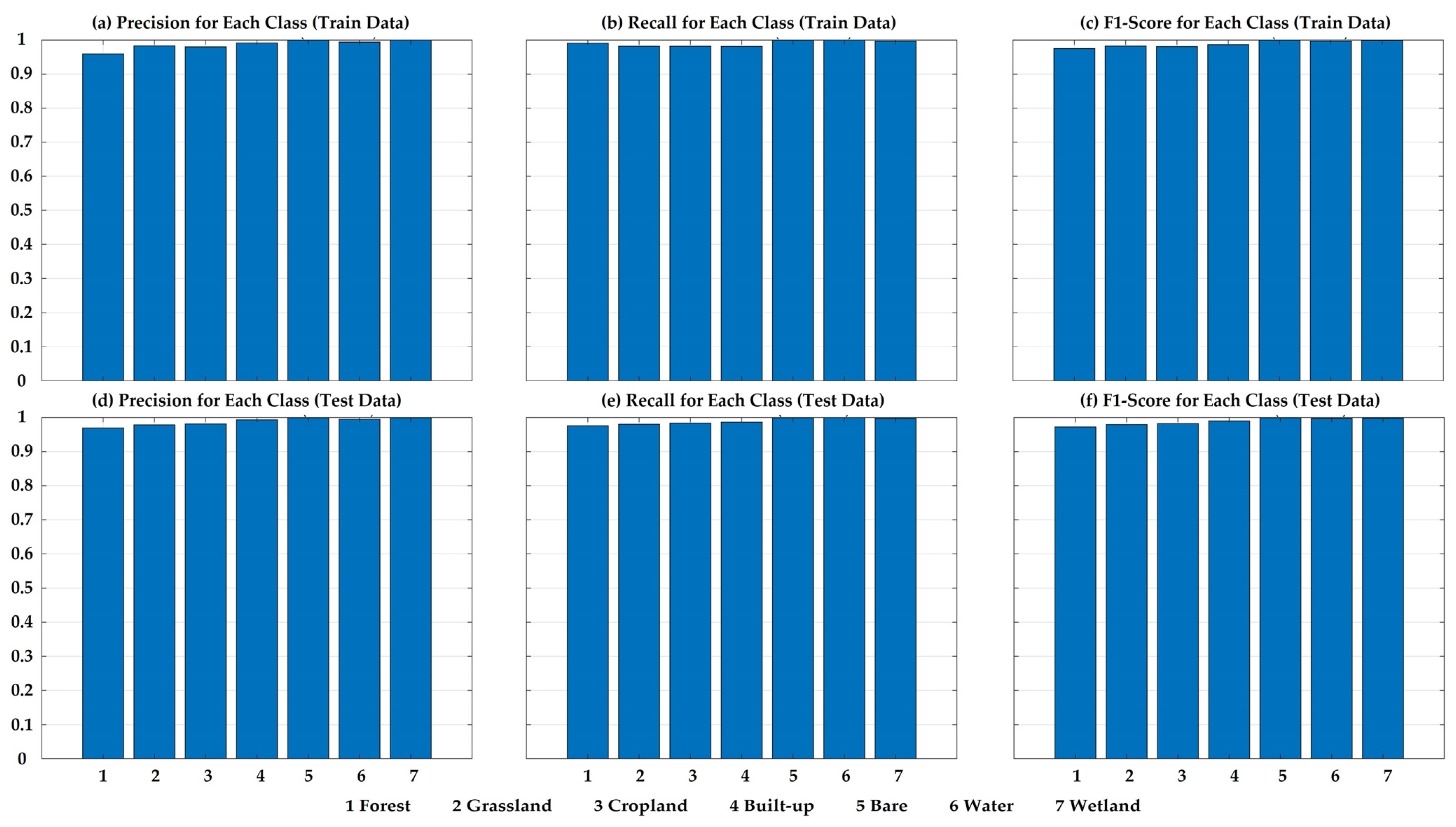
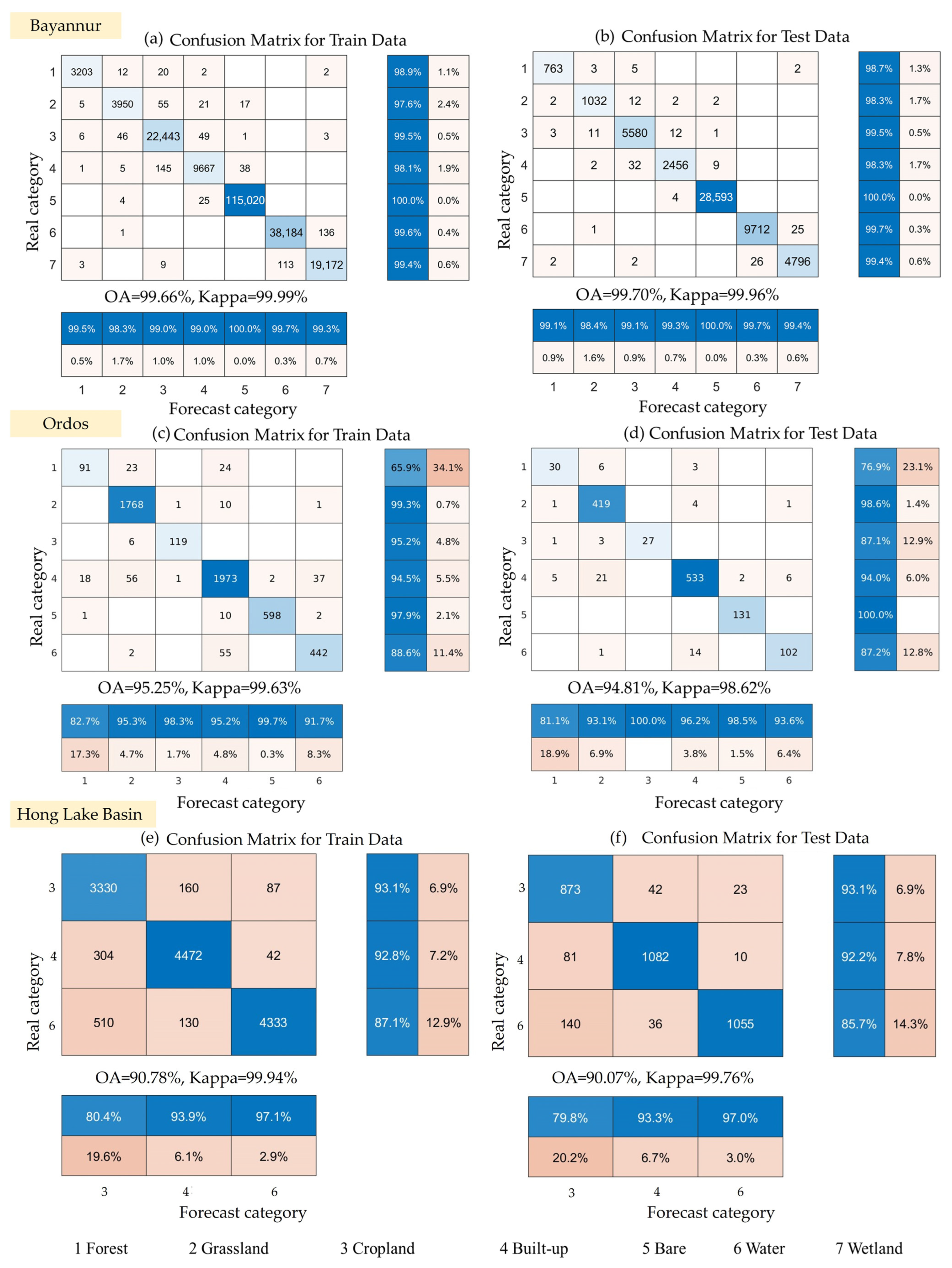
3.2. Accuracy Assessment Results
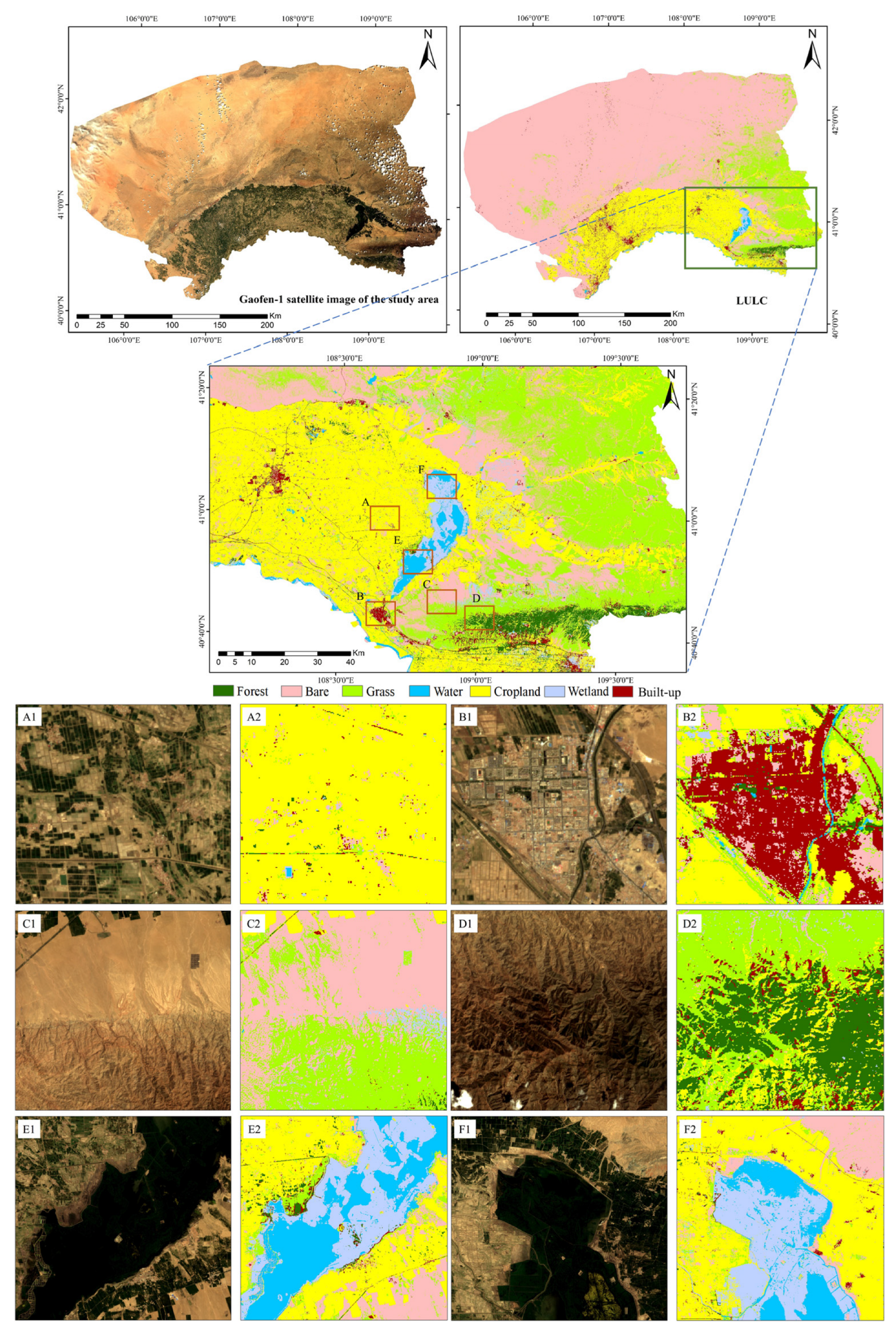
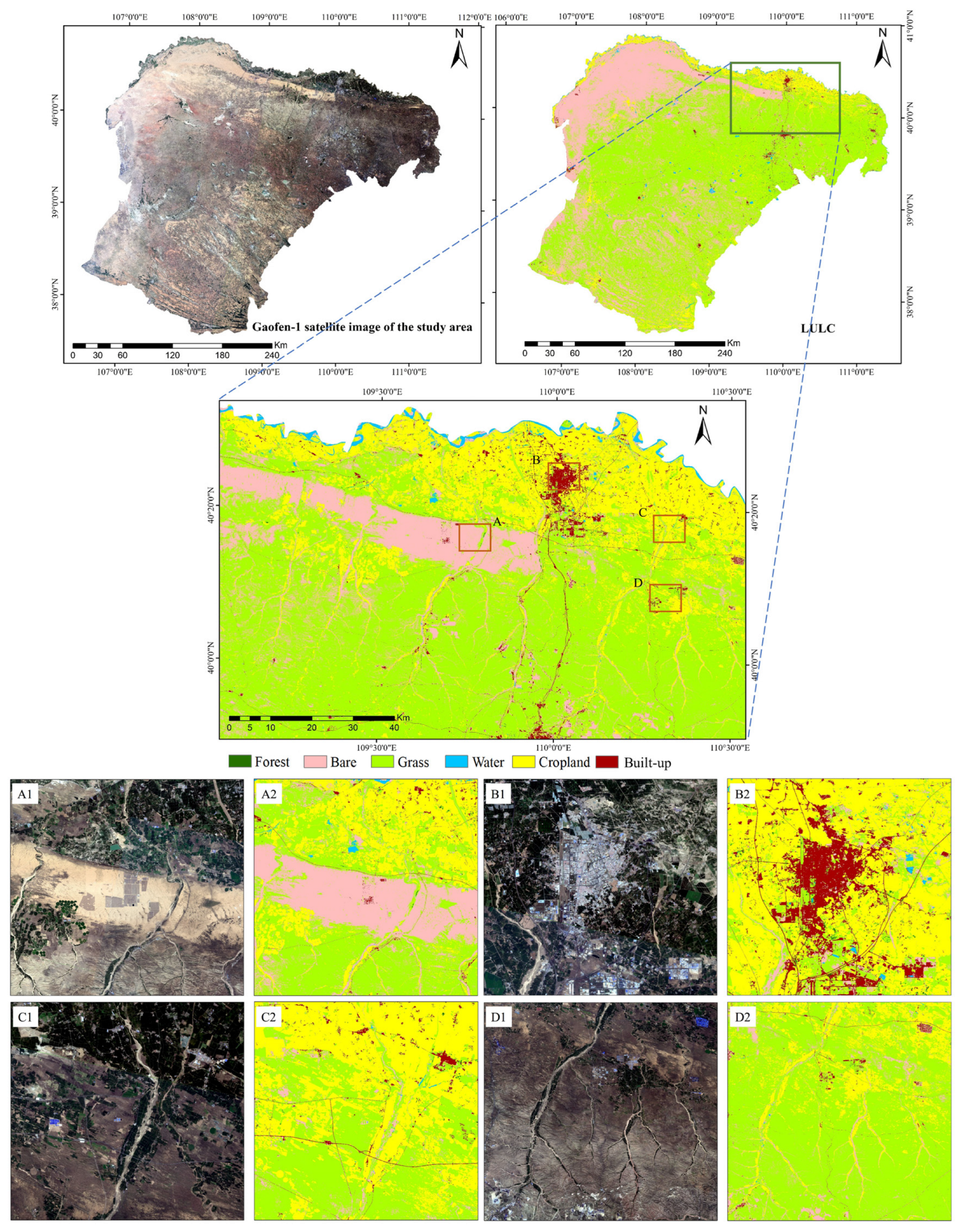
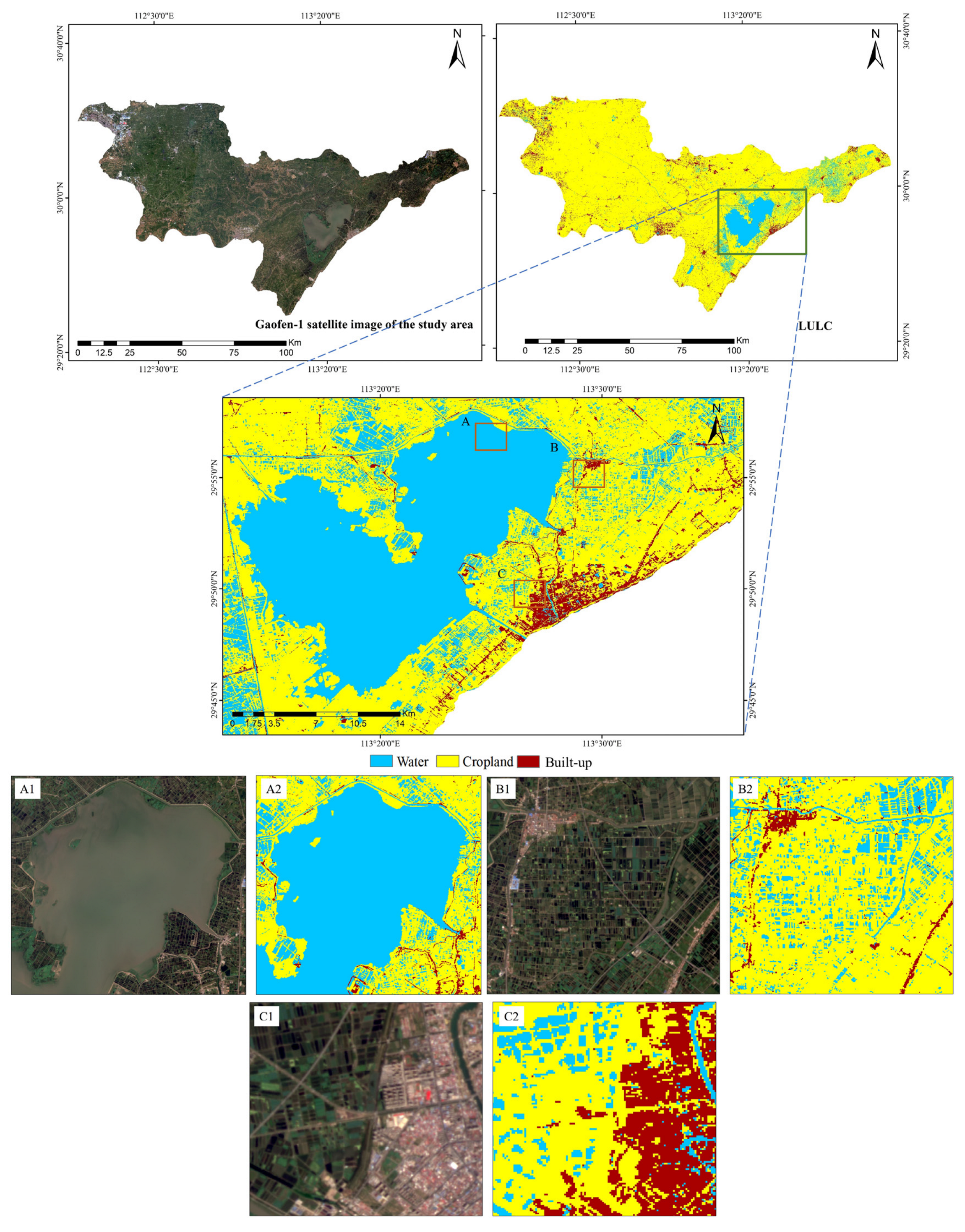
3.3. Land Use Classification
- (1)
- Bayannur
- (2)
- Ordos
- (3)
- HLB
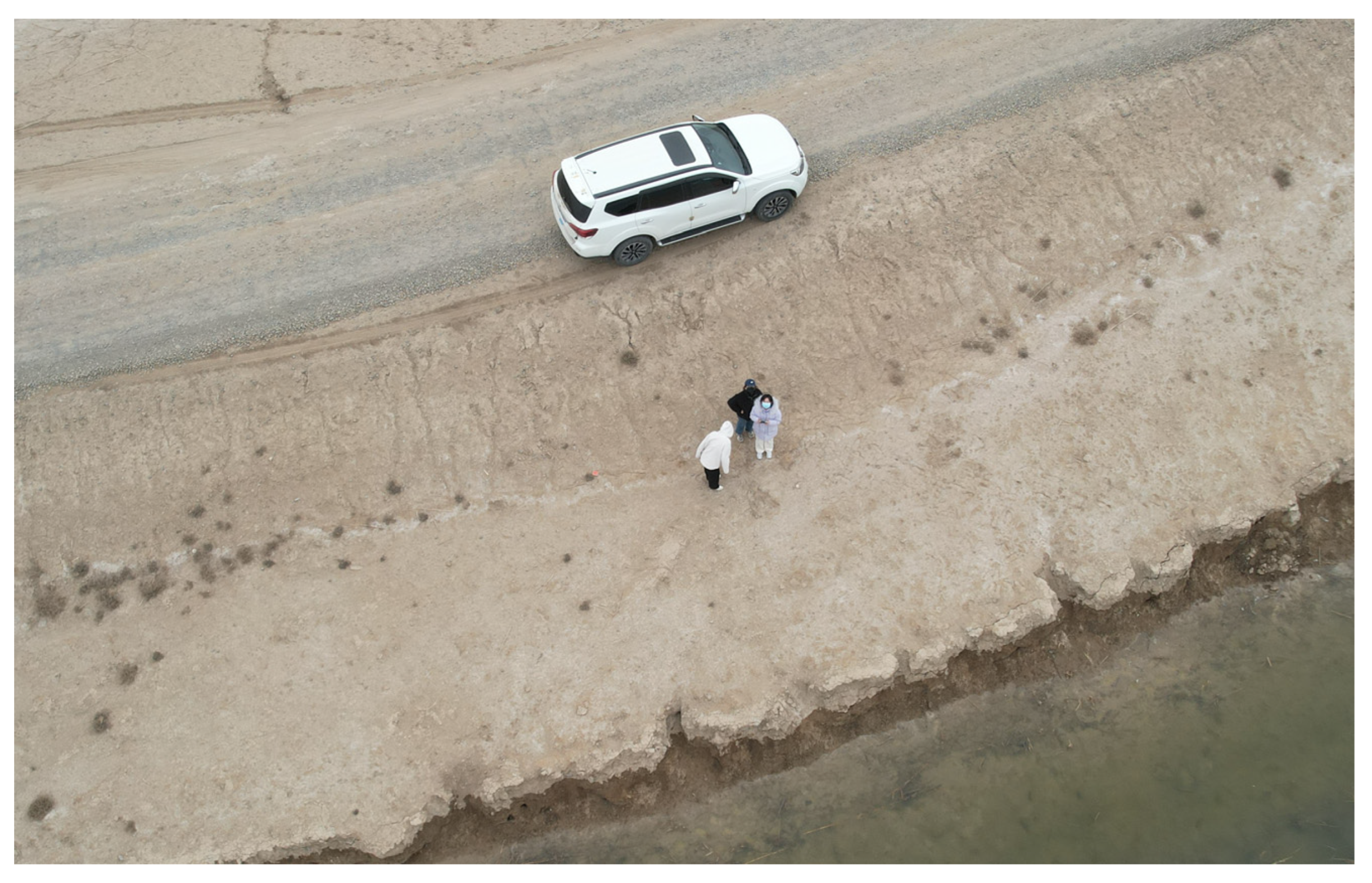
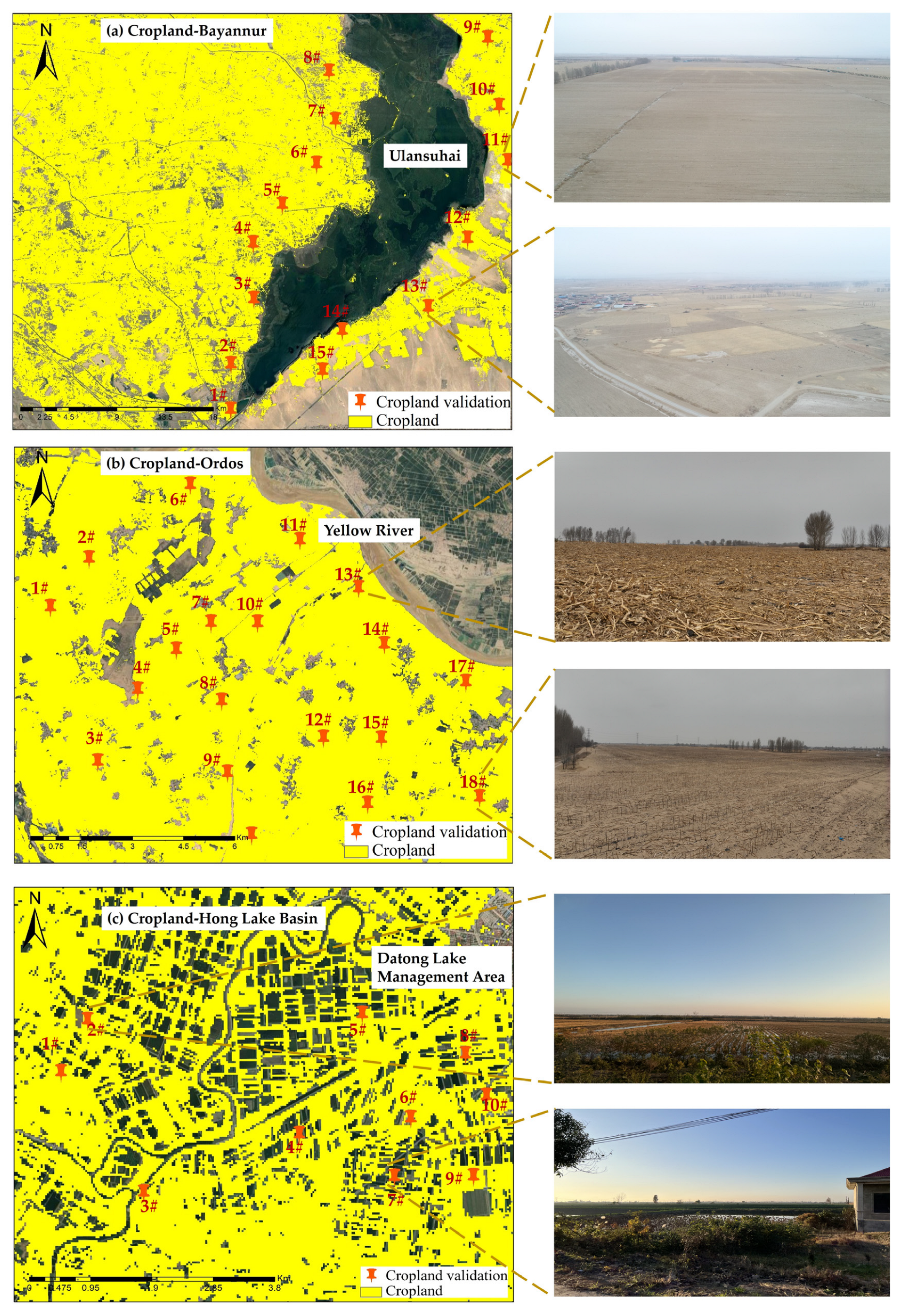
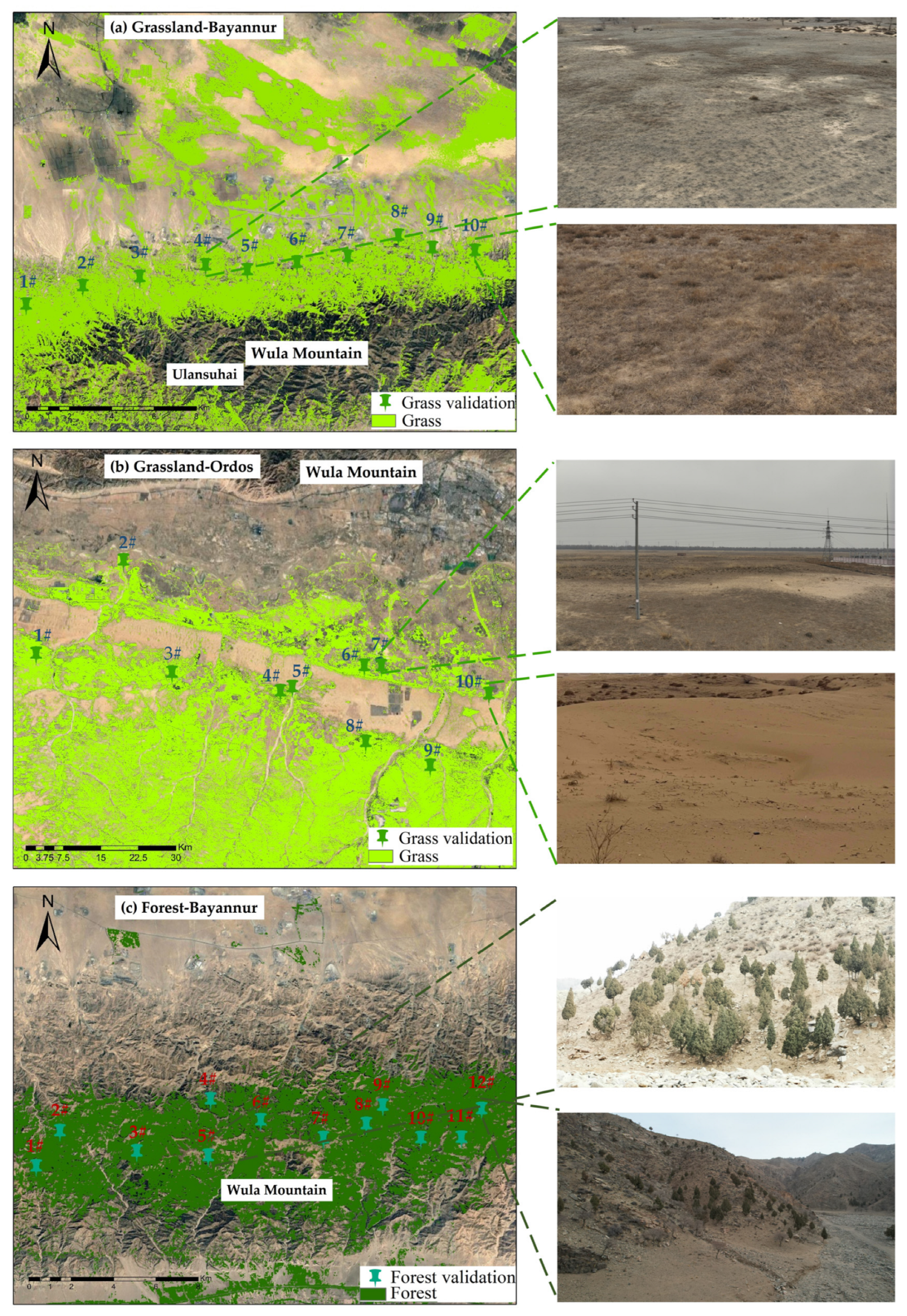
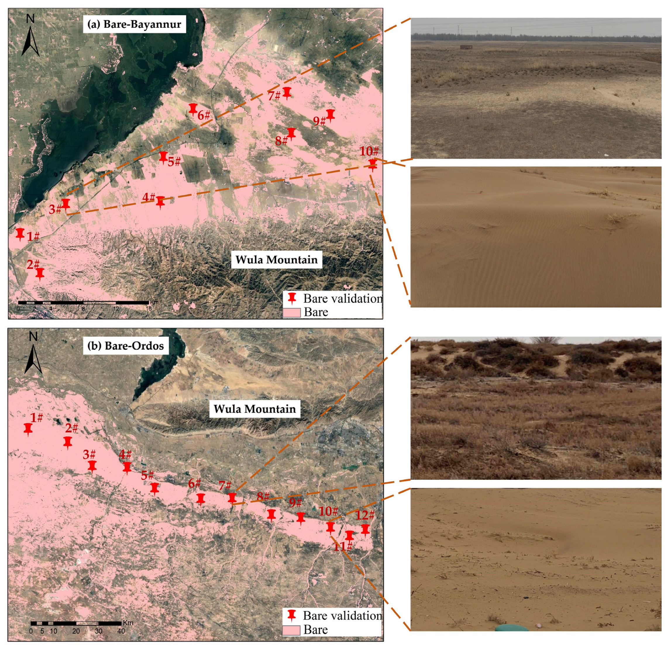
3.4. Field Validation
- (1)
- Cropland
- (2)
- Forest, grass and bare
- (3)
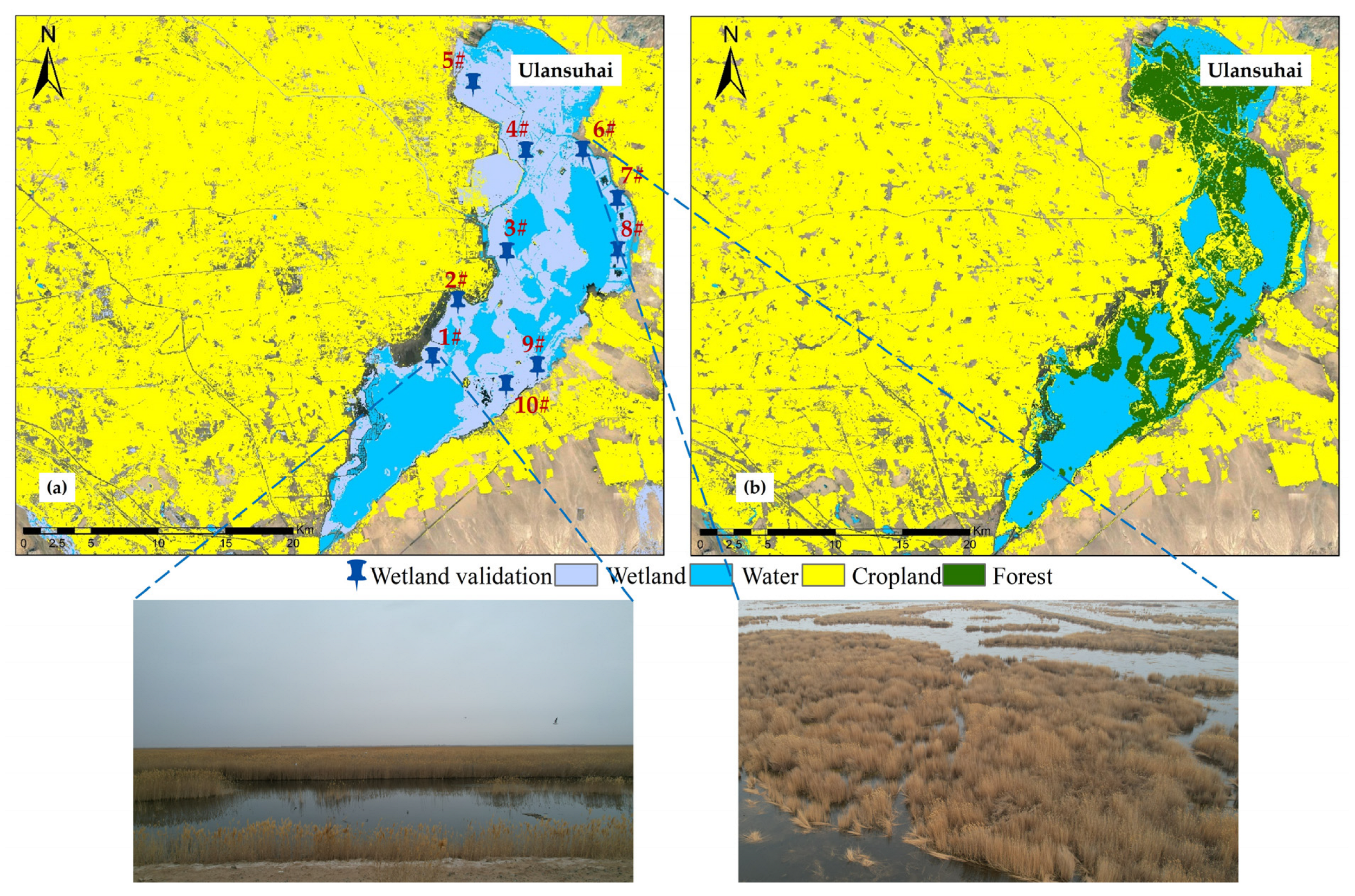
- Wetland
- (4)
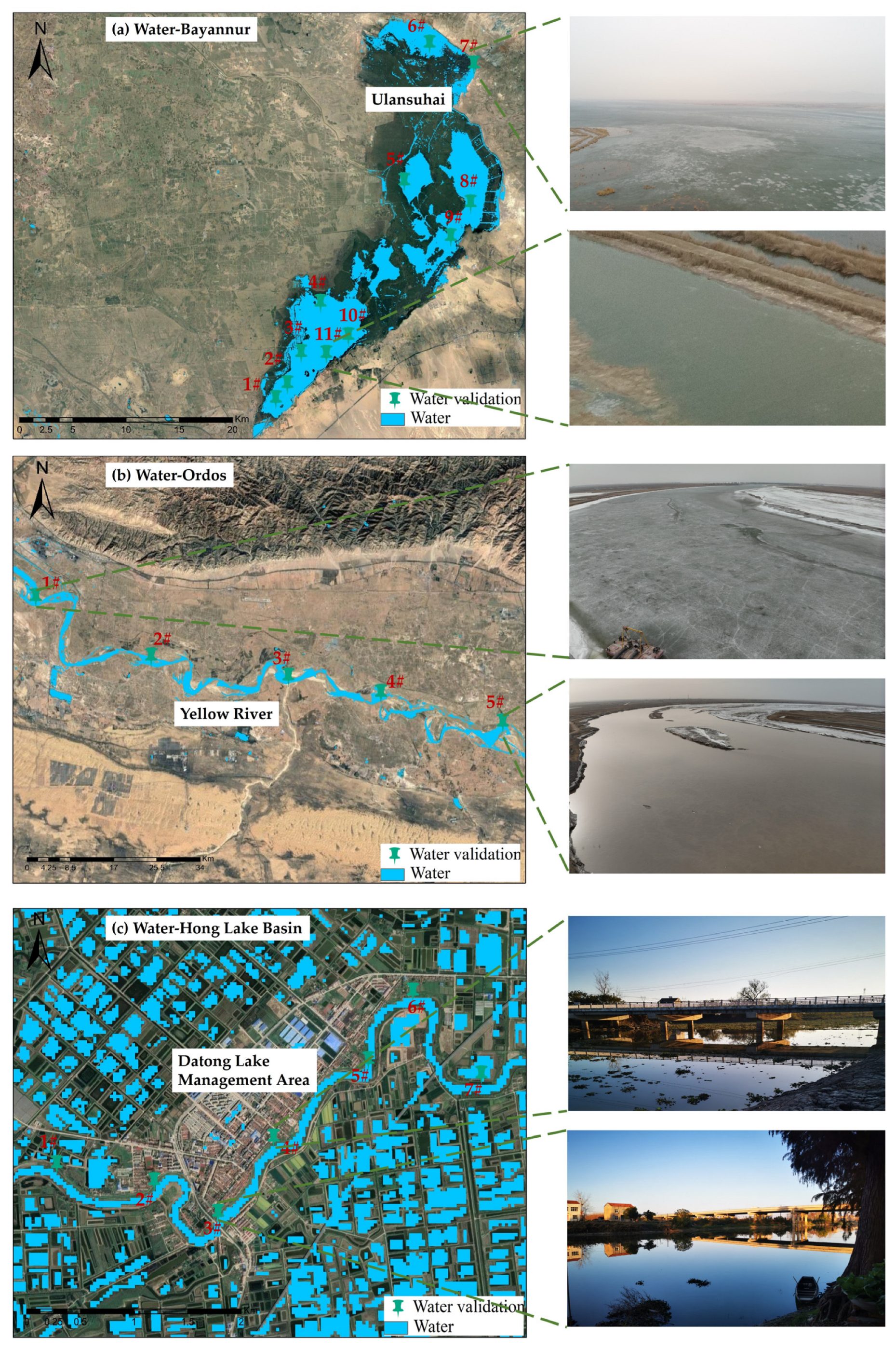
- Water
- (5)
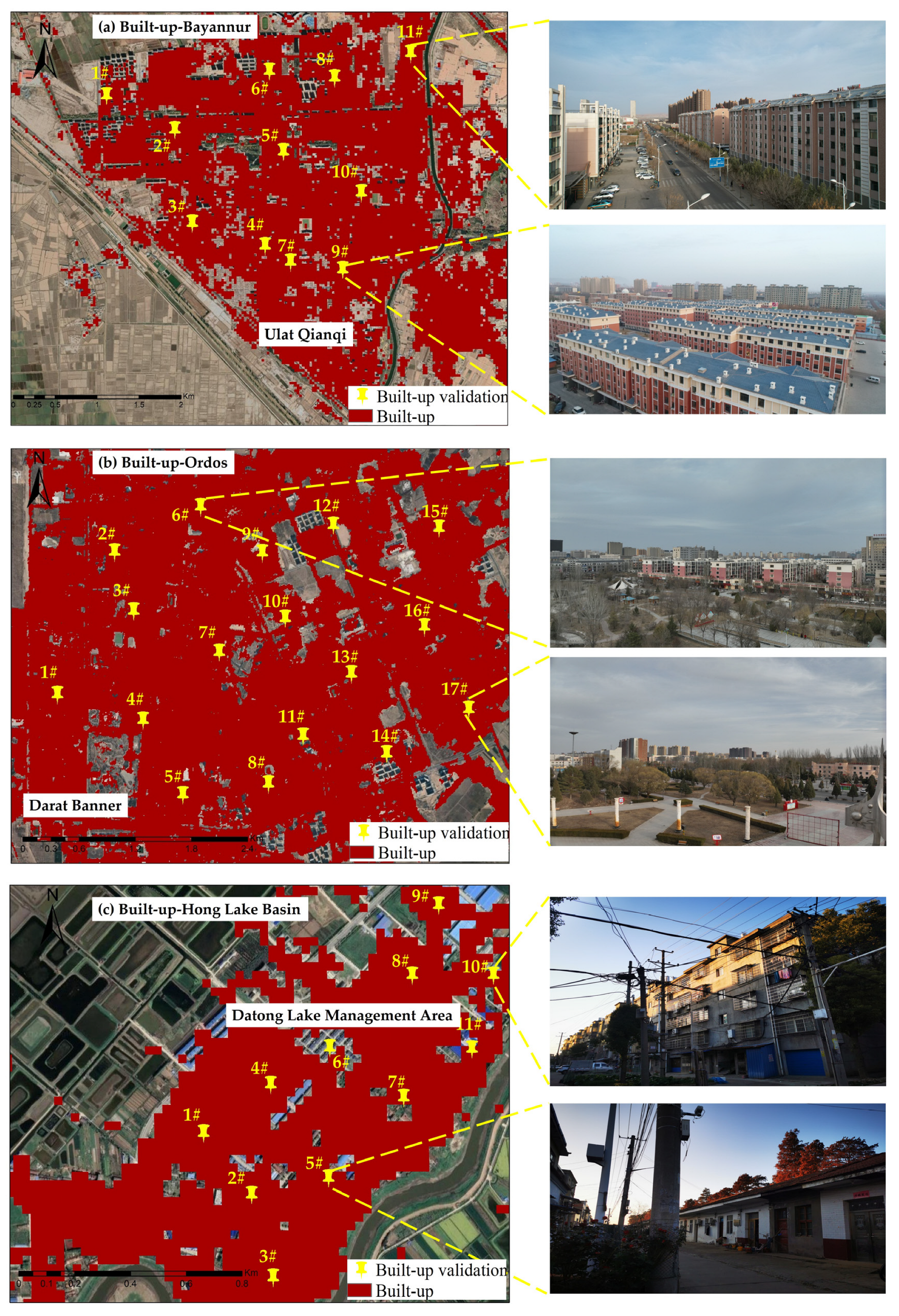
- Built-up
4. Discussion
4.1. Overcoming Land Use Classification Challenges
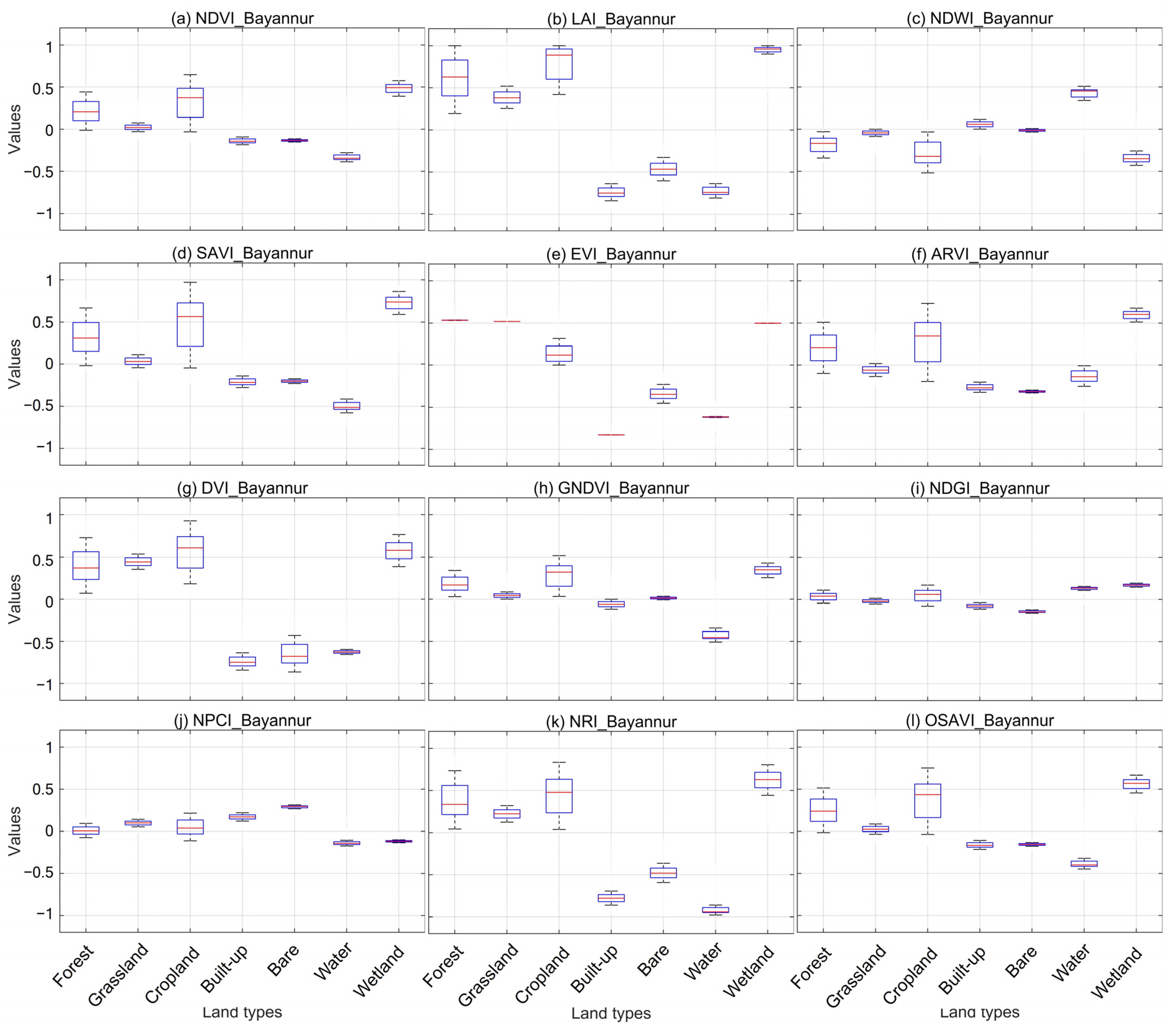
4.2. Spectral Indices for Data Augmentation
4.3. Limitations of Research
5. Conclusions
Author Contributions
Funding
Data Availability Statement
Conflicts of Interest
Abbreviations
| NDVI | Normalized Difference Vegetation Index |
| LAI | Leaf Area Index |
| SAVI | Source Address Validation Improvement |
| EVI | Enhanced Vegetation Index |
| ARVI | Atmospheric Resistance Vegetation Index |
| DVI | Difference Vegetation Index |
| GNDVI | Normalized Green Difference Vegetation Index |
| NDGI | Normalized Difference Green Degree Index |
| NPCI | Chorophyll Normalized Vegetation Index |
| NRI | Nitrogen Reflectance Index |
| OSAVI | Optimization Of Soil Regulatory Vegetation Index |
| MSAVI | Modified Soil Adjustment Vegetation Index |
| RVI | Ratio Vegetation Index |
| SIPI | Structure-Independent Pigment Index |
| TVI | Triangle Vegetation Index |
| VARI | Visible Atmospherically Resistant Index |
| WDRVI | Wide Dynamic Range Vegetation Index |
| CIVE | Vegetation Color Index |
| MSRI | Modified Second Ratio Index |
| NDWI | Normalized Difference Water Index |
| NDSI | Normalized Salinity Index |
| RBI | Ratio Built-up Index |
References
- Shi, K.; Liu, G.; Zhou, L.; Cui, Y.; Liu, S.; Wu, Y. Satellite remote sensing data reveal increased slope climbing of urban land expansion worldwide. Landsc. Urban Plan. 2023, 235, 104755. [Google Scholar] [CrossRef]
- Sun, Y.; Li, X.; Shi, H.; Cui, J.; Wang, W.; Ma, H.; Chen, N. Modeling salinized wasteland using remote sensing with the integration of decision tree and multiple validation approaches in Hetao irrigation district of China. Catena 2022, 209, 105854. [Google Scholar] [CrossRef]
- Zhang, W.; Huang, C.; Peng, H.; Wang, Y.; Zhao, Y.; Chen, T. Chlorophyll a (Chl-a) concentration measurement and prediction in Taihu lake based on MODIS image data. In Proceedings of the 8th International Symposium on Spatial Accuracy Assessment in Natural Resources and Environmental Sciences, Shanghai, China, 25–27 June 2008; pp. 352–359. [Google Scholar]
- Kafy, A.A.; Al Rakib, A.; Akter, K.S.; Jahir, D.M.A.; Sikdar, M.S.; Ashrafi, T.J.; Mallik, S.; Rahman, M.M. Assessing and predicting land use/land cover, land surface temperature and urban thermal field variance index using Landsat imagery for Dhaka Metropolitan area. Environ. Chall. 2021, 4, 100192. [Google Scholar]
- Pankaj, P.; Joseph, L.V.; Priyankar, C.; Mahender, K. Evaluation and comparison of the earth observing sensors in land cover/land use studies using machine learning algorithms. Ecol. Inform. 2021, 68, 101522. [Google Scholar]
- Curtis, P.G.; Slay, C.M.; Harris, N.L.; Tyukavina, A.; Hansen, M.C. Classifying drivers of global forest loss. Science 2018, 361, 1108–1111. [Google Scholar] [CrossRef]
- Evan, R.D.; Kariyeva, J.; Jason, T.B.; Jennifer, N.H. Large-scale probabilistic identification of boreal peatlands using Google Earth Engine, open-access satellite data, and machine learning. PLoS ONE 2019, 14, e0218165. [Google Scholar]
- Ludwig, C.; Walli, A.; Schleicher, C.; Weichselbaum, J.; Riffler, M. A highly automated algorithm for wetland detection using multi-temporal optical satellite data. Remote Sens. Environ. 2019, 224, 333–351. [Google Scholar] [CrossRef]
- Calderón-Loor, M.; Hadjikakou, M.; Bryan, B.A. High-resolution wall-to-wall land-cover mapping and land change assessment for Australia from 1985 to 2015. Remote Sens. Environ. 2021, 252, 112148. [Google Scholar] [CrossRef]
- Masolele, R.N.; De Sy, V.; Herold, M.; Marcos, D.; Verbesselt, J.; Gieseke, F.; Mullissa, A.G.; Martius, C. Spatial and temporal deep learning methods for deriving land-use following deforestation: A pan-tropical case study using Landsat time series. Remote Sens. Environ. 2021, 264, 112600. [Google Scholar] [CrossRef]
- Nguyen, L.H.; Joshi, D.R.; Clay, D.E.; Henebry, G.M. Characterizing land cover/land use from multiple years of Landsat and MODIS time series: A novel approach using land surface phenology modeling and random forest classifier. Remote Sens. Environ. 2018, 238, 111017. [Google Scholar] [CrossRef]
- Silva, A.L.; Alves, D.S.; Ferreira, M.P. Landsat-Based Land Use Change Assessment in the Brazilian Atlantic Forest: Forest Transition and Sugarcane Expansion. Remote Sens. 2018, 10, 996. [Google Scholar] [CrossRef]
- Xu, P.; Tsendbazar, N.E.; Herold, M.; Clevers, J.G.; Li, L. Improving the characterization of global aquatic land cover types using multi-source earth observation data. Remote Sens. Environ. 2022, 278, 113103. [Google Scholar] [CrossRef]
- Azedou, A.; Amine, A.; Kisekka, I.; Lahssini, S.; Bouziani, Y.; Moukrim, S. Enhancing Land Cover/Land Use (LCLU) classification through a comparative analysis of hyperparameters optimization approaches for deep neural network (DNN). Ecol. Inform. 2023, 78, 102333. [Google Scholar] [CrossRef]
- Li, P.; Feng, Z. Extent and Area of Swidden in Montane Mainland Southeast Asia: Estimation by Multi-Step Thresholds with Landsat-8 OLI Data. Remote Sens. 2016, 8, 44. [Google Scholar] [CrossRef]
- Yang, X.; Zhao, S.; Qin, X.; Zhao, N.; Liang, L. Mapping of Urban Surface Water Bodies from Sentinel-2 MSI Imagery at 10 m Resolution via NDWI-Based Image Sharpening. Remote Sens. 2017, 9, 596. [Google Scholar] [CrossRef]
- Li, K.; Chen, Y. A Genetic Algorithm-Based Urban Cluster Automatic Threshold Method by Combining VIIRS DNB, NDVI, and NDBI to Monitor Urbanization. Remote Sens. 2018, 10, 277. [Google Scholar] [CrossRef]
- Wang, Z.; Wang, X.; Zhang, Y.; Liao, Z.; Cai, J.; Yu, J. Estimation of a suitable NDVI oriented for ecological water savings and phytoremediation in Baiyangdian Lake, North China. Ecol. Indic. 2023, 148, 110030. [Google Scholar] [CrossRef]
- Li, C.; Song, Y.; Qin, T.; Yan, D.; Zhang, X.; Zhu, L.; Dorjsuren, B.; Khalid, H. Spatiotemporal Variations of Global Terrestrial Typical Vegetation EVI and Their Responses to Climate Change from 2000 to 2021. Remote Sens. 2023, 15, 4245. [Google Scholar] [CrossRef]
- Paz-Kagan, T.; Chang, J.G.; Shoshany, M.; Sternberg, M.; Karnieli, A. Assessment of plant species distribution and diversity along a climatic gradient from Mediterranean woodlands to semi-arid shrublands. GISci. Remote Sens. 2021, 58, 929–953. [Google Scholar] [CrossRef]
- Fu, Y.; Tan, X.; Yao, Y.; Wang, L.; Shan, Y.; Yang, Y.; Jing, Z. Uncovering optimal vegetation indices for estimating wetland plant species diversity. Ecol. Indic. 2024, 166, 112367. [Google Scholar] [CrossRef]
- Wang, Z.; Wang, J.; Wang, W.; Zhang, C.; Mandakh, U.; Ganbat, D.; Myanganbuu, N. An Explanation of the Differences in Grassland NDVI Change in the Eastern Route of the China–Mongolia–Russia Economic Corridor. Remote Sens. 2025, 17, 867. [Google Scholar] [CrossRef]
- Zhou, Y.; Lin, C.; Wang, S.; Liu, W.; Tian, Y. Estimation of Building Density with the Integrated Use of GF-1 PMS and Radarsat-2 Data. Remote Sens. 2016, 8, 969. [Google Scholar] [CrossRef]
- Allbed, A.; Kumar, L.; Aldakheel, Y.Y. Assessing soil salinity using soil salinity and vegetation indices derived from IKONOS high-spatial resolution imageries: Applications in a date palm dominated region. Geoderma 2014, 230–231, 1–8. [Google Scholar] [CrossRef]
- Xu, D.; An, D.; Guo, X. The Impact of Non-Photosynthetic Vegetation on LAI Estimation by NDVI in Mixed Grassland. Remote Sens. 2020, 12, 1979. [Google Scholar] [CrossRef]
- Qiao, K.; Zhu, W.; Xie, Z.; Wu, S.; Li, S. New three red-edge vegetation index (VI3RE) for crop seasonal LAI prediction using Sentinel-2 data. Int. J. Appl. Earth Obs. Geoinf. 2024, 130, 103894. [Google Scholar] [CrossRef]
- Huang, X.; Lin, D.; Mao, X.; Zhao, Y. Multi-source data fusion for estimating maize leaf area index over the whole growing season under different mulching and irrigation conditions. Field Crops Res. 2023, 303, 109111. [Google Scholar] [CrossRef]
- Ren, H.; Zhou, G.; Zhang, F. Using negative soil adjustment factor in soil-adjusted vegetation index (SAVI) for aboveground living biomass estimation in arid grasslands. Remote Sens. Environ. 2018, 209, 439–445. [Google Scholar] [CrossRef]
- Nyamtseren, M.; Pham, T.D.; Vu, T.T.P.; Navaandorj, I.; Shoyama, K. Mapping Vegetation Changes in Mongolian Grasslands (1990–2024) Using Landsat Data and Advanced Machine Learning Algorithm. Remote Sens. 2025, 17, 400. [Google Scholar] [CrossRef]
- Raza, A.; Shahid, M.A.; Zaman, M.; Miao, Y.; Huang, Y.; Safdar, M.; Maqbool, S.; Muhammad, N.E. Improving Wheat Yield Prediction with Multi-Source Remote Sensing Data and Machine Learning in Arid Regions. Remote Sens. 2025, 17, 774. [Google Scholar] [CrossRef]
- Wang, Q.; Pang, Y.; Li, Z.; Sun, G.; Chen, E.; Ni-Meister, W. The Potential of Forest Biomass Inversion Based on Vegetation Indices Using Multi-Angle CHRIS/PROBA Data. Remote Sens. 2016, 8, 891. [Google Scholar] [CrossRef]
- Qian, D.; Li, Q.; Fan, B.; Zhou, H.; Du, Y.; Guo, X. Spectral Characteristics and Identification of Degraded Alpine Meadow in Qinghai–Tibetan Plateau Based on Hyperspectral Data. Remote Sens. 2024, 16, 3884. [Google Scholar] [CrossRef]
- Taylor-Zavala, R.; Ramírez-Rodríguez, O.; de Armas-Ricard, M.; Sanhueza, H.; Higueras-Fredes, F.; Mattar, C. Quantifying Biochemical Traits over the Patagonian Sub-Antarctic Forests and Their Relation to Multispectral Vegetation Indices. Remote Sens. 2021, 13, 4232. [Google Scholar] [CrossRef]
- Pastor-Guzman, J.; Dash, J.; Atkinson, P.M. Remote sensing of mangrove forest phenology and its environmental drivers. Remote Sens. Environ. 2018, 205, 71–84. [Google Scholar] [CrossRef]
- Wavrek, M.T.; Carr, E.; Jean-Philippe, S.; McKinney, M.L. Drone remote sensing in urban forest management: A case study. Urban For. Urban Green. 2023, 86, 127978. [Google Scholar] [CrossRef]
- Rezaei, R.; Ghaffarian, S. Monitoring Forest Resilience Dynamics from Very High-Resolution Satellite Images in Case of Multi-Hazard Disaster. Remote Sens. 2021, 13, 4176. [Google Scholar] [CrossRef]
- Cao, Y.; Li, G.L.; Luo, Y.K.; Pan, Q.; Zhang, S.Y. Monitoring of sugar beet growth indicators using wide-dynamic-range vegetation index (WDRVI) derived from UAV multispectral images. Comput. Electron. Agric. 2020, 171, 105331. [Google Scholar] [CrossRef]
- Testa, S.; Soudani, K.; Boschetti, L.; Mondino, E.B. MODIS-derived EVI, NDVI and WDRVI time series to estimate phenological metrics in French deciduous forests. Int. J. Appl. Earth Obs. Geoinf. 2018, 64, 132–144. [Google Scholar] [CrossRef]
- Hamada, Y.; Szoldatits, K.; Grippo, M.; Hartmann, H.M. Remotely Sensed Spatial Structure as an Indicator of Internal Changes of Vegetation Communities in Desert Landscapes. Remote Sens. 2019, 11, 1495. [Google Scholar] [CrossRef]
- Änäkkälä, M.; Lajunen, A.; Hakojärvi, M.; Alakukku, L. Evaluation of the Influence of Field Conditions on Aerial Multispectral Images and Vegetation Indices. Remote Sens. 2022, 14, 4792. [Google Scholar] [CrossRef]
- Gao, S.; Yan, K.; Liu, J.; Pu, J.; Zou, D.; Qi, J.; Mu, X.; Yan, G. Assessment of remote-sensed vegetation indices for estimating forest chlorophyll concentration. Ecol. Indic. 2024, 162, 112001. [Google Scholar] [CrossRef]
- Dye, D.G.; Middleton, B.R.; Vogel, J.M.; Wu, Z.; Velasco, M. Exploiting Differential Vegetation Phenology for Satellite-Based Mapping of Semiarid Grass Vegetation in the Southwestern United States and Northern Mexico. Remote Sens. 2016, 8, 889. [Google Scholar] [CrossRef]
- He, S.; Shao, H.; Xian, W.; Zhang, S.; Zhong, J.; Qi, J. Extraction of Abandoned Land in Hilly Areas Based on the Spatio-Temporal Fusion of Multi-Source Remote Sensing Images. Remote Sens. 2021, 13, 3956. [Google Scholar] [CrossRef]
- Fern, R.R.; Foxley, E.A.; Bruno, A.; Morrison, M.L. Suitability of NDVI and OSAVI as estimators of green biomass and coverage in a semi-arid rangeland. Ecol. Indic. 2018, 94, 16–21. [Google Scholar] [CrossRef]
- Li, J.; Meng, Y.; Li, Y.; Cui, Q.; Yang, X.; Tao, C.; Wang, Z.; Li, L.; Zhang, W. Accurate water extraction using remote sensing imagery based on normalized difference water index and unsupervised deep learning. J. Hydrol. 2022, 612, 128202. [Google Scholar] [CrossRef]
- Worden, J.; de Beurs, K.M. Surface water detection in the Caucasus. Int. J. Appl. Earth Obs. Geoinf. 2020, 91, 102159. [Google Scholar] [CrossRef]
- Cheng, Y.; Zhang, W.; Wang, H.; Wang, X. Causal Meta-Transfer Learning for Cross-Domain Few-Shot Hyperspectral Image Classification. IEEE Trans. Geosci. Remote Sens. 2023, 61, 5521014. [Google Scholar] [CrossRef]
- Christopher, F.B.; Steven, P.B.; Williams, B.G.; Birch, T.; Samantha, B.H.; Mazzariello, J.; Czerwinski, W.; Valerie, J.P.; Haertel, R.; Ilyushchenko, S.; et al. Dynamic World, Near real-time global 10 m land use land cover mapping. Sci. Data 2022, 9, 251. [Google Scholar]
- Garg, R.; Kumar, A.; Bansal, N.; Prateek, M.; Kumar, S. Semantic segmentation of PolSAR image data using advanced deep learning model. Sci. Rep. 2021, 11, 15365. [Google Scholar] [CrossRef]
- Li, Y.; Zhang, H.; Xue, X.; Jiang, Y.; Shen, Q. Deep learning for remote sensing image classification: A survey. Wiley Interdiscip. Rev. Data Min. Knowl. Discov. 2018, 8, e1264. [Google Scholar] [CrossRef]
- Li, Z.; He, W.; Cheng, M.; Hu, J.; Yang, G.; Zhang, H. SinoLC-1: The first 1 m resolution national-scale land-cover map of China created with a deep learning framework and open-access data. Earth Syst. Sci. Data 2023, 15, 4749–4780. [Google Scholar] [CrossRef]
- Yuan, Q.; Shen, H.; Li, T.; Li, Z.; Li, S.; Jiang, Y.; Xu, H.; Tan, W.; Yang, Q.; Wang, J.; et al. Deep learning in environmental remote sensing: Achievements and challenges. Remote Sens. Environ. 2020, 241, 111716. [Google Scholar] [CrossRef]
- Huang, B.; Zhao, B.; Song, Y. Urban land-use mapping using a deep convolutional neural network with high spatial resolution multispectral remote sensing imagery. Remote Sens. Environ. 2018, 214, 73–86. [Google Scholar] [CrossRef]
- Ansith, S.; Bini, A.A. Land use classification of high-resolution remote sensing images using an encoder based modified GAN architecture. Displays 2022, 74, 102229. [Google Scholar]
- Scheibenreif, L.; Hanna, J.; Mommert, M.; Borth, D. Self-supervised Vision Transformers for Land-cover Segmentation and Classification. In Proceedings of the IEEE/CVF Conference on Computer Vision and Pattern Recognition Workshops (CVPRW), New Orleans, LA, USA, 19–20 June 2022; pp. 1421–1430. [Google Scholar]
- Xiao, B.; Liu, J.; Jiao, J.; Li, Y.; Liu, X.; Zhu, W. Modeling dynamic land use changes in the eastern portion of the hexi corridor, China by cnn-gru hybrid model. GISci. Remote Sens. 2022, 59, 501–519. [Google Scholar] [CrossRef]
- Kussul, N.; Lavreniuk, M.; Skakun, S.; Shelestov, A. Deep Learning Classification of Land Cover and Crop Types Using Remote Sensing Data. IEEE Geosci. Remote Sens. Lett. 2017, 14, 778–782. [Google Scholar] [CrossRef]
- Maggiori, E.; Tarabalka, Y.; Charpiat, G.; Alliez, P. Convolutional Neural Networks for Large-Scale Remote-Sensing Image Classification. IEEE Trans. Geosci. Remote Sens. 2017, 55, 645–657. [Google Scholar] [CrossRef]
- Volpi, M.; Tuia, D. Dense Semantic Labeling of Subdecimeter Resolution Images with Convolutional Neural Networks. IEEE Trans. Geosci. Remote Sens. 2017, 55, 881–893. [Google Scholar] [CrossRef]
- Zhang, C.; Pan, X.; Li, H.; Gardiner, A.; Sargent, I.; Hare, J.; Atkinson, P.M. A hybrid MLP-CNN classifier for very fine resolution remotely sensed image classification. ISPRS-J. Photogramm. Remote Sens. 2018, 140, 133–144. [Google Scholar] [CrossRef]
- Tong, X.; Xia, G.; Lu, Q.; Shen, H.; Li, S.; You, S.; Zhang, L. Land-cover classification with high-resolution remote sensing images using transferable deep models. Remote Sens. Environ. 2020, 237, 111322. [Google Scholar] [CrossRef]
- LeCun, Y.; Bengio, Y.; Hinton, G. Deep learning. Nature 2015, 521, 436–444. [Google Scholar] [CrossRef]
- Hu, F.; Xia, G.; Hu, J.; Zhang, L. Transferring Deep Convolutional Neural Networks for the Scene Classification of High-Resolution Remote Sensing Imagery. Remote Sens. 2015, 7, 14680–14707. [Google Scholar] [CrossRef]
- Xu, G.; Zhu, X.; Fu, D.; Dong, J.; Xiao, X. Automatic land cover classification of geo-tagged field photos by deep learning. Environ. Model. Softw. 2017, 91, 127–134. [Google Scholar] [CrossRef]
- Zhu, X.X.; Tuia, D.; Mou, L.; Xia, G.S.; Zhang, L.; Xu, F.; Fraundorfer, F. Deep Learning in Remote Sensing: A Comprehensive Review and List of Resources. IEEE Geosci. Remote Sens. Mag. 2017, 5, 8–36. [Google Scholar] [CrossRef]
- Krizhevsky, A.; Sutskever, I.; Hinton, G.E. ImageNet classification with deep convolutional neural networks. Commun. ACM 2017, 60, 84–90. [Google Scholar] [CrossRef]
- Marmanis, D.; Datcu, M.; Esch, T.; Stilla, U. Deep Learning Earth Observation Classification Using ImageNet Pretrained Networks. IEEE Geosci. Remote Sens. Lett. 2016, 13, 105–109. [Google Scholar] [CrossRef]
- Zhao, B.; Huang, B.; Zhong, Y. Transfer Learning with Fully Pretrained Deep Convolution Networks for Land-Use Classification. IEEE Geosci. Remote Sens. Lett. 2017, 14, 1436–1440. [Google Scholar] [CrossRef]
- Li, Z.; Chen, B.; Wu, S.; Su, M.; Chen, J.M.; Xu, B. Deep learning for urban land use category classification: A review and experimental assessment. Remote Sens. Environ. 2024, 311, 114290. [Google Scholar] [CrossRef]
- Feng, B.; Liu, Y.; Chi, H.; Chen, X. Hyperspectral remote sensing image classification based on residual generative Adversarial Neural Networks. Signal Process. 2023, 213, 109202. [Google Scholar] [CrossRef]
- Zhang, B.; Zhao, L.; Zhang, X. Three-dimensional convolutional neural network model for tree species classification using airborne hyperspectral images. Remote Sens. Environ. 2020, 247, 111938. [Google Scholar] [CrossRef]
- Dong, W.; Lan, J.; Liang, S.; Yao, W.; Zhan, Z. Selection of LiDAR geometric features with adaptive neighborhood size for urban land cover classification. Int. J. Appl. Earth Obs. Geoinf. 2017, 60, 99–110. [Google Scholar] [CrossRef]
- Kriegler, F.J.; Malila, W.A.; Nalepka, R.F.; Richardson, W. Preprocessing Transformations and Their Effects on Multispectral Recognition. In Proceedings of the 6th International Symposium on Remote Sensing of Environment, Ann Arbor, MI, USA, 13–16 October 1969. [Google Scholar]
- Marks, P.L.; Bormann, F.H. Revegetation following Forest Cutting: Mechanisms for Return to Steady-State Nutrient Cycling. Science 1972, 176, 914–915. [Google Scholar] [CrossRef] [PubMed]
- Huete, A.R. A soil-adjusted vegetation index (SAVI). Remote Sens. Environ. 1988, 25, 295–309. [Google Scholar] [CrossRef]
- Miura, T.; Huete, A.R.; Yoshioka, H. Evaluation of sensor calibration uncertainties on vegetation indices for MODIS. IEEE Trans. Geosci. Remote Sen. 2000, 38, 1399–1409. [Google Scholar] [CrossRef]
- Kaufman, Y.J.; Tanre, D. Atmospherically resistant vegetation index (ARVI) for EOS-MODIS. IEEE Trans. Geosci. Remote Sens. 1992, 30, 261–270. [Google Scholar] [CrossRef]
- Richardsons, A.J.; Wiegand, A. Distinguishing vegetation from soil background information. Photogramm. Eng. Remote Sens. 1977, 43, 1541–1552. [Google Scholar]
- Daughtry, C.S.T.; Gallo, K.P.; Goward, S.N.; Prince, S.D.; Kustas, W.P. Spectral estimates of absorbed radiation and phytomass production in corn and soybean canopies. Remote Sens. Environ. 1992, 39, 141–152. [Google Scholar] [CrossRef]
- Lyon, J.G.; Yuan, D.; Lunetta, R.; Elvidge, C.D. A change detection experiment using vegetation indices. Photogramm. Eng. Remote Sens. 1998, 64, 143–150. [Google Scholar]
- Clay, D.E.; Kim, K.; Chang, J.; Clay, S.A.; Dalsted, K. Characterizing Water and Nitrogen Stress in Corn Using Remote Sensing. Agron. J. 2006, 98, 579–587. [Google Scholar] [CrossRef]
- Diker, K.; Bausch, W.C. Potential Use of Nitrogen Reflectance Index to estimate Plant Parameters and Yield of Maize. Biosyst. Eng. 2003, 85, 437–447. [Google Scholar] [CrossRef]
- Rondeaux, G.; Steven, M.; Baret, F. Optimization of soil-adjusted vegetation indices. Remote Sens. Environ. 1996, 55, 95–107. [Google Scholar] [CrossRef]
- Qi, J.; Chehbouni, A.; Huete, A.R.; Kerr, Y.H.; Sorooshian, S. A modified soil adjusted vegetation index. Remote Sens. Environ. 1994, 48, 119–126. [Google Scholar] [CrossRef]
- Pearson, R.L.; Miller, L.D. Remote Mapping of Standing Crop Biomass for Estimation of Productivity of the Shortgrass Prairie. In Proceedings of the Eighth International Symposium on Remote Sensing of Environment, Ann Arbor, MI, USA, 2–6 October 1972. [Google Scholar]
- Penuelas, J.; Baret, F.; Filella, I. Semiempirical Indexes to Assess Carotenoids Chlorophyll-a Ratio from Leaf Spectral Reflectance. Photosynthetica 1995, 31, 221–230. [Google Scholar]
- Rouse, J.W.; Haas, R.H.; Deering, D.W.; Schell, J.A.; Harlan, J.C. Monitoring the Vernal Advancement and Retrogradation (Green Wave Effect) of Natural Vegetation; NASA: Washington, DC, USA, 1973.
- Gitelson, A.A.; Kaufman, Y.J.; Stark, R.; Rundquist, D. Novel algorithms for remote estimation of vegetation fraction. Remote Sens. Environ. 2002, 80, 76–87. [Google Scholar] [CrossRef]
- Gitelson, A.A. Wide Dynamic Range Vegetation Index for Remote Quantification of Biophysical Characteristics of Vegetation. J. Plant Physiol. 2004, 161, 165–173. [Google Scholar] [CrossRef]
- Huete, A.R.; Liu, H.; de Lira, G.R.; Batchily, K.; Escadafal, R. A soil color index to adjust for soil and litter noise in vegetation index imagery of arid regions. In Proceedings of the IGARSS’94-1994 IEEE International Geoscience and Remote Sensing Symposium, Pasadena, CA, USA, 8–12 August 1994; pp. 1042–1043. [Google Scholar]
- Chen, J.M.; Cihlar, J. Retrieving leaf area index of boreal conifer forests using Landsat TM images. Remote Sens. Environ. 1996, 55, 153–162. [Google Scholar] [CrossRef]
- Gao, B. NDWI—A normalized difference water index for remote sensing of vegetation liquid water from space. Remote Sens. Environ. 1996, 58, 257–266. [Google Scholar] [CrossRef]
- Khan, N.M.; Rastoskuev, V.V.; Sato, Y.; Shiozawa, S. Assessment of hydrosaline land degradation by using a simple approach of remote sensing indicators. Agric. Water Manag. 2005, 77, 96–109. [Google Scholar] [CrossRef]
- Wang, J.; Yang, D.; Chen, S.; Zhu, X.; Wu, S.; Bogonovich, M.; Guo, Z.; Zhu, Z.; Wu, J. Automatic cloud and cloud shadow detection in tropical areas for PlanetScope satellite images. Remote Sens. Environ. 2021, 264, 112604. [Google Scholar] [CrossRef]
- Zhu, Z.; Woodcock, C.E. Object-based cloud and cloud shadow detection in Landsat imagery. Remote Sens. Environ. 2012, 118, 83–94. [Google Scholar] [CrossRef]
- Zhu, X.; Helmer, E.H. An automatic method for screening clouds and cloud shadows in optical satellite image time series in cloudy regions. Remote Sens. Environ. 2018, 214, 135–153. [Google Scholar] [CrossRef]
- Landis, J.R.; Koch, G.G. The measurement of observer agreement for categorical data. Biometrics 1977, 33, 159–174. [Google Scholar] [CrossRef] [PubMed]
- Pan, S.; Guan, H.; Chen, Y.; Yu, Y.; Gonçalves, W.N.; Junior, J.M.; Li, J. Land-cover classification of multispectral LiDAR data using CNN with optimized hyper-parameters. ISPRS-J. Photogramm. Remote Sens. 2020, 166, 241–254. [Google Scholar] [CrossRef]
- Kwan, C.; Ayhan, B.; Budavari, B.; Lu, Y.; Perez, D.; Li, J.; Bernabe, S.; Plaza, A. Deep Learning for Land Cover Classification Using Only a Few Bands. Remote Sens. 2020, 12, 2000. [Google Scholar] [CrossRef]
- Fromm, L.T.; Smith, L.C.; Kyzivat, E.D. Wetland vegetation mapping improved by phenological leveraging of multitemporal nanosatellite images. Geocarto Int. 2025, 40, 2452252. [Google Scholar] [CrossRef]
- As-syakur, A.R.; Adnyana, I.W.S.; Arthana, I.W.; Nuarsa, I.W. Enhanced Built-Up and Bareness Index (EBBI) for Mapping Built-Up and Bare Land in an Urban Area. Remote Sens. 2012, 4, 2957–2970. [Google Scholar] [CrossRef]
- Ettehadi Osgouei, P.; Kaya, S.; Sertel, E.; Alganci, U. Separating Built-Up Areas from Bare Land in Mediterranean Cities Using Sentinel-2A Imagery. Remote Sens. 2019, 11, 345. [Google Scholar] [CrossRef]
- Che, L.; Li, S.; Liu, X. Improved surface water mapping using satellite remote sensing imagery based on optimization of the Otsu threshold and effective selection of remote-sensing water index. J. Hydrol. 2025, 654, 132771. [Google Scholar] [CrossRef]
- Fisher, A.; Flood, N.; Danaher, T. Comparing Landsat water index methods for automated water classification in eastern Australia. Remote Sens. Environ. 2016, 175, 167–182. [Google Scholar] [CrossRef]
- Binding, C.E.; Bowers, D.G.; Mitchelson-Jacob, E.G. Estimating suspended sediment concentrations from ocean colour measurements in moderately turbid waters; the impact of variable particle scattering properties. Remote Sens. Environ. 2005, 94, 373–383. [Google Scholar] [CrossRef]

| Index | Variable and Reference |
|---|---|
| Vegetation | NDVI [73] |
| LAI [74] | |
| SAVI [75] | |
| EVI [76] | |
| ARVI [77] | |
| DVI [78] | |
| GNDVI [79] | |
| NDGI [80] | |
| NPCI [81] | |
| NRI [82] | |
| OSAVI [83] | |
| MSAVI [84] | |
| RVI [85] | |
| SIPI [86] | |
| TVI [87] | |
| VARI [88] | |
| WDRVI [89] | |
| CIVE [90] | |
| MSRI [91] | |
| Water | NDWI [92] |
| Soil | NDSI [93] |
| RBI [23] |
| ID | Land Use | Bayannur | Ordos | Hong Lake Basin | ||||||
|---|---|---|---|---|---|---|---|---|---|---|
| Precision | Recall | F1-Score | Precision | Recall | F1-Score | Precision | Recall | F1-Score | ||
| 1 | Forest | 99.09% | 98.71% | 0.98898 | 81.08% | 76.92% | 0.78947 | - | - | - |
| 2 | Grassland | 98.38% | 98.29% | 0.98333 | 93.11% | 98.59% | 0.95771 | - | - | - |
| 3 | Cropland | 99.09% | 99.52% | 0.99306 | 100.00% | 87.10% | 0.93103 | 79.80% | 93.07% | 0.85925 |
| 4 | Built-up | 99.27% | 98.28% | 0.98773 | 96.21% | 94.00% | 0.95094 | 93.28% | 92.24% | 0.92756 |
| 5 | Bare | 99.96% | 99.99% | 0.99972 | 98.50% | 100.00% | 0.99242 | 96.97% | 85.70% | 0.90987 |
| 6 | Water | 99.73% | 99.73% | 0.99733 | 93.58% | 87.18% | 0.90265 | - | - | - |
| 7 | Wetland | 99.44% | 99.38% | 0.99409 | - | - | - | - | - | - |
| Macro-average | 99.28% | 99.13% | 0.99203 | 93.75% | 90.63% | 0.92071 | 90.01% | 90.34% | 0.89890 | |
| Land Use | Verification Point | Errors | Accuracy (%) |
|---|---|---|---|
| Built-up | 39 | 0 | 100.00 |
| Cropland | 41 | 0 | 100.00 |
| Grass | 18 | 1 | 94.44 |
| Forest | 12 | 0 | 100.00 |
| Bare | 22 | 2 | 90.91 |
| Water | 23 | 0 | 100.00 |
| Wetland | 10 | 0 | 100.00 |
| Overall accuracy (%) | 98.18 | ||
Disclaimer/Publisher’s Note: The statements, opinions and data contained in all publications are solely those of the individual author(s) and contributor(s) and not of MDPI and/or the editor(s). MDPI and/or the editor(s) disclaim responsibility for any injury to people or property resulting from any ideas, methods, instructions or products referred to in the content. |
© 2025 by the authors. Licensee MDPI, Basel, Switzerland. This article is an open access article distributed under the terms and conditions of the Creative Commons Attribution (CC BY) license (https://creativecommons.org/licenses/by/4.0/).
Share and Cite
Wang, Y.; Zhang, W.; Liu, X.; Peng, H.; Lin, M.; Li, A.; Jiang, A.; Ma, N.; Wang, L. A Deep Learning Method for Land Use Classification Based on Feature Augmentation. Remote Sens. 2025, 17, 1398. https://doi.org/10.3390/rs17081398
Wang Y, Zhang W, Liu X, Peng H, Lin M, Li A, Jiang A, Ma N, Wang L. A Deep Learning Method for Land Use Classification Based on Feature Augmentation. Remote Sensing. 2025; 17(8):1398. https://doi.org/10.3390/rs17081398
Chicago/Turabian StyleWang, Yue, Wanshun Zhang, Xin Liu, Hong Peng, Minbo Lin, Ao Li, Anna Jiang, Ning Ma, and Lu Wang. 2025. "A Deep Learning Method for Land Use Classification Based on Feature Augmentation" Remote Sensing 17, no. 8: 1398. https://doi.org/10.3390/rs17081398
APA StyleWang, Y., Zhang, W., Liu, X., Peng, H., Lin, M., Li, A., Jiang, A., Ma, N., & Wang, L. (2025). A Deep Learning Method for Land Use Classification Based on Feature Augmentation. Remote Sensing, 17(8), 1398. https://doi.org/10.3390/rs17081398