Article

Formal Quantification of Spatially Differential Characteristics of PSI-Derived Vertical Surface Deformation Using Regular Triangle Network: A Case Study of Shixi in the Northwest Xuzhou Coalfield

1
Jiangsu Geological Bureau, Nanjing 210018, China
2
State Key Laboratory of Resources and Environmental Information System, Institute of Geographic Sciences and Natural Resources Research, Chinese Academy of Sciences, Beijing 100101, China
3
University of Chinese Academy of Sciences, Beijing 100049, China
4
College of Earth Science and Engineering, Shandong University of Science and Technology, Qingdao 266590, China
*
Author to whom correspondence should be addressed.
Remote Sens. 2025, 17(8), 1388; https://doi.org/10.3390/rs17081388
Submission received: 15 January 2025 / Revised: 1 April 2025 / Accepted: 11 April 2025 / Published: 14 April 2025
(This article belongs to the Special Issue Machine Learning for Spatiotemporal Remote Sensing Data (2nd Edition))

Abstract

:
This study addresses the challenge of quantifying spatially differential vertical surface deformation (SDVSD). Traditional approaches using persistent scatterer interferometry (PSI) data often focus on bulk vertical surface deformation (VSD) but overlook directional variability and struggle with irregularly distributed persistent scatterer (PS) points, limiting comprehensive SDVSD analysis. This study proposes a regular triangle network (RTN)-based framework that tessellates the study area into uniform triangular units, enabling the systematic quantification of the SDVSD direction, magnitude and rate while mitigating spatial biases from uneven PS distributions. Applied to the Shixi area in China’s Northwest Xuzhou Coalfield, the RTN-based framework revealed that (1) the SDVSD directionality aligned with the coal strata dip and working face distribution, contrasting with VSD’s focus on the magnitude and rate alone; (2) SDVSD exhibited seasonal rate fluctuations suggesting environmental influences, and, unlike VSD, it has a non-additivity property in temporal evolution; (3) there was spatial divergence between SDVSD and VSD, i.e., high VSD rates did not necessarily correlate with high SDVSD rates, emphasizing the need for an independent spatial gradient analysis. This study demonstrates that the RTN-based framework effectively disentangles the directional and magnitude (rate) components of SDVSD, offering a robust tool for the identification of deformation hotspots and linking surface dynamics to subsurface processes. By formalizing the quantification of PSI-derived SDVSD, this study advances InSAR deformation monitoring, providing actionable insights for infrastructure risk mitigation and sustainable land management in mining regions and beyond.

1. Introduction

Spatially differential vertical surface deformation (SDVSD) describes the spatial heterogeneity of the Earth’s vertical surface displacement (either subsidence or uplift in the vertical direction), i.e., it refers to the uneven or non-uniform sinking or rising of the land surface [1,2,3,4,5,6]. Unlike spatially uniform or quasi-uniform vertical surface deformation (VSD), which reflects the bulk displacement over a region, SDVSD emphasizes localized gradients, such as abrupt changes in VSD rates within the spatial domain. This phenomenon often occurs in regions where the subsurface conditions, such as rock–soil types, groundwater levels, or human activities, vary significantly over relatively short distances [7,8,9,10]. SDVSD can lead to structural damage on the surface, impacting natural environments and infrastructure [11,12,13,14]. Globally, SDVSD has posed severe hazards. For example, SDVSD in coalfields manifests as irregular ground fissures, infrastructure tilting, and residential collapses due to uneven stress redistribution after mining [15,16]; similarly, differential subsidence induced by groundwater extraction has damaged aqueducts and roads [17,18]. Such cases highlight the need for SDVSD monitoring and characterization to mitigate infrastructure risks and environmental degradation.
Interferometric synthetic aperture radar (InSAR), particularly time series InSAR, has become an essential tool in monitoring surface deformation due to its ability to provide data with a high spatial and temporal resolution, surpassing traditional methods like leveling and GPS [19,20,21,22,23,24,25,26,27,28,29,30,31,32,33,34,35,36,37]. Time series InSAR techniques that utilize stable radar targets address some challenges associated with traditional InSAR, such as decorrelation issues, and often yield more precise measurements [38,39,40,41,42,43,44,45,46,47,48,49,50,51]. Persistent scatterer interferometry (PSI) is an InSAR technique that measures surface deformation by analyzing the phase changes of targets with stable radar reflectance (e.g., buildings, rocks) over time [38]. These stable radar targets are called persistent scatterers (PSs). PSI achieves millimeter-scale precision and excels in urban areas due to its high density of PSs. However, PSI’s reliance on coherent scatterers limits its utility in rural or vegetated regions, where PS points are sparse [52,53,54,55]. To address this, several techniques have been developed; for example, small baseline subset InSAR (SBAS-InSAR) combines multiple interferograms to enhance the point density in low-coherence areas [56,57,58]. While SBAS-InSAR outperforms PSI in coverage, PSI remains indispensable for long-term deformation monitoring in high-coherence areas due to its temporal stability and resistance to decorrelation [59,60]. Recent applications of PSI include urban subsidence monitoring [61,62,63] and landslide surface deformation analysis [64,65].
SDVSD induces a VSD gradient in the spatial domain, and the quantitative characterization of this VSD gradient requires the simultaneous assessment of the direction and magnitude, i.e., determining (1) the direction of the VSD gradient and (2) the magnitude of the VSD gradient. Previous studies often focus on the magnitude alone, neglecting directional variability; for instance, InSAR-derived surface deformation maps are typically used to compute deformation gradients but rarely resolve vectorial heterogeneity [66,67]. More complex approaches, like vector calculus, integrate directionality [68] but struggle with PSI’s irregular point distribution [69,70]. The sparse and uneven spatial distribution of PS points complicates vector calculus in the spatial domain. Currently, no formal approach effectively addresses these challenges, leaving a critical gap in SDVSD quantification, particularly in relation to PSI-derived data.
This study aims to formalize the quantification of SDVSD from PSI-derived data by developing a regular triangle network (RTN)-based framework. First, the RTN-based formal quantification framework is introduced. Then, the framework is applied to the Shixi area in the Northwest Xuzhou Coalfield, a region plagued by mining-induced VSD. The RTN-based SDVSD results are particularly compared with the VSD results to highlight the utility and significance of considering the spatially differential characteristics of deformation. The proposed approach is expected to offer a foundation for mechanistic studies linking SDVSD to subsurface processes.

2. Quantification Framework

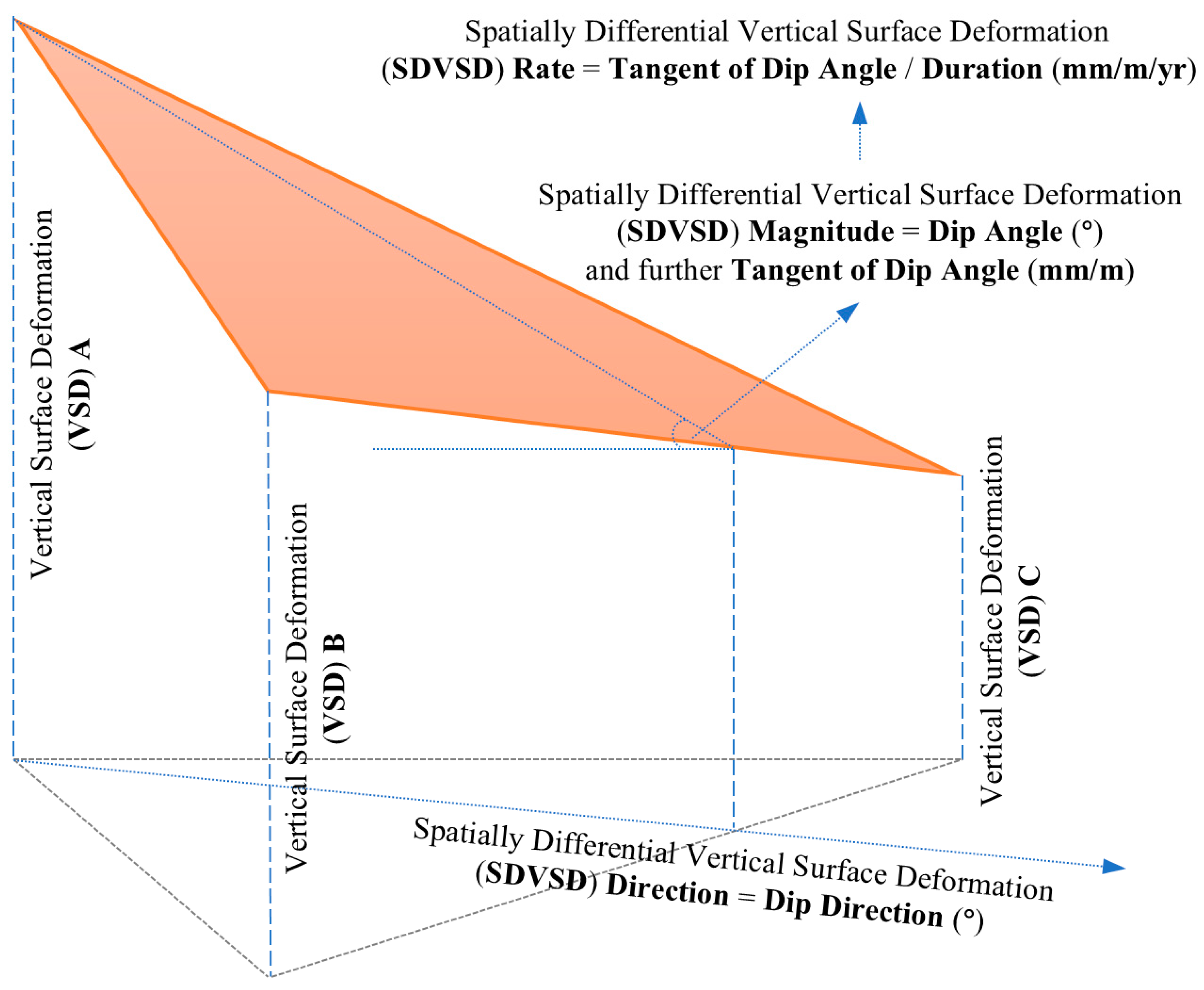
2.1. Principles of SDVSD Quantification

Spatially differential vertical surface deformation (SDVSD) refers to spatially uneven vertical surface deformation (VSD) and thus must be characterized and quantified with respect to a finite spatial unit. For discretely distributed deformation observation locations such as PS points or leveling points, a triangle network is a space tessellation that is ideal for the quantification of SDVSD. Consider a triangle unit formed by three non-collinear observation points. It becomes tilted when different degrees of VSD are observed at the three observation points (Figure 1), which means that the three vertices have different vertical coordinates. Consequently, SDVSD in this triangle unit can be characterized based on its inclination. Specifically, the direction and magnitude of SDVSD can be quantified by the dip direction and dip angle of the tilted triangle unit, respectively (Figure 1). For better clarity, the SDVSD magnitude can be further expressed as the tangent of the dip angle, which implies the amount of VSD difference occurring per unit distance along the dip direction. Accordingly, the SDVSD rate value can be expressed as the dip angle tangent divided by the observation duration (Figure 1), which implies the amount of VSD difference occurring per unit distance along the dip direction per unit duration. It is important to note that the SDVSD rate is always positive and does not have a sign. While SDVSD has a direction and a magnitude (rate), VSD has both a sign and a magnitude (rate). The sign of VSD can be considered analogous to its direction, which has only two values: negative (downward) for subsidence and positive (upward) for uplift. Any spatial difference in VSD within the spatial domain will induce SDVSD, whether it arises from differences in negative VSD, positive VSD, or a combination of negative and positive VSD.
Spatial–temporal VSD data are often represented as a two-dimensional (2D) altitude matrix, with each row recording the altitude time series at a specific observation point and each column recording the altitudes of all observation points on a specific observation date. The altitudes in the first column (on the first date) are always set to 0, so that the altitudes on subsequent dates can directly indicate the cumulative VSD (subsidence or uplift) relative to the first date. In addition, a two-column matrix is required to record the x and y coordinates of the observation points, and a one-row vector is needed to record the observation dates. Without loss of generality, assume that the numbers of observation points and observation dates are denoted as NOP and NDT, respectively. Then, for each observation point, there will be a total of NDT–1 cumulative VSD records and, similarly, NDT–1 incremental VSD records. The cumulative VSD on an observation date is defined as its altitude difference relative to the first observation date, and incremental VSD is defined as its altitude difference relative to the preceding date.
Assume that a triangulated space tessellation based on the NOP discretely distributed deformation observation locations yields a total of NTU triangle units. Each triangle unit should have NDT–1 sets of cumulative SDVSD characteristics, as well as NDT–1 sets of incremental SDVSD characteristics. For a specific cumulative or incremental interval, the direction and magnitude of SDVSD are quantified based on the triangle inclination determined by the VSD within this cumulative or incremental interval at the three observation points defining the triangle unit. The rate of SDVSD is then calculated by dividing its magnitude by the date interval. In addition to the SDVSD direction and SDVSD rate, an average VSD rate can also be determined for each triangle unit by dividing the mean VSD of its three vertices (observation points) by the date interval. Thus, for a cumulative or incremental interval, each triangle unit is characterized by three quantities: the SDVSD direction (°), SDVSD rate (mm/m/yr), and VSD rate (mm/yr). Consequently, for the SDVSD direction, SDVSD rate, and VSD rate, a 2 × NTU × (NDT − 1) three-dimensional (3D) quantity matrix is derived. The first dimension (2) indicates that VSD and SDVSD can be expressed in either cumulative or incremental terms.
For each triangle unit, the weighted mean of the incremental characterization quantities over the entire observation period can also be calculated. For instance, for a triangle unit, the weighted mean incremental SDVSD direction is obtained by averaging its SDVSD directions across all incremental intervals, weighted by the corresponding interval lengths. Similarly, the weighted mean incremental SDVSD rate and incremental VSD rate can also be computed by applying the same weighting approach. It is essential to highlight two considerations when performing statistical analysis on the SDVSD direction, whether in the temporal or spatial domain. First, circular statistics must be employed for SDVSD direction statistics. Second, NaN values for the SDVSD direction may occur in certain triangle units and intervals when there is no spatial variation in VSD; these values should be ignored during statistical analysis.

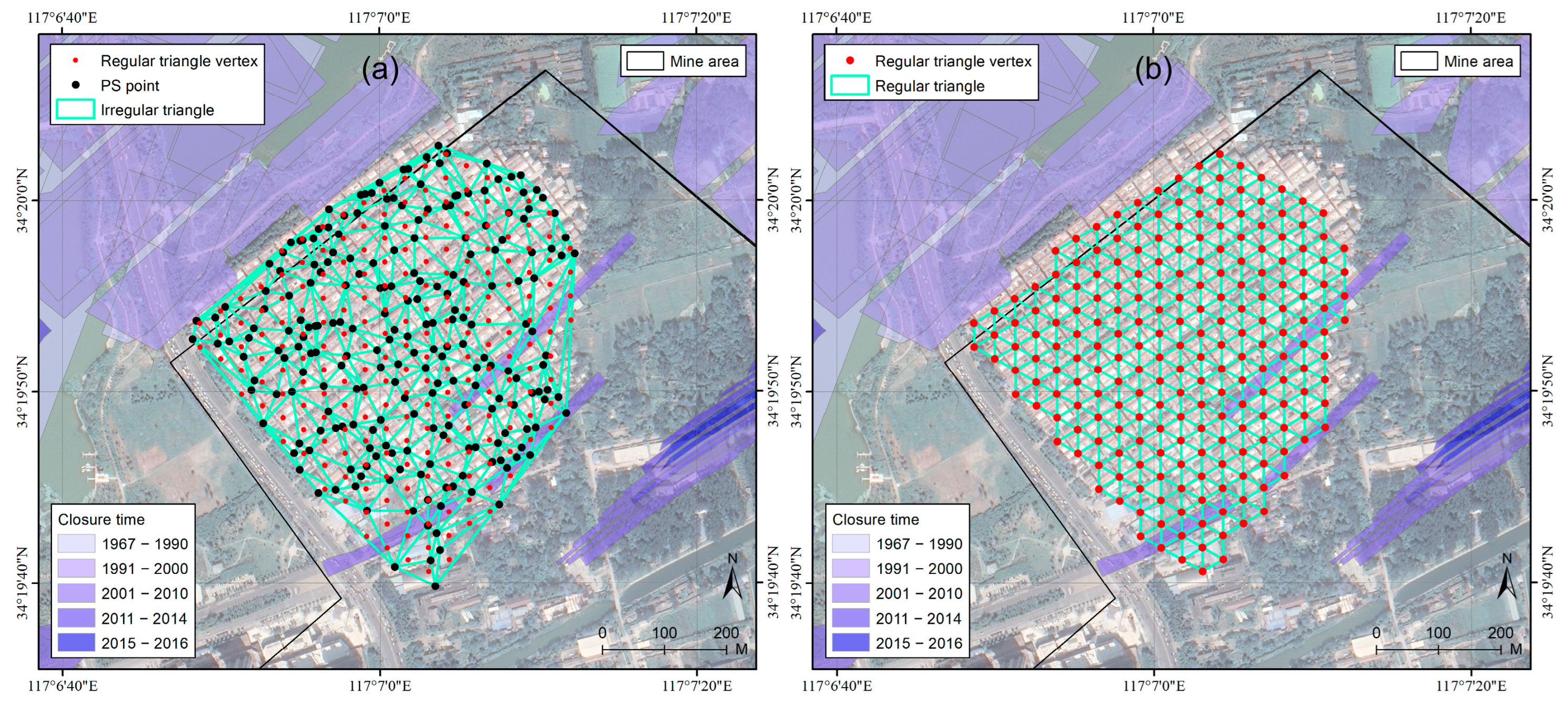
2.2. Construction of Regular Triangle Network

For unevenly distributed PS deformation observation points, although it is straightforward to tessellate space with an irregular triangle network (ITN) using Delaunay triangulation, a regularly tessellated space is preferable to irregular triangulation due to the uniformity of characterization units. Discrepancies in the size and shape of irregular triangles introduce uncertainties when comparing SDVSD quantities among triangle units. A more robust approach is to characterize SDVSD based on a regular triangle network (RTN). Therefore, an RTN is constructed to tessellate the space into uniformly sized triangle units, with nodes interpolated from PSI-derived VSD data. Nevertheless, constructing an ITN is a prerequisite for the construction of an RTN.
The construction of an RTN requires the definition of three key aspects, i.e., the size, orientation, and centroid locations of the regular (equilateral) triangle units. The orientation of all regular triangle units is uniform and corresponds to the extension direction of their central axes. Once the size and orientation are determined, defining the centroids of all regular triangle units requires only the definition of a single reference centroid. The necessity of constructing an ITN first arises from the need to determine these parameters. The average size of all irregular triangle units generated from PS points serves as an appropriate reference for the size of regular triangle units. Similarly, the weighted mean inclination direction of all irregular triangle units can be used as the orientation of regular triangles, ensuring that the adopted orientation reflects the overall directional tendency of all irregular triangle units. Specifically, according to the principles of SDVSD quantification, each irregular triangle unit already has a weighted mean incremental SDVSD direction over the entire observation period. Then, an average orientation for all irregular triangle units can be derived by weighting these values according to the triangle sizes. In other words, the weighted averaging of the SDVSD direction is first performed in the temporal domain for each irregular triangle unit and subsequently in the spatial domain for all irregular triangle units. In addition, the centroid of the convex hull of all PS points is adopted as the reference centroid for a regular triangle unit, ensuring unbiased coverage and preventing marginal PS points from being underrepresented in the RTN.
Once the size, orientation, and centroid are established, the vertices of the regular triangle units covering the entire study area can be generated. For each regular triangle vertex, its altitude and corresponding VSD values are interpolated from the enclosing (tilted) irregular triangle unit, with respect to each observation date and interval. The need to define VSD values for regular triangle vertices constitutes the second reason for initially constructing the ITN. Let NRV and NRT represent the number of regular triangle vertices and regular triangle units, respectively. Then, a NRV × NDT 2D altitude matrix can be constructed for all regular triangle vertices across the observation dates. Using this altitude matrix and following the SDVSD quantification principles, a 2 × NRT × (NDT − 1) 3D quantity matrix can be derived, representing the SDVSD direction (°), SDVSD rate (mm/m/yr), and VSD rate (mm/yr). The first dimension (2) indicates that both VSD and SDVSD can be expressed in either cumulative or incremental terms. Finally, for each regular triangle unit, the weighted mean values of the incremental SDVSD direction, incremental SDVSD rate, and incremental VSD rate over the entire observation period can be calculated.

3. Study Area and Data
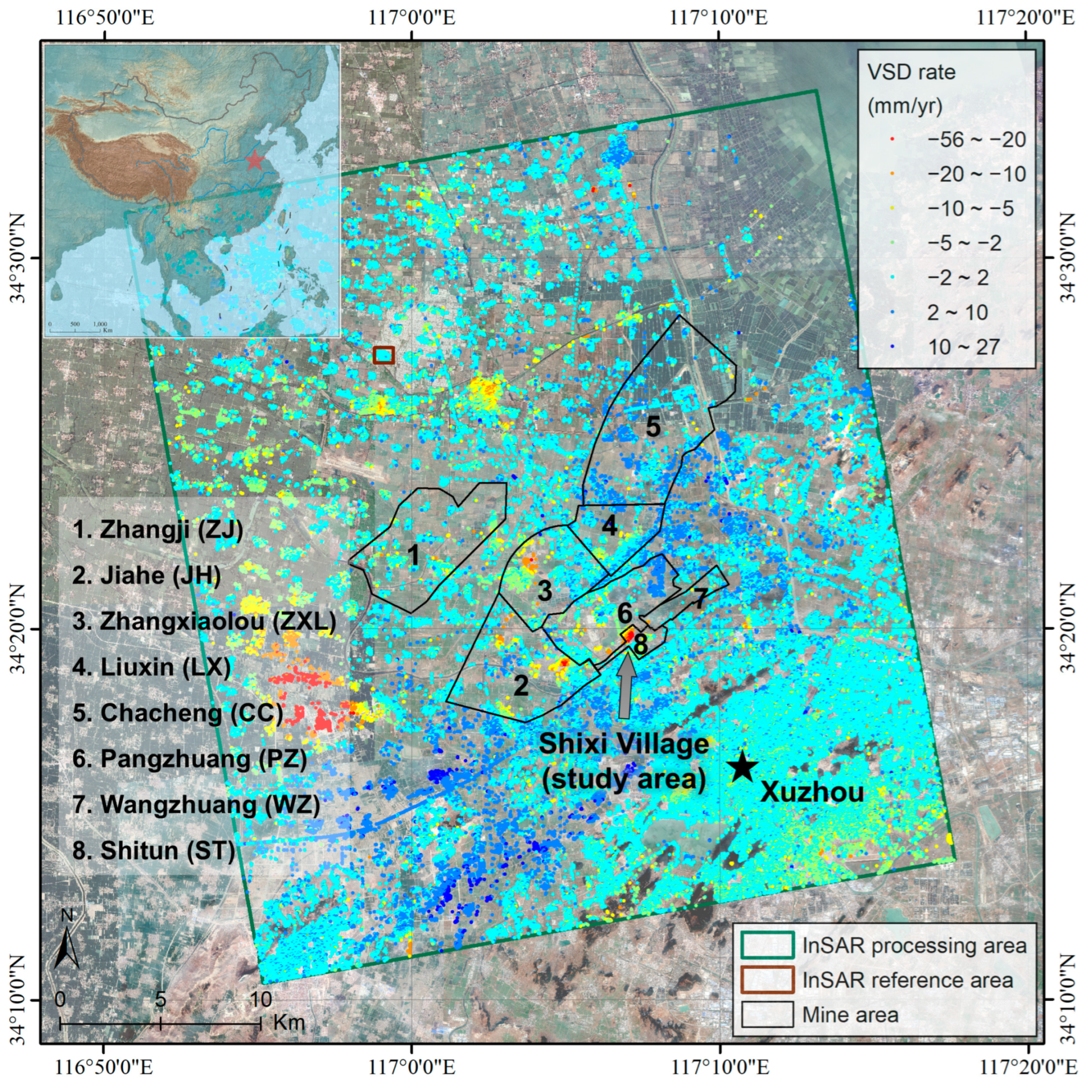
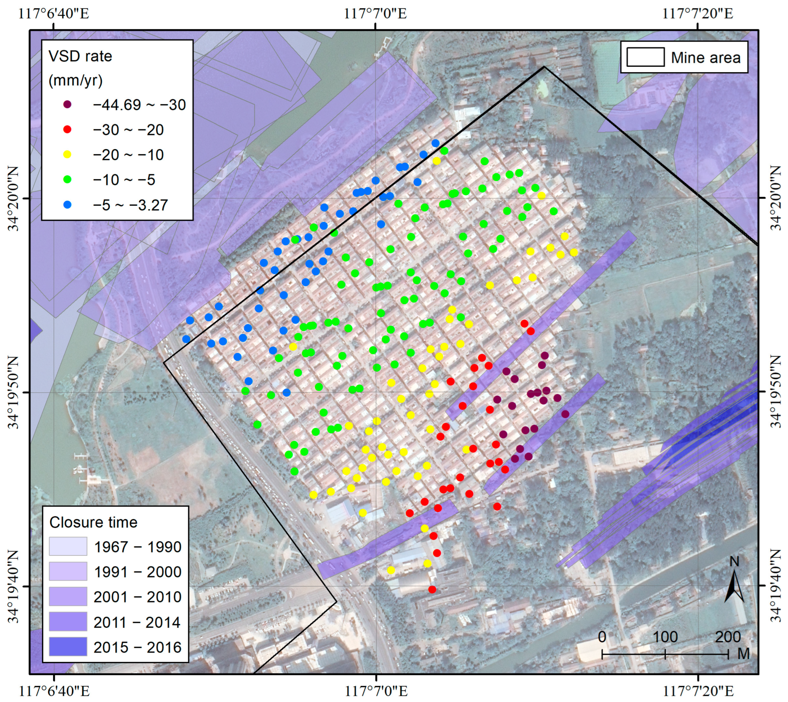
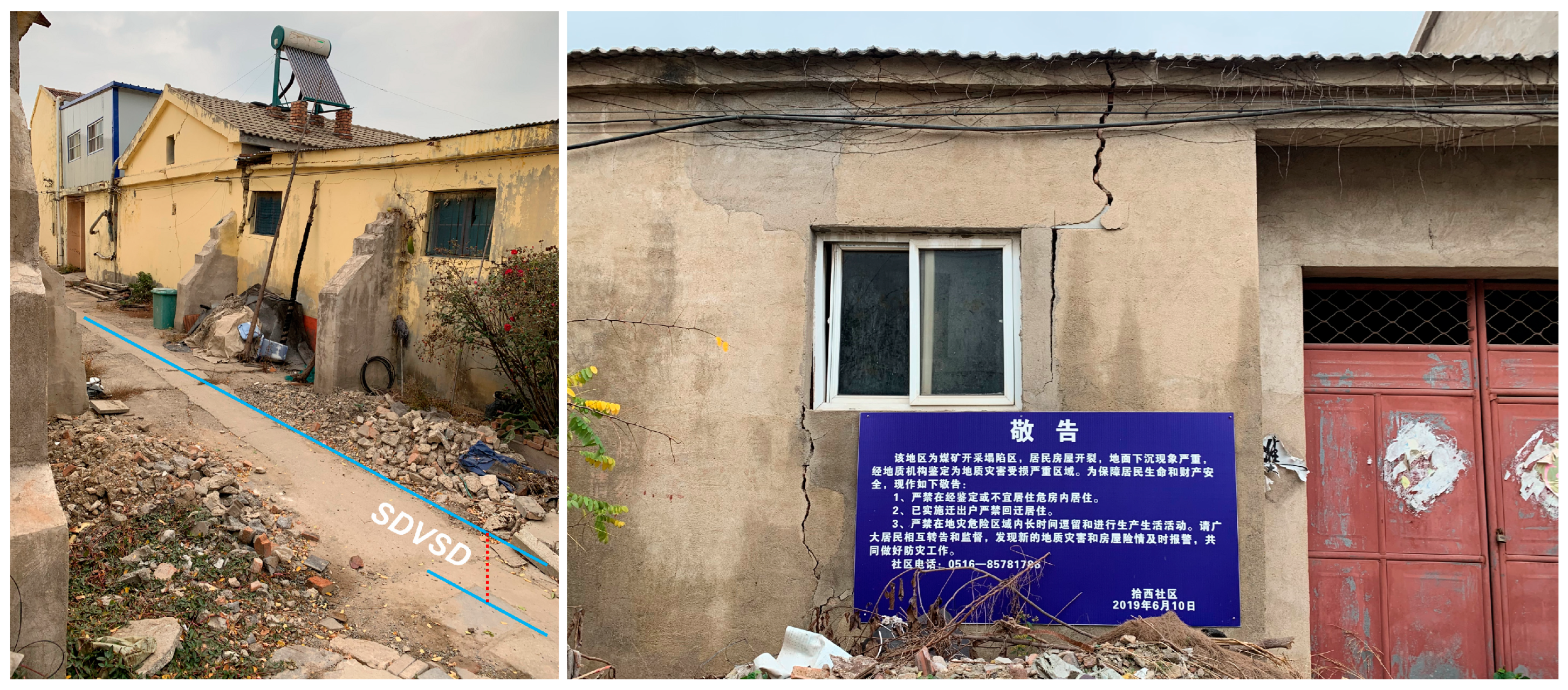
3.1. Study Area

The city of Xuzhou (Figure 2), situated in Jiangsu Province, China, experiences a warm temperate climate. The region’s average annual precipitation exceeds 800 mm, and the daily temperatures fluctuate around 14 °C. Xuzhou is located on the alluvial plain of the Yellow River, where the sediment layers can reach over 50 m in thickness. The terrain is largely flat, with an average elevation of approximately 37 m. The region is intersected by numerous river channels. Notably, a historical channel of the Yellow River traverses the area north of the city, running from northwest to southeast and contributing to a slightly elevated landscape compared to its surroundings.
Coal mining in Xuzhou dates back to the late-19th-century Qing dynasty. There are eight primary mines in the coalfield, situated in the northwestern suburbs of Xuzhou (Figure 1): Zhangji (ZJ), Jiahe (JH), Zhangxiaolou (ZXL), Liuxin (LX), Chacheng (CC), Pangzhuang (PZ), Wangzhuang (WZ), and Shitun (ST). The coal strata dip to the northwest, with the depths increasing from under 100 m in the southeast to more than 1000 m in the northwest. The coal measures in this area comprise Upper Carboniferous and Lower Permian formations, with a cumulative thickness approaching 500 m [71]. Around 5–7 seams, totaling 9 m in thickness, are suitable for mining, representing roughly 1.8% of the strata thickness. Longwall mining dominates in these mines, utilizing large, contiguous extraction panels—up to 400 m wide and 4 km long. This method often leads to the subsidence of the overlying rock layers due to the removal of substantial coal volumes. The coalfield in the northwestern suburbs of Xuzhou has experienced substantial subsidence due to mining (Figure 2), as evidenced by the widespread distribution of water bodies in subsidence depressions [72].
The Shitun (ST) mine, which is the closest to Xuzhou’s urban area among the eight mines, was the last to shut down, ceasing operations in January 2017. Shixi Village, located within the Shitun mine and identified as the most significant subsidence center from 2015 to 2020 (Figure 2 and Figure 3) [71], has been selected as the study area to evaluate the proposed RTN-based formal quantification framework for PSI-derived SDVSD. The area of Shixi Village is about 0.27 km2. Notably, the alignment of buildings in Shixi Village (Figure 3) mirrors the northeast-striking direction of the coal strata and the working faces.

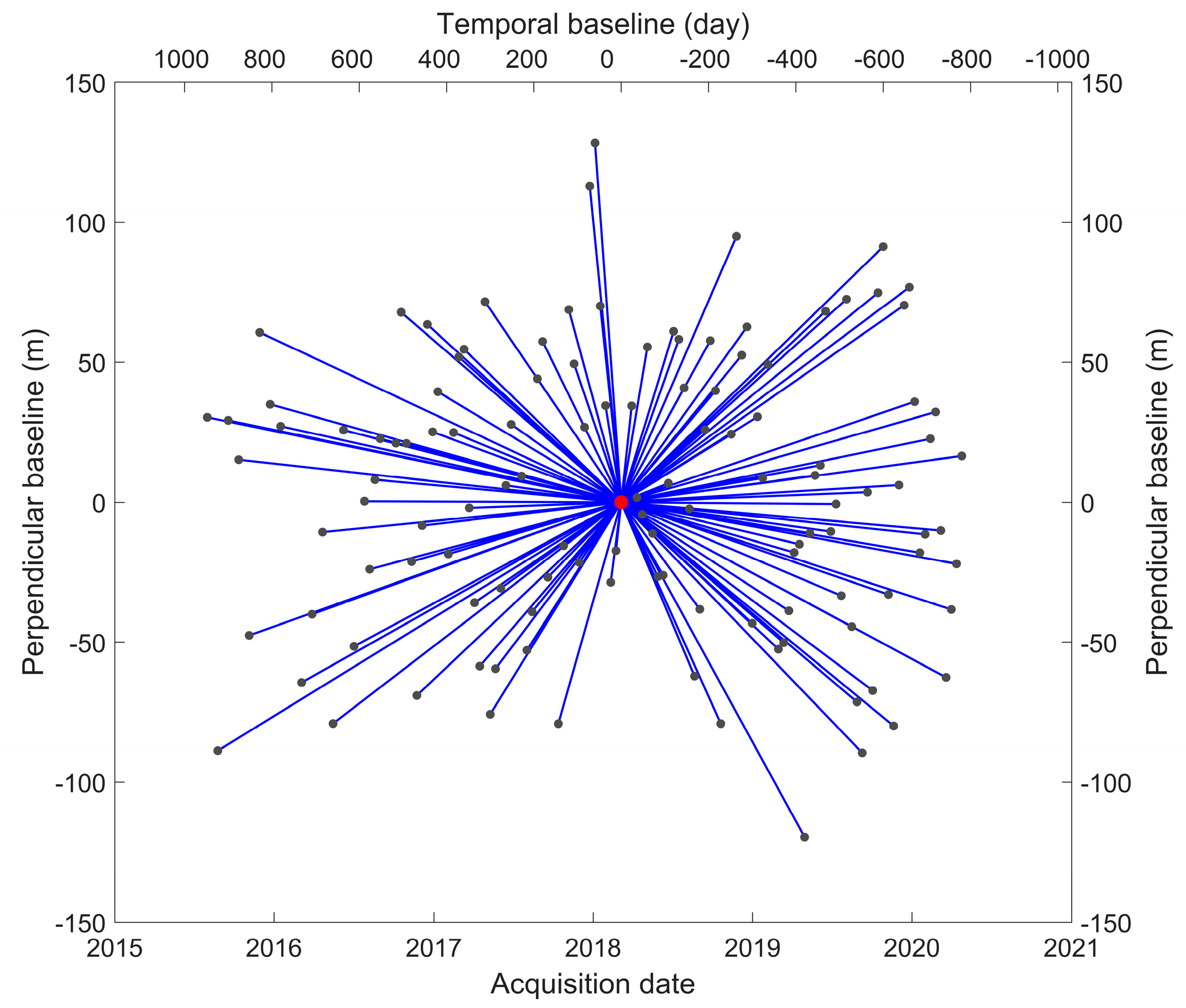
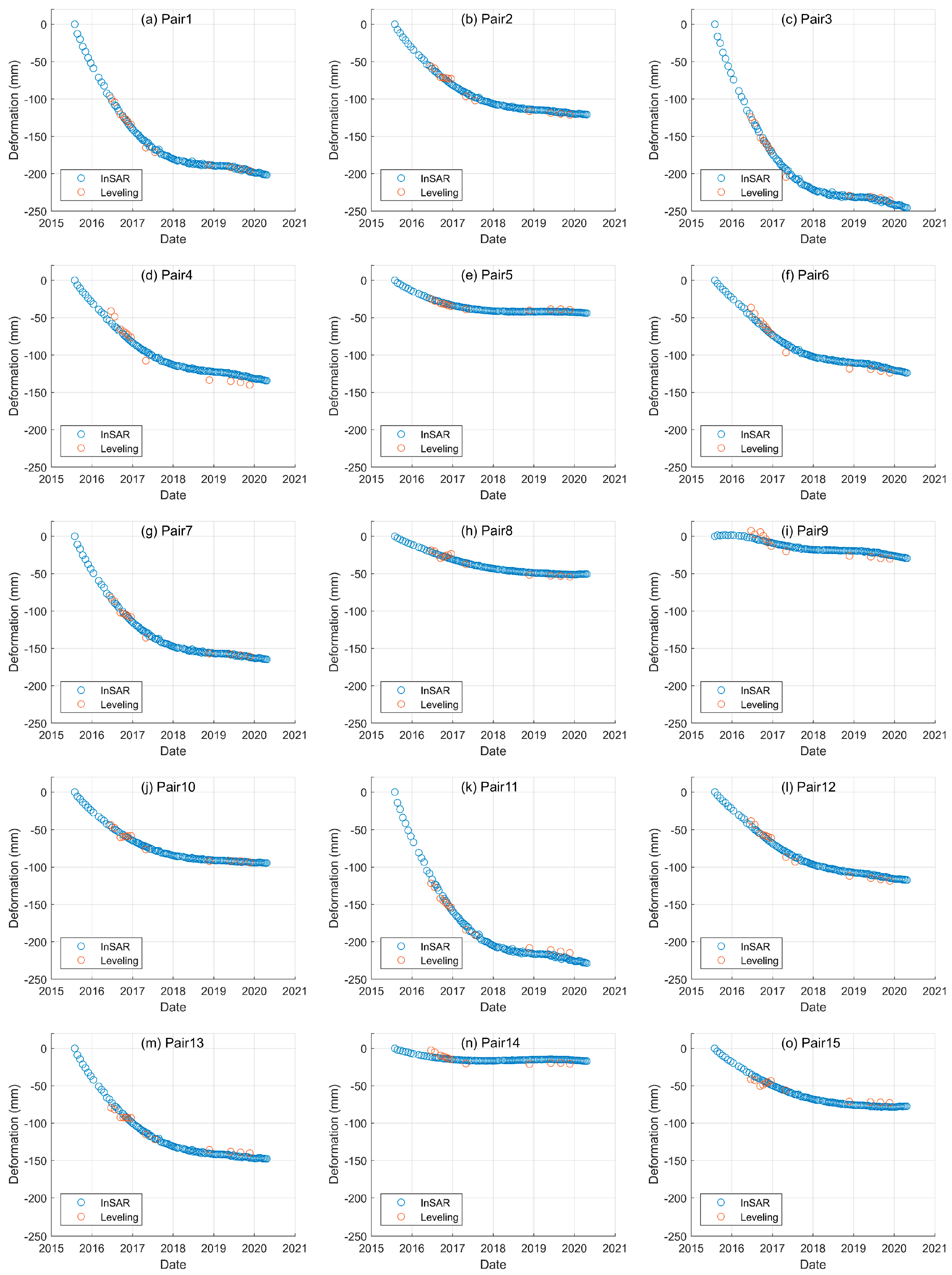
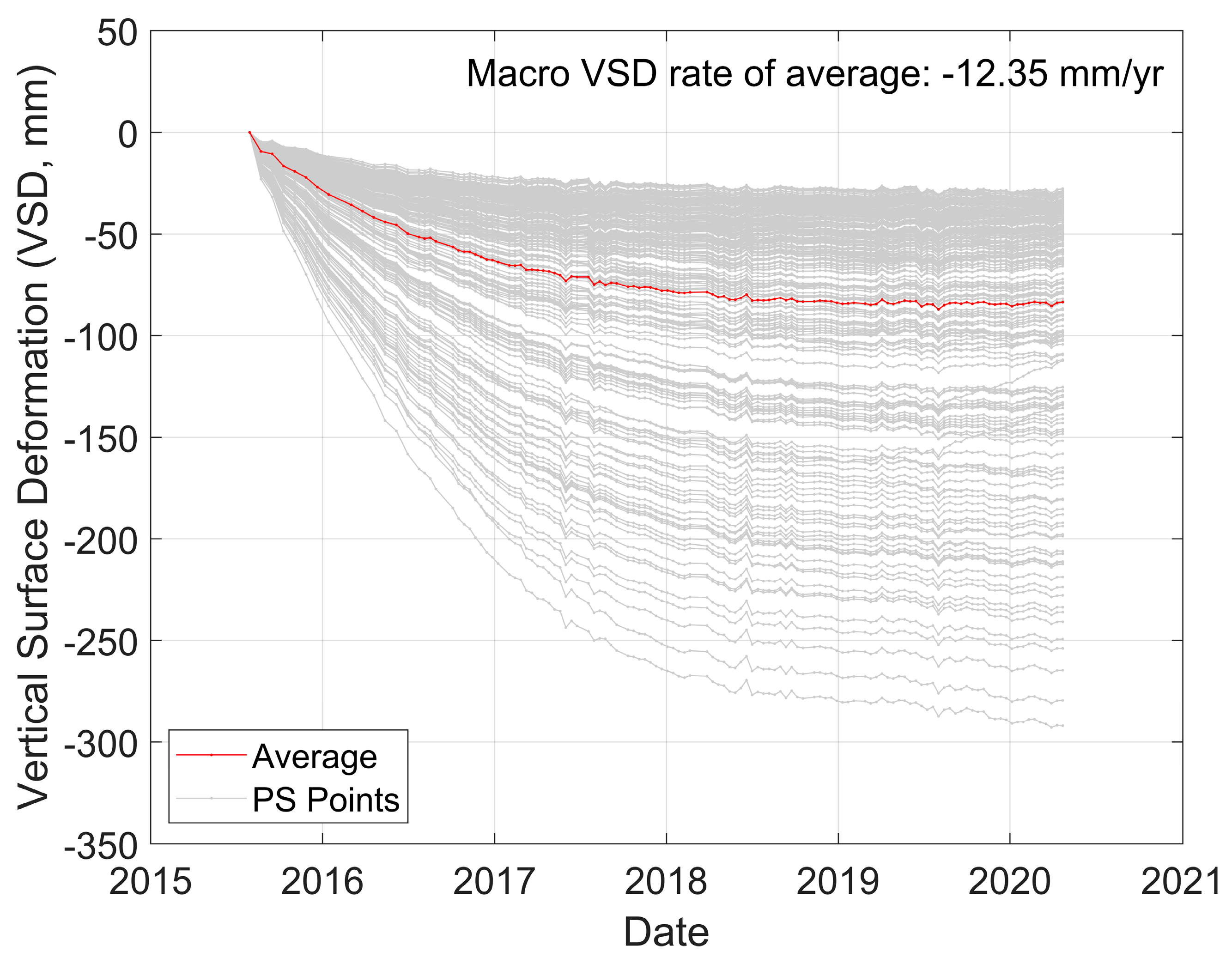
3.2. PSI-Derived VSD Data

Time series InSAR has been widely applied for the study of coalfield-related surface deformations [73,74,75,76,77,78,79,80]. With its capability to provide detailed spatial and temporal deformation data, time series InSAR is ideally suited for investigating the intricate deformation characteristics in the Northwestern Xuzhou coal-mining region. Previous studies have applied time series InSAR to monitor surface deformation in the northwestern suburbs of Xuzhou [71,81,82,83], including deformation history analysis based on the classification of surface deformation time series [71]. However, earlier research has not fully addressed the SDVSD of this region.
The authors had retrieved the VSD of the study area between 30 July 2015 and 22 April 2020 using the PSI technique (Figure 2 and Figure 3) [71]. Small baseline methods were not used because the traditional PS method had already obtained a sufficient number of stable pixels for time series deformation analysis in the study area. Details of the PSI processing can be found in the authors’ previous paper [71]. Necessary details can also be found in the Appendix A. The main text will only provide a brief description.
InSAR time series analysis was conducted using the StaMPS software [40,84,85], a major tool in persistent scatterer interferometry (PSI). A total of 121 Sentinel-1 SAR images (12.66 m projected pixel spacing) were used, spanning 30 July 2015–22 April 2020, with a mostly 12-day revisit time. All images were subset to the InSAR processing area, and all deformations were aligned to a stable reference area away from coal mines (Figure 2). Line-of-sight (LOS) surface deformations were converted to vertical movements under the assumption of vertical displacement only [86]. Singular value decomposition (SVD) was used to filter temporal components of the deformation matrix (114,477 PS points over 120 epochs) to reduce noise [82,87,88]. SVD decomposed this matrix into principal components (PCs), ranked by their variance contributions. Low-order PCs explained most of the variation, capturing primary surface deformation patterns, while high-order PCs represented noise or irrelevant signals and were excluded. Only the first 10 PCs were retained, collectively explaining 76.6% of the variance, with polynomial filtering applied for further noise reduction [82].
The 93 leveling points near PS points (≤25.33 m) in Shixi Village were selected for the optimization and validation of the PSI result [71]. Eight points with the most complete records were used for result optimization. StaMPS parameters that minimized discrepancies between the PSI and leveling data were selected. Specifically, the relative VSD between pairs of leveling points and pairs of PS points that were sufficiently separated was analyzed. Validation involved 85 leveling points with fewer records, generating 2405 eligible point pairs. A similar comparative analysis yielded an average RMSE of 2.45 mm, confirming the reliability of the PSI results. Both optimization and validation confirmed the strong agreement between the PSI and leveling data, ensuring robustness and accuracy.
The macro VSD rates of the 114,477 PS points in the InSAR processing area are shown in Figure 2. In the Shixi study area, a total of 220 PS points were identified, indicating a density of about 815 PS/km2; their macro VSD rates and histories are shown in Figure 3 and Figure 4, respectively. Some PS points, especially those with smaller VSD, exhibited both subsidence and uplift during the SAR data spanning period (Figure 4). Mining activities in Shixi ceased in early 2017. Following mine closures, observations have shown a reduction in subsidence and even surface uplift in some areas [71,81,82,83]. This research focuses on the quantitative characterization of SDVSD in Shixi based on these PSI-derived VSD data.

4. Results

4.1. Regular Triangle Network

The irregular triangle network (ITN) generated by Delaunay triangulation based on the PS points in Shixi is shown in Figure 5a. According to this ITN and the SDVSD characteristics of these irregular triangle units, the edge length, orientation direction, and reference centroid of the regular triangle units were obtained, which were 38.39 m, 120.49°, and (510,784.72 m, 3,800,399.77 m) in the CGCS2000_3_Degree_GK_CM_117E coordinate system, respectively. The generated regular triangle vertices and regular triangle network (RTN) are shown in Figure 5. The total number of regular triangle vertices is 213, close to that of the PS points, resulting in a density of about 789 vertices/km2. The total number of regular triangle units is 371, resulting in a density of about 1374 triangles/km2. The orientation direction of the regular triangle units (120.49°) matches well with the northwest–southeast dip direction of the coal strata in the study area, suggesting that the Shixi study area as a whole underwent southeast-dipping SDVSD during the observation period (Figure 5b). With this RTN, the following section will present the quantitative SDVSD characteristics of the Shixi study area during the observation period (30 July 2015~22 April 2020).

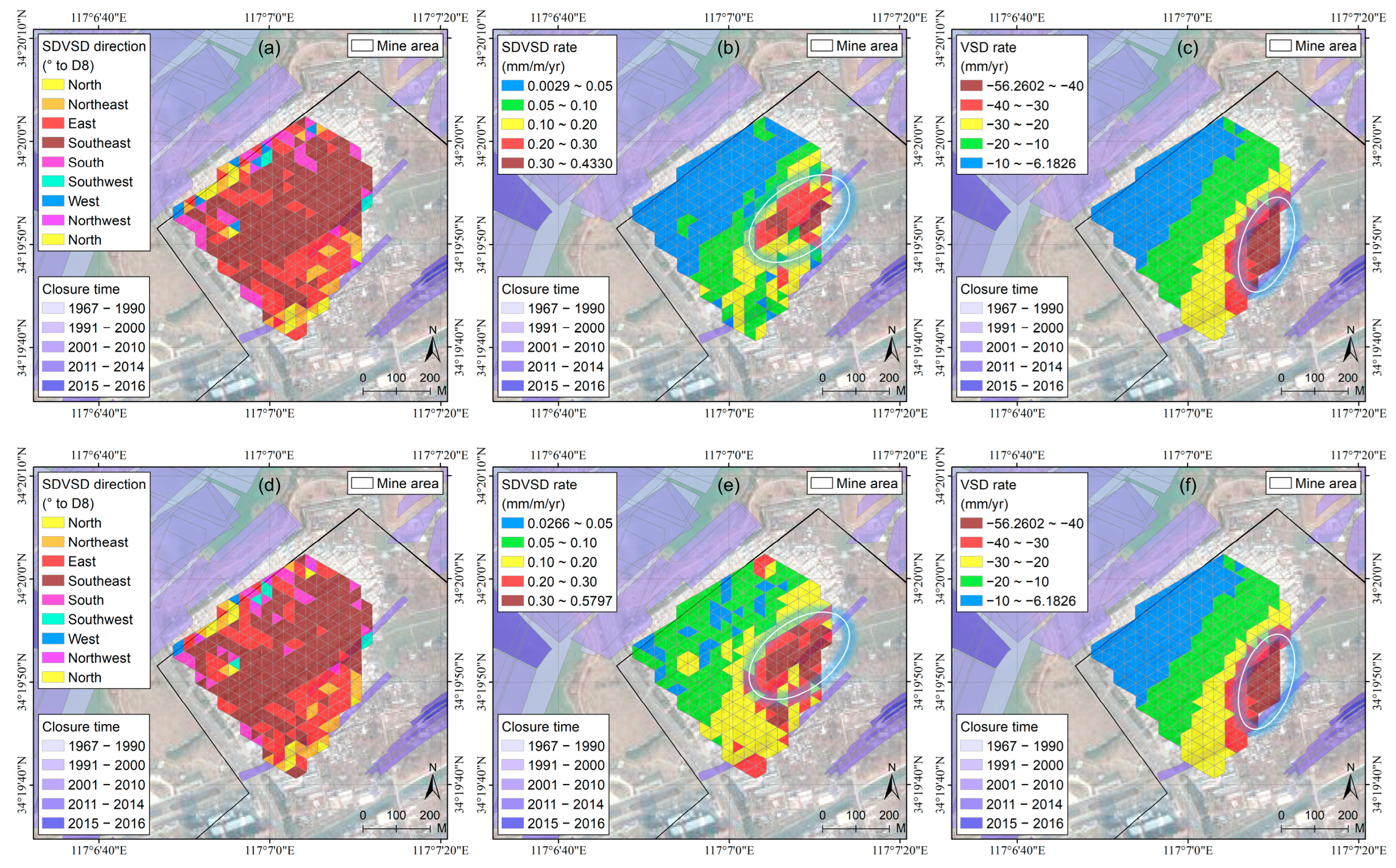
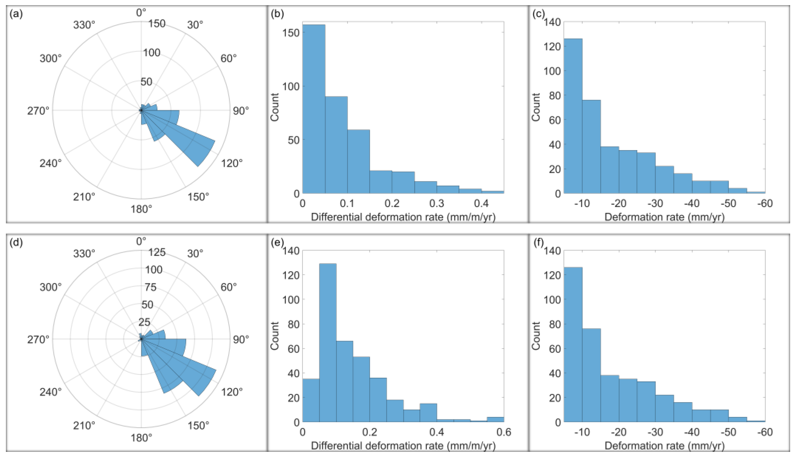
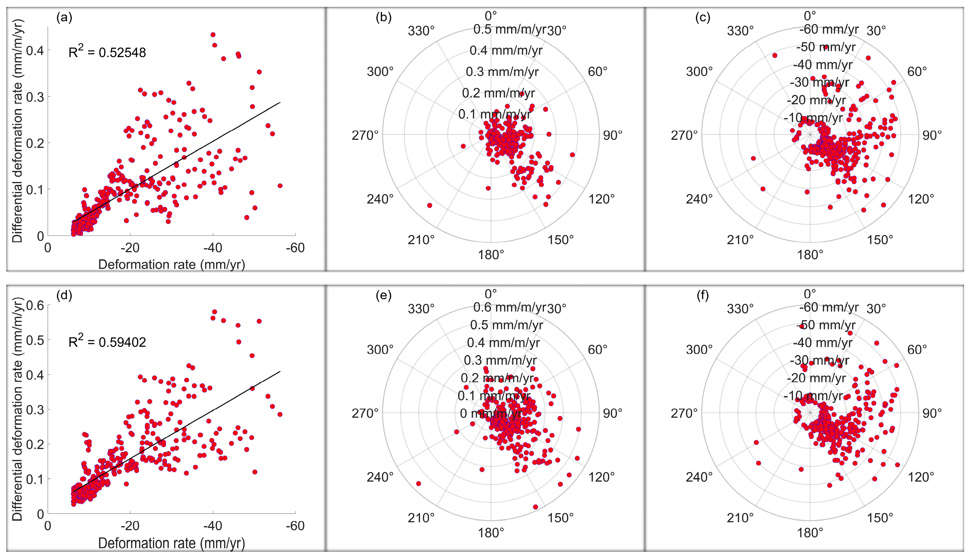
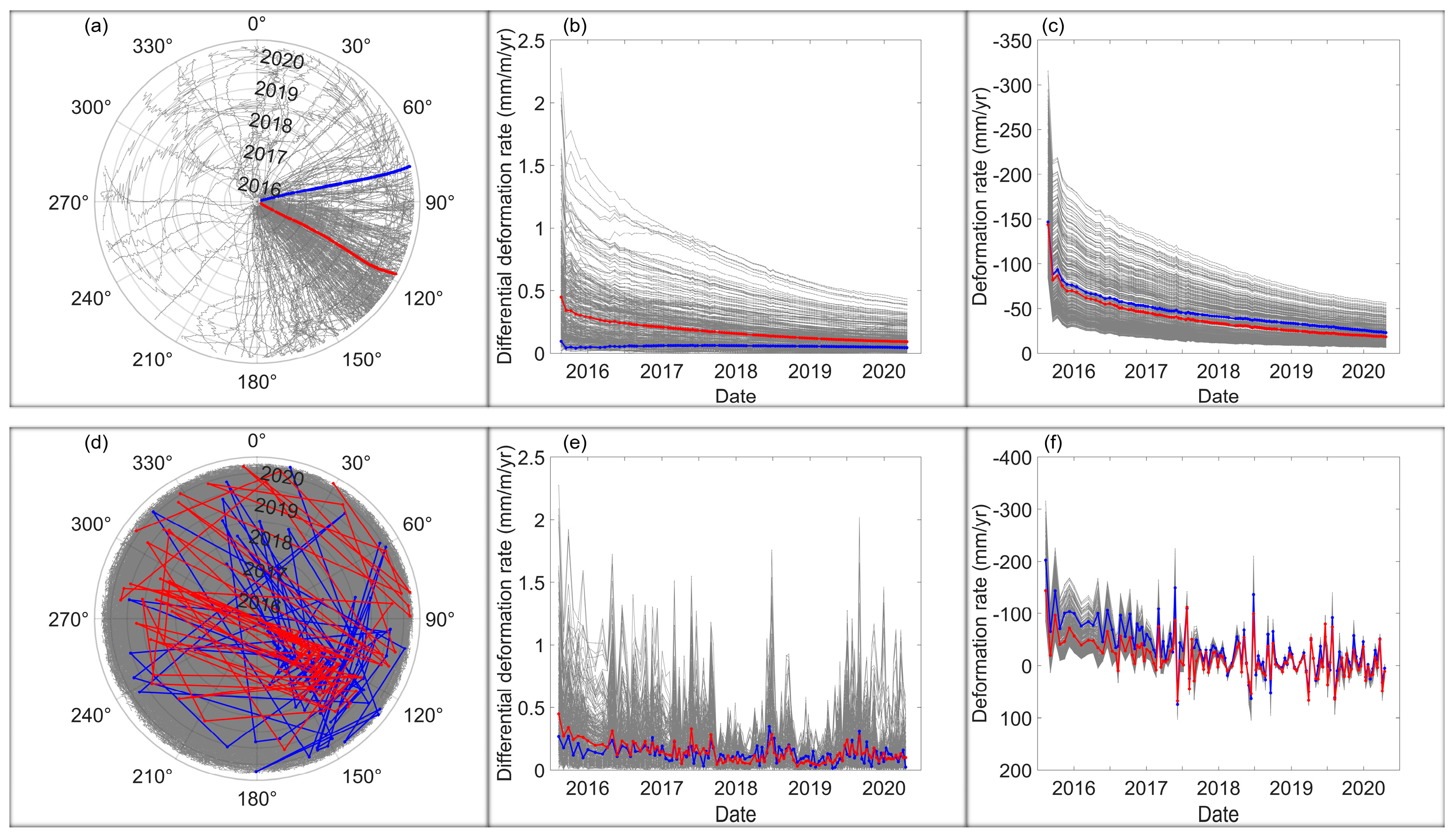
4.2. SDVSD Characteristics

The spatial distribution of the SDVSD and VSD quantities in the Shixi study area during the observation period (30 July 2015~22 April 2020) is shown using the RTN in Figure 6. The statistical characteristics of the SDVSD and VSD quantities among the regular triangle units are shown in Figure 7 and Table 1, using histograms and statistical parameters, respectively. Cumulative quantities represent the values as of the last observation date (i.e., 22 April 2020). Incremental quantities are the mean values of all incremental intervals weighted by the interval length. We can see that the cumulative and incremental SDVSD quantities have a similar spatial distribution pattern (Figure 6) and statistical characteristics (Figure 7; Table 1), while the cumulative VSD rate and the incremental VSD rate are identical (Figure 6 and Figure 7; Table 1). This is because VSD has an additivity property, whereas SDVSD does not. This non-additivity in the temporal domain is a unique property of SDVSD, distinct from that of VSD, suggesting the necessity of paying spatial attention to SDVSD.
Most regular triangle units in the Shixi study area were subjected to southeast-dipping SDVSD during the observation period (Figure 6a,d and Figure 7a,d), with a mean SDVSD direction close to 120° (Table 1), which corresponds to a general southeastward increasing pattern of VSD (Figure 6c,f). The high SDVSD rates, i.e., the high spatial gradients of the VSD rate in Shixi Village, are thought to be related to the locations of the working faces. In the northwest of Shixi Village, there are no working faces, corresponding to low VSD rates, while, in the southeast of Shixi Village, there are working faces with later closure times (Figure 6), resulting in high VSD rates. The uneven distribution of the working faces is thus considered a major cause of the high spatial gradients of VSD (i.e., severe SDVSD). In particular, high SDVSD rates are concentrated around an isolated working face in the southeast of Shixi Village (Figure 6). Severe building damage was also found in the southeast of Shixi Village (Figure 8).
The SDVSD rate and VSD rate are generally correlated, and high values of both the SDVSD rates and VSD rates occur in regular triangle units dipping towards the southeast or east (Figure 9). Nevertheless, they are not necessarily mutually determined. A region with high VSD rates is not necessarily characterized by significant SDVSD. The results of the Shixi case study suggest that the most significant SDVSD does not occur in areas with the highest VSD rates (Figure 6) but, by definition, in areas with the highest spatial gradient of VSD. This difference between SDVSD and VSD again suggests the necessity of paying particular attention to SDVSD.
The temporal evolution of the SDVSD and VSD quantities of the Shixi study area during the observation period (30 July 2015~22 April 2020) is shown in Figure 10. On average, the cumulative SDVSD direction in the Shixi study area remains quite steady during the observation period, keeping close to 120° until around the middle of 2019 and then turning slightly towards the east; meanwhile, both the cumulative SDVSD rate and cumulative VSD rate show an obvious decreasing trend (Figure 10). For most regular triangle units, the standard deviation of the cumulative SDVSD direction time series is quite low, with a mean value of 5.8147° (Figure 11a), suggesting steady temporal evolution. In contrast, the temporal evolution of the incremental SDVSD and VSD quantities fluctuates significantly (Figure 10), which is reflected by high values of the standard deviation and coefficient of variation (Figure 11). SDVSD is not defined solely by a single quantitative value but also exhibits a directional component. The results of the Shixi case study suggest that no obvious pattern can be detected in the temporal evolution of the incremental SDVSD direction (Figure 10d). Nevertheless, the temporal evolution of the incremental SDVSD rate appears to have a seasonal pattern (Figure 10e), similar to that of the incremental VSD rate (Figure 10f). This suggests that seasonal factors such as the temperature and rainfall may impose constraints on SDVSD.

5. Conclusions

The proposed regular triangle network (RTN)-based framework addresses critical limitations in quantifying spatially differential vertical surface deformation (SDVSD) by standardizing spatial units and integrating directional analysis. Traditional methods often struggle with irregular PS point distributions and overlook the directional heterogeneity of deformation spatial gradients. By tessellating the study area into uniform triangular units and interpolating PSI-derived vertical surface deformation (VSD) data, the RTN enables the consistent evaluation of SDVSD in terms of the direction, magnitude, and rate. Key technical innovations include the application of circular statistics to handle directional data and the separation of cumulative and incremental deformation metrics, which reveal the non-additive temporal behaviors unique to SDVSD. This approach not only mitigates spatial biases but also provides a scalable solution for regions with uneven PS points.
The application of the RTN-based framework to the Shixi mining area yielded critical insights into the SDVSD dynamics. Spatially, the predominant southeastward deformation direction (~120°) closely aligns with the dip of the coal strata and the orientation of the mining working faces, underscoring the role of geological and anthropogenic factors in shaping deformation patterns. High SDVSD rates clustered near working faces, correlating with severe building damage. Temporally, seasonal fluctuations in the incremental SDVSD rates further indicated environmental influences. Notably, areas with high VSD rates did not always exhibit significant SDVSD, emphasizing the need for independent spatial gradient analysis. These findings validate the RTN’s utility in linking surface deformation to subsurface conditions and provide actionable data for deformation hazard analysis.
Some limitations still exist, guiding future research. First, while this study formalizes SDVSD quantification and validates it via a case analysis, the driving mechanisms remain unexplored. Factors such as geological structures, groundwater dynamics, and mining parameters likely interact to shape SDVSD patterns, yet their relative contributions are not yet fully understood. Future work should integrate multiple datasets to build coupled models that elucidate causal relationships. In addition, the current framework focuses solely on vertical surface deformation (VSD), whereas real-world deformation involves three-dimensional volumetric changes. Formalizing extended versions of the framework to incorporate full 3D deformation vectors—and further integrating temporal evolution—would enable a four-dimensional (4D) analysis of differential deformation. This generalization requires advanced data fusion techniques and computational methods to handle the increased complexity.

Author Contributions

Conceptualization, L.L. and C.Z.; methodology, L.L. and G.Z.; software, L.L.; validation, C.Z. and L.L.; formal analysis, L.L.; investigation, C.Z., L.L., H.Y., G.Z. and W.W.; resources, C.Z., J.H. and Q.F.; data curation, L.L.; writing—original draft preparation, C.Z. and L.L.; writing—review and editing, C.Z., L.L., H.Y., G.Z. and W.W.; visualization, L.L.; project administration, C.Z. and L.L.; funding acquisition, C.Z. and L.L. All authors have read and agreed to the published version of the manuscript.

Funding

This research was funded by the National Natural Science Foundation of China (Grant No. 42177150), the Provincial Financial (Geological Prospecting) Special Fund of Jiangsu Province in 2019 and 2021, and the Key Project of Innovation LREIS (KPI007). This study is a contribution to the Deep-Time Digital Earth (DDE) Big Science Program.

Data Availability Statement

The data presented in this study are available on request from the corresponding author due to non-disclosure agreement.

Acknowledgments

The authors would like to thank ESA for providing the SAR data and the authors of StaMPS and TRAIN for providing the free InSAR processing scripts.

Conflicts of Interest

The authors declare no conflicts of interest.

Appendix A

The appendix provides additional details regarding the PSI processing. A total of 121 C-band ascending Sentinel-1 SAR images, captured between 30 July 2015 and 22 April 2020, with a projected pixel spacing of approximately 12.66 m, were utilized for PSI analysis. The majority of the SAR images had a revisit interval of 12 days. An image acquired on 4 March 2018 was chosen as the master image, with the temporal and perpendicular baselines for the master–slave image pairs depicted in Figure A1. The maximum temporal baseline extends up to 948 days, while the absolute perpendicular baseline varies between 0.37 m and 128.22 m. To facilitate geocoding and topographic phase removal, ~30-m-resolution Shuttle Radar Topography Mission (SRTM) digital elevation model (DEM) data were employed.
The PSI processing was conducted using the open-source StaMPS software package. To further enhance the deformation results by reducing noise, singular value decomposition (SVD) was applied to decompose and filter the temporal components. SVD is a technique that extracts the principal components (PCs) from the data, enabling the removal of non-essential components (noise) based on the significance of different PCs. The selection of PCs for the construction of the final deformation time series is determined by their contribution and importance. Mathematically, lower-order PCs with minimal contributions are excluded as they have a negligible impact on the deformation time series. Physically, PCs that represent noise or irrelevant signals not pertinent to the study are also discarded. In this study, the first and second PCs account for over 50% of the variation, while the proportions of PC10 and later PCs drop to 1% or less, making their contribution to deformation negligible. As a result, only the first 10 PCs, which collectively explained 76.60% of the variation, were retained to generate the final deformation time series.
Figure A1. Temporal and perpendicular baselines of all 120 master–slave SAR image pairs. The master SAR image, indicated by a red dot, was acquired on 4 March 2018.
Remotesensing 17 01388 g0a1
Leveling data from Shixi Village (Figure A2) were used to optimize and validate the PSI results. Out of 174 leveling points, those with nearby PS points within twice the image pixel spacing (approximately 25.33 m) were chosen, leading to the selection of 93 leveling points for optimization and validation (Figure A2a). Among these, eight leveling points with at least four records from 2018 and 2019 were specifically chosen for optimization (Figure A2b). In other words, of the 93 leveling points with adjacent PS points, these eight leveling points with the most complete measurement history were employed for PSI refinement, while the remaining 85 leveling points were used for validation. It is crucial to recognize that the deformation records of these leveling points are relative to the leveling reference point (Figure A2). If the leveling reference point itself underwent deformation, this would be reflected in the recorded data. Therefore, rigorous PSI optimization and validation should be based on the relative deformation between points. The distinct spatial deformation variations in Shixi Village make it an ideal site for PSI optimization and validation, as well as for the assessment of spatially differential vertical surface deformation (SDVSD).
The optimization of the StaMPS parameters was carried out using the eight leveling points with nearby PS points that had the most comprehensive measurement records (Figure A2b). Specifically, the parameters that minimized discrepancies between the PSI and leveling results were deemed optimal and applied to generate the final PSI deformation results. Due to the absence of adjacent PS points near the leveling reference point in Shixi Village (Figure A2), the comparisons between the PSI and leveling results were based on the relative deformations between points. To ensure a meaningful relative deformation analysis, only 15 pairs of leveling points spaced more than 200 m apart were examined (Figure A2b).
Figure A3 presents the relative deformation histories of the 15 point pairs derived from both PSI and leveling data. The figure demonstrates a strong correlation between the two datasets. The root mean square error (RMSE) between the PSI and leveling deformation time series was employed to quantitatively evaluate the accuracy of the PSI results. Since there were 15 point pairs, this yielded 15 RMSE values. A systematic parameter analysis revealed that the average RMSE for these 15 point pairs reached its minimum when the “unwrap_time_win” parameter in StaMPS was set to 2. This parameter represents the smoothing time window (in days) used to estimate the phase noise distribution for neighboring pixels. The minimum average RMSE was approximately 4.73 mm, which falls below the 5 mm threshold specified by the Ministry of Natural Resources, PRC (DD 2014-11). For this average RMSE, the maximum recorded RMSE was 9.37 mm, while the minimum was 2.17 mm.
Figure A2. Leveling points in Shixi Village utilized for PSI result optimization and validation. The adjacent PS points are depicted as black dots. Panel (a) illustrates all 93 leveling points used for optimization and validation, while panel (b) highlights the 8 leveling points used for optimization. Pairs of points employed to compare the relative deformations between PSI and leveling data are also shown. Numbers in (b) represent the IDs of the leveling and PS points and correspond to table entries indicating point pairs.
Remotesensing 17 01388 g0a2
Following optimization, the validation of the PSI results was performed using 85 leveling points with adjacent PS points but fewer measurement records. The final PSI results, obtained through optimization, were subsequently compared and validated against data from these 85 leveling points. As with the optimization phase, the PSI and leveling results were compared based on the relative deformations between points, and only leveling point pairs spaced more than 200 m apart were analyzed. These 85 leveling points resulted in 2405 eligible point pairs. The average RMSE across these 2405 pairs was calculated to be 2.45 mm, which also meets the 5 mm requirement stipulated in the “DD 2014-11” standard. Since these 85 leveling points had fewer measurement records and shorter observation periods compared to the eight leveling points used for optimization, fewer leveling records were available for PSI comparison, contributing to the lower RMSEs observed during validation.
Figure A3. Relative deformation histories of the 15 point pairs derived from PSI and leveling data during optimization.
Remotesensing 17 01388 g0a3

References

  1. Holzer, T.L.; Pampeyan, E.H. Earth fissures and localized differential subsidence. Water Resour. Res. 1981, 17, 223–227. [Google Scholar] [CrossRef]
  2. Cui, X.; Miao, X.; Yang, S.; Liu, H.; Song, Y.; Liu, H.; Hu, X. Improved prediction of differential subsidence caused by underground mining. Int. J. Rock Mech. Min. Sci. 2000, 37, 615–627. [Google Scholar] [CrossRef]
  3. Shi, M.; Chen, B.; Gong, H.; Li, X.; Chen, W.; Gao, M.; Zhou, C.; Lei, K. Monitoring differential subsidence along the beijing–tianjin intercity railway with multiband SAR data. Int. J. Environ. Res. Public Health 2019, 16, 4453. [Google Scholar] [CrossRef] [PubMed]
  4. Figueroa-Miranda, S.; Hernández-Madrigal, V.M.; Tuxpan-Vargas, J.; Villaseñor-Reyes, C.I. Evolution assessment of structurally-controlled differential subsidence using SBAS and PS interferometry in an emblematic case in Central Mexico. Eng. Geol. 2020, 279, 105860. [Google Scholar] [CrossRef]
  5. de Wit, K.; Lexmond, B.R.; Stouthamer, E.; Neussner, O.; Dörr, N.; Schenk, A.; Minderhoud, P.S. Identifying causes of urban differential subsidence in the Vietnamese Mekong Delta by combining InSAR and field observations. Remote Sens. 2021, 13, 189. [Google Scholar] [CrossRef]
  6. Fernández-Torres, E.A.; Cabral-Cano, E.; Salazar-Tlaczani, L.; Solano-Rojas, D. Economic risk of differential subsidence in Mexico City (2014–2022). Nat. Hazards 2024, 121, 2507–2534. [Google Scholar] [CrossRef]
  7. Rateb, A.; Abotalib, A.Z. Inferencing the land subsidence in the Nile Delta using Sentinel-1 satellites and GPS between 2015 and 2019. Sci. Total Environ. 2020, 729, 138868. [Google Scholar] [CrossRef]
  8. Shirzaei, M.; Freymueller, J.; Tornqvist, T.E.; Galloway, D.L.; Dura, T.; Minderhoud, P.S.J. Measuring, modelling and projecting coastal land subsidence. Nat. Rev. Earth Environ. 2021, 2, 40–58. [Google Scholar] [CrossRef]
  9. Cigna, F.; Tapete, D. Urban growth and land subsidence: Multi-decadal investigation using human settlement data and satellite InSAR in Morelia, Mexico. Sci. Total Environ. 2022, 811, 152211. [Google Scholar] [CrossRef]
  10. Malik, K.; Kumar, D.; Perissin, D.; Pradhan, B. Estimation of ground subsidence of New Delhi, India using PS-InSAR technique and Multi-sensor Radar data. Adv. Space Res. 2022, 69, 1863–1882. [Google Scholar] [CrossRef]
  11. Perissin, D.; Wang, Z.; Lin, H. Shanghai subway tunnels and highways monitoring through Cosmo-SkyMed Persistent Scatterers. ISPRS J. Photogramm. Remote Sens. 2012, 73, 58–67. [Google Scholar] [CrossRef]
  12. Figueroa-Miranda, S.; Tuxpan-Vargas, J.; Ramos-Leal, J.A.; Hernández-Madrigal, V.M.; Villaseñor-Reyes, C.I. Land subsidence by groundwater over-exploitation from aquifers in tectonic valleys of Central Mexico: A review. Eng. Geol. 2018, 246, 91–106. [Google Scholar] [CrossRef]
  13. Scott, C.P.; Arrowsmith, J.R.; Nissen, E.; Lajoie, L.; Maruyama, T.; Chiba, T. The M7 2016 Kumamoto, Japan, Earthquake: 3-D Deformation Along the Fault and Within the Damage Zone Constrained from Differential Lidar Topography. J. Geophys. Res. Solid Earth 2018, 123, 6138–6155. [Google Scholar] [CrossRef]
  14. Schlögl, M.; Widhalm, B.; Avian, M. Comprehensive time-series analysis of bridge deformation using differential satellite radar interferometry based on Sentinel-1. ISPRS J. Photogramm. Remote Sens. 2021, 172, 132–146. [Google Scholar] [CrossRef]
  15. Pawluszek-Filipiak, K.; Borkowski, A. Integration of DInSAR and SBAS Techniques to Determine Mining-Related Deformations Using Sentinel-1 Data: The Case Study of Rydułtowy Mine in Poland. Remote Sens. 2020, 12, 242. [Google Scholar] [CrossRef]
  16. Tao, T.; Han, K.; Yao, X.; Chen, X.; Wu, Z.; Yao, C.; Tian, X.; Zhou, Z.; Ren, K. Identification of Ground Fissure Development in a Semi-Desert Aeolian Sand Area Induced from Coal Mining: Utilizing UAV Images and Deep Learning Techniques. Remote Sens. 2024, 16, 1046. [Google Scholar] [CrossRef]
  17. Castellazzi, P.; Garfias, J.; Martel, R. Assessing the efficiency of mitigation measures to reduce groundwater depletion and related land subsidence in Querétaro (Central Mexico) from decadal InSAR observations. Int. J. Appl. Earth Obs. Geoinf. 2021, 105, 102632. [Google Scholar] [CrossRef]
  18. Ouyang, L.; Zhao, Z.; Zhou, D.; Cao, J.; Qin, J.; Cao, Y.; He, Y. Study on the Relationship between Groundwater and Land Subsidence in Bangladesh Combining GRACE and InSAR. Remote Sens. 2024, 16, 3715. [Google Scholar] [CrossRef]
  19. Wright, T.J.; Parsons, B.E.; Lu, Z. Toward mapping surface deformation in three dimensions using InSAR. Geophys. Res. Lett. 2004, 31, L01607. [Google Scholar] [CrossRef]
  20. Perissin, D.; Wang, T. Time-Series InSAR Applications Over Urban Areas in China. IEEE J. Sel. Top. Appl. Earth Obs. Remote Sens. 2011, 4, 92–100. [Google Scholar] [CrossRef]
  21. Lee, C.W.; Lu, Z.; Jung, H.S. Simulation of time-series surface deformation to validate a multi-interferogram InSAR processing technique. Int. J. Remote Sens. 2012, 33, 7075–7087. [Google Scholar] [CrossRef]
  22. Liao, M.S.; Tang, J.; Wang, T.; Balz, T.; Zhang, L. Landslide monitoring with high-resolution SAR data in the Three Gorges region. Sci. China Earth Sci. 2012, 55, 590–601. [Google Scholar] [CrossRef]
  23. Hu, J.; Li, Z.W.; Ding, X.L.; Zhu, J.J.; Zhang, L.; Sun, Q. Resolving three-dimensional surface displacements from InSAR measurements: A review. Earth-Sci. Rev. 2014, 133, 1–17. [Google Scholar] [CrossRef]
  24. Meng, Y.; Lan, H.; Li, L.; Wu, Y.; Li, Q. Characteristics of surface deformation detected by X-band SAR interferometry over sichuan-tibet grid connection project area, China. Remote Sens. 2015, 7, 12265–12281. [Google Scholar] [CrossRef]
  25. Chen, F.; Guo, H.; Ma, P.; Lin, H.; Wang, C.; Ishwaran, N.; Hang, P. Radar interferometry offers new insights into threats to the Angkor site. Sci. Adv. 2017, 3, e1601284. [Google Scholar] [CrossRef]
  26. Yang, Z.; Li, Z.; Zhu, J.; Yi, H.; Hu, J.; Feng, G. Deriving Dynamic Subsidence of Coal Mining Areas Using InSAR and Logistic Model. Remote Sens. 2017, 9, 125. [Google Scholar] [CrossRef]
  27. Dai, K.; Liu, G.; Li, Z.; Ma, D.; Wang, X.; Zhang, B.; Tang, J.; Li, G. Monitoring highway stability in permafrost regions with X-band temporary scatterers stacking InSAR. Sensors 2018, 18, 1876. [Google Scholar] [CrossRef]
  28. Zhao, C.; Liu, C.; Zhang, Q.; Lu, Z.; Yang, C. Deformation of Linfen-Yuncheng Basin (China) and its mechanisms revealed by Π-RATE InSAR technique. Remote Sens. Environ. 2018, 218, 221–230. [Google Scholar] [CrossRef]
  29. Li, L.; Yao, X.; Yao, J.; Zhou, Z.; Feng, X.; Liu, X. Analysis of deformation characteristics for a reservoir landslide before and after impoundment by multiple D-InSAR observations at Jinshajiang River, China. Nat. Hazards 2019, 98, 719–733. [Google Scholar] [CrossRef]
  30. Wang, B.; Zhao, C.; Zhang, Q.; Peng, M. Sequential InSAR time series deformation monitoring of land subsidence and rebound in Xi’an, China. Remote Sens. 2019, 11, 2854. [Google Scholar] [CrossRef]
  31. Zhang, X.; Zhang, H.; Wang, C.; Tang, Y.; Zhang, B.; Wu, F.; Wang, J.; Zhang, Z. Time-series InSAR monitoring of permafrost freeze-thaw seasonal displacement over Qinghai-Tibetan Plateau using sentinel-1 data. Remote Sens. 2019, 11, 1000. [Google Scholar] [CrossRef]
  32. Zhang, Y.; Liu, Y.; Jin, M.; Jing, Y.; Liu, Y.; Liu, Y.; Sun, W.; Wei, J.; Chen, Y. Monitoring land subsidence in wuhan city (China) using the SBAS-INSAR method with radarsat-2 imagery data. Sensors 2019, 19, 743. [Google Scholar] [CrossRef]
  33. Han, Y.; Zou, J.; Lu, Z.; Qu, F.; Kang, Y.; Li, J. Ground Deformation of Wuhan, China, Revealed by Multi-Temporal InSAR Analysis. Remote Sens. 2020, 12, 3788. [Google Scholar] [CrossRef]
  34. Zhao, X.; Lan, H.; Li, L.; Zhang, Y.; Zhou, C. A Multiple-Regression Model Considering Deformation Information for Atmospheric Phase Screen Compensation in Ground-Based SAR. IEEE Trans. Geosci. Remote Sens. 2020, 58, 777–789. [Google Scholar] [CrossRef]
  35. Zhou, C.; Gong, H.; Chen, B.; Gao, M.; Cao, Q.; Cao, J.; Duan, L.; Zuo, J.; Shi, M. Land subsidence response to dierent land use types and water resource utilization in Beijing-Tianjin-Hebei, China. Remote Sens. 2020, 12, 457. [Google Scholar] [CrossRef]
  36. Zhou, C.; Lan, H.; Gong, H.; Zhang, Y.; Warner, T.A.; Clague, J.J.; Wu, Y. Reduced rate of land subsidence since 2016 in Beijing, China: Evidence from Tomo-PSInSAR using RadarSAT-2 and Sentinel-1 datasets. Int. J. Remote Sens. 2020, 41, 1259–1285. [Google Scholar] [CrossRef]
  37. Dou, J.; Xing, K.; Wang, L.; Guo, H.; Wang, D.; Peng, Y.; Xiang, X.; Ciren, D.; Zhang, S.; Zhang, L.; et al. Air-Space-Ground Synergistic Observations for Rapid Post-Seismic Disaster Assessment of 2025 Ms6.8 Xigazê Earthquake, Xizang. J. Earth Sci. 2025. [Google Scholar] [CrossRef]
  38. Ferretti, A.; Prati, C.; Rocca, F. Permanent scatterers in SAR interferometry. IEEE Trans. Geosci. Remote Sens. 2001, 39, 8–20. [Google Scholar] [CrossRef]
  39. Hilley, G.E.; Bürgmann, R.; Ferretti, A.; Novali, F.; Rocca, F. Dynamics of slow-moving landslides from permanent scatterer analysis. Science 2004, 304, 1952–1955. [Google Scholar] [CrossRef]
  40. Hooper, A.; Segall, P.; Zebker, H. Persistent scatterer interferometric synthetic aperture radar for crustal deformation analysis, with application to Volcán Alcedo, Galápagos. J. Geophys. Res. Solid Earth 2007, 112, B07407. [Google Scholar] [CrossRef]
  41. Sousa, J.J.; Hooper, A.J.; Hanssen, R.F.; Bastos, L.C.; Ruiz, A.M. Persistent Scatterer InSAR: A comparison of methodologies based on a model of temporal deformation vs. spatial correlation selection criteria. Remote Sens. Environ. 2011, 115, 2652–2663. [Google Scholar] [CrossRef]
  42. Lan, H.; Li, L.; Liu, H.; Yang, Z. Complex urban infrastructure deformation monitoring using high resolution PSI. IEEE J. Sel. Top. Appl. Earth Obs. Remote Sens. 2012, 5, 643–651. [Google Scholar] [CrossRef]
  43. Lan, H.; Gao, X.; Liu, H.; Yang, Z.; Li, L. Integration of TerraSAR-X and PALSAR PSI for detecting ground deformation. Int. J. Remote Sens. 2013, 34, 5393–5408. [Google Scholar] [CrossRef]
  44. Crosetto, M.; Monserrat, O.; Cuevas-González, M.; Devanthéry, N.; Crippa, B. Persistent Scatterer Interferometry: A review. ISPRS J. Photogramm. Remote Sens. 2016, 115, 78–89. [Google Scholar] [CrossRef]
  45. Ge, D.; Zhang, L.; Li, M.; Liu, B.; Wang, Y. Beijing subway tunnelings and high-speed railway subsidence monitoring with PSInSAR and TerraSAR-X data. In Proceedings of the 2016 IEEE International Geoscience and Remote Sensing Symposium (IGARSS), Beijing, China, 10–15 July 2016; pp. 6883–6886. [Google Scholar] [CrossRef]
  46. Yang, H.; Peng, J.; Wang, B.; Song, Y.; Zhang, D.; Li, L. Ground deformation monitoring of Zhengzhou city from 2012 to 2013 using an improved IPTA. Nat. Hazards 2016, 80, 1–17. [Google Scholar] [CrossRef]
  47. Wang, C.; Zhang, Z.; Zhang, H.; Wu, Q.; Zhang, B.; Tang, Y. Seasonal deformation features on Qinghai-Tibet railway observed using time-series InSAR technique with high-resolution TerraSAR-X images. Remote Sens. Lett. 2017, 8, 1–10. [Google Scholar] [CrossRef]
  48. Fiaschi, S.; Holohan, E.P.; Sheehy, M.; Floris, M. PS-InSAR analysis of Sentinel-1 data for detecting ground motion in temperate oceanic climate zones: A case study in the Republic of Ireland. Remote Sens. 2019, 11, 348. [Google Scholar] [CrossRef]
  49. Liu, X.; Wang, Y.; Yan, S.; Shao, Y.; Zhou, H.; Li, Y. Ground subsidence characteristics associated with urbanization in East China analyzed with a Sentinel-1A-based InSAR time series approach. Bull. Eng. Geol. Environ. 2019, 78, 4003–4015. [Google Scholar] [CrossRef]
  50. Xue, F.; Lv, X.; Dou, F.; Yun, Y. A Review of Time-Series Interferometric SAR Techniques: A Tutorial for Surface Deformation Analysis. IEEE Geosci. Remote Sens. Mag. 2020, 8, 22–42. [Google Scholar] [CrossRef]
  51. Yang, Y.; Dou, J.; Merghadi, A.; Liang, W.; Dong, A.; Xiong, D.; Zhang, L. Advanced Prediction of Landslide Deformation through Temporal Fusion Transformer and Multivariate Time Series Clustering of InSAR: Insights from the Badui Region, Eastern Tibet. IEEE Trans. Geosci. Remote Sens. 2024, 62, 4514219. [Google Scholar] [CrossRef]
  52. Yang, M.; Wang, R.; Li, M.; Liao, M. A PSI targets characterization approach to interpreting surface displacement signals: A case study of the Shanghai metro tunnels. Remote Sens. Environ. 2022, 280, 113150. [Google Scholar] [CrossRef]
  53. Wang, K.; Chen, J. Accurate persistent scatterer identification based on phase similarity of radar pixels. IEEE Trans. Geosci. Remote Sens. 2022, 60, 5118513. [Google Scholar] [CrossRef]
  54. Wu, H.; Zhang, Y.; Kang, Y.; Wei, J.; Lu, Z.; Yan, W.; Wang, H.; Liu, Z.; Lv, X.; Zhou, M. SAR interferometry on full scatterers: Mapping ground deformation with ultra-high density from space. Remote Sens. Environ. 2024, 302, 113965. [Google Scholar] [CrossRef]
  55. Zhou, D.; Zhao, Z. Optimal algorithm for distributed scatterer InSAR phase estimation based on cross-correlation complex coherence matrix. Int. J. Appl. Earth Obs. Geoinf. 2024, 134, 104214. [Google Scholar] [CrossRef]
  56. Mora, O.; Lanari, R.; Mallorqui, J.J.; Berardino, P.; Sansosti, E. A new algorithm for monitoring localized deformation phenomena based on small baseline differential SAR interferogram. In Proceedings of the IEEE International Geoscience and Remote Sensing Symposium, Toronto, ON, Canada, 24–28 June 2002; pp. 1237–1239. [Google Scholar] [CrossRef]
  57. Wang, S.; Zhang, G.; Chen, Z.; Cui, H.; Zheng, Y.; Xu, Z.; Li, Q. Surface deformation extraction from small baseline subset synthetic aperture radar interferometry (SBAS-InSAR) using coherence-optimized baseline combinations. GISci. Remote Sens. 2022, 59, 295–309. [Google Scholar] [CrossRef]
  58. Yan, M.; Zhao, C.; Liu, X.; Wang, B. Sequential SBAS-InSAR Backward Estimation of Deformation Time Series. IEEE Geosci. Remote Sens. Lett. 2024, 21, 4001505. [Google Scholar] [CrossRef]
  59. Azadnejad, S.; Esmaeili, M.; Maghsoudi, Y.; Donohue, S.; Azar, M.K. Extending polarimetric optimization of multi-temporal InSAR techniques on dual polarized Sentinel-1 data. Adv. Space Res. 2023, 72, 349–360. [Google Scholar] [CrossRef]
  60. Giorgini, E.; Orellana, F.; Arratia, C.; Tavasci, L.; Montalva, G.; Moreno, M.; Gandolfi, S. InSAR Monitoring Using Persistent Scatterer Interferometry (PSI) and Small Baseline Subset (SBAS) Techniques for Ground Deformation Measurement in Metropolitan Area of Concepción, Chile. Remote Sens. 2023, 15, 5700. [Google Scholar] [CrossRef]
  61. Delgado Blasco, J.M.; Foumelis, M.; Stewart, C.; Hooper, A. Measuring Urban Subsidence in the Rome Metropolitan Area (Italy) with Sentinel-1 SNAP-StaMPS Persistent Scatterer Interferometry. Remote Sens. 2019, 11, 129. [Google Scholar] [CrossRef]
  62. Sang, H.; Shi, B.; Zhang, D.; Liu, S.; Lu, Y. Monitoring land subsidence with the combination of persistent scatterer interferometry techniques and distributed fiber optic sensing techniques: A case study in Suzhou, China. Nat. Hazards 2023, 116, 2135–2156. [Google Scholar] [CrossRef]
  63. Alizadeh, N.; Maghsoudi, Y.; Managhebi, T.; Azadnejad, S. Collapse Hotspot Detection in Urban Area Using Sentinel-1 and TerraSAR-X Dataset with SBAS and PSI Techniques. Land 2024, 13, 2237. [Google Scholar] [CrossRef]
  64. Refice, A.; Spalluto, L.; Bovenga, F.; Fiore, A.; Miccoli, M.N.; Muzzicato, P.; Nitti, D.O.; Nutricato, R.; Pasquariello, G. Integration of persistent scatterer interferometry and ground data for landslide monitoring: The Pianello landslide (Bovino, Southern Italy). Landslides 2019, 16, 447–468. [Google Scholar] [CrossRef]
  65. Eker, R.; Aydın, A.; Görüm, T. Tracking deformation velocity via PSI and SBAS as a sign of landslide failure: An open-pit mine-induced landslide in Himmetoğlu (Bolu, NW Turkey). Nat. Hazards 2024, 120, 7701–7724. [Google Scholar] [CrossRef]
  66. Wang, Z.; Dai, H.; Yan, Y.; Liu, J.; Ren, J. Combination of InSAR with a Depression Angle Model for 3D Deformation Monitoring in Mining Areas. Remote Sens. 2023, 15, 1834. [Google Scholar] [CrossRef]
  67. Yang, J.; Kou, P.; Dong, X.; Xia, Y.; Gu, Q.; Tao, Y.; Feng, J.; Ji, Q.; Wang, W.; Avtar, R. Reservoir water level decline accelerates ground subsidence: InSAR monitoring and machine learning prediction of surface deformation in the Three Gorges Reservoir area. Front. Earth Sci. 2025, 12, 1503634. [Google Scholar] [CrossRef]
  68. Witkowski, W.T.; Łukosz, M.A.; Guzy, A.; Hejmanowski, R. Estimation of mining-induced horizontal strain tensor of land surface applying insar. Minerals 2021, 11, 788. [Google Scholar] [CrossRef]
  69. Ma, P.; Liu, Y.; Wang, W.; Lin, H. Optimization of PSInSAR networks with application to TomoSAR for full detection of single and double persistent scatterers. Remote Sens. Lett. 2019, 10, 717–725. [Google Scholar] [CrossRef]
  70. Kalaitzis, P.; Foumelis, M.; Mouratidis, A.; Kavroudakis, D.; Soulakellis, N. Multiscale Visualization of Surface Motion Point Measurements Associated with Persistent Scatterer Interferometry. ISPRS Int. J. Geo-Inf. 2024, 13, 236. [Google Scholar] [CrossRef]
  71. Li, L.; Zhao, C.; Huang, J.; Huan, C.; Wu, H.; Xu, P.; Yuan, L.; Chen, Y. Complex surface deformation of the coalfield in the northwest suburbs of Xuzhou from 2015 to 2020 revealed by time series InSAR. Can. J. Remote Sens. 2021, 47, 697–718. [Google Scholar] [CrossRef]
  72. Xu, Z.; Zhang, Y.; Yang, J.; Liu, F.; Bi, R.; Zhu, H.; Lv, C.; Yu, J. Effect of underground coal mining on the regional soil organic carbon pool in farmland in a mining subsidence area. Sustainability 2019, 11, 4961. [Google Scholar] [CrossRef]
  73. Ng, A.H.M.; Ge, L.; Zhang, K.; Chang, H.; Li, X.; Rizos, C.; Omura, M. Deformation mapping in three dimensions for underground mining using InSAR—Southern highland coalfield in New South Wales, Australia. Int. J. Remote Sens. 2011, 32, 7227–7256. [Google Scholar] [CrossRef]
  74. Samsonov, S.; D’Oreye, N.; Smets, B. Ground deformation associated with post-mining activity at the French-German border revealed by novel InSAR time series method. Int. J. Appl. Earth Obs. Geoinf. 2013, 23, 142–154. [Google Scholar] [CrossRef]
  75. Diao, X.; Wu, K.; Chen, R.; Yang, J. Identifying the Cause of Abnormal Building Damage in Mining Subsidence Areas Using InSAR Technology. IEEE Access 2019, 7, 172296–172304. [Google Scholar] [CrossRef]
  76. Huang, C.; Xia, H.; Hu, J. Surface deformation monitoring in coal mine area based on psi. IEEE Access 2019, 7, 29672–29678. [Google Scholar] [CrossRef]
  77. Zheng, M.; Deng, K.; Fan, H.; Du, S. Monitoring and analysis of surface deformation in mining area based on InSAR and GRACE. Remote Sens. 2018, 10, 1392. [Google Scholar] [CrossRef]
  78. Wang, L.; Deng, K.; Fan, H.; Zhou, F. Monitoring of large-scale deformation in mining areas using sub-band InSAR and the probability integral fusion method. Int. J. Remote Sens. 2019, 40, 2602–2622. [Google Scholar] [CrossRef]
  79. Zheng, L.; Zhu, L.; Wang, W.; Guo, L.; Chen, B. Land subsidence related to coal mining in China revealed by L-band InSAR analysis. Int. J. Environ. Res. Public Health 2020, 17, 1170. [Google Scholar] [CrossRef]
  80. Li, Z.; Tian, Z.; Wang, B.; Li, W.; Chen, Q.; Zhang, Z. Monitoring and Assessment of SBAS-InSAR Deformation for Sustainable Development of Closed Mining Areas—A Case of Nanzhuang Mining Area. IEEE Access 2023, 11, 22935–22947. [Google Scholar] [CrossRef]
  81. Zheng, M.; Zhang, H.; Deng, K.; Du, S.; Wang, L. Analysis of pre- and post-mine closure surface deformations in western Xuzhou coalfield from 2006 to 2018. IEEE Access 2019, 7, 124158–124172. [Google Scholar] [CrossRef]
  82. Chen, Y.; Tan, K.; Yan, S.; Zhang, K.; Zhang, H.; Liu, X.; Li, H.; Sun, Y. Monitoring land surface displacement over Xuzhou (China) in 2015–2018 through PCA-based correction Applied to SAR interferometry. Remote Sens. 2019, 11, 1494. [Google Scholar] [CrossRef]
  83. Zheng, M.; Deng, K.; Fan, H.; Zhang, H.; Qin, X. Retrieving surface secondary subsidence in closed mines with time-series SAR interferometry combining persistent and distributed scatterers. Environ. Earth Sci. 2023, 82, 212. [Google Scholar] [CrossRef]
  84. Hooper, A.; Zebker, H.; Segall, P.; Kampes, B. A new method for measuring deformation on volcanoes and other natural terrains using InSAR persistent scatterers. Geophys. Res. Lett. 2004, 31, L23611. [Google Scholar] [CrossRef]
  85. Hooper, A.; Bekaert, D.; Hussain, E.; Spaans, K. StaMPS/MTI Manual Version 4.1b. 2018. Available online: https://homepages.see.leeds.ac.uk/~earahoo/stamps/ (accessed on 24 July 2019).
  86. Zhao, F.; Wang, Y.; Yan, S.; Lin, L. Reconstructing the Vertical Component of Ground Deformation from Ascending ALOS and Descending ENVISAT Datasets—A Case Study in the Cangzhou Area of China. Can. J. Remote Sens. 2016, 42, 147–160. [Google Scholar] [CrossRef]
  87. Kositsky, A.P.; Avouac, J.-P. Inverting geodetic time series with a principal component analysis-based inversion method. J. Geophys. Res. Solid Earth 2010, 115, B03401. [Google Scholar] [CrossRef]
  88. Remy, D.; Froger, J.L.; Perfettini, H.; Bonvalot, S.; Gabalda, G.; Albino, F.; Cayol, V.; Legrand, D.; De Saint Blanquat, M. Persistent uplift of the Lazufre volcanic complex (Central Andes): New insights from PCAIM inversion of InSAR time series and GPS data. Geochem. Geophys. Geosyst. 2014, 15, 3591–3611. [Google Scholar] [CrossRef]
Figure 1. A 3D graph illustrating the concept of quantifying the direction, magnitude, and rate of spatially differential vertical surface deformation (SDVSD) with respect to a triangle unit formed by three non-collinear deformation observation points.
Remotesensing 17 01388 g001
Figure 2. Northwest Xuzhou Coalfield and the macro vertical surface deformation (VSD) rate of persistent scatterer (PS) points. The location of Xuzhou in China is indicated by a red star in the inset map. The InSAR processing area, InSAR reference area, and mine areas in this study are marked with rectangles of different colors. The macro VSD rates of PS points in the InSAR processing area during the SAR data spanning period (from 30 July 2015 to 22 April 2020) are defined by the slopes of the best fit lines of the entire VSD time series. The eight mines in the Northwest Xuzhou Coalfield are numbered using Arabic numerals. Please note that distinct subsidence centers are present in the Shitun (ST) mine—specifically, in the Shixi Village study area (Figure 3), which is indicated by a grey arrow.
Remotesensing 17 01388 g002
Figure 3. Shixi study area and the macro vertical surface deformation (VSD) rate of persistent scatterer (PS) points. The location of the Shixi Village study area in the Northwest Xuzhou Coalfield is indicated in Figure 1. The macro VSD rates of PS points in the InSAR processing area during the SAR data spanning period (from 30 July 2015 to 22 April 2020) are defined by the slopes of the best fit lines of the entire VSD time series. The major working faces of the mines and their closure times are shown in the background. Please note that the alignment of buildings in Shixi mirrors the northeast-striking direction of the coal strata and the working faces.
Remotesensing 17 01388 g003
Figure 4. Vertical surface deformation (VSD) histories of persistent scatterer (PS) points in the Shixi study area.
Remotesensing 17 01388 g004
Figure 5. Triangle network and triangle vertices in the Shixi study area. (a) Irregular triangle network (ITN), PS points, and regular triangle vertices. (b) Regular triangle network (RTN) and its vertices. The major working faces of mines and their closure times are shown in the background. Please note that the alignment of the regular triangle units reflects the northeast strike direction of the coal strata and the working faces.
Remotesensing 17 01388 g005
Figure 6. Spatial distribution of spatially differential vertical surface deformation (SDVSD) and vertical surface deformation (VSD) quantities of the Shixi study area. (a) Cumulative SDVSD direction. (b) Cumulative SDVSD rate. (c) Cumulative VSD rate. (d) Incremental SDVSD direction. (e) Incremental SDVSD rate. (f) Incremental VSD rate. Cumulative quantities represent the total for the entire observation period (30 July 2015~22 April 2020), i.e., the values as of the last observation date. Incremental quantities are weighted mean values for the entire observation period, i.e., the mean of the quantities across all incremental intervals weighted by the interval length. The major working faces of mines and their closure times are shown in the background. Regions with high SDVSD and VSD rates are indicated using ellipses. Please note that the cumulative VSD rate and the incremental VSD rate are identical, because VSD has an additivity property.
Remotesensing 17 01388 g006
Figure 7. Histograms of SDVSD and VSD quantities of the Shixi study area. (a) Cumulative SDVSD direction. (b) Cumulative SDVSD rate. (c) Cumulative VSD rate. (d) Incremental SDVSD direction. (e) Incremental SDVSD rate. (f) Incremental VSD rate.
Remotesensing 17 01388 g007
Figure 8. SDVSD and building damage in the southeast of Shixi Village. The warning message in Chinese shown on the blue board indicates that this region has severe land subsidence.
Remotesensing 17 01388 g008
Figure 9. Correlations between SDVSD and VSD quantities of the Shixi study area. (a) Cumulative VSD rate vs. cumulative SDVSD rate. (b) Cumulative SDVSD direction vs. cumulative SDVSD rate. (c) Cumulative SDVSD direction vs. cumulative VSD rate. (d) Incremental VSD rate vs. incremental SDVSD rate. (e) Incremental SDVSD direction vs. incremental SDVSD rate. (f) Incremental SDVSD direction vs. incremental VSD rate.
Remotesensing 17 01388 g009
Figure 10. Temporal evolution of SDVSD and VSD quantities of the Shixi study area. (a) Cumulative SDVSD direction. (b) Cumulative SDVSD rate. (c) Cumulative VSD rate. (d) Incremental SDVSD direction. (e) Incremental SDVSD rate. (f) Incremental VSD rate. The red curves indicate the average evolution history of all regular triangle units. The blue curves indicate the evolution history of the regular triangle unit with the least temporal variation, i.e., the one with the minimum standard deviation in (a,d) and, in other subplots, the one with the minimum coefficient of variation.
Remotesensing 17 01388 g010
Figure 11. Histograms of the standard deviation and coefficient of variation for time series of the SDVSD and VSD quantities of the Shixi study area. (a) Standard deviation of cumulative SDVSD direction. (b) Coefficient of variation for cumulative SDVSD rate. (c) Coefficient of variation for cumulative VSD rate. (d) Standard deviation of incremental SDVSD direction. (e) Coefficient of variation for incremental SDVSD rate. (f) Coefficient of variation for incremental VSD rate.
Remotesensing 17 01388 g011
Table 1. Statistics of SDVSD and VSD quantities of the Shixi study area.
IntervalQuantityMINMAXRangeMedianMeanSTD
Cumulative for the whole observation periodSDVSD direction
(°)
N.A.N.A.N.A.122.8951117.637340.5183
SDVSD rate
(mm/m/yr)
0.00290.43300.43010.06430.09080.0828
VSD rate
(mm/yr)
−56.2602−6.182650.0776−13.3122−18.201911.6495
Weighted mean of all incremental intervalsSDVSD direction
(°)
N.A.N.A.N.A.124.1070119.748439.0982
SDVSD rate
(mm/m/yr)
0.02660.57970.55310.12330.14570.1044
VSD rate
(mm/yr)
−56.2602−6.182650.0776−13.3122−18.201911.6495
Note: SDVSD means spatially differential vertical surface deformation; VSD means vertical surface deformation; N.A. means not applicable. Circular statistics should be applied for the SDVSD direction. Please be aware that the numerically minimum VSD rate in fact indicates the maximum magnitude of the subsidence rate.
Disclaimer/Publisher’s Note: The statements, opinions and data contained in all publications are solely those of the individual author(s) and contributor(s) and not of MDPI and/or the editor(s). MDPI and/or the editor(s) disclaim responsibility for any injury to people or property resulting from any ideas, methods, instructions or products referred to in the content.

