Abstract
In recent decades, the interferometric synthetic aperture radar (InSAR) technique has emerged as a powerful tool for monitoring ground subsidence and geohazards. Various satellite SAR systems with different modes, such as Sentinel-1 and Lutan-1, have produced abundant SAR datasets with wide coverage and large historical archives, which have significantly influenced long-term deformation monitoring applications. However, large-scale InSAR data have posed significant challenges to conventional InSAR methods. These issues include the computational burden and storage of multi-temporal InSAR (MT-InSAR) methods, as well as temporal decorrelation for coherent scatterers with long temporal baselines. In this study, we propose a stepwise MT-InSAR with a temporal coherent scatterer method to address these problems. First, a batch sequential method is introduced in the algorithm by grouping the SAR dataset in the time domain based on the average coherence distribution and then applying permanent scatterer interferometry to each temporal subset. Second, a multi-layer network is employed to estimate deformation for partially coherent scatterers using small baseline subset interferograms, with permanent scatterer deformation parameters as the reference. Finally, the final deformation rate and displacement time series were obtained by incorporating all the temporal subsets. The proposed method efficiently generates high-density InSAR deformation measurements for long-time series analysis. The proposed method was validated using 9 years of Sentinel-1 data with 229 SAR images from Jakarta, Indonesia. The deformation results were compared with those of conventional methods and global navigation satellite system data to confirm the effectiveness of the proposed method.
1. Introduction
In recent decades, [1], interferometric synthetic aperture radar (InSAR) has emerged as a vital tool for monitoring Earth surface deformations because of its all-day, all-weather working ability, wide coverage, and millimeter measurement accuracy. With the rapid development of SAR and InSAR techniques, many satellite SAR systems [2,3,4,5], such as Sentinel-1A, Sentinel-1C, ALOS-2, and Lutan-1, now provide various SAR datasets with different frequency bands and resolutions. This expansion has significantly enhanced geodetic applications [6,7,8,9], such as urban infrastructure, ground subsidence, natural disasters, and earthquakes. In addition, these massive SAR image archives have encouraged researchers to pursue long-term and historical deformation patterns to better understand the dynamic processes of the Earth.
Recent advances in multi-temporal InSAR (MT-InSAR) methods have significantly improved deformation monitoring performance. Permanent scatterer interferometry (PSI) and small baseline subsets (SBAS) are the most widely used MT-InSAR methods. The PSI [10] technique mainly focuses on stable, permanent scatterers during the entire SAR image acquisition period. The reliability and precision of the deformation estimation results were ensured by selecting a common master image for all SAR image stacks, eliminating topography or atmospheric errors in the time series analysis. To minimize the effect of decorrelation, SBAS [11] connects multi-looked interferograms with small temporal and spatial baselines, yielding a higher density of coherent scatterers than PSI, particularly in nonurban regions. However, processing long-time series and large-scale SAR datasets presents significant challenges when compared to conventional MT-InSAR methods. Many PSs cannot remain stable and exhibit high coherence with an increasing temporal baseline length due to seasonal terrain variations or large deformation gradients. Thus, many adapted PS and SBAS techniques have been proposed, such as StaMPS [12], QPS [13], and TCPInSAR [14], to improve PS density by incorporating PS and small baseline methods. Hu et al. [15] developed a method that extracts temporal coherent scatterers (TCS) through amplitude analysis and integrates them into the PSI workflow to jointly retrieve the deformation results for PS and TCS. Nile et al. [16] identified temporal persistent scatterers (TPS) using amplitude statistics and parameter estimation and combined the phases of TPS and PS using a three-dimensional (3D) phase-unwrapping method. Moreover, the advancement of deep learning has greatly facilitated SAR and InSAR processing, demonstrating significant achievements in applications such as target recognition, signal restoration, and noise reduction [17,18,19,20,21]. Tiwari developed a PS selection method based on a convolutional long short-term memory network [22], which significantly improved PS density in MT-InSAR processing. Ma [23] employed a bidirectional gated recurrent unit network to reduce atmospheric errors in InSAR time-series measurements. Zhou [24] proposed a deep learning-based branch-cut phase-unwrapping algorithm that outperforms conventional methods in terms of accuracy and computational efficiency.
The surging of historical SAR datasets has driven the development of sequential InSAR methods, enabling dynamic estimation and the updating of deformation measurements for long-term geodetic monitoring. Ansari [25] applied a sequential estimator algorithm to MT-InSAR to efficiently retrieve deformation results for long time series in InSAR without the need for large-scale matrix calculation. Wang [26] proposed a modified Kalman Filter and truncated sequential least squares method for a dynamical InSAR sequential estimator, offering both computation efficiency and small storage requirements. Xu [27] employed an M estimator to obtain a robust InSAR sequential estimator and mitigate abnormal errors. Liu proposed the SeaInSAR method [28] to dynamically estimate deformation results from wrapped interferograms. Wang [29] proposed PUNet and a robust sequential estimator to achieve near-real-time InSAR deformation monitoring. These methods are most suitable for near-real-time automatic deformation monitoring tasks. However, current sequential InSAR methods are based on the dynamic estimation of newly derived data, which requires persistent scatterer stability and consistency throughout incremental processing. This requirement makes them unsuitable for many scatterers with partial coherence. As a result, they may lose many unstable scatterers in long time-series analyses. Furthermore, the sequential adjustment process is easily influenced by estimation errors. These errors propagate to all subsequent time series results through periodic updating, particularly for interferograms with large atmosphere and unwrapped errors, which strongly limits the effectiveness of sequential InSAR techniques for long-time series geodetic applications.
Current PSI-based TCS methods cannot efficiently tackle long-time series SAR images because of the unstable scatterers of PS and TCS and large computational burdens. These limitations result in a lack of sufficient scatterers and uneven distribution, which significantly influence the performance of TCS processing. The sequential InSAR methods are easily affected by the estimation errors of each SAR image during sequential processing, leading to inaccurate deformation results for long-time series SAR images. In this study, we propose a novel stepwise MT-InSAR method with partially coherent scatterers (SPCS-InSAR). The proposed method incorporates PCS into the stepwise PSI processing chain to obtain deformation results with more scatterers and high precision for long-time series SAR images. This innovative framework effectively addresses the key limitations of current TCS and sequential InSAR methods. The stepwise PSI first extracts the deformation rate of the PSs by separating the SAR image stack into different temporal subsets while considering computational burden and coherence loss. The PCS deformation results were obtained using the PS-SBAS method, with the PS deformation parameters as a reference. Finally, the long deformation time series were jointly estimated by combining the stepwise PS and PCS results. To validate the proposed method, we collected a time series of 229 Sentinel-1 SAR images from Jakarta, Indonesia, obtained between October 2014 and October 2023, where significant city subsidence has occurred in recent decades. Several SAR datasets were processed using the SPCS-InSAR, PSI, SBAS, and distributed scatterer InSAR (DSI) [30] methods to retrieve the Jakarta long-term displacement time series. The estimated deformation results from these methods were compared, demonstrating the effectiveness and reliability of the proposed method.
2. Methods
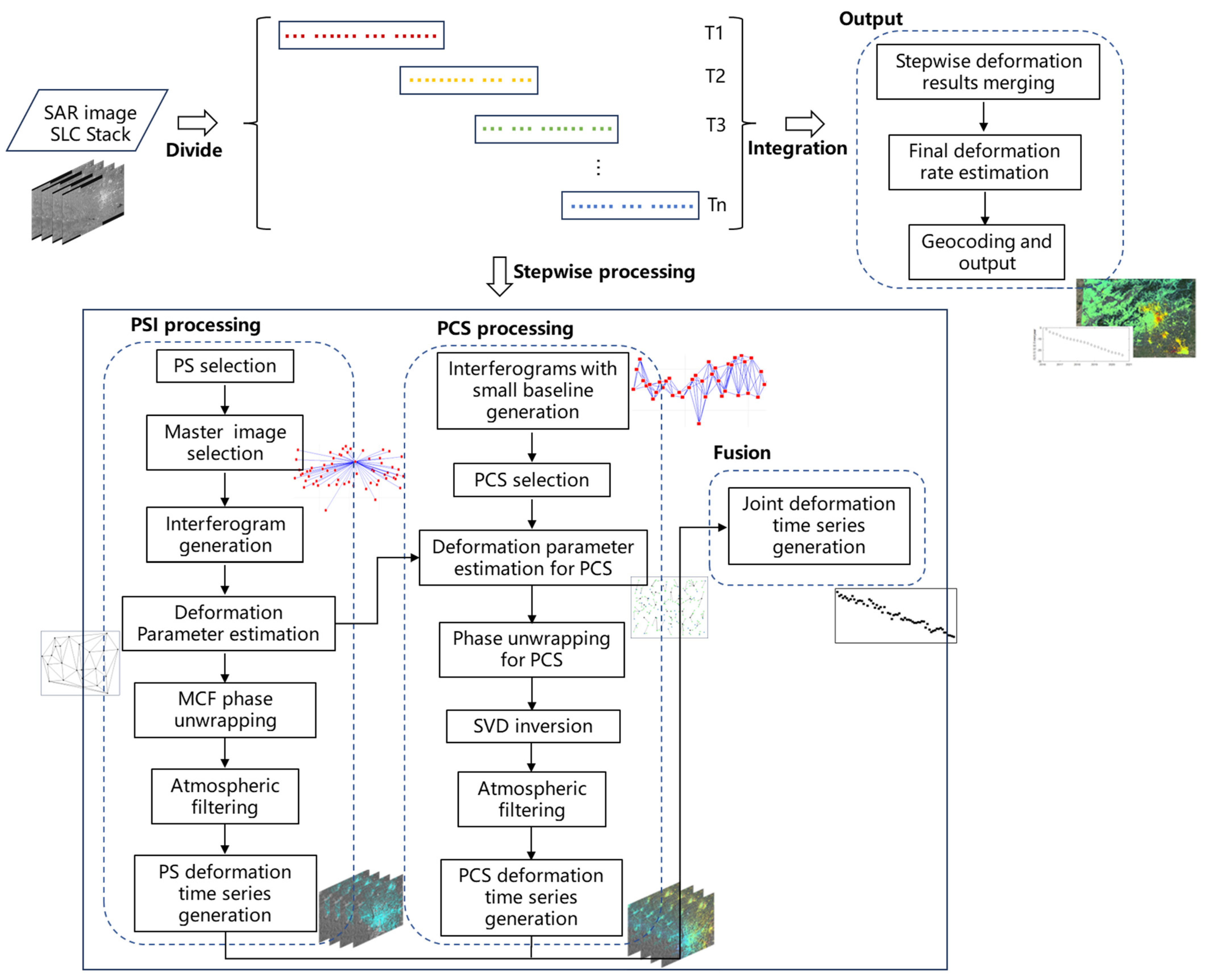
Following standard preprocessing steps, including data conversion and image coregistration, a stack of single-look complex (SLC) images was obtained. The SLC image stack is then divided into several groups in the temporal domain with some overlaps based on using the average coherence distribution of the interferograms. PSI processing was performed on each temporal subset, which can reduce the effect of decorrelation and computation burden in the long time series analysis. Furthermore, small baseline interferograms with a single look were generated in each subset, and the PCSs were selected based on a certain coherence threshold to improve the spatial density of the scatterers. The deformation results of PS are taken as reference points in PCS deformation estimation through PS-SBAS processing because PSI methods can better cope with large atmosphere errors. Finally, the unwrapped phases of the PS and PCS were integrated, and the final deformation time-series data were jointly retrieved. A flowchart of the proposed method is presented in Figure 1.
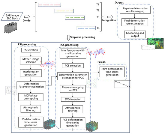
Figure 1.
Flowchart of the proposed SPCS-InSAR method.
2.1. Stepwise PSI Processing
The stepwise method relies on adequately dividing the SAR image stack into several groups in the temporal domain. However, the number of partitioned SAR images should be relatively small to reduce the processing storage burden, eliminate long temporal baselines, and mitigate the effect of the coherence loss of PS. In addition, a sufficient number of SAR images should be available for each group to obtain high-precision PSI deformation results, particularly in regions with large atmospheric turbulence. To maintain the consistency of the estimated results for each subset, some overlaps should exist between adjacent groups to retrieve the joint deformation results. Unlike sequential InSAR estimator methods, the proposed method incorporates temporal overlap with a certain length to maintain processing redundancy and prevent coherent scatterer fading in newly acquired data. With the longer length of the temporal subset, the deformation results are less influenced by atmospheric errors; however, the density of the PS is reduced. Furthermore, the overlap length should not be too long, which increases the computation burden. Therefore, the optimal parameter should be determined by first attempting classical PSI and SBAS methods on the small datasets of the study region.
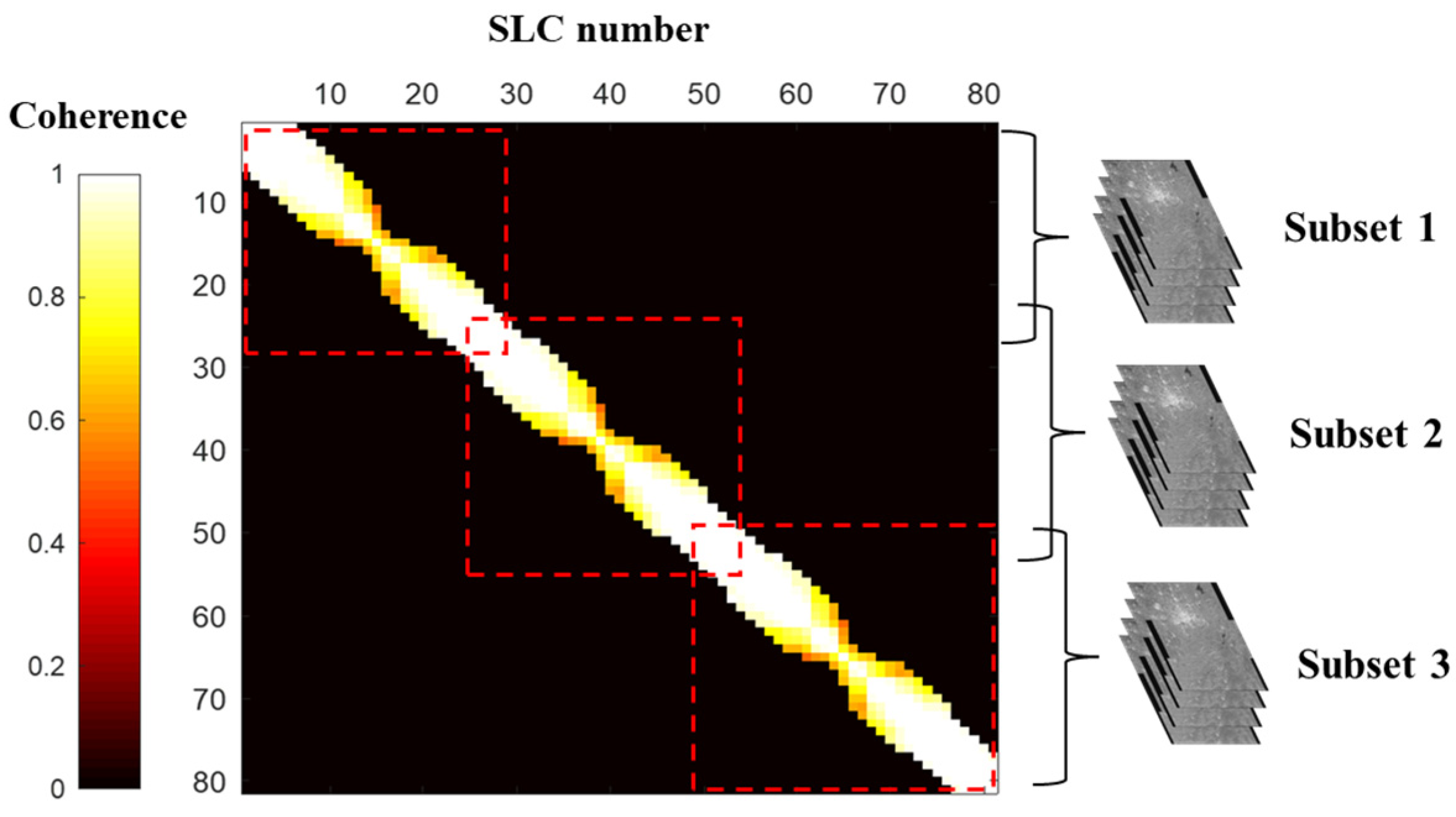
In this study, we select the group method based on the influence of SAR image coherence and atmosphere. The overlap length depends on the atmospheric errors, which guarantees the overall estimation accuracy and processing efficiency. We used 80 SLC images as an example. Figure 2 presents the average coherence of the SAR images. The SAR image stack was grouped into three subsets with overlaps of 4 and 6, and the group boundary lies in the SAR images with high coherence.
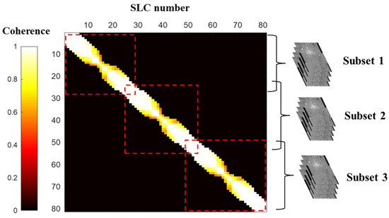
Figure 2.
Group method of the stack of SLC images.
For each temporal subset, classical PSI was used to obtain the deformation results via a time-series analysis of the SLC stack. PSI processing involves the following steps:
- (1)
- PS selection is based on the amplitude-dispersion index (ADI) algorithm, and high-quality scatterers are obtained using a certain ADI threshold.
- (2)
- The topography and flat phases in the interferogram are removed using the external digital elevation model (DEM) and precise orbit file by selecting the master image and generating N interferograms for each pair of master and slave SLC images.
- (3)
- The global reference point in the SAR image is obtained by jointly considering the ADI for the temporal subsets. Then, the deformation parameter estimation is performed on every edge of the PS Delaunay network by analyzing the time-series wrapped differential phase. Linear deformation rates are obtained by integrating the differential parameter with the reference point.
- (4)
- The residual unmodeled wrapped phase is phase unwrapping through the minimum cost flow (MCF) algorithm, followed by atmospheric filtering. The obtained nonlinear deformation phase is added to the linear deformation phase, and the final PS deformation phase time series are generated.
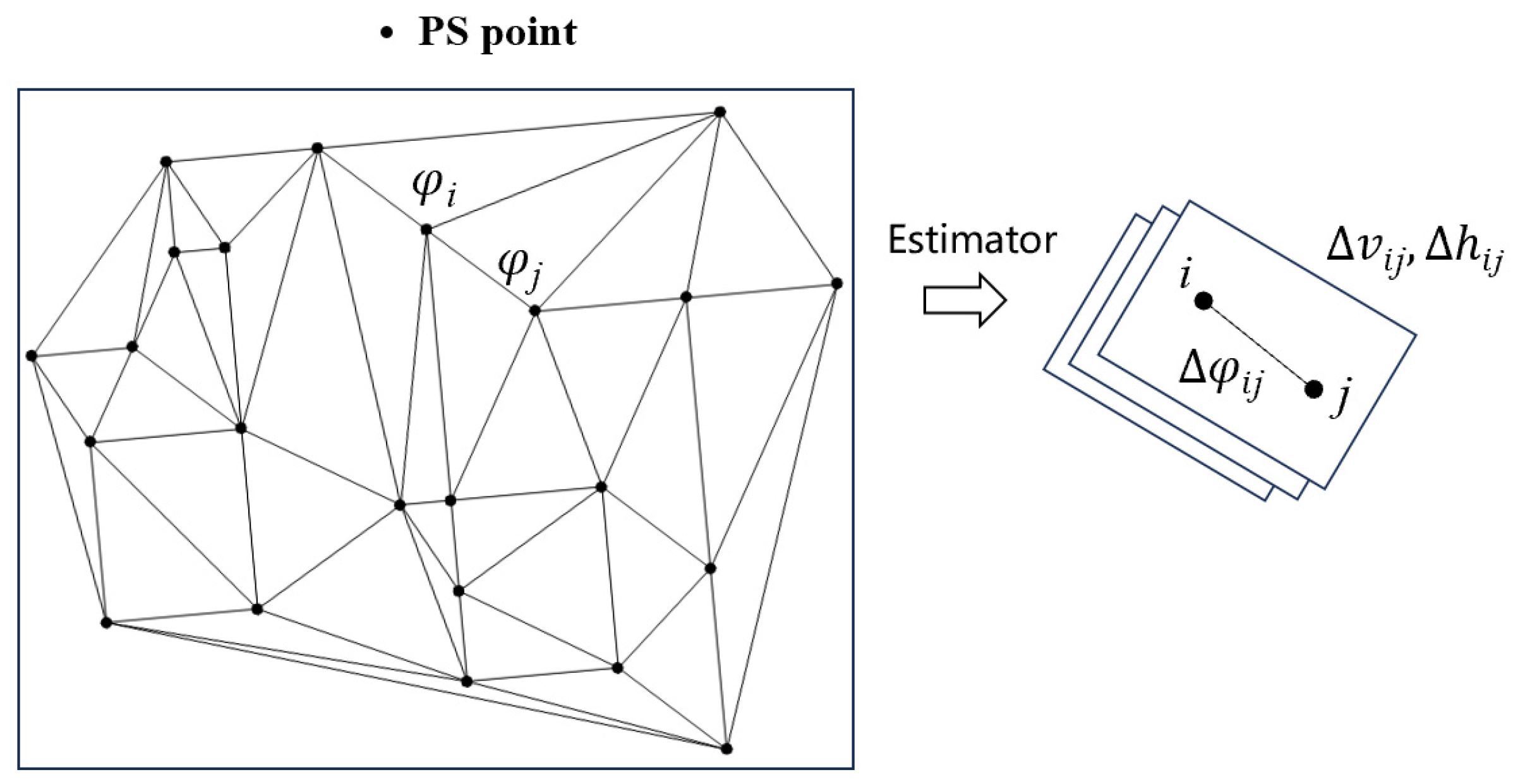
In the deformation estimation step, assuming that Subset M has N + 1 SLC SAR images, an N-wrapped differential interferometric phase is generated in this subset, which can be expressed as {,, …, }. The differential interferometric phase mainly includes the residual topography , deformation , atmospheric , orbit error , and noise phases . While most of the error phases are spatially coherent, they can be mitigated by the phase difference between two adjacent PSs (Figure 3). The differential phase of Scatter i and j can be modeled as the function of the linear deformation rate and residual height using the following expression:
where is the th differential phase, and is the th modeled phase. λ, r, and θ are the radar wavelength, slant range, and incidence angle, respectively. is the spatial perpendicular baseline of th interferometric pair, and is the temporal baseline of th interferometric pair.
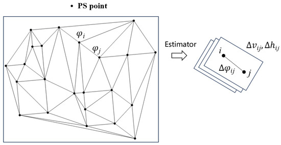
Figure 3.
Deformation parameter estimation using the PSI technique.
As the differential phase is wrapped, the deformation parameter is estimated using the optimization method by minimizing the following object function and iterative searching of the deformation rate and residual height .
2.2. PCS Processing
PSs are usually stable man-made structures that can maintain high coherence over a long period. PCSs are mainly distributed on natural terrain, and they are strongly influenced by seasonal variations, which can only be effective in limited interferometric pairs. The SBASS method employs controlled spatial and temporal baselines to minimize decorrelation effects, making it more suitable for the deformation estimation of unstable PCSs with multireference small baselines interferograms. In addition, the single-look interferograms for PCS were obtained to avoid resolution loss by multi-looking. The PCS selection is then based on the coherence of the interferometric pairs. The coherence value C for the pixel (x, y) in the SAR image can be estimated as follows:
where w is the inverse distance weight, which can reduce the smooth effect of the moving average in coherence calculations, and W is the window length. Spa and Spr are the spatial resolutions of the azimuth and range, respectively. fM and fS are the complex values of the master and slave images for the interferometric pair, respectively.
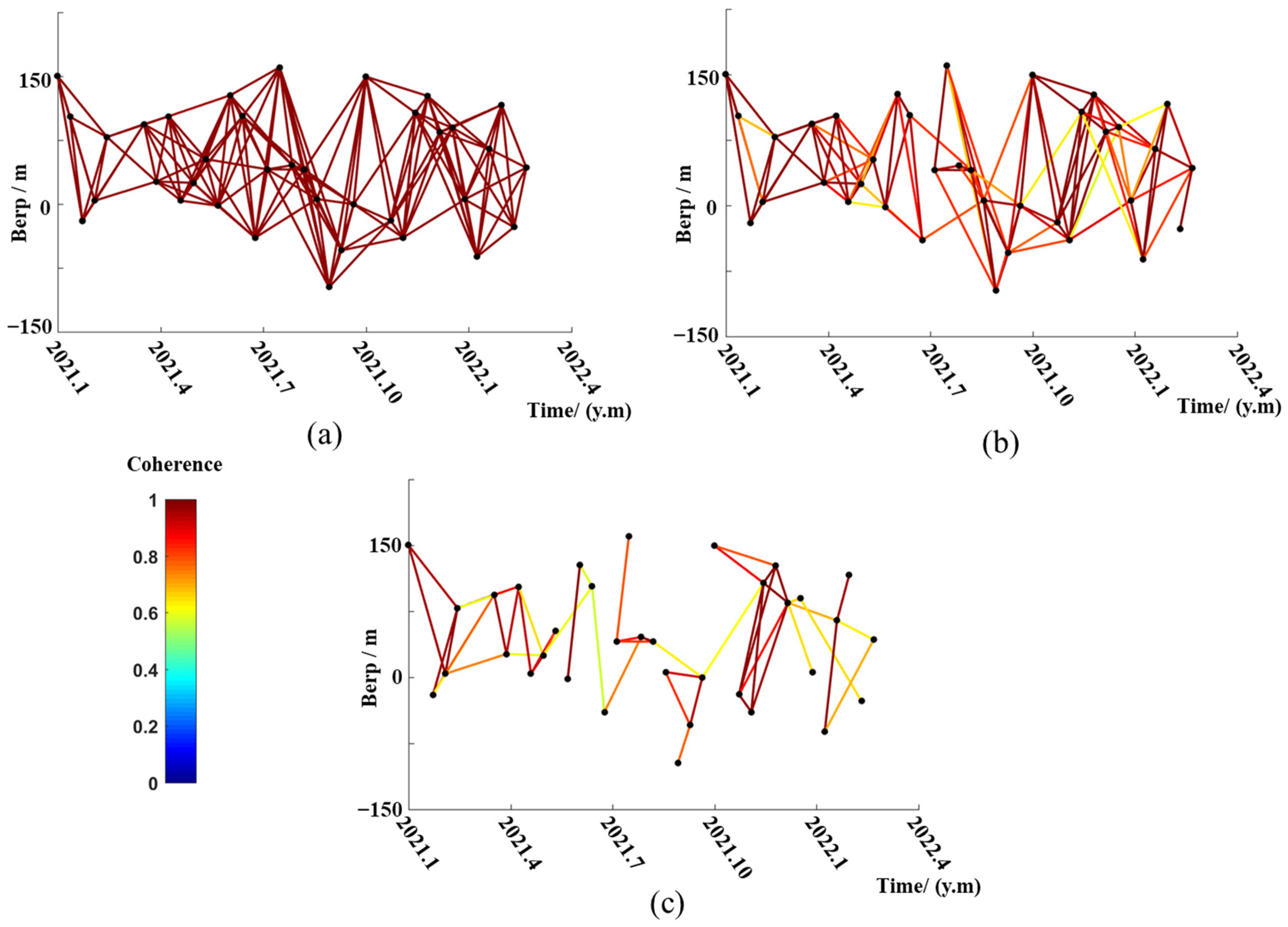
The average coherence for all pixels in the SAR image was calculated, and PCSs were obtained based on the coherence threshold, as well as the effective interferometric pairs for each PCS. The temporal–spatial baseline map of the different scatterers is shown in Figure 4, and the coherence threshold is set to 0.5. The interferograms are categorized into three groups based on coherence properties. The first group comprises PSs acquired from PSI workflow, exhibiting high coherence in all interferograms. The second group is PCSs with high coherence, though some less-coherent interferograms are excluded from this subset. Finally, PCSs with low coherence contain the fewest numbers of interferograms, potentially leading to unconnected or sparse interferometric pairs in some regions.
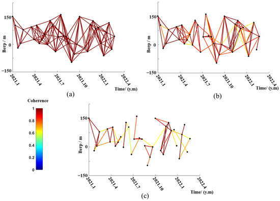
Figure 4.
Interferometric pair distribution for different scatters, (a) PS and (b) PCS with high coherence and (c) PCS with low coherence. The different colored lines represent the coherence value of the scatterer in different interferometric pairs.
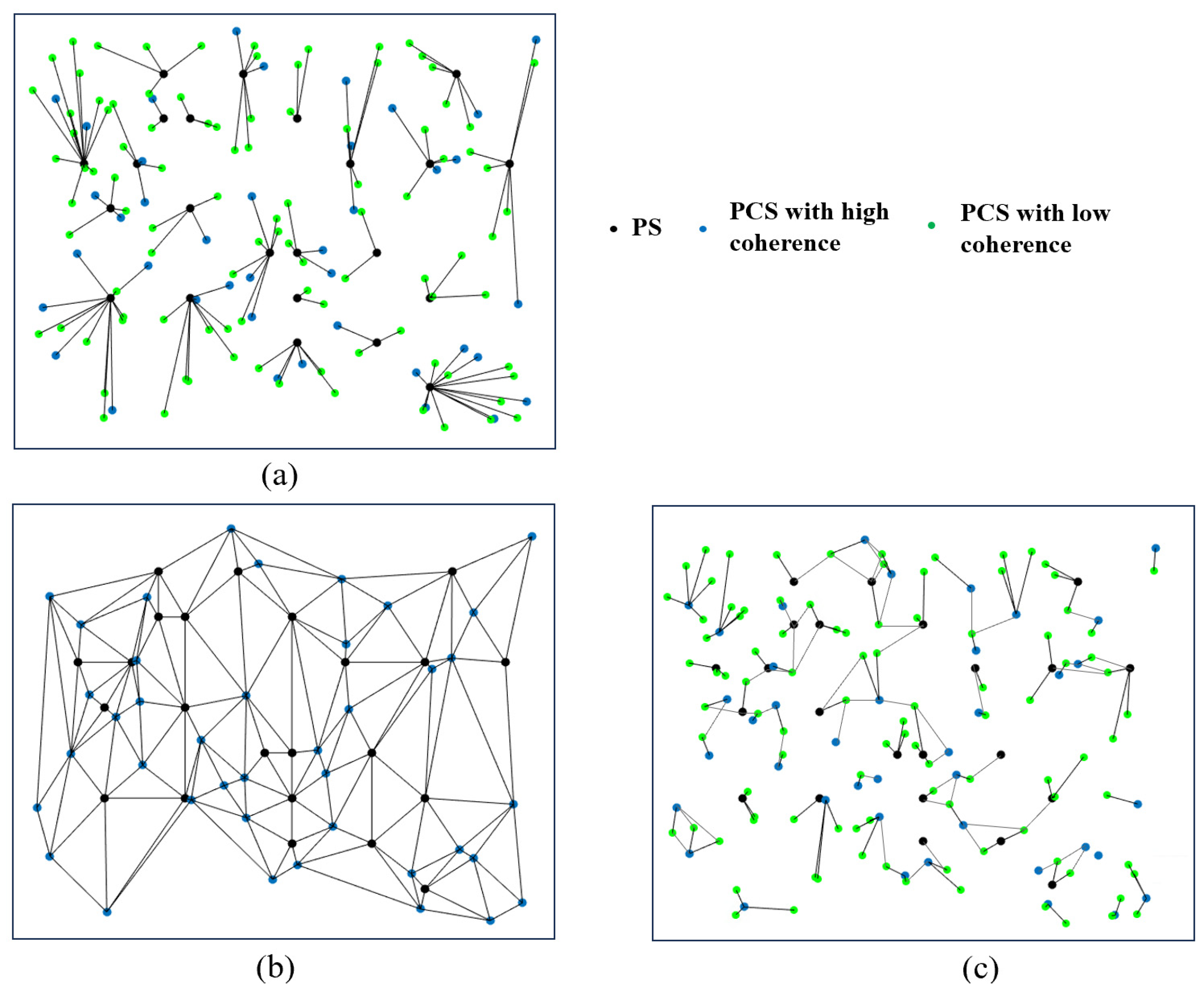
We assume that N + 1 SAR images have generated M interferograms, which can be expressed as = {,, …, }, and PCS only has the subset of PS, . Since PCSs have a limited and varied length of interferograms, these scatterers cannot be directly involved in PSI Delaunay network estimation. In this study, we employed the deformation parameters of PSs in the PSI workflow as a reference network for the estimation of the PCS parameter. The PCSs search the nearby PSs in the surrounding area, and the pair of PCS and PS establish the differential network used to estimate the deformation parameters based on Formula (3) (Figure 5a).
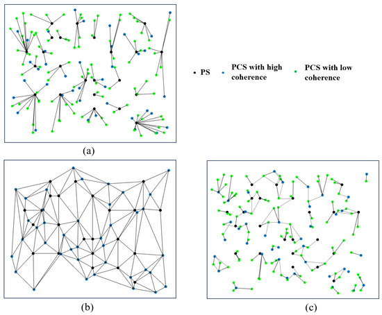
Figure 5.
Deformation estimation in PCS processing, (a) PCS and PS pair network, (b) first network of PS and PCS with high coherence, and (c) second network of PCS with low coherence.
PSs are often sparsely distributed in some natural terrain regions, and PCSs exhibit significant local coherent characteristics. As a result, extremely long arcs can occur between the PCS and its nearest PS, potentially causing large estimation errors. Therefore, we hierarchically solved the PCS parameter estimation, and the two-layer network was used to deal with different kinds of PCS (Figure 5b,c). The PCSs with high coherence were separated from the scatterers using a high coherence threshold, which has enough interferograms in the calculation of parameter estimation and can be integrated with PS as reference deformation values for subsequent scatterers. The PCSs and PSs then form a constraint Delaunay network to avoid long arcs, and only the common interferograms of the two adjacent scatterers were involved in the time series analysis. The PCSs with low coherence in the second network were linked with nearby optimal scatterers by searching adjacent reference scatterers, where the two scatterers have the maximum common interferogram subsets.
Specifically, the two scatterers i and j have two different subsets of and interferograms, respectievely, {,, …, } and {,, …, }. The maximum common subset can be used in the phase difference as Formula (1), and the deformation parameters of the differential networks can be obtained by optimizing the following function:
After calculating all the arcs from the two-layer PCS network, the estimated differential and deformation parameters of PS and PCS can be expressed using the following linear system:
where A is the design matrix of the PCSss with only two nonzero elements 1 and −1 in every row, which defines every arc of the differential network between the PCSs and PSs. Here, R is the design matrix of the reference PS and has one nonzero element 1 for every row, where the column denotes the PS index. B is the estimated differential parameter vector of the network arcs. is the reference deformation parameter vector of the PSs obtained from PSI processing. V is the final deformation parameter vector of the PSs and PCSs, which can be estimated using the least squares solution, as shown in Formula (7).
After obtaining the deformation parameters of all PCSs, the residual wrapped phase of all scatterers with small baseline interferograms was processed by spatial phase unwrapping. For each interferogram, only the wrapped residual phase of the PS and PCS with coherence above the threshold was incorporated into the conventional MCF phase unwrapping with the Delaunay network, which can reduce the unwrapping error propagation from the noisy PCS. Furthermore, for the PCS with coherence below the threshold, a local Delaunay network is connected between the PCS and previous unwrapped scatterers, and the L2-norm least-square phase unwrapping method is used to retrieve the optimized unwrapped phase of the PCS with low coherence. Thus, the unwrapped phase of all scatterers was integrated, and then the deformation phase time series with small baseline interferometric pairs was generated by combining the nonlinear deformation phase and linear deformation rates. The deformation phase time series with small baseline interferometric pairs were then generated and transformed into a common reference of PSI by solving the following equation:
where M is the interferometric design matrix with two nonzero elements, 1 and −1, which defines the index of every interferometric pair. is the unwrapped phase vector of the unwrapped interferograms. is the estimated deformation phase vector.
Equation (8) is solved using singular value decomposition (SVD) inversion. As the different scatterers varied in terms of interferogram lengths, the SVD calculation is performed on the PCS scatterers pixel by pixel. For PCS with low coherence, only the unwrapped phase of the minimum-connected network with the highest coherence was used in SVD calculation. Finally, the cumulative deformation time series of the temporal subset was obtained with the common master reference PSI, and the PSs and PCSs were incorporated into the total deformation results.
2.3. Integration
Stepwise PSI and PCS processing were performed on all temporal subsets of the SAR image stack, and the stepwise deformation time series of different temporal subsets were integrated using the overlap results between adjacent subsets. The common scatterers of different subsets were first confirmed, and those that disappeared in some periods were discarded. The final deformation time series DT can be obtained by integrating the design matrix of each subset:
where S1, S2, …, SN are the design matrix of N temporal subsets, which define the index of the master reference and slave images in PSI processing. D1, D2, …, DN are the corresponding deformation time series vectors of each subset. Linear Equation (9) can be solved using SVD inversion, and the deformation time series of the full temporal coverage and the final linear deformation rate can be obtained. In addition, the SVD calculation is independently performed pixel by pixel, without the need for a large computing burden, like classical PSI, for long-time series SAR image processing. Finally, the deformation results are geocoded and output in the expected file formats.
3. Experiment
3.1. Study Area and Dataset
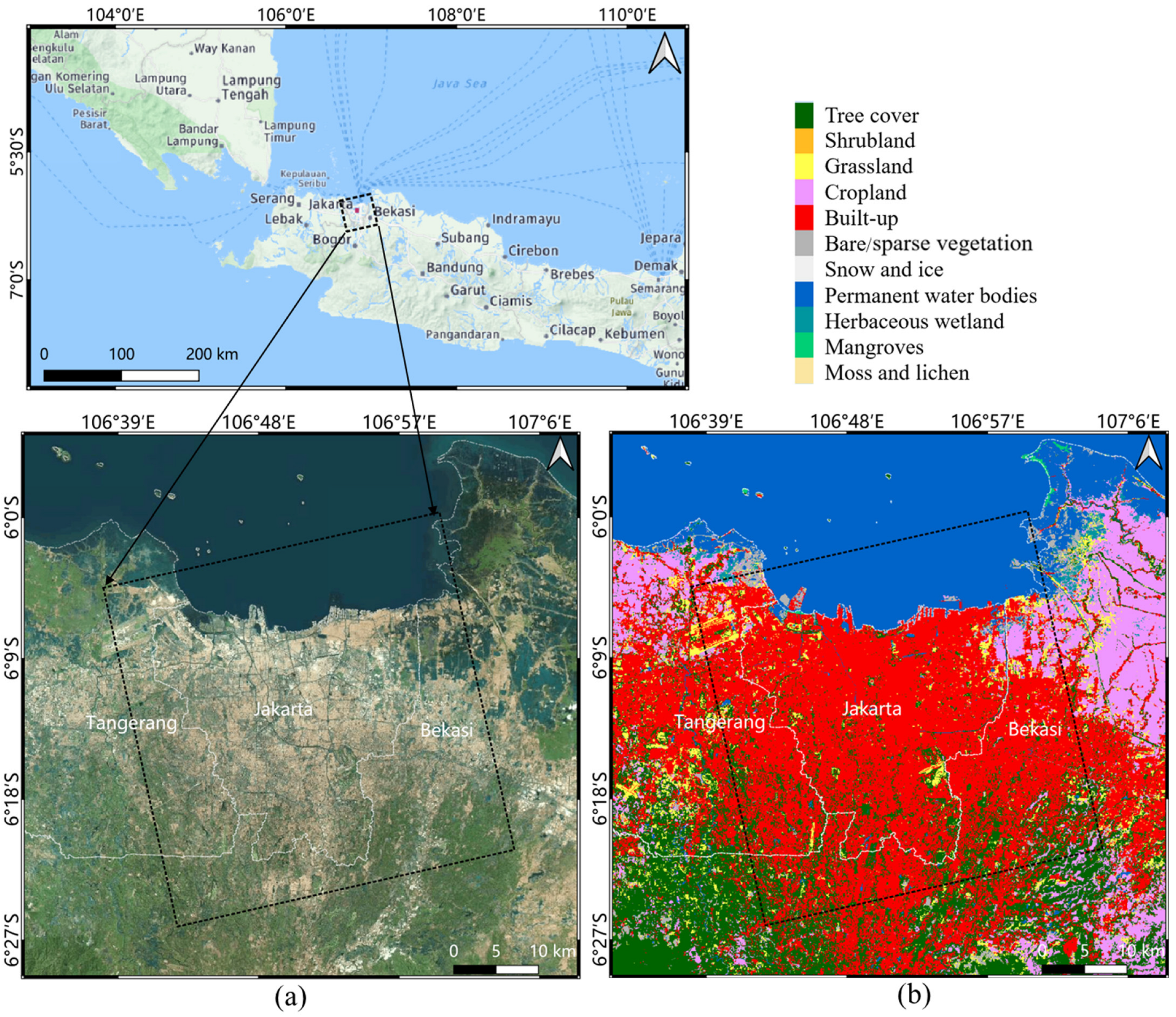
Jakarta is a major city and former capital of Indonesia. It is located in the northwest of Java island and close to the Java Sea in the north, with an average elevation of 7 m above sea level. The location map from Google Optical Satellite data is shown in Figure 6a. With dramatic civilization and population expansion, Jakarta now has an extremely high population density in Asia. Affected by the large amount of water pollution and underground water overexploitation, this area has become one of the world’s most significant subsidence regions [31,32], which are very vulnerable to climate change, sea level rise, and floods. Although Jakarta has a typical tropical rainforest climate, rapid urbanization has prevented rainfall infiltration and groundwater recharge, as shown in the landcover maps in Figure 6b, which are from the European Space Agency (ESA) 2020 Worldcover map [33]. The continuously sinking city has posed a significant threat to urban infrastructures and the social and economic life of Jakarta.
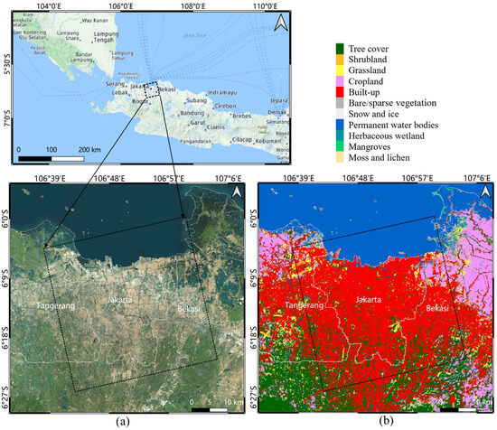
Figure 6.
(a) Location map of Jakarta. (b) Landcover map of Jakarta. The black box is the footprint of the Sentinel-1 SAR image dataset.
To validate our method in the long-time series MT-InSAR analysis, we collected 229 C-band Sentinel-1 ascending SAR images taken between October 2014 and October 2023, with a total data volume of more than 900 GB. Table 1 presents the detailed parameters of the Sentinel-1 dataset. The footprint of the SAR image is shown in Figure 6 with a black box, which covers most of the regions of Jakarta. In addition, an external 30 m DEM AW3d30 was used in the experiment for topographic phase removal and SAR image geocoding of InSAR processing.

Table 1.
Parameters of the SAR image dataset of the study region.
3.2. Results
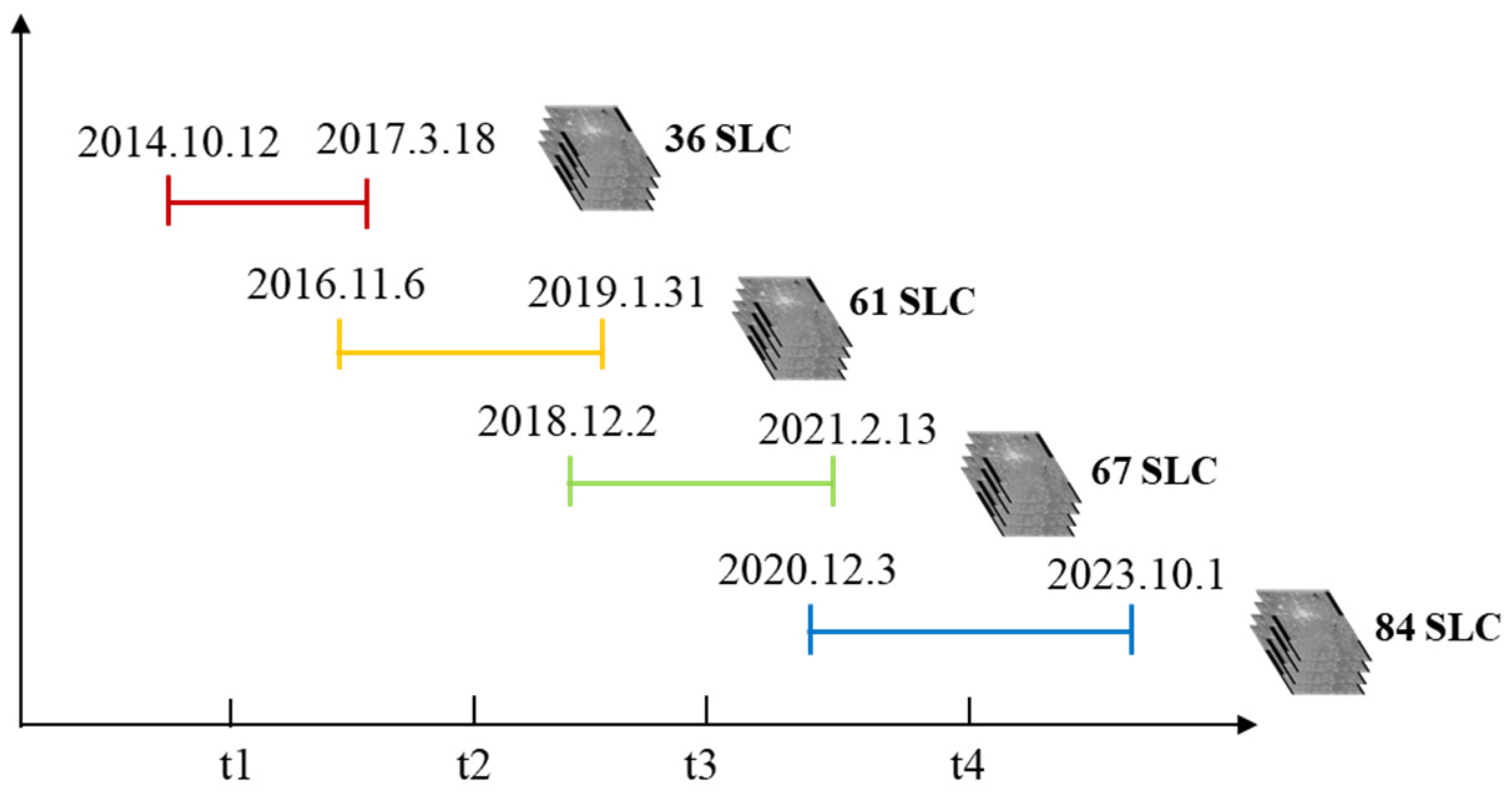
In this experiment, we used the proposed SPCS-InSAR, PSI, DSI, and SBAS methods to process Sentinel-1 SAR images of the study region. The Sentinel-1 SAR image datasets were first imported, and the orbit parameters were updated with precise orbital information. A stack of SLC images was generated by preprocessing the SAR image coregistration with the desired accuracy relative to the common master image. Subsequently, the average coherence distributions for all SLC images were calculated using a multi-looking window of 40 and 8 in the range and azimuth, respectively. The temporal subsets were then grouped based on the coherence and temporal decorrelation. With the consideration of large atmospheric fluctuations in the Jakarta region, 229 SLC image stacks were grouped into 4 subsets with an overlap number of 6. Among them, Subset t1 has 36 SLC images from October 2014 to March 2017, Subset t2 has 61 SLC images from November 2016 to January 2019, Subset t3 has 67 SLC images from December 2018 to February 2021, and Subset t4 has 84 SLC images from December 2020 to October 2023 (Figure 7).
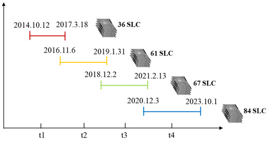
Figure 7.
Shows the temporal subset grouping results for the Sentinel-1 dataset of the study region.
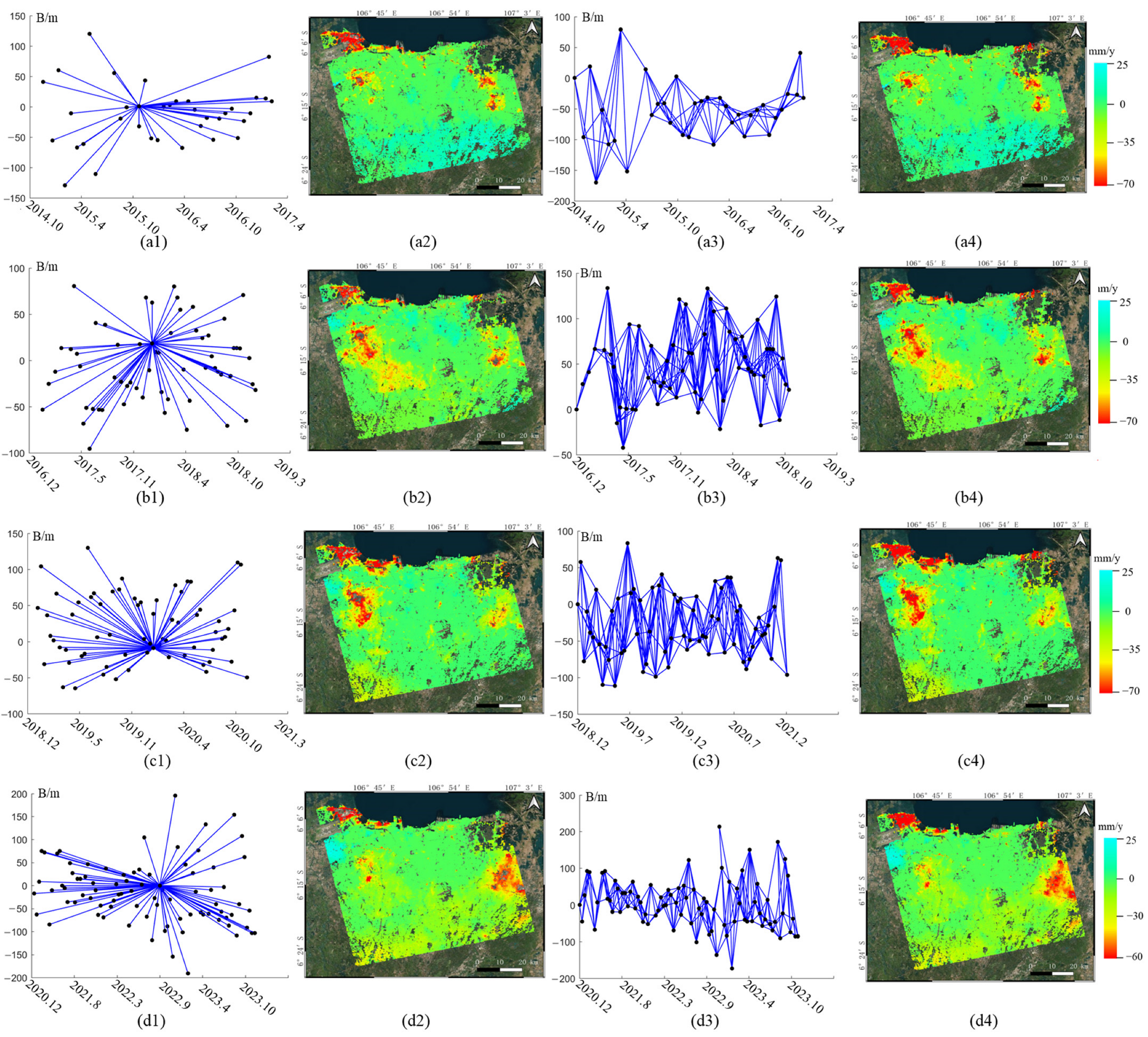
For each subset, PSI processing was first implemented on the SLC stack, and the ADI method was used to select the PS points. The reference image for four subsets is 6 December 2016, 12 January 2018, 26 January 2020, and 5 December 2022. The external DEM was then employed in the topography phase removal and differential interferogram generation. The PS deformation results were obtained individually for 4 subsets. Furthermore, PCS processing begins with the generation of small baseline interferograms. In this experiment, the temporal baseline threshold was set to 60 d, and the spatial perpendicular baseline was 250 m, resulting in 125, 296, 319, and 332 numbers for each interferogram subset, respectively. The coherence and interferograms with a single look were generated with a coherence estimation window size of 5. The PCS selection was based on a coherence threshold of 0.7 and 0.5 for PCSs with high and low coherence, respectively. After parameter estimation for the PCSs and PSs, the two deformation results were combined to generate the deformation rate and displacement time series for the complete SLC stack. The deformation results and temporal–spatial baseline maps of each subset are shown in Figure 8.
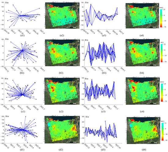
Figure 8.
Temporal–spatial baseline maps and deformation results of PSI and PCS processing for different temporal subsets, (a1–a4) for t1, (b1–b4) for t2, (c1–c4) for t3, and (d1–d4) for t4.
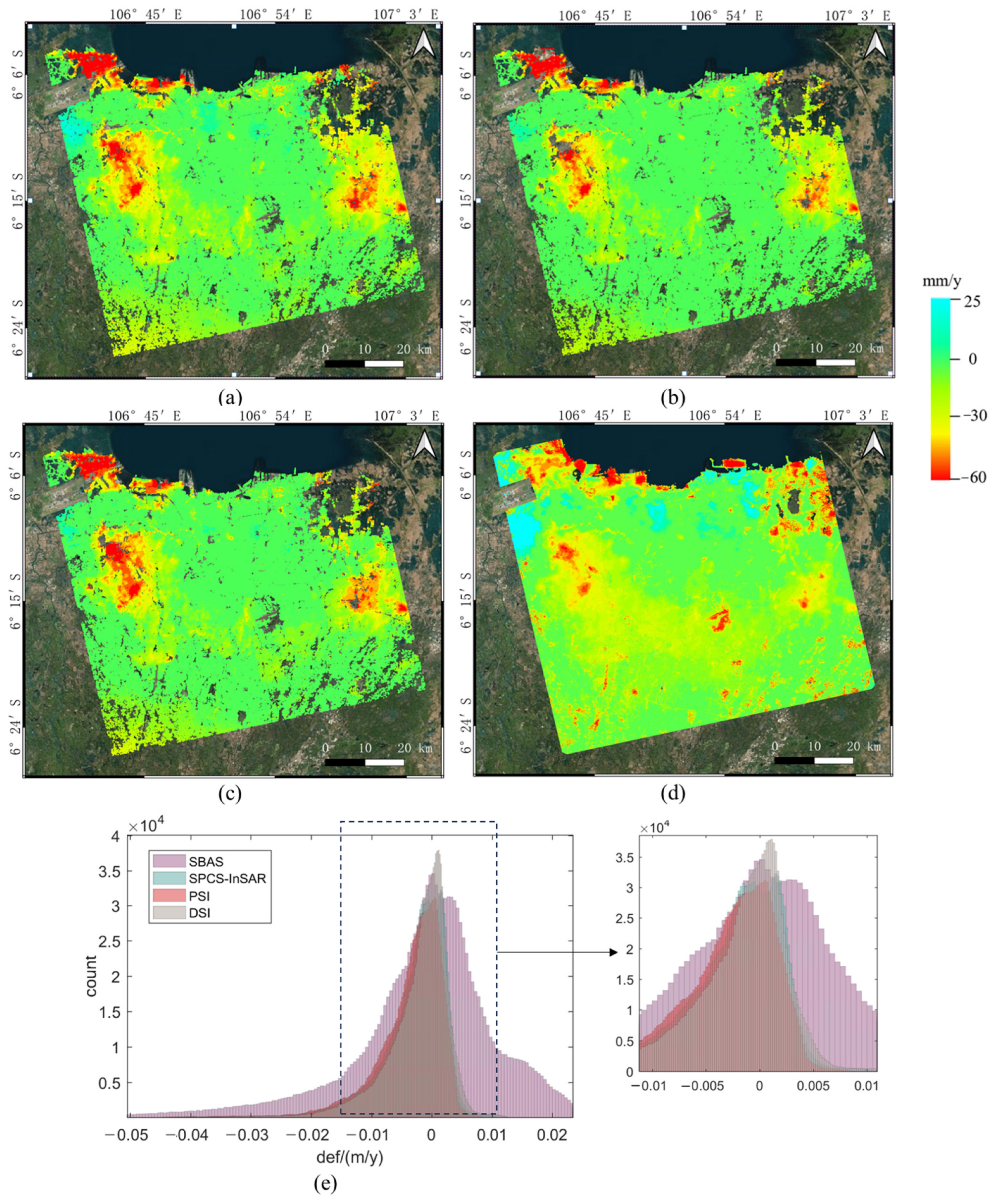
Figure 9 illustrates the final deformation results for the different methods, where (a–d) are the deformation rate maps of the line of sight (LOS) for SPCS-InSAR, PSI, DSI, and SBAS. The results obtained using these methods exhibit similar deformation distribution patterns. Three subsidence bowls exist in the study region, with a maximum subsidence rate of more than 60 mm/y from 2014 to 2023 in the LOS direction. The histogram distributions of the deformation rates of the three methods are shown in Figure 9e, and the standard deviations of the velocity distributions for these methods are 6.02, 5.93, 5.62, and 14.72 mm/y for SPCS-InSAR, PSI, DSI, and SBAS, respectively. The SBAS results demonstrate maximum variance among these methods. The SPCS-InSAR, PSI, and DSI methods have similar deformation results, and they can also be confirmed in the three distributions shown in Figure 9e. In addition, SPCS-InSAR is slightly divergent from the PSI and DSI deformation results. Figure 9d shows that the SBAS results were significantly influenced by atmospheric effects, including the uplift in the northern coastal areas and the topography-related atmosphere in the southern mountainous areas. As Jakarta is located in the coastal areas and borders the Java Sea with the tropical rainforest climate, plenty of rainfall and water vapor exist in the region, causing strong tropospheric phase variation in the interferograms, particularly during the rainy season. SBAS cannot tackle these large errors due to the limitation of small baselines, and the deformation results are strongly affected by atmospheric errors. SPCS-InSAR, PSI, and DSI obtained more significant results than the SBAS method. Moreover, the PSI lost many scatterers in the subsidence center due to the decorrelation of large deformations. DSI slightly improved the deformation estimation results of PSI through adaptive filtering; however, its performance was impaired by long temporal baselines. SPCS-InSAR expanded the deformation results in these regions by stepwise and PCS processing, which increased the density of the scatterers by 8.5% relative to the PSI (SPCS-InSAR: 1528802, and PSI: 1409485). Furthermore, the memory consumption of the SPCS-InSAR and SBAS is less than 32 GB compared with over 100 GB in the PSI and DSI processing. Thus, the SPCS-InSAR method can handle larger amounts of the SAR dataset. The operation on the different subsets in SPCS-InSAR can be processed simultaneously to improve the overall efficiency. With a total processing time of 6.1 h, it outperforms PSI, DSI, and SBAS methods by 8.3 h, 26.5 h, and 11.5 h, respectively. Therefore, the proposed SPCS-InSAR method is effective and efficient for long-time series InSAR processing.

Figure 9.
Deformation rates in the LOS direction of the study region for (a) SPCS-InSAR, (b) PSI, (c) SBAS, and (d) DSI. (e) Histogram of the deformation rates of the three methods.
3.3. Typical Subsidence Analysis
Figure 10a shows the deformation results of SPCS-InSAR in the geological map of the study region. The subsidence in Jakarta is mostly distributed in three regions: Northern Jakarta, Western Tangerang, and Bekasi, with total subsidence areas of more than 100 km2, which is consistent with previous studies. These subsidence centers are all located in densely populated residential areas, as shown in the optical satellite image. Because the geological condition of Jakarta is mainly composed of loose sediments, underground water overexploitation and large-scale construction are the main reasons for city subsidence. The displacement time series results (Figure 10b) demonstrate that the subsidence regions in Jakarta are continuously sinking, with an average cumulative subsidence of over 300 mm from 2014 to 2023. The most serious regions are located in Northern Jakarta coastal areas, which have the largest subsidence rate due to land reclamation. The other subsidence regions exhibited a certain degree of slowing down in recent years, as shown in P2 and P3.
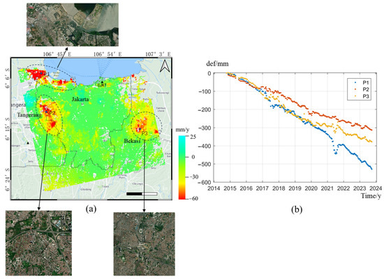
Figure 10.
The subsidence distribution (a) and displacement time series (b) of Jakarta. The black diamond indicates the GNSS station CJKT.
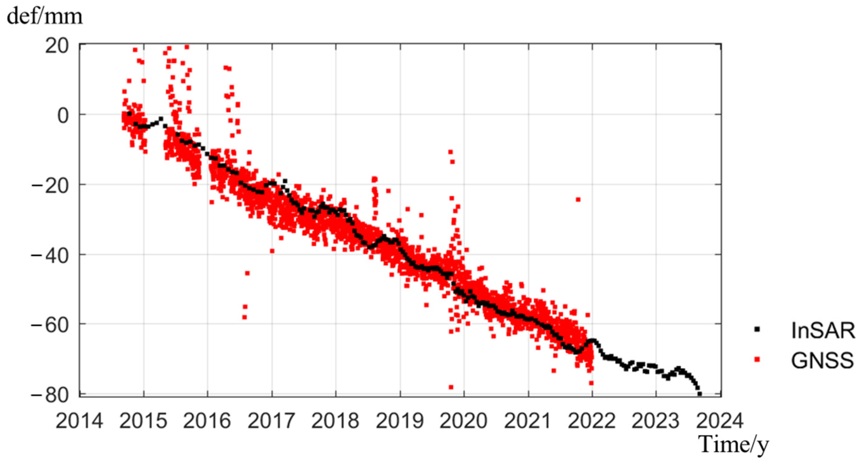
To further validate the accuracy of the SPCS-InSAR deformation results, we used the GNSS measurements in the literature [34] for comparison with nearby InSAR deformation results. Twenty continuous GNSS stations are operational along the coastline of Java island, including the CJKT station in Northern Jakarta, as shown in Figure 10 with the black diamond. The acquired GNSS data were processed using GLOBKv10.75 software, and the daily time series coordinates were obtained. The GNSS measurements of the CJKT recorded precise 3D deformation time series in Jakarta from 2010 to 2021, revealing large velocities in the vertical direction, which is closely related to land subsidence. In this experiment, the GNSS measurements were transformed to the same coordinates of InSAR in the LOS direction. To avoid reference differences between the two observations, the initial offset of the GNSS and InSAR was compared, and the comparison results are illustrated in Figure 11, where the black dot represents the InSAR results, and the red dot represents the GNSS results. The InSAR results demonstrated a similar deformation trend to the GNSS measurements, and the InSAR data exhibited some fluctuations during the acquisition time, which is mainly caused by atmospheric errors. The root mean square error between the two deformation time series is 6.23 mm, which confirms that the InSAR deformation estimation results agree well with GNSS.

Figure 11.
Results of comparison between GNSS and InSAR.
4. Discussion
The massive historical SAR dataset from various satellite systems significantly inspired the InSAR technique in large-scale geodetic applications, particularly for long-term deformation monitoring. Conventional MT-InSAR methods suffer from insufficient scatterers and computational efficiency due to temporal decorrelation and a large computing burden. This study proposed an SPCS-InSAR method that integrates PCS into a stepwise PSI processing workflow to improve the overall deformation precision and processing efficiency. The proposed method first employed stepwise PSI to avoid long temporal baselines by grouping the SAR images in the temporal domain. The PS deformation parameters were taken as the spatial constraint to enhance the estimation accuracy of unstable PCSs with small baseline interferograms by iteratively solving the two-layer differential network of PS and PCS. Finally, it employed the SVD inversion method to link all the temporal subsets based on the overlaps between adjacent groups. In addition, the processing parameters in the proposed method were comprehensively considered. In stepwise processing, the SAR images in the temporal subset should last for 1–2 years to suppress the atmosphere effect, and a larger number of SAR images was used for regions with high coherence. Then, the optimal overlap length was 4–8, considering both processing computation and accuracy. In PCS processing, temporal and spatial baselines ensured sufficient interferograms. Then, the coherence threshold for PCSs was set at 0.4–0.5, ensuring precise MCF phase unwrapping. In addition, the temporal coherence in the deformation estimation was set to 0.7 to maintain the accuracy of the estimated results.
SPCS-InSAR can effectively process long time series of SAR images to retrieve long-term deformation results with more scatterers and high precision to better understand the dynamic deformation process of the Earth’s surface. However, the proposed method has some limitations. First, the different lengths of the temporal subsets and overlaps may influence the deformation estimation results due to atmospheric errors, and they should be adjusted based on practical InSAR data, which relies on processing experience. Second, the accuracy of the SPCSS-InSAR deformation results depends on the PS density of the SAR images, and it is restricted to nonurban and mountainous areas. Finally, the SPCS-InSAR method discarded many scatterers in the farmland and vegetated areas of Northeastern Jakarta (Figure 9a). Thus, the L-band SAR image data (Lutan-1, ALOS-2, and NISAR) should be used to increase the InSAR coherence and PS density in regions with complex terrains. In future work, we will introduce the distributed scatterer into the workflow of SPCS-InSAR to further improve its performance in low-coherence regions.
5. Conclusions
In this study, we propose a stepwise PSI and PCS combined SPCS-InSAR method for long-time deformation monitoring from SAR time series images. The proposed method effectively combines the advantages of current TCS and sequential InSAR methods. By processing the PSI and PCS segmentally, SPCS-InSAR significantly reduces computational and storage consumption compared to conventional methods, thus achieving higher scatterer density and deformation results with higher accuracy. The proposed method uses stepwise PSI processing to alleviate the effect of temporal decorrelation and reduce the computing burden of conventional PSI-based TCS methods. In addition, the overlap length between different temporal groups reduced the error propagation in sequential InSAR processing. The PCS processing with small baseline interferograms complements PS results to significantly improve the scatterer density, particularly in regions with large deformation and natural terrain. Furthermore, SPCS-InSAR obtains more accurate deformation results in regions with large atmospheric turbulence by using PS deformation results as a reference for PCS processing. The proposed method employs sufficient overlap lengths among different temporal subsets to ensure deformation result consistency. The SPCS-InSAR method was validated using a 9-year dataset of 229 Sentinel-1 ascending SAR images in Jakarta from 2014 to 2023. The deformation results were compared with those of classical PSI and SBAS methods. The comparison results demonstrate that the SPCS-InSAR method achieves a balance between deformation estimation accuracy and computing efficiency while increasing the scatterer density of the deformation results by 8.5% in the study region. Thus, the proposed SPCS-InSAR method can be applied well to long-term deformation observations.
Author Contributions
Conceptualization, J.Z., W.D. and X.F.; methodology, J.Z., W.D., X.F. and Y.Y.; validation, X.L., W.D., X.F. and Y.Y.; formal analysis, J.Z.; investigation, J.Z. and W.D.; writing—original draft preparation, J.Z.; writing—review and editing, J.Z., W.D., X.F. and Y.Y.; visualization, J.Z. and W.D.; supervision, project administration, Y.Y. and X.L. All authors have read and agreed to the published version of the manuscript.
Funding
This research was funded by the National Natural Science Foundation of China (grant No. 41801356).
Data Availability Statement
The Setinel-1 dataset was provided by the European Space Agency (ESA). The AW3d30 DEM was provided by JAXA.
Acknowledgments
We greatly thank ESA for providing the Sentinel-1 data.
Conflicts of Interest
The authors declare no conflicts of interest.
References
- Xue, F.; Lv, X.; Yun, Y. A review of time-series interferometric SAR techniques: A tutorial for surface deformation analysis. IEEE Geosci. Remote Sens. Mag. 2020, 8, 22–42. [Google Scholar] [CrossRef]
- Wang, R.; Liu, K.; Liu, D. LuTan-1: An innovative L-band spaceborne bistatic interferometric synthetic aperture radar mission. IEEE Geosci. Remote Sens. Mag. 2024. [Google Scholar] [CrossRef]
- Suzuki, S.; Motohka, T. Overview of ALOS-2 and ALOS-4 L-band SAR. In Proceedings of the 2021 IEEE Radar Conference, Atlanta, GA, USA, 8–14 May 2021; pp. 1–4. [Google Scholar]
- Torres, R.; Snoeij, P.; Geudtner, D.; Bibby, D. GMES Sentinel-1 mission. Remote Sens. Environ. 2012, 120, 9–24. [Google Scholar] [CrossRef]
- Chapman, B.; Anconitano, G.; Borsa, A.; Christensen, A. The NASA ISRO SAR (NISAR) Mission-Validation of Science Measurement Requirements. In Proceedings of the IGARSS 2024, Athens, Greece, 7–12 July 2024. [Google Scholar]
- Festa, D.; Bonano, M.; Casagli, N. Nation-wide mapping and classification of ground deformation phenomena through the spatial clustering of P-SBAS InSAR measurements: Italy case study. ISPRS J. Photogramm. Remote Sens. 2022, 189, 1–22. [Google Scholar] [CrossRef]
- Moretto, S.; Bozzano, F.; Mazzanti, P. The role of satellite InSAR for landslide forecasting: Limitations and openings. Remote Sens. 2021, 13, 3735. [Google Scholar] [CrossRef]
- Moro, M.; Saroli, M.; Stramondo, S.; Bignami, C. New insights into earthquake precursors from InSAR. Sci. Rep. 2017, 7, 12035. [Google Scholar] [CrossRef]
- Li, S.; Xu, W.; Li, Z. Review of the SBAS InSAR Time-series algorithms, applications, and challenges. Geod. Geodyn. 2022, 13, 114–126. [Google Scholar] [CrossRef]
- Ferretti, A.; Prati, C.; Rocca, F. Nonlinear subsidence rate estimation using permanent scatterers in differential SAR interferometry. IEEE Trans. Geosci. Remote Sens. 2000, 38, 2202–2212. [Google Scholar] [CrossRef]
- Berardino, P.; Fornaro, G.; Lanari, R.; Sansosti, E. A new algorithm for surface deformation monitoring based on small baseline differential SAR interferograms. IEEE Trans. Geosci. Remote Sens. 2002, 40, 2375–2383. [Google Scholar] [CrossRef]
- Hooper, A. A multi-temporal InSAR method incorporating both persistent scatterer and small baseline approaches. Geophys. Res. Lett. 2008, 35, 1–5. [Google Scholar] [CrossRef]
- Teixeira, A.; Bakon, M.; Perissin, D.; Sousa, J. InSAR Analysis of Partially Coherent Targets in a Subsidence Deformation: A Case Study of Maceió. Remote Sens. 2024, 16, 3806. [Google Scholar] [CrossRef]
- Zhang, L.; Lu, Z.; Ding, X.; Jung, H. Mapping ground surface deformation using temporarily coherent point SAR interferometry: Application to Los Angeles Basin. Remote Sens. Environ. 2012, 117, 429–439. [Google Scholar] [CrossRef]
- Hu, F.; Wu, J.; Chang, L.; Hanssen, R. Incorporating temporary coherent scatterers in multi-temporal InSAR using adaptive temporal subsets. IEEE Trans. Geosci. Remote Sens. 2019, 57, 7658–7670. [Google Scholar] [CrossRef]
- Dörr, N.; Schenk, A.; Hinz, S. Fully integrated temporary persistent scatterer interferometry. IEEE Trans. Geosci. Remote Sens. 2022, 60, 4412815. [Google Scholar] [CrossRef]
- Shahryarinia, K.; Omidalizarandi, M.; Heidarianbaei, M.; Sharifi, M.; Neumann, I. Detecting change points in time series of inSAR persistent scatterers using deep learning models. Appl. Geomat. 2025, 1–10. [Google Scholar] [CrossRef]
- Wassie, Y.; Milillo, P. Interferometric Synthetic Aperture Radar Multitemporal Deformation Monitoring: A review of machine learning techniques. IEEE Geosci. Remote Sens. Mag. 2025, 2–26. [Google Scholar] [CrossRef]
- Chen, C.; Dai, K.; Tang, X.; Cheng, J.; Pirasteh, S.; Wu, M.; Shi, X.; Zhou, H.; Li, Z. Removing InSAR Topography-Dependent Atmospheric Effect Based on Deep Learning. Remote Sens. 2022, 14, 4171. [Google Scholar] [CrossRef]
- Sun, X.; Zimmer, A.; Mukherjee, S.; Kottayil, N.K.; Ghuman, P.; Cheng, I. DeepInSAR—A Deep Learning Framework for SAR Interferometric Phase Restoration and Coherence Estimation. Remote Sens. 2020, 12, 2340. [Google Scholar] [CrossRef]
- Ren, P.; Han, Z.; Yu, Z.; Zhang, B. Confucius tri-learning: A paradigm of learning from both good examples and bad examples. Pattern Recognit. 2025, 163, 111481. [Google Scholar] [CrossRef]
- Tiwari, A.; Narayan, A.; Dikshit, O. Deep learning networks for selection of measurement pixels in multi-temporal SAR interferometric processing. ISPRS J. Photogramm. Remote Sens. 2020, 166, 169–182. [Google Scholar] [CrossRef]
- Ma, P.; Yu, C.; Jiao, Z.; Zheng, Y.; Wu, Z. Improving time-series InSAR deformation estimation for city clusters by deep learning-based atmospheric delay correction. Remote Sens. Environ. 2024, 304, 114004. [Google Scholar] [CrossRef]
- Zhou, L.; Yu, H.; Lan, Y.; Xing, M. Deep Learning-Based Branch-Cut Method for InSAR Two-Dimensional Phase Unwrapping. IEEE Trans. Geosci. Remote Sens. 2022, 60, 5209615. [Google Scholar] [CrossRef]
- Ansari, H.; De Zan, F.; Bamler, R. Sequential estimator: Toward efficient InSAR time series analysis. IEEE Trans. Geosci. Remote Sens. 2017, 55, 5637–5652. [Google Scholar] [CrossRef]
- Wang, B.; Zhang, Q.; Zhao, C.; Pepe, A.; Niu, Y. Near real-time InSAR deformation time series estimation with modified Kalman filter and sequential least squares. IEEE J. Sel. Top. Appl. Earth Obs. Remote Sens. 2022, 15, 2437–2448. [Google Scholar] [CrossRef]
- Xu, J.; Jiang, M.; Ferreira, V.; Wu, Z. Time-series InSAR dynamic analysis with robust sequential adjustment. IEEE Geosci. Remote Sens. Lett. 2022, 19, 4514405. [Google Scholar] [CrossRef]
- Liu, J.; Hu, J.; Li, Z.; Zhang, L. Dynamically estimating deformations with wrapped InSAR based on sequential adjustment. J. Geod. 2023, 97, 49. [Google Scholar] [CrossRef]
- Wang, Y.; Cui, X.; Che, Y. Near Real-Time Monitoring of Large Gradient Nonlinear Subsidence in Mining Areas: A Hybrid SBAS-InSAR Method Integrating Robust Sequential Adjustment and Deep Learning. Remote Sens. 2024, 16, 1664. [Google Scholar] [CrossRef]
- Lv, X.; Yazıcı, B.; Zeghal, M.; Bennett, V.; Abdoun, T. Joint-scatterer processing for time-series InSAR. IEEE Trans. Geosci. Remote Sens. 2014, 52, 7205–7221. [Google Scholar]
- Bakr, M. Influence of groundwater management on land subsidence in deltas: A case study of Jakarta (Indonesia). Water Resour. Manag. 2015, 29, 1541–1555. [Google Scholar] [CrossRef]
- Abidin, H.; Andreas, H.; Gumilar, I. Land subsidence of Jakarta (Indonesia) and its relation with urban development. Nat. Hazards 2011, 59, 1753–1771. [Google Scholar] [CrossRef]
- Zanaga, D.; Van De Kerchove, R.; De Keersmaecker, W. ESA WorldCover 10 m 2020 v100 [Data Set]; Universitat Politècnica de València: Valencia, Spain, 2020. [Google Scholar] [CrossRef]
- Susilo, S.; Salman, R.; Hermawan, W. GNSS land subsidence observations along the northern coastline of Java, Indonesia. Sci. Data 2023, 10, 421. [Google Scholar] [CrossRef] [PubMed]

Disclaimer/Publisher’s Note: The statements, opinions and data contained in all publications are solely those of the individual author(s) and contributor(s) and not of MDPI and/or the editor(s). MDPI and/or the editor(s) disclaim responsibility for any injury to people or property resulting from any ideas, methods, instructions or products referred to in the content. |
© 2025 by the authors. Licensee MDPI, Basel, Switzerland. This article is an open access article distributed under the terms and conditions of the Creative Commons Attribution (CC BY) license (https://creativecommons.org/licenses/by/4.0/).