Abstract
Identified as early as 2000, the challenges involved in developing and assessing remote sensing models with small datasets remain, with one key issue persisting: the misuse of random sampling to generate training and testing data. This practice often introduces a high degree of correlation between the sets, leading to an overestimation of model generalizability. Despite the early recognition of this problem, few researchers have investigated its nuances or developed effective sampling techniques to address it. Our survey highlights that mitigation strategies to reduce this bias remain underutilized in practice, distorting the interpretation and comparison of results across the field. In this work, we introduce a set of desirable characteristics to evaluate sampling algorithms, with a primary focus on their tendency to induce correlation between training and test data, while also accounting for other relevant factors. Using these characteristics, we survey 146 articles, identify 16 unique sampling algorithms, and evaluate them. Our evaluation reveals two broad archetypes of sampling techniques that effectively mitigate correlation and are suitable for model development.
1. Introduction
In the field of remote sensing, image-based datasets typically contain a limited number (tens to hundreds) of large images (thousands of pixels) that represent contiguous portions of the Earth’s surface. These datasets are utilized to develop automated labeling techniques for the vast amounts of unlabeled data generated by remote sensing imaging systems in use for practical applications. A primary method for automated labeling is the supervised training of machine learning models. These models require a significant number of observations to learn the mapping between data and labels. Furthermore, these models also make the pragmatic choice of working with image sizes ranging in the tens to hundreds of pixels to reduce computational burden and conform to model constraints. Sampling methods are employed to generate these observations from the datasets, meeting the necessary criteria for effective model training.
Outside the field of remote sensing, image-based datasets for classification and segmentation typically contain many (thousands to millions) small images (ranging from 64 × 64 to 512 × 512 pixels) that are independent and non-contiguous. Because the images are independent and non-contiguous, the sampling process can treat each image as an independent observation, and partitioning of observations into test and training sets is straightforward. Even the most basic methods (e.g., random sampling) produce training and testing sets suitable for model development. In the field of remote sensing, similar sampling methods have often been applied inappropriately. Simple methods are inappropriate because the observations are not independent; they are, in fact, sub-regions, which are part of a contiguous larger image. As many previous studies have highlighted, using these methods can introduce a high level of correlation between observations in the training and testing samples. This correlation can result in biased estimates of generalization error during the model development process.
In a seminal 2000 article, Friedl et al. [1] first recognized the issue of local spatial autocorrelation in remote sensing imagery and its effects on estimated generalization errors. This issue was revisited in 2013, when Zhen et al. [2] continued investigating the effects of dependence between training and testing samples. The issue, induced by the employed sampling methodology, was presented as well as the resulting effects on generalization error estimates. Zhou et al. [3] were the first to recognize that two types of correlation exist, namely, the local spatial autocorrelation identified by Friedl et al. [1] and the overlap between the spatial extents of observations in the training and testing samples. In 2017, Liang et al. [4] provided a strong theoretical argument rooted in computational learning theory, describing how these correlations bias generalization error. Liang et al. [4] further provided statistical measurements of the local spatial autocorrelation of pixel spectra and empirical evidence of the correlation’s effects on empirical error. Similarly, in 2017, Hansch et al. [5] joined Liang et al. to introduce some of the first methodological improvements to mitigate these issues.
One of the most impactful results was provided by Lange et al. [6]; in 2018, they generated empirical results showing that sampling methodologies resulting in high levels of spatial correlation can enable even the simplest models to appear to achieve performance comparable to state-of-the-art methods. In their work, a small convolutional neural network (CNN) model with approximately 500k parameters was trained using a sampling method that allowed correlation and one that mitigated it. When trained with the sampling method, which mitigated correlation (using 30% of the dataset for training), the model achieved a Cohen’s kappa () value of 0.2. When training with the sampling method, which allowed correlation the model achieved above . The reported state-of-the-art method [7] at the time achieved with the same percentage of training data, showing that inappropriate sampling methods can have a phenomenal impact during the model assessment. After the presentation of these findings, many researchers [8,9,10,11] have reiterated and strengthened the evidence of the risks of using simple random sampling methodologies for remote sensing model development, specifically from size-constrained datasets.
1.1. Model Development Theory
The application of sampling algorithms to remote sensing imagery is effective in generating multiple observations of a desired size and in creating training and testing samples, which are essential for the model development process. This process involves training a model to represent a mapping from the input space X to the output space Y in the form of a hypothesis, . Observations are drawn from a true distribution, D, to form a dataset with an empirical distribution, . However, the true distribution of remote sensing data is typically unknowable because a single data collection event rarely captures all possible observations for the given set of intrinsic and extrinsic conditions. In simpler terms, collecting enough data to fully represent every possible scenario under the same conditions is often impractical, cost-inefficient, or even impossible. As a result, the dataset reflects only a limited sample of the true distribution.
The objective of model training is to learn an h that minimizes the error when applied to new samples drawn from D. However, due to the unknowable nature of D, it is impossible to measure this generalization error directly. In practice, to estimate model performance on new data from D, the dataset is sampled to create training T and testing S samples. A model is trained on T, and its performance is evaluated using S to obtain an empirical error. If S is identically and independently distributed (i.i.d.) with respect to , the empirical error can provide an unbiased estimate of the model’s generalization error.
The assumption that S is i.i.d. with respect to ensures that the testing sample S is representative of the empirical distribution, allowing for an unbiased estimate of the generalization error. However, this assumption pertains primarily to the relationship between S and and does not inherently restrict the relationship between T and S. If a correlation exists among observations in the underlying distribution, the sampling process can propagate this correlation between T and S. Thus, while a sampling process may aim to create an i.i.d. S, it does not always guarantee independence between T and S. A dependence between T and S can lead to a biased estimate of the generalization error, as T may contain information present in S. This scenario can be viewed as a form of data leakage.
1.2. Model Assessment with Correlated Samples
The interrelationships between , T, and S significantly influence the process of assessing a model’s generalizability. In an idealized scenario, T and S are both i.i.d. with respect to , and T and S are independent. When T is representative of , a learned h should generalize well to . Furthermore, this can be empirically determined using S, as it is also representative of and independent of T. This independence ensures that the evaluation of h on S is not biased by the data used during training, thereby providing an unbiased estimate of the model’s generalization performance.
However, when correlation exists among the observations in , the interrelationships between T, S, and become more complex, particularly if the sampling process does not adequately account for this correlation. While the relationship between T and S with may deviate from the i.i.d. assumption and introduce bias into the empirical error (note: this concept is potentially related to exchangeability and de Finetti’s theorem [12,13]. If slices of a contiguous image can be shown to be exchangeable, then breaking the i.i.d. assumption may have a reduced impact on empirical error bias), we posit that the relationship between T and S has the greatest impact on the assessment of generalizability.
When T and S are highly correlated, it becomes challenging, if not impossible, to determine whether h has simply memorized the observations from T by recalling for a given from S during testing, or if h has learned the underlying patterns in T and can generalize when predicting a y for a given x from S. The independence of T and S ensures that h cannot rely on memorization of samples seen in T when tested on S. Therefore, the empirical error calculated when T and S have low correlation is more indicative of the model’s generalizability.
Even when either or both T and S are not i.i.d. with respect to , it is still possible to assess generalizability, albeit with limitations. If S is not representative of , the assessment will reflect generalization with respect to the distribution of S, rather than . Similarly, if T is not representative of , h may not learn the underlying patterns of , leading to potentially low empirical error on S but limited generalization capability towards .
In summary, when T and S are highly correlated, the empirical error cannot provide a meaningful assessment of a model’s generalizability. However, even if T and S are not i.i.d. with , some information about a model’s generalizability can still be gleaned. This analysis underscores the importance of prioritizing the independence of T and S over their strict adherence to the i.i.d. assumption with . This hypothesis is particularly relevant when designing sampling methods for remote sensing imagery.
1.3. Sampling in Remote Sensing
Within the context of remote sensing, the sampling process aims to create observations and assign them to either the training or testing sample. These observations, commonly referred to as “patches”, are created by “slicing” an image (and its corresponding labels) to select a subcomponent of it. Patches typically range in size from 3 × 3 to 21 × 21 pixels and are generally square with odd dimensions. This ensures no directional bias in the spatial information and provides a well-defined center. This “center pixel location” (CPL) is used to precisely locate patches within the image. The creation of patches involves selecting these CPLs using a sampling algorithm and slicing a patch of the defined size around each CPL.
As we show in our results, stratified random sampling (note: we later refer to this as ’Random Stratified’) is one of the most commonly applied sampling methods. It starts by grouping all pixels in the dataset based on their label, resulting in a stratum per label. Typically, 10–25% of the pixels in each stratum are randomly selected for the training sample, with the remainder going to the testing sample. Patches of the predetermined size are then extracted from the imagery using the pixel locations in the training and testing samples as the patches’ CPLs.
Stratified sampling is designed to produce a sample that is i.i.d. with . However, when applied to spatial data with inherent spatial autocorrelation [3,4], the resulting T may not be i.i.d. with . Furthermore, the testing set is not sampled from , instead, it is formed as the complement of T, comprising all labeled pixels not selected for T. As a result, S may also not be i.i.d. with . Furthermore, the manner of usage of stratified sampling does not consider the relationship between T and S and a large amount of the correlation present can be propagated between them.
The first form of correlation arises from directly overlapping patches that fall into opposite T or S samples. For example, if a patch with size is centered at the CPL and placed into sample T, then all CPLs within P distance will partially overlap (to account for the entire patch area, including the corners, we use axis-specific distance checks). For a rectangular patch, the minimum non-overlapping distance is along the x-axis and along the y-axis. If these neighboring patches are all assigned to T, there is no possibility of overlap. However, if any of these neighboring patches are assigned to S then spatial correlation between T and S will be present. Zhou et al. [3] and Liang et al. [4] showed that depending on the patch size, dataset imagery size, and training-to-testing set ratio, this spatial overlap can reach 100%. In general, the larger the patch size, the greater the likelihood that overlap correlation will exist, both because larger patches cover more spatial area and because the total area of the dataset imagery does not increase in proportion.
The second form of correlation is due to the local spatial autocorrelation present in remote sensing imagery, where the spectra (and labels) of adjacent pixels tend to be highly correlated. Both Friedl et al. [1] and Liang et al. [4] provided empirical evidence that pixels near each other tend to have a high degree of correlation. Furthermore, it is theoretically evident that neighboring pixels in remote sensing imagery are highly correlated due to the spatial resolution of the imaging sensors, which captures objects larger than a single pixel, and the point spread function of the sensors, which causes signal spillover into adjacent pixels. As a result, if a patch is placed into T and its closest non-overlapping neighbor(s) are placed into S, some amount of spatial correlation will exist between T and S. Nalepa et al. [9] provided empirical evidence using both 1D and 3D CNNs, showing that even without spatial information present in patches (e.g., in a 1D CNN), random sampling methods can still induce spatial correlation between T and S, and result in biased estimates of model generalizability.
1.4. Correlation Mitigation
Regardless of the size of the dataset, the contiguous and non-independent nature of the imagery collected will always present some possibility of correlation in the underlying data distribution. However, as the size of the dataset increases the effects of this correlation on the creation of T and S lessen. Logically, the collection of more data under the same intrinsic and extrinsic conditions present for initial data collection is the best form of mitigation. However, collecting more data under the same conditions is often impractical, cost-inefficient, or even impossible. Thus, researchers generally must accept the constraints presented by the size of the dataset(s) and the inherent contiguous nature of it. To that end, as noted, previous works have described sampling methodologies that aim to mitigate or reduce the correlation propagated by the sampling process itself.
We refer to sampling methods that explicitly aim to mitigate correlation as controlled-type sampling methods (credit to Liang et al. [4] for the use of the term “controlled”). These methods systematically select the locations of training and testing CPLs to reduce local spatial autocorrelation and overlap correlation. Generally, controlled-type sampling methods use clustering approaches to select CPLs. By clustering the locations for either or both the training and testing sets, the local spatial autocorrelation at the cluster boundaries can be lower than what is achieved through random sampling approaches, as we will demonstrate in later sections. Additionally, by enforcing a minimum distance of the patch size P between CPLs in different sets (training or testing), overlap correlation can be effectively reduced to zero.
Ironically, this systematic selection of CPLs inherently breaks the i.i.d. assumption of model assessment. Whereas random-type sampling approaches, like stratified sampling, attempt to generate an i.i.d. T, controlled-type methods do not. However, what they gain is a markedly lower correlation between the resulting T and S samples. This allows them to mitigate correlation in a holistic approach, trading i.i.d.-ness for lower correlation, and redirection towards the status quo of model development and assessment.
1.5. Overview and Contributions
Certain kinds of sampling methods can cause issues with the propagation of correlation across T and S, which should be otherwise mutually exclusive. In the field of remote sensing, this issue has been pervasive for at least two decades. Many previous works have identified this challenge and proposed mitigation strategies. However, an alarming percentage of the works surveyed have not recognized or implemented any of these mitigation techniques. A comprehensive survey and review of sampling algorithms will help characterize the extent of the issue in current research. Such a review defines the issues and helps identify alternative sampling algorithms and techniques with a broader set of desirable characteristics to give future researchers more options than those provided in previous work. To that end, our work makes the following contributions:
- A survey of the sampling algorithms used in remote sensing model development.
- A set of desirable characteristics to measure in prospective sampling algorithms.
- An evaluation of the set of sampling methods using the desirable characteristics.
- A method for visually representing the results of sampling through footprint plots.
Despite the contributions of our work, it does have limitations. The main limitations lie in (1) the unavoidable bias of the process used to search for and select publications for consideration in the survey as well as (2) the subjective nature of categorizing and measuring articles and sampling methods. While these subjective evaluations are based on the authors’ collective judgment, we have mitigated subjectivity by relying on objectively measurable values for most comparisons and conclusions. Although we have aimed to minimize bias in our subjective assessments, some risks remain. Nonetheless, we include these assessments as they offer valuable insights and support the study’s goals.
2. Materials and Methods
In this study, we aim to identify and evaluate sampling methodologies for remote sensing imagery datasets, with a focus on mitigating the effects of correlation. This section outlines the key aspects of our approach, including desirable characteristics of sampling methods, the methods for measuring these characteristics, the datasets used for empirical sampling algorithm testing, and the survey procedures implemented to identify existing algorithms.
2.1. Desirable Sampling Characteristics
Due to spatial continuity in remote sensing imagery, sampling methods must carefully select and assign observations (patches) to training and testing sets in a way that reduces correlation effects. To achieve this, effective sampling methods should exhibit the following desirable characteristics:
- Mutually exclusive subset assignment [3,14]: Guarantees the absence of identical pixel-label pairs in both training and testing samples, a necessary condition for achieving a valid model assessment.
- Global spatial autocorrelation [1]: Ensures that it is more common to find training CPLs near training CPLs and testing CPLs near testing CPLs.
- Commensurate class distributions [15]: Attempts to maintain class distributions from the original image when generating the training and testing samples.
- Bernoulli distribution allocation (Colloquially referred to as the “training-to-testing ratio” or “train-test split”): Uses to dictate training and testing assignment probabilities, adhering to . For example, 10 total samples with , would result in 7 training samples and 3 testing samples.
While this study focuses on this specific set of desirable characteristics, others such as efficiency, adaptability, reproducibility, and ease of augmentation are also relevant in broader contexts. These aspects, though important, are not emphasized here as they are generally more manageable when designing new sampling algorithms and less directly tied to the core challenges addressed in this work.
In contrast, the desirable characteristics listed above are more difficult to achieve due to spatial heterogeneity, a common feature of Earth observation data. Spatial heterogeneity refers to spatial non-stationarity, where statistical properties vary across space, and is distinct from local spatial autocorrelation, which describes dependence between nearby values [16]. For example, heterogeneity arises when different land cover types such as urban, forest, and water areas exhibit distinct spectral characteristics. Autocorrelation, by contrast, appears when neighboring pixels share similar values due to spatial proximity.
Spatial heterogeneity introduces trade-offs in the design of sampling methods to achieve desired characteristics. Optimizing one characteristic often compromises another. For instance, geographically partitioning a dataset ensures mutually exclusive subset assignment but makes commensurate class distributions difficult to maintain due to imbalanced and uneven label distributions. Ensuring a sufficient labeled area for Bernoulli distribution allocation adds further constraints. Attempts to adjust one aspect often diminish others, making simultaneous optimization challenging.
The spatial heterogeneity of remote sensing data makes it difficult to simultaneously achieve desirable characteristics, as the variability and uneven distribution of features across the landscape create circular problem-solving. In contrast, local spatial autocorrelation complicates model assessment by introducing potential dependence between training and testing samples (Section 1.1). Thus, the desirable characteristics of mutually exclusive subset assignment and global spatial autocorrelation are intended to address spatial dependence, not spatial heterogeneity.
Mutually exclusive subset assignment refers to preventing direct overlap between patches assigned to training and testing sets. Global spatial autocorrelation, on the other hand, addresses spatial dependence between pixel spectra within local neighborhoods. Since local spatial autocorrelation affects model assessment, the desirable characteristics of global spatial autocorrelation promotes high global spatial autocorrelation ensuring training patches are near other training patches and testing patches are near testing patches. This reduces local spatial dependence between the training and testing sets.
We also refer to the insightful perspective provided by Liang et al. [4], which offers an alternative explanation of the same phenomenon, potentially enriching the understanding of the concept:
“First, [sampling methods] shall avoid selecting samples homogeneously over the whole image, so that the overlap between the training and testing set can be minimized. Second, those selected training samples should also be representative in the spectral domain, meaning that they shall adequately cover the spectral data variation in different classes. There is a paradox between these two properties, as the spatial distribution and the spectral distribution are couplings with each other. The first property tends to make the training samples clustered so that it generates less overlap between the training and testing data. However, the second property prefers training samples being spatially distributed as random sampling does, and covering the spectral variation in different regions of the image.” [4]
2.2. Measurement of Desirable Characteristics
While highlighting desirable characteristics for sampling methods is important, these characteristics are not useful without a standardized way to compare the performance of different sampling algorithms. This necessitates the establishment of specific, objective measurement methods for each characteristic. We define how each characteristic is measured, ensuring that all evaluations are based on clear, quantifiable metrics. An overview of each characteristic—along with its measurement type and source of the measurement—is provided in Table 1.

Table 1.
Overview of measurement approaches for desirable sampling characteristics.
While the following metrics provide objective ways to evaluate and compare sampling algorithms, it is important to note that they are primarily intended for relative comparison rather than absolute judgment. Each metric has a specific desirable direction (e.g., lower values for overlap percentage, KL divergence, and difference ratio; higher values for Moran’s I). However, no universally accepted thresholds exist to define when values are considered “acceptable” or “unacceptable”. These metrics are used in this work as comparative indicators of sampling method performance within a consistent experimental framework.
2.2.1. Overlap Percentage
Mutually exclusive subset assignment is evaluated using a measurement originally introduced by Zhou et al. [3] and later by Liang et al. [4]; we retroactively name this measurement the overlap percentage. While it is possible to use a simple nominal value to indicate whether any overlap exists between training and testing patches, this approach fails to quantify the extent of the overlap. As mentioned in Section 1, factors such as patch size, dataset imagery size, and the training-to-testing ratio (Bernoulli distribution allocation) can result in up to a 100% overlap between training and testing patches [3,4]. In particular, larger patch sizes substantially increase the chance of overlap due to the greater spatial footprint of each patch, while the total area of the imagery remains fixed. Moreover, Liang et al. [4] provided theoretical evidence that reducing overlap also reduces bias in empirical error. Therefore, it is beneficial to use a continuous measurement that captures the amount of overlap.
Although Zhou et al. [3] and Liang et al. [4] did not provide an explicit definition for overlap percentage, its implementation can be inferred from their texts. After the sampling process is completed, the testing set S is inspected, and the number of patches in S that overlap with any patch in T is counted. This count is then divided by the total number of patches in S to compute the overlap percentage, as expressed in the following equation:
where is a function that returns 1 if the given patch overlaps with any patch in T, and 0 otherwise.
It is important to note that this calculation treats all overlapping patches equally, regardless of the extent of overlap. In other words, a testing patch that overlaps with a training patch by just one pixel is treated the same as one that overlaps substantially. However, in practice, the degree of overlap can influence the bias in empirical error—a testing patch with minimal overlap may contribute less to bias than one that is significantly overlapped.
While a more precise calculation accounting for the degree of overlap (e.g., treating the training and testing sets as multiple sets of individual pixels) could offer a finer-grained measurement, this would greatly increase complexity and may be impractical. Additionally, the extra precision might not yield proportionally greater insight, especially when the overlap percentage is already high due to the sampling method. For instance, Liang et al. [4] showed that with sampling methods that allow uncontrolled overlap, the overlap percentage can escalate quickly. Even with a small patch size of 7 × 7, the overlap percentage can exceed 86% when only 5% of the available data are used for training. In such cases, where the overlap is extensive, the added precision of a more exact calculation offers diminishing returns.
Ultimately, the purpose of this measurement is to provide a general understanding of the overlap and its potential impact on bias, rather than an exact quantification. The simplified overlap percentage defined here is sufficient for characterizing the sampling methods used in this study. As discussed later, it is straightforward to design sampling methods that either eliminate overlap entirely or tightly control it between training and testing sets, meaning that in practical applications, the overlap percentage will often either be very high or close to zero.
2.2.2. Moran’s I
Global spatial autocorrelation is measured using Moran’s I [17]. This statistic was developed in the related fields of geostatistics and spatial analysis and provides a means to measure the global spatial autocorrelation of a variable. It ranges from (indicating perfect negative spatial autocorrelation) to (indicating perfect positive spatial autocorrelation), with values near 0 suggesting random spatial patterns. It compares the weighted sum of cross-products of deviations, which accounts for spatial relationships, to the overall variability in the data, giving a measure that indicates the degree to which similar values cluster spatially. Moran’s I is expressed as follows:
where N is the number of spatial units, W is the sum of the weights, , , and are the values at locations i and j, and is the mean of c.
As we are concerned with measuring the spatial dependence of binary categorical values (“in training set” versus “in testing set”), we encode the c and w with the following scheme:
where “rook neighbor” means direct vertically and horizontally adjacent pixels (). Furthermore, input c is the set of CPLs from T and S and not all pixel locations in all patches (otherwise this value would not be meaningful when ). With this encoding, we can detect how likely it is to find training patches near training patches, and testing patches near other testing patches (i.e., ), which would minimize local spatial autocorrelation of pixel values, which in turn reduces bias in the empirical error.
2.2.3. Kullback–Leibler Divergence
To evaluate commensurate class distributions, we use Kullback–Leibler divergence (KL divergence) [18], a standard measure from information theory that quantifies the divergence between two probability distributions. Specifically, we compute the KL divergence between the class label distribution of the original dataset (P) and that of the training set (Q) to determine how closely the training distribution reflects the original:
2.2.4. Difference Ratio
Bernoulli distribution allocation is calculated using a measurement we introduce called the difference ratio. As previously defined, the probabilities and represent the Bernoulli-distributed probabilities of assigning a sample to the training or testing set, respectively, such that . This calculation aims to provide a measurement of the error from the desired and observed that is also comparable regardless of the values of . Relying on the fact that we can do this by calculating the difference between the observed and the desired . This difference is then normalized by the desired value of . It is calculated as follows:
Given a non-zero training set size and regardless of the value of , this value will always range between and . Given the relationship between and , this metric reflects the deviation of both allocation ratios. Lower values are preferred, as they indicate closer adherence to the desired Bernoulli allocation.
2.3. Datasets
To evaluate the desirable characteristics of sampling methods, we require a diverse set of representative datasets. Through our survey, we identified several remote sensing datasets that are frequently used in existing literature (Table A7 and Table A8 in Appendix B). We selected eight of the most commonly appearing datasets for comparison. As detailed later, a substantial number of reviewed articles used sampling methods that failed to mitigate spatial or overlap correlation. As such, these datasets are especially appropriate, as they reflect the settings where such correlation issues commonly arise. Table 2 summarizes the key properties of each dataset, and Figure 1 provides a visual reference using false-color imagery and their corresponding semantic label maps.
Table 2.
Overview of the datasets selected for sampling algorithm comparisons. These datasets cover a wide range of sizes, percentages labeled, and number of classes.
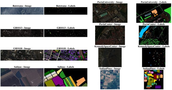
Figure 1.
False color composite images and corresponding label maps for each dataset used in our empirical evaluation. For each dataset, the left panel shows a false color composite generated from the hyperspectral data, and the right panel shows the ground truth labels, where each non-black color represents a distinct class and black pixels indicate unlabeled regions. Note: Images were resized to fit the layout; relative spatial dimensions across datasets are not preserved.
The selected datasets span a broad range of relevant properties: they include both relatively small and large imagery, datasets with few and many classes, and a wide range of labeled pixel densities. These characteristics critically influence the feasibility of unbiased sampling. Larger datasets provide more space to separate training and testing patches. A higher proportion of labeled pixels increases the number of valid CPLs, which expands the number of possible training and testing samples that satisfy separation constraints. Finally, datasets with fewer classes reduce the likelihood that stratification or commensurate class distribution requirements will constrain spatial assignment.
Provided that these datasets are commonly utilized, they appear and are discussed in detail in numerous other research articles. Given this and the fact that this work is more concerned with appropriately sampling remotely sensed imagery to develop machine learning models, and not necessarily developing a machine learning model, we only discuss the datasets to provide the proper credit and context. Due to the age and long-standing use of these datasets, it was challenging to trace their original sources. The only exception is GRSS18, which was retrieved from its original source, the IEEE 2018 Data Fusion Contest website [19]. GRSS13 was retrieved from Figshare [21]. The rest of the datasets were retrieved from the University of the Basque Country Computational Intelligence Group (GIC) Hyperspectral Remote Sensing Scenes website [20]. The GIC website provided data with commonly used preprocessing steps applied (such as dropping noisy spectral bands).
GRSS18 and GRSS13 were originally provided to the participants of the IEEE Geoscience and Remote Sensing Society (GRSS) Data Fusion Contests in the years of 2018 [22] and 2013 [23] respectively. Both datasets were acquired by the National Center for Airborne Laser Mapping (NCALM) in February of 2017 and June of 2012. GRSS18 provides three co-registered data modalities (hyperspectral, multispectral lidar, and high-resolution RGB). GRSS13 provides two co-registered modalities (hyperspectral and lidar). Both provide corresponding semantic pixel labels. Each depicts approximately 5 km2 of the University of Houston campus and its surrounding areas.
Pavia Center and Pavia University were acquired under the HySens project managed by the German Aerospace Center (DLR) and sponsored by the European Space Agency (ESA) [24]. Both datasets were collected during a single flight over Pavia, Italy, in July 2002 using the ROSIS-03 sensor [25]. Each provides single modal hyperspectral data with corresponding semantic pixel labels. The Pavia Center depicts the city center of Pavia and the river Ticino that runs through it. Pavia University depicts the Engineering School at the University of Pavia.
Botswana and Kennedy Space Center both provide single modal hyperspectral data and corresponding semantic pixel labels. Botswana was acquired by the National Aeronautics and Space Administration (NASA) Earth Observing-1 (EO-1) Hyperion sensor between 2001 and 2004 [26]. It depicts the Okavango Delta, Botswana. The Kennedy Space Center was acquired by the NASA Airborne Visible/Infrared Imaging Spectrometer (AVIRIS) sensor in 1996 [27]. It depicts the Kennedy Space Center in Florida, USA, its labels were derived from the Landsat Thematic Mapper (TM).
Indian Pines and Salinas were captured using the AVIRIS sensor and both provide single modal hyperspectral data and semantic pixel labels [28]. Indian Pines depicts farmland in the Northwestern portion of Indiana, USA. Salinas also depicts farmland but from the Salinas Valley in California, USA. These two datasets represent two of the overwhelming most studied small hyperspectral remote sensing datasets based on our survey results.
2.4. Survey Procedures
The primary objective of this survey is to address gaps identified in the existing literature; no previous survey of the field’s literature covered more than 20 research studies. The most comprehensive survey to date, conducted by Nalepa et al. [9], reviewed 17 works. Consequently, our survey aimed to achieve the following secondary objectives: (1) identifying the breadth of sampling methodologies implemented in remote sensing, (2) assessing how correlation is recognized and mitigated in practice, (3) compiling representative small or single-image datasets used in practice, and (4) evaluating the reproducibility of sampling algorithm implementations within the field. The survey was conducted in the following three main stages: (1) article search, (2) article review, and (3) article analysis. A flowchart of this process is provided in the Appendix A, Figure A1.
- Article search: The search for relevant articles was performed using Google Scholar [29] and Dimensions.ai [30], which together have indexed over 200 million articles [31]. The search began in December of 2023 and ended in March 2024. Various search terms were employed, including combinations of the following:
- Contexts: remote sensing, single image, small dataset, etc.
- Datasets: Indian Pines, Salinas, Pavia, Trento, GRSS, Trento, etc.
- Modalities: Hyperspectral, Multispectral, SAR, LIDAR, etc.
- Keywords: sampling, algorithm, methodology, i.i.d., etc.
The search results were reviewed in descending order of relevance. Each search result was assessed until it was determined to be irrelevant to the context of this study. A secondary search was also conducted by examining the references cited within the selected articles to identify additional key works. - Article review: The review process was designed to ensure that each article selected for the survey was thoroughly evaluated for its relevance and contribution to the study objectives. This multi-pass review process aimed to filter out irrelevant works efficiently while retaining those that provided useful insights.
- First pass: Titles and abstracts were reviewed to ensure general relevance to the study context. This initial screening aimed to quickly eliminate articles that were clearly outside the scope of remote sensing and/or machine learning.
- Second pass: The article text was skimmed to verify the development of a machine learning model. During this stage, we focused on identifying whether the articles involved empirical studies that implemented sampling methodologies, as well as the specific characteristics and sizes of the datasets used.
- Third pass: A full read-through was conducted to confirm the article’s relevance to this study’s objectives. This comprehensive review included a detailed examination of the methodologies, results, and discussions to ensure that the articles provided substantive insights into the research questions.
Articles were included in the final analysis if they met all of the following criteria: (1) The study involved supervised machine learning using remotely sensed imagery, (2) training and testing data were created using a spatially defined sampling procedure, and (3) at least one empirical experiment was conducted. Articles were excluded if they failed to meet any of the inclusion criteria or if spatial sampling was not required due to the dataset design. For example, when datasets consisted of many independent small images that could be directly ingested by the model without the need to spatially partition a larger image. These criteria were applied consistently throughout all three passes of the review process. - Article analysis: Following the review process, selected articles underwent detailed analysis to extract and categorize relevant attributes. The goal was to synthesize this information to provide a comprehensive understanding of current practices and highlight areas for improvement within the field. The attributes were:
- Year: The year that the article was published.
- Datasets: Identification of the dataset(s) used in each article. This compilation serves as a resource for researchers seeking representative datasets for their own experiments and to explore the characteristics of such datasets. The categories for this attribute were identified based on each unique dataset encountered during the survey.
- Sampling method: Identification of sampling methodology used. Each technique was analyzed against the desirable characteristics outlined in Section 2.1, as well as its application in different scenarios. The categories for this attribute were identified based on each unique sampling methodology encountered during the survey.
- Sampling documentation: Assessment of the reproducibility of sampling algorithms based on provided implementation details. This involved evaluating whether the articles provided sufficient information to replicate their sampling methodologies, including algorithm descriptions, code availability, and parameter settings. The categories for this attribute were . Articles categorized as “Full” contained complete pseudo-code or algorithm implementation along with parameter settings to fully reproduce the sampling method. “Partial” articles were lacking sufficient detail to completely reproduce the sampling method or results, but enough that informed research could create similar results. “None” articles did not contain enough detail, or any detail, on the sampling method used.
- Overlap correlation issues: Evaluation of whether the chosen sampling methodologies had issues with overlap correlation; this attribute does not address spatial autocorrelation (all sampling methodologies will technically have some non-zero amount of spatial autocorrelation due to patches being drawn from the same contiguous dataset image). The categories for this attribute were . Articles categorized as “Yes” used a sampling method that had verifiable issues with overlap correlation (such as random sampling). “No” articles used a sampling method that has no issues with overlap correlation, that is, they maintained a P minimum distance between training and testing samples. “Unknown” articles were ambiguous in their documentation making it difficult to fairly state if they did or did not allow overlap correlation.
- Correlation issue acknowledgment: Evaluation of studies to determine if they recognized the potential issue of correlation, both overlap correlation and autocorrelation, between training and testing dataset. This attribute does not assess whether the issue was present nor mitigated, only if the authors recognized that correlation was an issue. The categories for this attribute were , articles either directly stated that there was some issue with the correlation between training and testing sets or not.
Some of the categories used in the article analysis are inherently subjective, including Correlation Issue Acknowledgment and most notably Sampling Documentation. Although the best effort was made to ensure fairness and equity when assigning these attributes to articles, it is important to acknowledge that bias may still be present. The categorization was based on the authors’ interpretations and assessments, and while these were conducted as objectively as possible, variations in judgment can occur. Nonetheless, these subjective categories offer insight into current practices and highlight areas where further clarity and standardization could be beneficial.
3. Results
This section presents the findings of the study. It begins with an overview of the survey results, highlighting the number of unique sampling algorithms identified and their methods of correlation mitigation, if any. Each unique sampling method is then described in detail. A new sampling algorithm, clustered partitioning, is introduced, offering an automated approach to partitioning-type sampling. The identification of a Python library containing all the identified sampling methods is also discussed. Finally, the results of the empirical testing are presented, assessing the desirable characteristics of the sampling methods and evaluating their effectiveness.
3.1. Survey Results
This survey yielded 146 articles. These articles were published between 2015 and 2023 which reflects a natural concentration of research due to two key factors. First, the GRSS13 and GRSS18 data fusion contests introduced multimodal hyperspectral and lidar datasets that sparked significant interest in the field, providing larger, more diverse datasets for research. Over half (55%) of the articles were directly motivated by these datasets. Second, it was not until the 2010s that advancements [32] in general-purpose GPU (GPGPU) computing made CNNs computationally feasible on a large scale, reigniting interest in computer vision [33,34] and enabling more complex analyses of remote sensing data. The distribution of articles by publication year is shown in Figure 2; Table A1 in the Appendix B provides a detailed reference for each article by year.
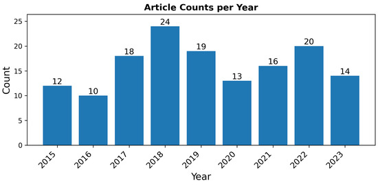
Figure 2.
Distribution of surveyed articles by publication year.
The survey encompassed 68 unique datasets, with the most frequently used being Pavia University (66 uses), Indian Pines (57), GRSS13 (49), and both GRSS18 and Salinas (32 each). Associated article counts are detailed in the Appendix B, Table A7 and Table A8. Many datasets are multimodal, containing diverse data types including hyperspectral imagery and 3D lidar. While hyperspectral data are most common, the presence of co-registered multimodal data suggests that correlation issues can arise across both image- and non-image-based modalities.
Several large datasets were identified in the survey, some exceeding the size of GRSS18 by orders of magnitude. For instance, Alhassan et al. [35] used the GeoManitoba dataset (13,777 × 16,004 pixels), generating 17,000 patches from overlapping grid windows. However, they did not specify how patches were assigned to train and test sets, leaving open the possibility of overlap correlation despite the dataset’s size. Similarly, Filho et al. [36] worked with the Cerrado dataset comprising 55 large, overlapping images and noted that overlapping areas were excluded from test images to prevent contamination—highlighting the importance of spatial structure even in large datasets.
3.1.1. Issue Acknowledgments
Figure 3 displays the distribution of articles by acknowledgment of correlation issues, with detailed article references per method provided in the Appendix B, Table A5. A significant concern highlighted by this survey is that over 90% of the articles do not acknowledge the potential for correlation issues. This oversight is particularly troubling given the frequent application of random sampling and the subtle nature of correlations in remote sensing data, which often remain undetected unless specifically investigated. The lack of recognition of these correlation issues is not entirely surprising due to the intricate dynamics involved. It can be likened to a “chicken or the egg” conundrum—until a sufficient number of articles that handle practical applications acknowledge and address correlation issues, the topic may not receive the emphasis needed to ensure it is routinely considered. This situation results in a cycle where the importance of understanding and mitigating correlation is under-discussed and, consequently, often overlooked in the initial stages of model development.
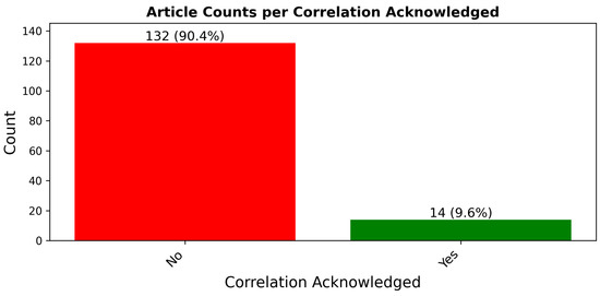
Figure 3.
Distribution of articles based on their acknowledgment of correlation, showcasing the large percentage of articles not recognizing the pitfalls of correlation.
The trend of acknowledging correlation issues over time, as illustrated in Figure 4, shows weak to moderate evidence of increasing recognition. Acknowledgment starts with approximately 10% of articles in 2015–2016 up to 20% in 2023. However, despite this gradual improvement, the data reveals that the issue is still not receiving sufficient attention to position it at the forefront of considerations during the practical development of machine learning models. The slow shift suggests a growing awareness, yet it emphasizes the need for a more pronounced and systematic approach to integrating considerations of correlation mitigation into the sampling methodologies employed across the field. This change is essential to advance the fair assessment of machine learning models, ensuring that comparisons of model generalizability across the domain are consistent.
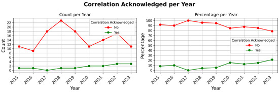
Figure 4.
Annual trends in acknowledging correlation in surveyed articles, shown as counts and percentages per year.
3.1.2. Overlap Correlation Issues
Figure 5 displays the distribution of articles by the presence of overlap correlation issues, with detailed article references per correlation existence or not provided in the Appendix B, Table A4. This figure shows that 48% of the surveyed articles used a sampling method, which induced an overlap correlation between training and testing data. Moreover, 18% of the articles were categorized as not having an issue with overlap correlation, and the final 34% were marked as possibly having an issue with overlap correlation. The usage of the Unknown category was necessary due to the considerable amount of missing or partial documentation of sampling methods used in the collected articles.
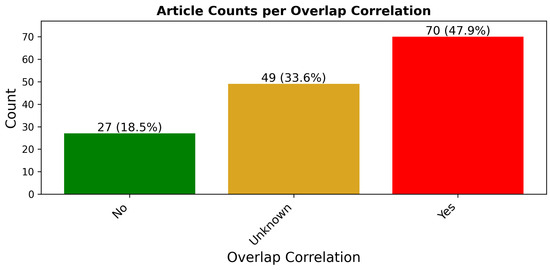
Figure 5.
Distribution of articles based on their sampling method’s potential to induce correlation. We argue that the majority of ‘Unknown’ articles are realistically ‘Yes’ articles. Following this, this highlights that the majority of surveyed articles have issues with overlap correlation.
Similar to the trend of acknowledging correlation issues over time, there is also a slight improvement in the percentage of articles without overlap correlation issues, as shown in Figure 6. Over the years, the percentage of articles identified as having no overlap correlation issues has slightly increased, which could imply a growing awareness and mitigation of such issues. However, despite this modest improvement, the prevalence of correlation problems remains significant, underscoring the need for more consistent attention and deliberate strategies for addressing these issues.
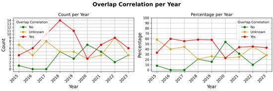
Figure 6.
Annual trends of overlap correlation presence in surveyed articles, shown as counts and percentages per year.
3.1.3. Issue Acknowledgment and Overlap Correlation Issues
When inspecting the intersection of the attributes acknowledgment of correlation (AC) and overlap correlation (OC), an interesting subset of articles appears. Figure 7 and Table A6 in the Appendix B provide a comprehensive breakdown of all possible combinations of these combined attributes with the above-mentioned table in the Appendix B providing further details on each article reference in relation to the specific attribute intersection.
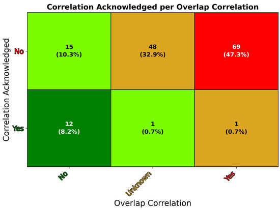
Figure 7.
Heatmap showing the intersection of two attributes: acknowledgment of correlation issues (AC) and overlap correlation presence (OC) in the reviewed articles. The heatmap categorizes the results into six possible combinations of these attributes. Green cells indicate desirable or permissible outcomes where correlation issues are either acknowledged or avoided (AC-Yes OC-No, AC-Yes OC-Unknown, and AC-No OC-No). Yellow cells represent articles with unknown or concerning overlap correlation statuses (AC-Yes, OC-Yes, and AC-No, OC-Unknown). Red cells highlight undesirable outcomes, where correlation is unacknowledged, and overlap correlation is present (AC-No, OC-Yes).
The intersection of these attributes reveals that 80% of articles do not acknowledge correlation issues, and either possibly (33%) or definitely (47%) employ sampling methods that induce overlap correlation. This finding aligns with the concerns expressed in the previous sections—that correlation issues are frequently neither acknowledged nor addressed in the field of remote sensing. Among the articles, there are notable exceptions to this trend. Twelve articles acknowledge correlation issues and have no overlap correlation issues (AC-Yes, OC-No). Fifteen articles neither acknowledge correlation issues nor have overlap correlation issues (AC-No, OC-No). Additionally, one article [37] acknowledges correlation and might have overlap correlation issues (AC-Yes, OC-Unknown), while another [38] both acknowledges correlation issues and has overlap correlation (AC-Yes, OC-Yes).
Among the 12 articles that acknowledge correlation issues without overlap correlation issues, five utilized partitioning-type sampling methods—Bigdeli et al. [39], Filho et al. [36], Guiotte et al. [40,41], and Zhang et al. [42]. Gbodjo et al. [43] employed simple random sampling but enforced a minimum distance of P between training and testing samples to avoid overlap. Hong et al. [44] classified only single spectra, which avoids overlap correlation but not necessarily spatial autocorrelation. Zhu et al. [45] used grid-type sampling and confirmed the absence of overlap between training and testing sets. The remaining articles by Acquarelli et al. [46], Liu et al. [27], Zhang et al. [47], and Zou et al. [48] introduced four distinct sampling algorithms identified in this survey.
Of the 15 articles that neither acknowledged correlation issues nor exhibited overlap correlation, 12 employed partitioning-type sampling methods [49,50,51,52,53,54,55,56,57,58,59,60]. Additionally, Li et al. [61] and Sun et al. [62] utilized grid-type sampling with strategically spaced grids (i.e., the CPL grid is spaced at the patch size P) to avoid overlap. Hong et al. [63] classified single spectra, avoiding overlap correlation. We specifically do not penalize these articles for not acknowledging correlation issues directly, as it is acceptable not to raise such concerns when none is verifiably present.
Collectively, the 27 articles mentioned encompass all 17 surveyed articles that utilized partitioning-type sampling methods, as well as more than half of the 8 articles that employed grid-type sampling (Refs. [35,64,65] are the remaining articles that used Grid Sampling, although they lacked adequate documentation to confirm the absence of overlap correlation issues). The upcoming section will provide further details, but these 27 articles represent all identified instances where sampling methodologies were successfully employed that fully mitigated overlap correlation.
Fang et al. [37] acknowledged potential correlation issues and cited a cluster sampling strategy [10] to reduce overlap, although it is unclear whether overlap was fully eliminated. The original method [5] asserts non-overlapping regions, but no work in the citation chain provides implementation details, highlighting the need for more rigorous documentation of sampling procedures in remote sensing.
3.1.4. Sampling Documentation
Figure 8 displays the distribution of articles by the amount of sampling method documentation provided, with detailed article references per category provided in the Appendix B; see Table A3. Moreover, 87% of the articles surveyed provided only partial documentation regarding the sampling method used to generate training and testing data for model development. The partial category is defined as containing enough information for informed research to recreate similar results. While this level of documentation might have minimal impact outside of this field (using datasets that contain multiple non-contiguous images), it is imperative within the context of remote sensing that a complete understanding of the sampling methodology is important for accurate model assessment and comparability. This finding amplifies the issues of correlation and suggests an additional problem of scientific non-repeatability.
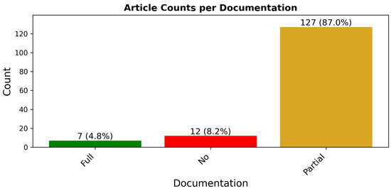
Figure 8.
Distribution of articles based on their level of sampling documentation.
While the 12 articles that provide no documentation are unremarkable, the 7 articles that offer full documentation form an interesting subset. Four of these articles [27,47,48,66] introduce unique sampling algorithms identified in this survey. The remaining three articles, while not introducing unique methods, are notable for different reasons. Paoletti et al. [67] and Zhu et al. [68] both employed simple random sampling methodologies, but what sets them apart is the depth of their documentation. Paoletti et al. used stratification to address class imbalance and provide detailed descriptions of the steps taken to create training and testing sets. They justified their thorough documentation by stating, “we could not identify a common pattern about sampling selection strategies in literature” [67]. To our knowledge, these two articles are the only ones in the survey that use simple random sampling and provide comprehensive documentation of its usage.
The third article, by Hong et al. [52], implemented a form of grid-type sampling that progressively shifts grid coordinates during training. The model’s task involved cross-modality learning, where—given both modalities during training—it predicts labels for the opposite modality using only one during testing. Hong et al. compared their grid approach against simple random sampling and found that their method resulted in approximately 20% higher overall accuracy. They attributed this improvement to the fact that “randomly selecting patches would los[e] the useful information to a great extent” [52]. Given the overlapping patches generated by their grid technique, this explanation seems valid. Grid-type sampling with overlap ensures coverage of the entire image, providing the model with more unique training observations, whereas random sampling does not guarantee such comprehensive coverage.
3.1.5. Unique Sampling Algorithms
Figure 9 shows the distribution of articles by sampler type, with detailed references for each category provided in the Appendix B; see Table A2. The sampler types identified in the figure are those discovered during the article survey. Our background literature review also identified many articles that were not application-based but, like this work, investigated and studied correlation issues of sampling methods. Furthermore, this work proposed a new sampling method. Table 3 lists all sampling methods identified during the survey and literature review.
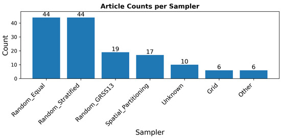
Figure 9.
Distribution of articles based on their sampling algorithm. In 10 of the surveyed articles, we could not identify the sampling method utilized (10 of 12 of the “No” sampling documentation articles). The 6 articles listed as “Other” were single-instance unique sampling methods that were compressed to make a more visually appealing figure. These are listed explicitly in Table 3.
Table 3.
All unique sampling methodologies identified during the article survey, literature review, and those developed in this work. Note, 10 articles with unknown sampling methods are not accounted for in the counts.
The criteria for the uniqueness of a sampling algorithm are difficult to define and somewhat subjective. It is also notably challenging to compare sampling methods when most surveyed works provide only partial documentation. While there are obvious and meaningful differences, irrelevant differences also exist. For example, Zhu et al. [68] introduced a method called “hierarchically balanced sampling”, which involves providing the entire dataset image (from a single image dataset) as input to the model during training. In each training iteration, a different subset of CPLs is used as the training set, determined in a stratified manner. This method is essentially what we call Random Stratified sampling, with the only difference being that in one case, the training CPLs used during each model iteration are pre-selected, while in the other, they are not.
Additionally, there are instances where data processing steps before or after sampling might be mistakenly considered part of the sampling methodology, thus falsely attributing uniqueness. For example, Liu et al. [69,70] used a method we call Random Equal sampling. After sampling, all labels for pixels not in the training set are changed to the unlabeled class’ value. Regardless of this action’s implications, we consider it a form of sample post-processing, not a unique sampling method. The effects of data processing steps before or after sampling can undoubtedly impact the correlation between training and testing sets (see the empirical study on mean filter pre-processing by Liang et al. [4]). However, this work only focuses on sampling methods and their effects on correlation, with further discussion on this topic provided in Section 4.
Lastly, we identified instances of methodological error in model development that we did not consider unique sampling methods. For instance, Yang et al. [71] used a form of random sampling to generate training data. However, regarding testing data, they noted, “we test the performance on the whole image” [71], which suggests that their performance reporting is conducted on both the training and testing portions of the image—a practice that can yield an overestimate of the true performance of the model. Another example, albeit unclear due to lack of documentation, is from Cuypers et al. [72]. They used the GRSS22 dataset, which contains 333 images; as noted, “we used 333 tiles out of which we extracted 500 training points per class” [72], suggesting a similar approach to Yang’s, where performance was reported on training data.
Table 3 categorizes each identified sampler into one of four types, namely, random, controlled, grid, and partitioning. All sampling methods identified naturally fall into these categories:
- Random: This category includes what has been previously described as random sampling, where CPLs are randomly selected and assigned based on some underlying distribution. Random sampling is commonly used outside the field of remote sensing with success, but as noted in the introduction, it is often inappropriate in this context.
- Controlled: Samplers in this category systematically select CPLs to address issues with spatial autocorrelation, attempting to ensure unbiased results. However, the issue of overlap correlation is sometimes not addressed directly.
- Grid: These samplers select CPLs based on a predefined grid of points overlaid on the image. Grid sampling is used to provide coverage of the entire spatial expanse and is sometimes closely related to the motivation for partitioning-based samplers.
- Partitioning: This category encompasses samplers that spatially partition the image into disjoint training and testing regions. Partitioning samplers are applied specifically to overcome overlap correlation.
The table also provides the original reference for each method, if available, along with the original name of each method. In this work, we assign distinct names to each sampling method identified to address conflicting naming conventions from the original sources. What follows in a succinct description of each method; Section 3.3 discusses more concrete software implementations in the Python 3 programming language of a majority of the identified methods.
3.1.6. Sampling Methods Preface
Before describing each sampling method, it is important to introduce a shared concept applicable to most sampling methods: determining the initial set of valid CPLs from the dataset. This set represents all pixel locations within the image at which patches may be localized, all other pixel locations are invalid. When discussing CPLs without reference to a specific set (e.g., “training CPLs”), this is what is being referenced. We propose two general approaches for identifying these CPLs. The first approach involves using every labeled pixel as a potential CPL. This method is straightforward, but it presents challenges for CPLs that are less than of the edge of the image. In such cases, the resulting patch may be smaller than the desired size or require padding to meet the required dimensions. This approach demands additional consideration to understand the implications of such padding or incomplete patches.
In this work, we adopt the second approach. This approach uses only labeled positions that are at least distance from the edge of the dataset’s image(s). This ensures that only patches of the desired size are created, eliminating the need for padding and providing a consistent basis. Interestingly, none of the identified works explicitly mention this concept. However, given the lack of discussion in survey articles about padding samples, it seems likely that the second approach is more commonly used. If the first approach is more prevalent, this represents another example of inadequate documentation in the field.
Another concept that is important to introduce and, moreover, reinforce, prior to discussing the sampling methods, is the relationship between CPLs and patches. As previously discussed, a CPL defines the pixel location that localizes a patch. As a result, there is a near equivalence of CPLs and patches. In the following sections, we sometimes use this interchangeably, notably in the Grid Sampling Methods section. It is sometimes useful to refer to CPLs and other times the patches that are a result of slicing a sized region around a CPL. Most algorithms deal solely with CPLs and the instantiation of patches via slicing is post facto. Some algorithms assign patches to the training or testing set based on the content of patches, thus, these algorithms perform slicing in situ to attain this ability.
Given the generally partially documented nature of most sampling methods identified in the literature, the descriptions of unique sampling methods we offer here contain several assumptions about the authors’ intentions. Some of these assumptions are based on logical approaches that a competent researcher might use to achieve the stated mechanisms, while others are inferred from the context provided in the original articles. To ensure transparency, we include original quotes from the source articles alongside our descriptions when applicable. This not only highlights the level of documentation provided in the original works but also clarifies how we have interpreted and expanded upon these descriptions to form our assumptions. By doing so, we aim to bridge the gaps in documentation and provide a more comprehensive understanding of each sampling method.
3.1.7. Sampler Footprint Plot
In this section, we introduce the concept of a “footprint plot”, which we will utilize extensively in the following sections to quickly visualize and understand the outcomes of sampling methods. Specifically, the footprint plot helps to visualize the status of each pixel location (which we will refer to simply as “pixel” in this section for brevity) after the sampling process is complete. The status of a pixel refers to whether it is part of the training or testing set, whether it is within a patch or selected as a CPL, and whether it is valid (non-overlapping) or invalid (overlapping). The following enumeration provides all possible statuses and their corresponding colors, with a pictorial example of their meanings shown in Figure 10.
 Unused pixel: A pixel that is unused during model development. It may be labeled or unlabeled.
 Overlapping patch: A pixel that is not a CPL. It is a member of both a training and testing patch (i.e., overlap correlation).
 Training patch valid: A pixel that is not a CPL. It is a member of a training patch and not a member of any testing patch (the patch it belongs to may or may not overlap in other location(s)).
 Testing patch valid: A pixel that is not a CPL. It is a member of a testing patch and not a member of any training patch (the patch it belongs to may or may not overlap in other location(s)).
 Training CPL valid: A pixel that is a training CPL. All pixels in its resulting patch do not overlap any other pixels that fall within the testing set.
 Training CPL invalid: A pixel that is a training CPL. At least one pixel in its resulting patch falls within the testing set (i.e., causes overlap correlation).
 Testing CPL valid: A pixel that is a testing CPL. All pixels in its resulting patch do not overlap any other pixels that fall within the training set.
 Testing CPL invalid: A pixel that is a testing CPL. At least one pixel in its resulting patch falls within the training set (i.e., causes overlap correlation).
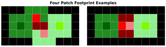
Figure 10.
Two examples of four patch “footprints” with pixel coloring referring to pixel status. In both examples, two training patches and two testing patches are shown. The training and testing patches on the horizontal outer edges of the image have no inter-set overlap (i.e., training–testing) but both have intra-set overlap (i.e., training–training). As a result, both of these CPLs (■,■) and all pixels (■,■) in the resulting patches are deemed valid. The training and testing patches on the inside of the images overlap each other. As a result, both of these CPLs (■,■) are deemed invalid because a subset of pixels in their resulting patches overlap (■), while the other subset is deemed valid (■,■).
An important aspect to understand about these statuses is that any given pixel can possess multiple statuses simultaneously. For example, in the right-hand example of Figure 10, a training and testing CPL are Rook neighbors. The invalid training CPL (indicated in ■) is directly adjacent to an invalid testing CPL (indicated in ■). This proximity means that both the invalid training and testing CPLs also share the overlapping patch status. To manage this status overlap, we prioritize the statuses in the order stated in the enumeration above when generating (coloring) footprint plots.
A limitation of this prioritization scheme, and footprint plots in general, is that they cannot detect or visually represent scenarios where a single CPL produces multiple patches, nor can they show the assignment of those patches. In other words, if a sampling method were to select the exact same CPL twice, resulting in a duplicated patch (regardless of whether the duplicated patches are assigned to the training or testing sets) this would not be reflected in the footprint plot. However, our review of the sampling methods revealed that none of the methods we examined exhibited this behavior.
Figure 11 provides an example footprint plot of a small 32 × 32 section from the top center region of the Indian Pines dataset, using the output of the Liang Controlled sampling method with and . This figure is useful not only for understanding the pixel statuses and the associated coloring scheme but also for illustrating how footprint plots can visually assess the output of a sampling method, particularly in terms of spatial autocorrelation and overlap correlation.
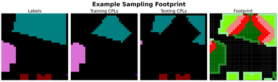
Figure 11.
Example of a footprint plot using a small 32 × 32 section from the top center region of the Indian Pines dataset produced by the Liang Controlled sampling method with and . The first panel shows the dataset pixel labels, where each non-black color represents a distinct class and black pixels indicate unlabeled regions. The second and third panels show the subset of labels selected as training and testing CPLs, respectively. The final panel displays the same spatial region colored using the enumeration of pixel status, illustrating the footprint resulting from the selected training and testing CPLs.
In the figure, one can quickly gauge the extent of overlap correlation by comparing the relative amount of green-colored pixels (■,■,■,■) to the red-colored pixels (■,■,■). Additionally, it is possible to make a general assessment of the potential for spatial autocorrelation by observing the clustering and distribution of dark green-colored training set pixels (■,■) in relation to light green-colored testing set pixels (■,■), regardless of their specific shades. Furthermore, footprint plots provide insight into the overall total dataset coverage of all patches, as well as the relative coverage between training and testing patches, which are related to the desirable sampling characteristic of Bernoulli distribution allocation.
We present the footprint plot as a contribution of this work, offering a concise and efficient way to convey qualitative information about how datasets were sampled. Given our survey results, which highlight the low number of articles that fully document their sampling methods, along with the challenges of publishing exact sampling outputs, the footprint plot offers a potentially easier and more accessible way to share this information. Currently, there is no standard method across the field for presenting sampling details. We suggest that footprint plots could become part of a potential standard for reporting this information.
3.1.8. Random Sampling Methods
All random sampling algorithms operate by identifying and randomly sampling from a probability distribution to form the training CPL set. Once the training set is created, all unselected CPLs are assigned to the testing set. Each type of algorithm utilizes a distinct probability distribution for selecting CPLs, motivated by different desirable characteristics.
Random Equal sampling uses a truncated uniform probability distribution across all class labels in the original dataset, with the truncation threshold set by the minimum count per class. This ensures balanced class representation. The Random Stratified sampling method selects CPLs according to the empirical distribution of class labels in the original dataset, thereby preserving the natural class proportions (Figure 12). Random Uniform employs a uniform probability distribution across all pixel locations, treating each pixel equally without regard to class membership. Random GRSS13 is a static variant of Random Stratified. Its training and testing sets were pre-determined by the organizers of the IEEE GRSS 2013 Data Fusion Contest and are provided as the recommended sets for model development.
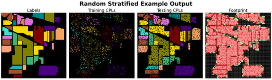
Figure 12.
Example execution of the Random Stratified sampling algorithm on the Indian Pines dataset with and . In the footprint plot, it is apparent from the large number of red-colored pixel locations that even with a small patch size and low amount of training data a large amount of overlap correlation is present. However, Random Stratified and most other random-type samplers can achieve nearly perfect commensurate class distribution and the desired .
Clark Stratified [66] (Figure 13) starts with the same distribution used in Random Stratified but modifies it by logarithmically weighting classes to enhance the representation of under-represented classes. This method calculates the number of training CPLs per class by taking the logarithm of the “class area” [66] (assumed to be the count of pixels in the original dataset with a given class label) and dividing it by the sum of the logarithms of all class areas. This fraction is then multiplied by the total number of desired training CPLs (i.e., times the total number of pixels in the dataset), rounding up to ensure non-zero class representation for small area classes.
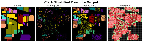
Figure 13.
Example execution of the Clark Stratified [66] sampling algorithm on the Indian Pines dataset with and . When compared to the Random Stratified execution example in Figure 12 it is apparent that larger spatial area classes were sampled less frequently (olive-colored class) as expected. Regardless, a large amount of overlap correlation still exists.
The Liu Random [27] (Figure 14) sampling method, although fully documented, appears to misinterpret the approach introduced by Liang et al. [4] (Liang Controlled). Liu describes their sampling method as follows (quoted reference updated to match this work’s bibliography):
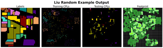
Figure 14.
Example execution of the Liu Random [27] sampling algorithm on the Indian Pines dataset with and . Compared to Random Stratified and Clark Stratified, and all other random-type sampling algorithms, the enforcement of a minimum P distance between CPLs results in no overlap correlation. However, this comes at the cost of considerably fewer patches being generated overall.
“we randomly chose one pixel belonging to one class as the central pixel and obtained training samples by region extension [4]. We chose 8 × 8 images by a region extended from one pixel to 8 × 8 images for unbiased datasets and obtained 8x8 images by a region extended for the training set. The 8 × 8 image-by-region extension involves finding one pixel as the central point and selecting the surrounding pixels to form the training sample” [27].
We interpret this as simply defining the desired patch size of their sampling method as and describing the process of extracting an patch from the dataset. This seems to be a misunderstanding based on Liang’s description: “the training samples are generated by extending a region from the seed pixel” [4]. A closer examination of Algorithm 1 and the corresponding text in Liang’s work reveals that “region extension” refers to growing a contiguous region of CPLs from a starting pixel location, not expanding a region of pixels into a single patch from a CPL. Liu Random is considered a unique sampling method because it explicitly states that overlapping patches are not created. Given this information and the fact that they use 200 patches for training, we understand Liu Random to be equivalent to Random Uniform with a P minimum distance between CPLs in the training and testing sets.
3.1.9. Controlled Sampling Methods
All controlled sampling algorithms operate by systematically selecting CPLs to address the issue of spatial autocorrelation, with various methods used to mitigate overlap correlation. Spatial autocorrelation is typically reduced by clustering CPLs into spatial groupings from which training or testing CPLs are selected, or by selecting CPLs in a way that naturally forms clusters. By creating global clusters, these methods induce high global spatial autocorrelation of the resulting patches, thereby reducing local spatial autocorrelation of pixel values, which can bias empirical error (as discussed in Section 2.1).
Zhou Controlled [3] (Figure 15) provides limited details on the implementation of their approach, stating only that they
“[...] sample continuously from a local area for each class. The randomness can be guaranteed by choosing different local areas across the data. Although this approach cannot completely eliminate overlap, the influence of testing data on the training step can be greatly reduced” [3].
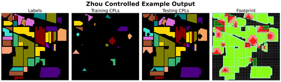
Figure 15.
Example execution of the Zhou Controlled [3] sampling algorithm on the Indian Pines dataset with and . Unlike random-type samplers, which do not enforce a minimum distance, the systematic selection of CPLs by controlled-type samplers results in low overlap correlation even without minimum P distance enforcement. A drawback of the Zhou Controlled method is that a single seed pixel, per class, is selected as the cluster center. If a small class partition is selected, when using rook neighbors to define “local area” [3], training CPL selection could end before the defined threshold is met. For example, the olive-colored class (soybean min-till in Indian Pines) unfortunately has the cluster center selected from its smallest partition, which is located almost exactly at the center of the image). As a result, only 33 training CPLs are selected instead of the 361 required to form the empirical distribution (with ).
We interpret this to mean that, for each class, a single CPL is randomly selected as a cluster center from the initial valid set. CPLs in the vicinity (we use Rook neighbors to define vicinity) are then sampled until a threshold (we use times total count per class to match the empirical distribution) is met. The selected CPLs are then assigned to the training set, and all other unselected CPLs for the class are assigned to the testing set. Notably, this method does not enforce a minimum P distance to prevent overlap correlation during sampling.
Liang Controlled [4] (Figure 16) provides a detailed pseudo-code of their sampling methodology in Algorithm 1 of their original work. This method begins by calculating all partitions (contiguous regions defined by Rook neighbors) of labels in the original dataset. Within each partition, a CPL is randomly selected as the seed location. From this seed, a region is grown by selecting neighboring CPLs until a specified count is reached, presumably in a breadth-first manner. The count is determined by multiplying by the total number of pixel locations in the partition. The selected CPLs across all partitions form the training set, while all remaining valid CPLs are placed into the testing set. This approach is extremely similar to Zhou Controlled, only differing in the number and location of cluster centers (seed pixels) selected per class. Furthermore, like Zhou’s method, this approach does not enforce a minimum P distance to prevent overlap correlation.
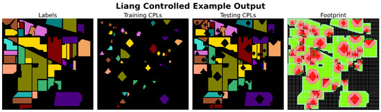
Figure 16.
Example execution of the Liang Controlled [4] sampling algorithm on the Indian Pines dataset with and . Liang Controlled is nearly identical in its approach to Zhou Controlled, the only difference being that it selects cluster centers from all partitions for each class. As a result, it does not fall prey to the issue discussed in Figure 15. However, this alteration has resulted in a large amount of overlap correlation compared to Zhou Controlled.
Hansch Controlled [5] (Figure 17) provides minimal implementation details, describing their approach as follows:
“[f]or each class the spatial coordinates of all samples are clustered into two clusters. Training samples of a class are randomly drawn from one of the clusters, the other cluster is used as test data. If two adjacent clusters (of any classes) contribute to train and test data, a spatial border around the corresponding training samples ensures non-overlapping train and test areas.” [5].
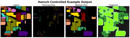
Figure 17.
Example execution of the Hansch Controlled [5] sampling algorithm on the Indian Pines dataset with and . The 2-clustering approach of Hansch Controlled results in training and testing patches that are maximally spatially separated “ensuring maximal independence between testing and training” [5] to greatly reduce possible spatial autocorrelation. Furthermore, the P boundary results in no overlap correlation. However, to achieve the desired Hansch Controlled could only select a subset of the CPLs from each class cluster assigned for training CPL selection. As a result, a large number of unselected training CPLs are unused during model development.
We infer that this involves clustering valid CPLs using a method such as K-Means with a parameterized number of clusters set to 2. For each class, the two clusters are then assigned as potential CPL sets for either training or testing. After selecting a specified count of training CPLs—likely in a stratified manner by multiplying by the number of pixels per class—a P boundary is placed around each training CPL to invalidate any CPLs in the testing clusters within this boundary. The remaining valid CPLs in the testing clusters are then added to the testing set.
Lange Controlled [6] (Figure 18) provides limited details on the implementation of their approach, describing it as follows:
“extracting larger contiguous regions using the class labels [...] and then distributing these disjointly between the training and test set [...] extraction of the contiguous regions is achieved with the DBSCAN clustering algorithm [...] This requires to establish a metric that evaluates said variety. The first two, [...] are the region area size and statistical variance. Based on this, sorting the regions in ascending, respectively descending order, and assigning them to the training set, up until the selected split percentage” [6].
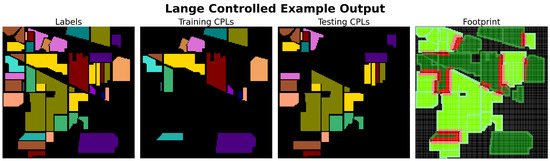
Figure 18.
Example execution of the Lange Controlled [6] sampling algorithm on the Indian Pines dataset with , , and cluster ordering by average variance across bands. By selecting entire partitions to add to the training set, large contiguous regions of CPLs can be created which reduces overlap correlation when a P boundary is not used. However, this assignment of CPLs to the training set results in non-commensurate class distributions and difficulty in achieving the desired .
We interpret this to mean that the valid CPLs for each class are clustered using DBSCAN to identify all label partitions. Each partition is then evaluated by calculating either its area or variance. Since there is no standard way to measure the variance of a multi-band image, we suggest using the average variance across bands. Once these values are calculated, the regions are sorted, regardless of class, and assigned to the training set. The assignment continues until the training set contains times the total number of initial valid CPLs. Notably, this method does not enforce a minimum P distance, which allows overlap correlation to occur during sampling.
Acquarelli Controlled [46] (Figure 19) provides the least information on their method, stating that they “propose to randomly select a single patch of pixels for each class to use as training data. We use a patch of 7 × 7 labeled pixels for each class as a training set, which ensures that we have enough training pixels (at most 49) per class” [46]. Although they suggest a patch size of , we allow flexibility for any desired patch size. While not explicitly stated, other parts of their work imply an understanding of overlap correlation issues. Therefore, to define the testing set, all CPLs within a P distance from the selected training CPLs are invalidated, and the remaining valid CPLs are used for the testing set.
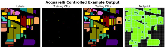
Figure 19.
Example execution of the Acquarelli Controlled [46] sampling algorithm on the Indian Pines dataset with and . The selection of a single training CPL per class and a P boundary results in extremely low spatial autocorrelation and no overlap correlation. However, this also results in a dearth of training observations for model development.
3.1.10. Grid Sampling Methods
All grid sampling algorithms operate by defining a regular grid that spans the extent of the original dataset image(s). Unlike other sampling types, the initial valid set of CPLs is defined by the pixel locations at the center of each grid cell (or, depending on convention, at the intersection points of grid lines). The grid can be either unstrided or strided. Unstrided approaches set the grid spacing equal to the desired patch size, resulting in no overlap between patches. Strided approaches, on the other hand, set the grid spacing to be less than the desired patch size, typically allowing for a overlap between patches. In strided approaches the same concerns described in Section 1.3 and Section 2.2.1 apply; as the patch size increases and the stride decreases, the likelihood of overlap correlation between training and testing patches grows significantly.
The Grid Simple (Figure 20) method uses CPLs as defined by the specified grid size, whether unstrided or strided. CPLs are then randomly assigned to the training or testing set with a probability of . A particular consideration for the Grid Simple method is dealing with patches that contain no labeled pixels. In remote sensing datasets, it is common for a large percentage of the image to be unlabeled. Consequently, grid sampling methods can generate a significant number of patches without any labeled pixels, which can pose challenges during model development. In our review of the literature, we did not encounter any work that effectively mitigated this issue for the Grid Simple method. The only solution we can propose is to remove these entirely unlabeled patches from the initial valid set before the assignment of the training or testing sets.
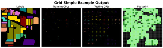
Figure 20.
Example execution of the Grid Simple sampling algorithm on the Indian Pines dataset with , , and an unstrided grid. Grid Simple sampling results in medium to low spatial autocorrelation due to the low count of total samples produced. Similarly, due to the unstrided nature of this example, no overlap correlation is present. However, this results in very few observations for model development. It also results in very few observations for model assessment, if only the CPL label is predicted during assessment as opposed to the entire testing patch. We discuss this tidbit further in Section 4.
Zhang Grid [47] (Figure 21) utilized an unstrided grid; the grid size is further required to ensure that each class is represented in at least two of the resulting patches. If the final grid size does not evenly divide the original dataset’s dimensions, padding is added to patches that do not meet the desired size. All CPLs that would result in entirely unlabeled patches are removed (Zhang et al. actually placed these into a “waiting for prediction” [47] set, which was unused during model development). Once the initial valid set of CPLs (and, thus, patches) is identified, the patches are assigned to the training and testing sets. The first step in this assignment is to place all patches containing only a single label type into the testing set (it is unclear whether these patches are allowed to contain unlabeled pixels). The remaining patches are then sorted by “category or by the number of samples within each category” [47]. The specific sorting algorithms are not well described, but an example of sorting by category is provided. To our understanding, the process involves iterating over each class, identifying all patches containing that class, and sorting them by the total number of matching labels in the patch. These patches are then split into the training and testing sets with a probability of . After the assignment, the patches are removed from the pool of unassigned patches, and the process continues until all patches are assigned to either the training or testing set.
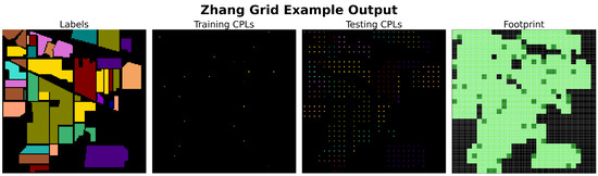
Figure 21.
Example execution of the Zhang Grid [47] sampling algorithm on the Indian Pines dataset with and . This presents a similar result to Grid Simple but with more label variation in the selected training patches. Due to the manner in which training and testing patches are assigned, it is difficult to achieve a desired or commensurate class distribution.
Zou Grid [48] (Figure 22) also employed an unstrided grid. Initially, all entirely unlabeled patches are discarded. Similar to Zhang Grid, all patches containing only a single label are placed into the test set (again, it is unclear if these patches may include unlabeled pixels). The remaining patches are then sorted in the order they appear when iterating through the grid by rows from top to bottom and columns from left to right, with the origin at the upper left-hand corner. After ordering, this set is divided into K subsets of equal size (with the final subset potentially being of unequal size). It is unclear how the value of K is determined; Zou et al. only noted the following: “The parameter K is limited by the percentage of pixels taken as training samples” [48]. In their work, they used . Finally, one of these K subsets is selected as the training set, one is set aside for validation, and the remaining subsets are added to the testing set. Notably, this is the only identified sampling method that explicitly provides a mechanism for generating a validation set, which we discuss further in Section 4.

Figure 22.
Example of the execution of the Zou Grid [48] sampling algorithm on the Indian Pines dataset with and . This presents a similar result to the Zhang Grid. Furthermore, he same drawbacks may be present, including difficulty in achieving a desired or commensurate class distribution. In the two specific examples presented for Zhang Grid and this Zou Grid result, the Zou Grid selected even fewer training CPLs.
3.1.11. Partitioning Sampling Methods
All partitioning sampling methods operated by defining at least two spatial partitions of the original dataset, from which CPLs were selected exclusively for either the training or testing set. The motivation behind this approach is its ability to readily ensure that no overlap correlation exists between the training and testing sets. Although often unstated in the literature, this method can also significantly reduce spatial autocorrelation when the number of spatial partitions is low, as only patches near the partition boundaries are likely to exhibit local spatial autocorrelation (we believe it to be a reasonable hypothesis that partitioning-based samplers could achieve the lowest possible spatial autocorrelation for a given dataset by identifying a partition boundary that maximizes the separation between labeled pixel locations, thereby minimizing the potential for local spatial autocorrelation near the boundary). However, a major drawback of this approach is the computational burden involved in identifying partitions that create commensurate class distributions. While we did not find any existing algorithmic solutions to this challenge in the literature, we propose one in our clustered partitioning sampling method, which will be discussed in the following section.
The Spatial Partitioning sampling method itself lacks a standardized algorithmic implementation. Four manual methods of identifying partitions appear in the literature. The first is the creation of two partitions from a single-image dataset [40,41,42,51,55,56,58,59] where one is selected for training and the other for testing. The second relies on the inherent partitioning of multi-image datasets [36,49,50,52,53,54] to create disjoint sets (this approach is essentially “random sampling”, as viewed from outside the field of remote sensing, on typical image-based datasets for classification). The third is the creation of multiple partitions from a single-image dataset [39], where some subset of partitions is used for training and the rest for testing (this technique approaches a form of random sampling with a P minimum distance between patches, as the number of partitions reaches a maximum). The final is the creation of two or more partitions per image in a multi-image dataset [57,60].
All of these identified methods accomplish the task of identifying spatially disjoint areas across the spatial extents of the entire dataset. Apart from the identified methods, many alterations can be made that still fit this precept. For example, in our previous work, Decker et al. [73,74], we utilized an alteration of the first method where instead of two partitions we created three. In this case, the third partition was used to create validation data for model development purposes.
3.2. New Sampling Method Implementation
In response to the lack of a standardized algorithmic implementation for spatial partitioning sampling methods identified during our literature survey, we introduce a new sampling method called clustered partitioning. Existing methods rely on manual or ad-hoc partitioning approaches that are often inconsistent and fail to fully address the challenges of creating commensurate class distributions while minimizing overlap and spatial autocorrelation. Clustered partitioning provides an automated solution by defining spatially disjoint partitions that ensure no overlap correlation, while also attempting to achieve the desired class balance and training-to-testing ratio. This method aims to fill the gap in current partitioning-based sampling techniques, offering a more structured approach to partitioning the spatial extents of remote sensing datasets.
Clustered Partitioning
Clustered partitioning is inspired by the Hansch Controlled [5] sampling method. The Hansch Controlled method creates two clusters for each class in the dataset, assigns one for training CPL selection and the other for testing CPL selection, and ensures a P boundary around the selected training samples. During the review of the Hansch sampling method, we realized that all labeled pixel coordinates could simply be spatially clustered to create two “global clusters” of CPLs; as opposed to the Hansch Controlled per-class method. These global clusters function similarly to the disjoint spatial partitions used by partitioning-type samplers.
Once these two global clusters are established, their centroids are calculated, and a perpendicular bisector is drawn, extending to the edges of the image. This bisection line then serves as the boundary between the two partitions. To prevent overlap correlation near this boundary, all CPLs within a tangential distance from the boundary are removed from the initial valid set. Finally, in an attempt to maintain the desired Bernoulli distribution allocation values , the partition with the fewest valid CPLs is assigned to the set type corresponding to .
Figure 23 illustrates an example output of the clustered partitioning sampling method on the Indian Pines dataset using and . This figure demonstrates that the automated approach of clustered partitioning generates a partition boundary that bisects the spatial extents of labeled pixels in the image. Notably, as a result of labeled pixels having static locations for a given dataset, the partition boundary that clustered partitioning creates is deterministic. The only change to the training and testing partitions will be how many CPLs near the boundary become invalid with larger patch sizes.
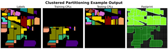
Figure 23.
Example execution of the clustered partitioning sampling algorithm on the Indian Pines dataset with and . Partitioning-based sampling methods, like clustered partitioning, result in extremely low spatial autocorrelation and no overlap correlation. However, this comes at the cost of great difficulty in achieving the desired or a commensurate class distribution similar to those found in grid-type sampling methods.
The primary limitation of clustered partitioning stems from the deterministic nature of its partition boundary. Once the boundary is established, the number and spatial distribution of valid CPLs on each side are fixed by the layout of labeled pixels in the dataset. As a result, both the achievable Bernoulli distribution allocation values and the resulting class distributions are not freely tunable, but are instead constrained by the geometry of the data. In the figure, it is apparent that much more than a amount of pixels were placed in the training set. One potential solution is to not include all CPLs from the training partition in the training set, similar to the method proposed by Hansch Controlled to address a related issue.
The second drawback is that—due to the static partition boundary—achieving commensurate class distribution is rare. For instance, in the example shown in Figure 23, the training partition lacks representation of 5 of 16 classes (class indices 4, 8, 12, 15, 16), while the testing set has no representation of 4 of 16 classes (class indices 1, 7, 9, 13). While a solution for including non-represented classes remains elusive, a potential approach to generating more commensurate class distributions is similar to achieving the desired values, that is, employing Random Stratified sampling of the subsets of CPLs within the training and testing partitions to enforce more balanced class distributions.
3.3. Sampling Algorithm Software Library
In addressing the common issue of partially and poorly documented sampling methods in the field, we have identified an existing software library that provides comprehensive implementations of various sampling methods. This library is particularly noteworthy because it fortuitously includes well-documented and concrete implementations in the Python programming language, making it a valuable resource for the research community. The software library can be accessed at https://github.com/kevindckr/samplify (accessed on 2 December 2024).
Given the incomplete documentation of most identified samplers in the literature, this software library necessarily assumes certain interpretations of the original intentions and implementations of these methods. These assumptions, along with any modifications made to align with contemporary practices, are thoroughly documented within the source code. This transparency ensures that users can fully understand the basis for the implemented methods and adjust them as needed for their specific applications. Additionally, the codebase includes tools to characterize each sampling method as described in this article, providing implementations for measuring the objective desirable characteristics of each sampler. The complete set of implemented sampling methods is listed in Table 4.
Table 4.
All sampling methodologies implemented in the provided software library.
3.4. Sampling Algorithm Empirical Testing
We used the identified software library to conduct 3024 sampling algorithm experiments. Each experiment varied four parameters: sampling algorithm, dataset, patch size, and . The values for these parameters are provided in Table 5. We recorded four measurements that represent the desirable characteristics, namely, overlap percentage (OP), Moran’s I (MI), KL divergence (KL), and difference ratio (DR). Each experiment was repeated three times with different random seeds, resulting in a total of 1008 averaged experiment results.
Table 5.
Parameters used in the sampling experiments. A total of 3024 executions were performed and results were averaged over 3 trials per combination, resulting in 1008 averaged results with 72 per sampling algorithm.
Figure 24 provides an overview of the experiment results for a representative subset of the sampling algorithms (see the Appendix C, Figure A2 shows the results for all sampling algorithms). The selected subset includes clustered partitioning, Hansch Controlled, Grid Simple, and Random Stratified, corresponding to the sampling algorithm types described in Section 3.1.5. Appendix C.1 offers further details, but here is a summary:
- Clustered partitioning was selected because it is the only available partitioning-type method for automated testing.
- Hansch Controlled was chosen because it is the only controlled-type method that fully mitigates overlap correlation.
- Grid Simple was selected because all grid-type methods produced nearly identical results, and it is the least complex.
- Random Stratified was chosen because all random-type methods yield nearly identical results, and it is the most commonly observed algorithm from the literature survey.
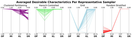
Figure 24.
Parallel coordinates plots showing the results for a subset of sampling algorithms: clustered partitioning, Hansch Controlled, Grid Simple, and Random Stratified. Each line represents one of the 72 averaged experiment trials for each algorithm. The y-axes correspond to the four measured characteristics: overlap percentage (OP), Moran’s I (MI), KL divergence (KL), and difference ratio (DR), with values normalized and scaled globally across all experiments. Algorithms with lines trending toward the top of the plots indicate more desirable outcomes.
Figure 24 presents a parallel coordinates plot for each of the representative sampling algorithms. Each line in the subplots corresponds to one of the 72 averaged experiment trials for each algorithm. The y-axes represent the four desirable characteristic measurements, with shared ranges across all subplots, scaled globally across all experiment results. Additionally, the y-axes were normalized and oriented so that more desirable values are higher and less desirable values are lower. As a result, subplots with lines trending toward the top of the plot area indicate more desirable outcomes, while those lower indicate less desirable outcomes.
In Figure 24, we observe varying performance across the four representative sampling algorithms. Each plot highlights different trends in the desirable characteristics, helping us evaluate how well each algorithm avoids inducing bias in empirical error calculations during model development. Moreover, the empirical results for each algorithm align with the theoretical descriptions provided in Section 3.1.5.
The results for Random Stratified show undesirable and tightly bounded OP and MI values, indicating a high amount of overlap correlation and local spatial autocorrelation. OP values tend toward 100%, which occurs because the algorithm does not control for the proximity of training and testing CPLs, often placing them as direct rook neighbors. The MI values are all approximately 0, reflecting the low global spatial autocorrelation caused by the random placement of CPLs. However, due to the stratified selection of CPLs, the algorithm achieves near-perfect KL values across all experiments. Additionally, because the algorithm uses to calculate the number of CPLs per class in each stratum, it also achieves near-perfect DR values. Overall, Random Stratified, like most random-type sampling methods, is not suitable for model development due to the high overlap and local spatial autocorrelation it allows.
Grid Simple also shows tightly bounded OP and MI values. Unlike Random Stratified, its OP values are desirable, but its MI values are not. Since we did not enable strided grid positions, no patch overlap occurred, resulting in OP values of 0% for all experiments. However, similar to Random Stratified, the random selection of CPLs (specified by the grid coordinates) results in MI values near 0, indicating low global spatial autocorrelation. Furthermore, the grid-based CPL selection leads to widely varying KL values, as the algorithm cannot consistently match class distributions in the training and testing sets. Despite this, Grid Simple achieves near-perfect DR scores due to its use of for the training patch assignment. Like most grid-type algorithms, Grid Simple is not well-suited for model development due to the substantial local spatial autocorrelation it permits.
The results for Hansch Controlled (Figure 24) show consistently desirable OP values, all at 0%, because it completely prevents overlap between the training and testing sets, effectively eliminating overlap correlation. Along with Acquarelli Controlled, it is the only controlled-type method that fully mitigates overlap. The MI values are also desirable, with many close to 1.0, indicating strong global spatial autocorrelation. This is because the Hansch Controlled method clusters each class into two groups, using one for training CPL selection and the other for testing, thereby spatially separating the training and testing patches.
However, the variation in MI values stems from intrinsic spatial relationships within the datasets. Specifically, training clusters from different classes may be located near each other, reducing spatial separation. This issue becomes more pronounced in datasets with a low percentage of labeled pixel locations. As the number of labeled pixels decreases, the likelihood of neighboring clusters from the same set increases. This pattern is evident in our experiments, particularly in datasets with fewer labeled pixels, as shown in the right-hand subplot of Figure 25. Here, datasets with fewer labeled pixels exhibit lower MI values (closer to 0), while those with more labeled pixels show higher MI values (closer to 1).
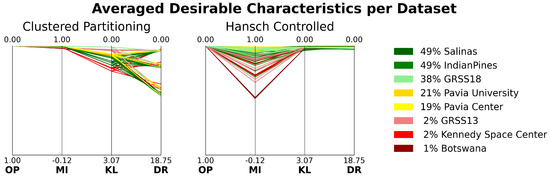
Figure 25.
Parallel coordinates plots showing the averaged results for clustered partitioning and Hansch Controlled sampling algorithms, broken down by dataset. Each line represents one of the 72 averaged experiment trials per dataset, with color coding indicating the percentage of labeled pixels in each dataset. Applying Hansch Controlled to datasets with fewer labeled pixels results in undesirable MI values. Applying clustered partitioning to datasets with fewer labeled pixels results in undesirable KL values.
The KL and DR values of Hansch Controlled are also desirable, as the algorithm selects CPLs from the training clusters in a manner similar to Random Stratified, based on . Overall, Hansch Controlled is well-suited for model development because it minimizes local spatial autocorrelation and eliminates overlap correlation. Other controlled-type algorithms can also be suitable but may lead to low to moderate levels of both types of correlation.
Clustered partitioning (Figure 24) shows desirable and tightly clustered OP and MI values, indicating no overlap correlation and minimal local spatial autocorrelation. The OP values are consistently 0% because the algorithm invalidates all CPLs within a distance of from the partition boundary, effectively preventing patch overlap. The MI values are nearly 1.0 across all experiments, reflecting the selection of patches from spatially disjoint partitions, which ensures strong global spatial autocorrelation.
However, like Hansch Controlled, clustered partitioning is influenced by the intrinsic spatial relationships within datasets. Since the partition boundaries are deterministically computed for each dataset, the resulting partitions have fixed class distributions. If these distributions do not match the empirical distribution of the dataset, non-zero KL values will result. This effect becomes more pronounced in datasets with a low percentage of labeled pixels, where the smaller number of samples within each partition’s class distribution leads to larger KL values. This pattern can be seen in the left-hand subplot of Figure 25, where datasets with fewer labeled pixels show higher KL values.
Similarly, the deterministic class distributions and fixed CPL counts within partitions result in static realizable values. Any requested value that deviates from the fixed distribution will produce non-zero DR values. This is evident in Figure 25, where the three groupings of DR values display an even distribution of dataset representation. The DR value varies with , creating three distinct groupings based on how closely the requested aligns with the partition’s class distribution.
Overall, clustered partitioning, like most partitioning-type sampling methods, is well-suited for model development because it minimizes both local spatial autocorrelation and overlap correlation.
4. Discussion
In this study, we focused specifically on the desirable characteristics of sampling algorithms that address issues related to correlation, particularly the bias introduced by the overlap between training and testing patches and the influence of spatial autocorrelation. While these characteristics are important for assessing the impact of correlation on model performance, it is necessary to recognize that other generally desirable characteristics of sampling methods were not discussed or measured here. However, based on the results, partitioning-type and controlled-type sampling algorithms, such as clustered partitioning and Hansch Controlled, are well suited for model development when the goal is to reduce correlation-induced bias in empirical error. In contrast, random-type and grid-type algorithms tend to allow higher levels of overlap correlation and local spatial autocorrelation, making them less suitable for these purposes. However, we emphasize that this suitability is highly context-dependent, and no single algorithm or type universally provides optimal performance due to the inherent complexity and variability in remote sensing data. It is important to note that each model development task requires careful consideration of both the issues addressed here and other factors when selecting a sampling algorithm.
These results do not suggest that random-type and grid-type sampling methods are inherently unsuitable. With appropriate modifications, both types—along with partitioning and controlled methods—can be adapted to fit specific scenarios. Instead, our findings underscore the necessity of tailoring and adapting sampling approaches specifically to each unique scenario. For example, if overlap correlation is properly managed in a random-type sampling algorithm, larger patch sizes are used, and patches are sampled more sparingly, both forms of correlation could be significantly reduced. Grid-type methods could be improved by avoiding random CPL selection and opting for a more controlled approach, which would help reduce local spatial autocorrelation. Thus, the critical takeaway is that effective sampling strategy selection is a nuanced process requiring detailed consideration of multiple context-specific factors rather than adherence to generalizable guidelines. In general, by addressing the issues of correlation and applying existing mitigation strategies, any of the described sampling methods could potentially be modified to suit different model development instances.
While we believe the findings of this work provide considerable contributions to the field, there are many unaddressed complications and challenges that we did not address. The reasons these were not addressed are due to their complicated effect on the issues and topics negotiated in this work, which is quite lengthy as is. In the following section, we discuss many of the unaddressed challenges we identified. We further note that this is not an exhaustive list, we believe there are many other complications that we have not yet identified that can have a bearing on sampling algorithm and model development design decisions.
Unaddressed Complications and Challenges
We used qualitative terms like small, medium, and large to describe dataset sizes because correlation issues are complex and not solely determined by size. While spatial autocorrelation decreases with distance and thus with larger datasets, overlap correlation does not diminish similarly. Large datasets can still exhibit significant overlap correlation, particularly when images are larger than the patch size and contain multiple patches. Therefore, correlation issues are tied more to image and patch characteristics than to dataset size alone.
The thresholds at which spatial autocorrelation effects become negligible are unclear. Likewise, we do not know how large a dataset must be, or how much overlap correlation it can have before the impact on model assessment is minimal. Identifying specific benchmarks in terms of pixels, images, or classes is challenging.
Most of the machine learning tasks we addressed focus on semantic segmentation, with a few exceptions like height prediction [75,76]. Semantic segmentation naturally involves patch creation, making related articles easier to identify. However, tasks other than semantic segmentation that use patches are harder to pinpoint. Any task requiring patches smaller than the image size can introduce a correlation between training and testing sets, but we did not address this due to the difficulty in identifying such articles.
We did not discuss the distinction between classification and semantic segmentation in data processing and error estimation. Traditionally, remote sensing models performed single-pixel classification by predicting labels from individual pixels or small patches. With the rise of CNNs and GPGPU computing, semantic segmentation became standard, where models ingest larger patches and predict labels for every pixel in the input.
In single-pixel classification, predicting one label does not affect others, and model assessment is straightforward. In semantic segmentation, overlapping testing patches and post-processing methods like voting can complicate assessment. If a testing patch overlaps with training data, its predictions can influence those of a testing-only patch, introducing correlation. Careful post-processing is needed to avoid this issue.
There are several ways in which pre-processing and post-processing steps can influence correlation. For example, removing labels of overlapping pixels (and setting them as unlabeled [69,70]) is inadequate because models still utilize their spectral values during training, thereby maintaining correlation. Secondly, zeroing out or replacing spectral values of overlapping pixels might seem helpful, but its effects are unclear and require careful study. Thirdly, global filtering during pre-processing can inadvertently introduce or worsen correlation, as explored by Liang et al. [77].
Remote sensing datasets are often only partially labeled; in our work, datasets ranged from 0.8% to 48% labeled. This leads to many patches with unlabeled pixels. It is unclear whether overlap at unlabeled pixel locations contributes to correlation. Some CNN loss functions ignore unlabeled pixels in the loss calculation [73,74], but convolution still uses all pixels to learn filters. Other methods may handle this differently, suggesting that specific combinations of methods and allowable unlabeled pixel overlap could lead to optimal, case-specific sampling strategies.
We focused on creating and evaluating training and testing data, not on validation data for model selection. This is because most surveyed works did not mention validation data, and modifying sampling methods to produce a validation set without adding correlation issues is challenging. A validation set would need a low correlation with both the training and testing sets to avoid biased model selection and to provide meaningful estimates of generalizability.
Additionally, while this work focused on structural characteristics of sampling methods and their impact on correlation, we acknowledge that some methods may exhibit sensitivity to user-defined parameters such as patch size, grid stride, or clustering behavior. These effects are not deeply explored here but are worth investigating in future studies, particularly in terms of their influence on overlap and spatial autocorrelation under different dataset configurations.
5. Conclusions
Waldo Tobler described the First Law of Geography as “everything is related to everything else, but near things are more related than distant things” [78]. The assertion underscores the fundamental principle of spatial dependency in geography, geostatistics, and spatial statistics, emphasizing that the degree of relatedness between entities increases with proximity, thereby constraining the analysis and interpretation of spatial data. This study provides strong evidence that this idea requires more consideration when developing machine learning models within this highly related field.
We encourage interested readers to begin with the comprehensive theoretical survey by Nikparvar et al. [79], which provides a broad overview of the relevant concepts. Additionally, Zhang et al. [16] offer a valuable practical perspective by examining six regression models in a real-world setting, making it an excellent resource for those looking to see the application of these ideas in practice and their parallels to the challenges discussed in this study.
In addition to our general recommendation for increased consideration of spatial dependency in remote sensing research, the results of our survey point to specific, actionable steps that can be implemented immediately. First and foremost, it is essential to provide a clear and detailed description of how training and testing data are generated and used during practical applications. The high number of survey articles that offered only partial documentation of their sampling methods underscores the need for this recommendation. Clear documentation is vital for scientific repeatability; without it, replicating previous work to build upon existing knowledge becomes challenging, if not impossible.
Following this, we strongly recommend that researchers explicitly state any biases resulting from the sampling process that may affect the reported empirical results. While acknowledging the potential for correlation is an important first step, it is not sufficient on its own. Future researchers need this information to accurately compare their results with previous works. Without such transparency, it becomes difficult to steer the field toward continual improvement. The lack of a level playing field in comparing model development methodologies could even discourage further research, as consistently positive results (stemming from highly correlated training and testing data) may create the false impression that the field has stagnated at a local optimum.
Finally, we recommend that researchers re-engage with the statistical foundations of machine learning to ensure greater rigor in its application. By doing so, the field can advance more confidently, grounded in a thorough understanding of both the challenges and the potential of machine learning in the context of spatial data.
Author Contributions
Conceptualization, K.T.D. and B.J.B.; methodology, K.T.D.; software, K.T.D.; validation, K.T.D. and B.J.B.; formal analysis, K.T.D.; investigation, K.T.D.; resources, K.T.D.; data curation, K.T.D.; writing—original draft preparation, K.T.D.; writing—review and editing, K.T.D. and B.J.B.; visualization, K.T.D.; supervision, B.J.B.; project administration, K.T.D. and B.J.B. All authors have read and agreed to the published version of the manuscript.
Funding
This research received no external funding.
Data Availability Statement
All code and data are available at https://github.com/kevindckr/samplify (accessed on 8 April 2025).
Acknowledgments
K. Decker thanks B. Borghetti for his guidance, along with his wife, daughter, and parents for their continued support. The views expressed in this article are those of the author and do not necessarily reflect the official policy or position of the Air Force, the Department of Defense, or the U.S. Government.
Conflicts of Interest
The authors declare no conflicts of interest.
Appendix A. Survey Procedures Flowchart
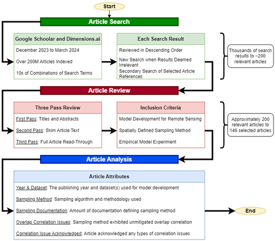
Figure A1.
Flowchart summarizing the systematic review procedure. This diagram illustrates the sequential steps taken during the article search, review, and analysis, explicitly highlighting the inclusion criteria applied during the multi-pass article screening. The final selection of 146 relevant articles resulted from this structured workflow.
Appendix B. Tables of Survey Article References by Attribute Type
Table A1.
Articles per year.
Table A1.
Articles per year.
| Year | Count | References |
|---|---|---|
| 2015 | 12 | [39,80,81,82,83,84,85,86,87,88,89,90] |
| 2016 | 10 | [7,38,91,92,93,94,95,96,97,98] |
| 2017 | 18 | [71,77,99,100,101,102,103,104,105,106,107,108,109,110,111,112,113,114] |
| 2018 | 24 | [11,46,49,58,59,62,67,115,116,117,118,119,120,121,122,123,124,125,126,127,128,129,130,131] |
| 2019 | 19 | [40,54,56,132,133,134,135,136,137,138,139,140,141,142,143,144,145,146,147] |
| 2020 | 13 | [35,41,48,51,53,55,60,61,75,148,149,150,151] |
| 2021 | 16 | [43,45,50,52,63,64,76,152,153,154,155,156,157,158,159,160] |
| 2022 | 20 | [26,27,28,37,44,65,68,69,70,161,162,163,164,165,166,167,168,169,170,171] |
| 2023 | 14 | [36,42,47,57,66,72,172,173,174,175,176,177,178,179] |
Table A2.
Articles per sampler type.
Table A2.
Articles per sampler type.
| Sampler | Count | References |
|---|---|---|
| Acquarelli Controlled | 1 | [46] |
| Clark Stratified | 1 | [66] |
| Grid | 6 | [35,45,61,62,64,65] |
| Hansch Controlled | 1 | [37] |
| Liu Random | 1 | [27] |
| Random Equal | 44 | [26,28,38,63,71,76,77,84,92,97,98,99,100,102,104,105,106,107,110,115,116,122,123,124,126,127,128,129,131,134,138,140,141,142,148,151,154,155,159,160,162,163,173,177] |
| Random GRSS13 | 19 | [44,80,83,86,101,109,117,132,135,145,146,153,157,158,165,166,170,172,175] |
| Random Stratified | 44 | [7,11,43,67,68,69,70,72,81,82,87,88,89,91,93,94,95,96,103,108,111,112,113,114,118,119,120,121,125,130,133,136,137,139,143,144,147,149,150,161,167,168,169,176] |
| Spatial Partitioning | 17 | [36,39,40,41,42,49,50,51,52,53,54,55,56,57,58,59,60] |
| Unknown | 10 | [75,85,90,152,156,164,171,174,178,179] |
| Zhang Grid | 1 | [47] |
| Zou Grid | 1 | [48] |
Table A3.
Articles per sampler documentation.
Table A3.
Articles per sampler documentation.
| Documentation Amount | Count | References |
|---|---|---|
| Full | 7 | [27,47,48,52,66,67,68] |
| No | 12 | [64,65,75,89,90,117,152,156,164,174,178,179] |
| Partial | 127 | [7,11,26,28,35,36,37,38,39,40,41,42,43,44,45,46,49,50,51,53,54,55,56,57,58,59,60,61,62,63,69,70,71,72,76,77,80,81,82,83,84,85,86,87,88,91,92,93,94,95,96,97,98,99,100,101,102,103,104,105,106,107,108,109,110,111,112,113,114,115,116,118,119,120,121,122,123,124,125,126,127,128,129,130,131,132,133,134,135,136,137,138,139,140,141,142,143,144,145,146,147,148,149,150,151,153,154,155,157,158,159,160,161,162,163,165,166,167,168,169,170,171,172,173,175,176,177] |
Table A4.
Articles per correlation issue present.
Table A4.
Articles per correlation issue present.
| Issue Present | Count | References |
|---|---|---|
| No | 27 | [27,36,39,40,41,42,43,44,45,46,47,48,49,50,51,52,53,54,55,56,57,58,59,60,61,62,63] |
| Unknown | 49 | [7,35,37,64,69,70,75,81,83,84,85,86,87,89,95,96,98,102,103,104,107,109,112,113,114,115,119,123,126,127,137,138,139,140,146,148,152,156,159,162,164,167,168,169,171,174,177,178,179] |
| Yes | 70 | [11,26,28,38,65,66,67,68,71,72,76,77,80,82,88,90,91,92,93,94,97,99,100,101,105,106,108,110,111,116,117,118,120,121,122,124,125,128,129,130,131,132,133,134,135,136,141,142,143,144,145,147,149,150,151,153,154,155,157,158,160,161,163,165,166,170,172,173,175,176] |
Table A5.
Articles per correlation issue acknowledgment.
Table A5.
Articles per correlation issue acknowledgment.
| Acknowledged | Count | References |
|---|---|---|
| No | 132 | [7,11,26,28,35,49,50,51,52,53,54,55,56,57,58,59,60,61,62,63,64,65,66,67,68,69,70,71,72,75,76,77,80,81,82,83,84,85,86,87,88,89,90,91,92,93,94,95,96,97,98,99,100,101,102,103,104,105,106,107,108,109,110,111,112,113,114,115,116,117,118,119,120,121,122,123,124,125,126,127,128,129,130,131,132,133,134,135,136,137,138,139,140,141,142,143,144,145,146,147,148,149,150,151,152,153,154,155,156,157,158,159,160,161,162,163,164,165,166,167,168,169,170,171,172,173,174,175,176,177,178,179] |
| Yes | 14 | [27,36,37,38,39,40,41,42,43,44,45,46,47,48] |
Table A6.
Articles per issue acknowledgment and overlap correlation.
Table A6.
Articles per issue acknowledgment and overlap correlation.
| Acknowledged | Issue Present | Count | References |
|---|---|---|---|
| No | No | 15 | [49,50,51,52,53,54,55,56,57,58,59,60,61,62,63] |
| No | Unknown | 48 | [7,35,64,69,70,75,81,83,84,85,86,87,89,95,96,98,102,103,104,107,109,112,113,114,115,119,123,126,127,137,138,139,140,146,148,152,156,159,162,164,167,168,169,171,174,177,178,179] |
| No | Yes | 69 | [11,26,28,65,66,67,68,71,72,76,77,80,82,88,90,91,92,93,94,97,99,100,101,105,106,108,110,111,116,117,118,120,121,122,124,125,128,129,130,131,132,133,134,135,136,141,142,143,144,145,147,149,150,151,153,154,155,157,158,160,161,163,165,166,170,172,173,175,176] |
| Yes | No | 12 | [27,36,39,40,41,42,43,44,45,46,47,48] |
| Yes | Unknown | 1 | [37] |
| Yes | Yes | 1 | [38] |
Table A7.
Articles per dataset (A–K).
Table A7.
Articles per dataset (A–K).
| Dataset | Count | References |
|---|---|---|
| AIRS | 1 | [152] |
| AlexandraCanal | 1 | [65] |
| Alto Tajo | 1 | [81] |
| Ausburg | 2 | [176,177] |
| Bayview Park | 2 | [82,100] |
| Berlin | 2 | [173,176] |
| Big Pines | 1 | [144] |
| Botswana | 3 | [26,77,96] |
| Brookings | 1 | [54] |
| Cerrado | 1 | [36] |
| Chendu | 1 | [61] |
| Dordogne | 1 | [43] |
| Finland | 1 | [164] |
| Flevoland | 1 | [37] |
| GRSS07 | 1 | [166] |
| GRSS13 | 49 | [26,28,39,44,48,54,60,63,68,80,83,86,92,97,100,101,107,109,117,120,126,127,128,131,132,133,135,141,145,146,147,151,153,155,157,158,159,164,165,166,168,170,171,172,173,175,176,177,178] |
| GRSS14 | 4 | [123,136,163,169] |
| GRSS17 | 1 | [70] |
| GRSS18 | 32 | [26,40,41,42,47,49,50,51,54,55,56,58,59,60,70,75,76,118,140,148,152,154,157,158,162,167,171,173,174,175,178,179] |
| GRSS22 | 1 | [72] |
| Galveston | 1 | [126] |
| GeoManitoba | 1 | [35] |
| Guangzhou | 1 | [62] |
| Hanover | 1 | [178] |
| Harbin | 2 | [123,136] |
| HoustonCity | 1 | [64] |
| Huelva | 1 | [81] |
| INRIA | 1 | [152] |
| ISPRS Potsdam | 2 | [62,152] |
| ISPRS Vaihingen | 3 | [75,76,152] |
| ISPRS Vaihingen3D | 1 | [53] |
| Indian Pines | 57 | [7,11,26,27,28,42,46,47,48,67,68,71,77,84,88,93,94,95,96,98,99,102,103,104,105,106,107,108,110,111,112,113,114,116,119,120,121,124,125,129,130,133,136,138,139,143,144,147,149,150,155,160,161,167,168,169,172] |
| KSC Florida | 11 | [27,46,93,99,108,112,115,130,143,144,160] |
| KermanCity | 1 | [137] |
Table A8.
Articles per dataset (L–Y).
Table A8.
Articles per dataset (L–Y).
| Dataset | Count | References |
|---|---|---|
| LCZ | 1 | [175] |
| LCZHongKong | 1 | [177] |
| LocalClimateZones | 1 | [52] |
| MUUFL | 3 | [151,159,165] |
| Matiwan | 1 | [162] |
| MiniFrance | 1 | [72] |
| NISAR | 1 | [156] |
| Nashua | 1 | [178] |
| Oberpfaffenhofen | 1 | [37] |
| Osaka | 1 | [56] |
| Pavia Center | 16 | [38,46,52,60,71,84,88,89,91,96,106,115,122,142,149,154] |
| Pavia University | 66 | [11,26,27,28,38,42,46,48,52,60,67,68,71,77,85,88,89,90,91,93,94,95,98,102,103,104,105,106,107,108,110,112,113,114,115,116,119,120,121,122,124,125,126,128,129,130,131,134,136,138,139,142,143,144,147,149,150,154,155,160,161,162,163,168,169,172] |
| Queensland | 1 | [66] |
| Recology | 2 | [82,100] |
| ReunionIsland | 1 | [43] |
| Rio Tinto | 1 | [164] |
| Rochester | 1 | [141] |
| Salinas | 32 | [27,28,46,47,48,71,84,88,99,102,103,104,105,106,110,114,116,120,125,128,129,134,139,143,144,147,150,154,157,163,168,169] |
| ShenzhenDongguan | 1 | [45] |
| ShirazCity | 1 | [137] |
| Tabada | 1 | [81] |
| Toronto | 1 | [87] |
| Trento | 9 | [44,101,109,128,146,151,164,165,166] |
| VEDAI | 1 | [152] |
| Vancouver | 1 | [69] |
| Vancouver Harbor | 1 | [69] |
| WUSU | 1 | [57] |
| Washington | 2 | [133,161] |
| Wertheim | 1 | [153] |
| XJTU | 1 | [69] |
| Xian South | 1 | [69] |
| Yancheng | 1 | [60] |
| YellowRiver | 1 | [162] |
Appendix C. Extended Empirical Results Figure
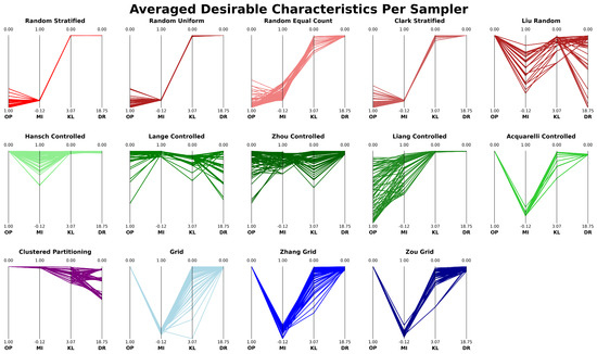
Figure A2.
Parallel coordinates plots showing the results for all sampling algorithms. Each line represents 1 of the 72 averaged experiment trials for each algorithm. The y-axes correspond to the four measured characteristics: overlap percentage (OP), Moran’s I (MI), KL divergence (KL), and difference ratio (DR), with values normalized and scaled globally across all experiments. Algorithms with lines trending toward the top of the plots indicate more desirable outcomes.
Appendix C.1. Representative Sampling Algorithm Selection
The appendix in Figure A2 presents the empirical results for all the sampling methods discussed in Section 3.4. As noted, a subset of the available and tested sampling algorithms was selected for presentation in Section 3.4, with further discussion on the subset provided here.
All random-type sampling algorithms (shades of red in Figure A2) produce nearly identical results, except for Liu Random. Liu Random differs because it prevents overlap correlation by enforcing a P boundary around training patches, resulting in a 0% overlap. Additionally, Liu Random selects only one patch per class for the training set, leading to a highly imbalanced number of samples between the training and testing sets. As a result, the global spatial autocorrelation, measured by Moran’s I, is very high. Furthermore, Liu Random is poorly documented, as discussed in Section 3.1.8, and our interpretation of its description finds it poorly motivated. Therefore, Random Stratified was chosen as the representative random-type sampling method, as it produces nearly identical results to the other random-type methods and was the most frequently cited during the literature survey.
Similarly, all grid-type sampling algorithms (shades of blue in Figure A2) yield nearly identical results. Zhang Grid and Zhou Grid achieved slightly more balanced KL divergence between the training class distribution and the dataset’s empirical class distribution due to their patch selection strategies. However, in terms of the other three measured characteristics, all grid-type samplers performed identically. Grid Simple was selected as the representative grid-type method because it is the simplest and easiest to understand.
The controlled-type sampling algorithms (shades of green in Figure A2) do not produce identical results. To select a representative sampler, we first excluded methods that did not fully mitigate the overlap correlation (Lange Controlled, Zhou Controlled, and Liang Controlled). This was done for two reasons: first, the overlap correlation introduces a stronger bias toward the empirical error; second, it is relatively straightforward to fully eliminate overlap correlation. Acquarelli Controlled was also excluded because, like Liu Random, it was poorly documented and poorly motivated. This left Hasnch Controlled as the representative controlled-type sampling method.
Finally, as discussed in Section 3.1.11, we did not identify any other automated partitioning-type sampling methods for testing. The only partitioning-type sampling algorithm provided is described in this work. Consequently, clustered partitioning was selected as the representative partitioning-type sampling method.
References
- Friedl, M.A.; Woodcock, C.; Gopal, S.; Muchoney, D.; Strahler, A.H.; Barker-Schaaf, C. A note on procedures used for accuracy assessment in land cover maps derived from AVHRR data. Int. J. Remote Sens. 2000, 21, 1073–1077. [Google Scholar] [CrossRef]
- Zhen, Z.; Quackenbush, L.J.; Stehman, S.V.; Zhang, L. Impact of training and validation sample selection on classification accuracy and accuracy assessment when using reference polygons in object-based classification. Int. J. Remote Sens. 2013, 34, 6914–6930. [Google Scholar] [CrossRef]
- Zhou, J.; Liang, J.; Qian, Y.; Gao, Y.; Tong, L. On the sampling strategies for evaluation of joint spectral-spatial information based classifiers. In Proceedings of the Workshop on Hyperspectral Image and Signal Processing, Evolution in Remote Sensing, Tokyo, Japan, 2–5 June 2015. [Google Scholar] [CrossRef]
- Liang, J.; Zhou, J.; Qian, Y.; Wen, L.; Bai, X.; Gao, Y. On the Sampling Strategy for Evaluation of Spectral-Spatial Methods in Hyperspectral Image Classification. IEEE Trans. Geosci. Remote Sens. 2017, 55, 862–880. [Google Scholar] [CrossRef]
- Hansch, R.; Ley, A.; Hellwich, O. Correct and still wrong: The relationship between sampling strategies and the estimation of the generalization error. In Proceedings of the International Geoscience and Remote Sensing Symposium (IGARSS), Fort Worth, TX, USA, 23–28 July 2017; pp. 3672–3675. [Google Scholar] [CrossRef]
- Lange, J.; Cavallaro, G.; Götz, M.; Erlingsson, E.; Riedel, M. The influence of sampling methods on pixel-wise hyperspectral image classification with 3D convolutional neural networks. In Proceedings of the International Geoscience and Remote Sensing Symposium (IGARSS), Valencia, Spain, 22–27 July 2018; pp. 2087–2090. [Google Scholar] [CrossRef]
- Romero, A.; Gatta, C.; Camps-Valls, G. Unsupervised deep feature extraction for remote sensing image classification. IEEE Trans. Geosci. Remote Sens. 2016, 54, 1349–1362. [Google Scholar] [CrossRef]
- Audebert, N.; Saux, B.L.; Lefevre, S. Deep learning for classification of hyperspectral data: A comparative review. IEEE Geosci. Remote Sens. Mag. 2019, 7, 159–173. [Google Scholar] [CrossRef]
- Nalepa, J.; Myller, M.; Kawulok, M. Validating Hyperspectral Image Segmentation. IEEE Geosci. Remote Sens. Lett. 2019, 16, 1264–1268. [Google Scholar] [CrossRef]
- Hänsch, R. The Trap of Random Sampling and How to Avoid It: Alternative Sampling Strategies for a Realistic Estimate of the Generalization Error in Remote Sensing. In Proceedings of the International Geoscience and Remote Sensing Symposium (IGARSS), Brussels, Belgium, 11–16 July 2021; pp. 2020–2023. [Google Scholar] [CrossRef]
- Cao, X.; Zhou, F.; Xu, L.; Meng, D.; Xu, Z.; Paisley, J. Hyperspectral Image Classification with Markov Random Fields and a Convolutional Neural Network. IEEE Trans. Image Process. 2018, 27, 2354–2367. [Google Scholar] [CrossRef]
- Shih, C.Y.; Teicher, H. Probability Theory. Independence, Interchangeability, Martingales, 3rd ed.; Springer Texts in Statistics; Springer: Berlin/Heidelberg, Germany, 1997. [Google Scholar]
- Encyclopedia of Mathematics. De Finetti Theorem. Available online: https://encyclopediaofmath.org/index.php?title=De_Finetti_theorem (accessed on 24 August 2024).
- Goodfellow, I.; Bengio, Y.; Courville, A. Deep Learning; MIT Press: Cambridge, MA, USA, 2016; Available online: http://www.deeplearningbook.org (accessed on 5 July 2024).
- He, H.; Garcia, E.A. Learning from imbalanced data. IEEE Trans. Knowl. Data Eng. 2009, 21, 1263–1284. [Google Scholar] [CrossRef]
- Zhang, L.; Ma, Z.; Guo, L. An Evaluation of Spatial Autocorrelation and Heterogeneity in the Residuals of Six Regression Models. For. Sci. 2009, 55, 533–548. [Google Scholar] [CrossRef]
- Moran, P.A.P. Notes on Continuous Stochastic Phenomena. Biometrika 1950, 37, 17. [Google Scholar] [CrossRef]
- Kullback, S.; Leibler, R.A. On Information and Sufficiency. Ann. Math. Stat. 1951, 22, 79–86. [Google Scholar] [CrossRef]
- Hyperspectral Image Analysis Lab, University of Houston. 2018 IEEE GRSS Data Fusion Challenge–Fusion of Multispectral LiDAR and Hyperspectral Data. Available online: https://machinelearning.ee.uh.edu/2018-ieee-grss-data-fusion-challenge-fusion-of-multispectral-lidar-and-hyperspectral-data/ (accessed on 1 December 2022).
- Grana, M.; Veganzons, M.A.; Ayerdi, B. Hyperspectral Remote Sensing Scenes–Grupo de Inteligencia Computacional (GIC). Available online: https://www.ehu.eus/ccwintco/index.php/Hyperspectral_Remote_Sensing_Scenes (accessed on 14 August 2024).
- Deng, W. GRSS HOS MAT. 2021. Dataset on Figshare. Available online: https://doi.org/10.6084/m9.figshare.16528845.v1 (accessed on 14 August 2024).
- Xu, Y.; Du, B.; Zhang, L.; Cerra, D.; Pato, M.; Carmona, E.; Prasad, S.; Yokoya, N.; Hansch, R.; Le Saux, B. Advanced multi-sensor optical remote sensing for urban land use and land cover classification: Outcome of the 2018 ieee grss data fusion contest. IEEE J. Sel. Top. Appl. Earth Obs. Remote Sens. 2019, 12, 1709–1724. [Google Scholar] [CrossRef]
- Debes, C.; Merentitis, A.; Heremans, R.; Hahn, J.; Frangiadakis, N.; Van Kasteren, T.; Liao, W.; Bellens, R.; Pizurica, A.; Gautama, S.; et al. Hyperspectral and LiDAR data fusion: Outcome of the 2013 GRSS data fusion contest. IEEE J. Sel. Top. Appl. Earth Obs. Remote Sens. 2014, 7, 2405–2418. [Google Scholar] [CrossRef]
- Huang, X.; Zhang, L. A comparative study of spatial approaches for urban mapping using hyperspectral ROSIS images over Pavia City, northern Italy. Int. J. Remote Sens. 2009, 30, 3205–3221. [Google Scholar] [CrossRef]
- Mura, M.D.; Benediktsson, J.A.; Chanussot, J.; Bruzzone, L. The Evolution of the Morphological Profile: From Panchromatic to Hyperspectral Images. In Optical Remote Sensing; Springer: Berlin/Heidelberg, Germany, 2011; pp. 123–146. [Google Scholar] [CrossRef]
- Yu, D.; Li, Q.; Wang, X.; Xu, C.; Zhou, Y. A Cross-Level Spectral-Spatial Joint Encode Learning Framework for Imbalanced Hyperspectral Image Classification. IEEE Trans. Geosci. Remote Sens. 2022, 60, 5411717. [Google Scholar] [CrossRef]
- Liu, X.; Gong, X.; Plaza, A.; Cai, Z.; Xiao, X.; Jiang, X.; Liu, X. MO-CNN: Multiobjective Optimization of Convolutional Neural Networks for Hyperspectral Image Classification. IEEE Trans. Geosci. Remote Sens. 2022, 60, 5543314. [Google Scholar] [CrossRef]
- Yuan, Y.; Wang, C.; Jiang, Z. Proxy-Based Deep Learning Framework for Spectral-Spatial Hyperspectral Image Classification: Efficient and Robust. IEEE Trans. Geosci. Remote Sens. 2022, 60, 5501115. [Google Scholar] [CrossRef]
- Google. Google Scholar. Available online: https://scholar.google.com/ (accessed on 1 December 2023).
- Digital Science. Dimensions.ai. Available online: https://app.dimensions.ai/discover/publication (accessed on 1 December 2023).
- Khabsa, M.; Giles, C.L. The Number of Scholarly Documents on the Public Web. PLoS ONE 2014, 9, e93949. [Google Scholar] [CrossRef]
- Cireşan, D.C.; Meier, U.; Gambardella, L.M.; Schmidhuber, J. Deep, Big, Simple Neural Nets for Handwritten Digit Recognition. Neural Comput. 2010, 22, 3207–3220. [Google Scholar] [CrossRef]
- Krizhevsky, A.; Sutskever, I.; Hinton, G.E. ImageNet classification with deep convolutional neural networks. Commun. ACM 2017, 60, 84–90. [Google Scholar] [CrossRef]
- He, K.; Zhang, X.; Ren, S.; Sun, J. Deep residual learning for image recognition. In Proceedings of the IEEE Computer Society Conference on Computer Vision and Pattern Recognition, Las Vegas, NV, USA, 27–30 June 2016; pp. 770–778. [Google Scholar] [CrossRef]
- Alhassan, V.; Henry, C.; Ramanna, S.; Storie, C. A deep learning framework for land-use/land-cover mapping and analysis using multispectral satellite imagery. Neural Comput. Appl. 2020, 32, 8529–8544. [Google Scholar] [CrossRef]
- Filho, P.S.; Persello, C.; Maretto, R.V.; MacHado, R. Investigating Sar-Optical Deep Learning Data Fusion to Map the Brazilian Cerrado Vegetation with Sentinel Data. In Proceedings of the International Geoscience and Remote Sensing Symposium (IGARSS), Pasadena, CA, USA, 16–21 July 2023; pp. 1365–1368. [Google Scholar] [CrossRef]
- Fang, Z.; Zhang, G.; Dai, Q.; Xue, B. PolSAR Image Classification Based on Complex-Valued Convolutional Long Short-Term Memory Network. IEEE Geosci. Remote Sens. Lett. 2022, 19, 4504305. [Google Scholar] [CrossRef]
- Zhao, W.; Du, S. Spectral-Spatial Feature Extraction for Hyperspectral Image Classification: A Dimension Reduction and Deep Learning Approach. IEEE Trans. Geosci. Remote Sens. 2016, 54, 4544–4554. [Google Scholar] [CrossRef]
- Bigdeli, B.; Samadzadegan, F.; Reinartz, P. Fusion of hyperspectral and LIDAR data using decision template-based fuzzy multiple classifier system. Int. J. Appl. Earth Obs. Geoinf. 2015, 38, 309–320. [Google Scholar] [CrossRef]
- Guiotte, F.; Lefevre, S.; Corpetti, T. Rasterization strategies for airborne LiDAR classification using attribute profiles. In Proceedings of the 2019 Joint Urban Remote Sensing Event, JURSE 2019, Vannes, France, 22–24 May 2019. [Google Scholar] [CrossRef]
- Guiotte, F.; Pham, M.T.; Dambreville, R.; Corpetti, T.; Lefevre, S. Semantic Segmentation of LiDAR Points Clouds: Rasterization beyond Digital Elevation Models. IEEE Geosci. Remote Sens. Lett. 2020, 17, 2016–2019. [Google Scholar] [CrossRef]
- Zhang, P.; Yu, H.; Li, P.; Wang, R. TransHSI: A Hybrid CNN-Transformer Method for Disjoint Sample-Based Hyperspectral Image Classification. Remote Sens. 2023, 15, 5331. [Google Scholar] [CrossRef]
- Gbodjo, Y.J.E.; Montet, O.; Ienco, D.; Gaetano, R.; Dupuy, S. Multisensor Land Cover Classification with Sparsely Annotated Data Based on Convolutional Neural Networks and Self-Distillation. IEEE J. Sel. Top. Appl. Earth Obs. Remote Sens. 2021, 14, 11485–11499. [Google Scholar] [CrossRef]
- Hong, D.; Gao, L.; Hang, R.; Zhang, B.; Chanussot, J. Deep Encoder-Decoder Networks for Classification of Hyperspectral and LiDAR Data. IEEE Geosci. Remote Sens. Lett. 2022, 19, 5500205. [Google Scholar] [CrossRef]
- Zhu, Y.; Geis, C.; So, E.; Jin, Y. Multitemporal Relearning with Convolutional LSTM Models for Land Use Classification. IEEE J. Sel. Top. Appl. Earth Obs. Remote Sens. 2021, 14, 3251–3265. [Google Scholar] [CrossRef]
- Acquarelli, J.; Marchiori, E.; Buydens, L.M.; Tran, T.; van Laarhoven, T. Spectral-Spatial Classification of Hyperspectral Images: Three Tricks and a New Learning Setting. Remote Sens. 2018, 10, 1156. [Google Scholar] [CrossRef]
- Zhang, X.; Su, Y.; Gao, L.; Bruzzone, L.; Gu, X.; Tian, Q. A Lightweight Transformer Network for Hyperspectral Image Classification. IEEE Trans. Geosci. Remote Sens. 2023, 61, 5517617. [Google Scholar] [CrossRef]
- Zou, L.; Zhu, X.; Wu, C.; Liu, Y.; Qu, L. Spectral-Spatial Exploration for Hyperspectral Image Classification via the Fusion of Fully Convolutional Networks. IEEE J. Sel. Top. Appl. Earth Obs. Remote Sens. 2020, 13, 659–674. [Google Scholar] [CrossRef]
- Cerra, D.; Pato, M.; Carmona, E.; Azimi, S.M.; Tian, J.; Bahmanyar, R.; Kurz, F.; Vig, E.; Bittner, K.; Henry, C.; et al. Combining deep and shallow neural networks with ad hoc detectors for the classification of complex multi-modal urban scenes. In Proceedings of the International Geoscience and Remote Sensing Symposium (IGARSS), Valencia, Spain, 22–27 July 2018; pp. 3856–3859. [Google Scholar] [CrossRef]
- Hansch, R.; Hellwich, O. Fusion of Multispectral LiDAR, Hyperspectral, and RGB Data for Urban Land Cover Classification. IEEE Geosci. Remote Sens. Lett. 2021, 18, 366–370. [Google Scholar] [CrossRef]
- Hong, D.; Chanussot, J.; Yokoya, N.; Kang, J.; Zhu, X.X. Learning-Shared Cross-Modality Representation Using Multispectral-LiDAR and Hyperspectral Data. IEEE Geosci. Remote Sens. Lett. 2020, 17, 1470–1474. [Google Scholar] [CrossRef]
- Hong, D.; Yao, J.; Meng, D.; Xu, Z.; Chanussot, J. Multimodal GANs: Toward Crossmodal Hyperspectral-Multispectral Image Segmentation. IEEE Trans. Geosci. Remote Sens. 2021, 59, 5103–5113. [Google Scholar] [CrossRef]
- Li, W.; Wang, F.D.; Xia, G.S. A geometry-attentional network for ALS point cloud classification. ISPRS J. Photogramm. Remote Sens. 2020, 164, 26–40. [Google Scholar] [CrossRef]
- Liu, T.; Zhang, X.; Gu, Y. Unsupervised cross-temporal classification of hyperspectral images with multiple geodesic flow kernel learning. IEEE Trans. Geosci. Remote Sens. 2019, 57, 9688–9701. [Google Scholar] [CrossRef]
- Nock, K.; Gilmour, E. Fuzzy aggregation for multimodal remote sensing classification. In Proceedings of the 2020 IEEE International Conference on Fuzzy Systems (FUZZ-IEEE), Glasgow, UK, 19–24 July 2020. [Google Scholar] [CrossRef]
- Poliyapram, V.; Wang, W.; Nakamura, R. A Point-Wise LiDAR and Image Multimodal Fusion Network (PMNet) for Aerial Point Cloud 3D Semantic Segmentation. Remote Sens. 2019, 11, 2961. [Google Scholar] [CrossRef]
- Shi, S.; Zhong, Y.; Liu, Y.; Wang, J.; Wan, Y.; Zhao, J.; Lv, P.; Zhang, L.; Li, D. Multi-temporal urban semantic understanding based on GF-2 remote sensing imagery: From tri-temporal datasets to multi-task mapping. Int. J. Digit. Earth 2023, 16, 3321–3347. [Google Scholar] [CrossRef]
- Sukhanov, S.; Budylskii, D.; Tankoyeu, I.; Heremans, R.; Debes, C. Fusion of LiDar, hyperspectral and RGB data for urban land use and land cover classification. In Proceedings of the International Geoscience and Remote Sensing Symposium (IGARSS), Valencia, Spain, 22–27 July 2018; pp. 3864–3867. [Google Scholar] [CrossRef]
- Xu, Y.; Du, B.; Zhang, L. Multi-source remote sensing data classification via fully convolutional networks and post-classification processing. In Proceedings of the International Geoscience and Remote Sensing Symposium (IGARSS), Valencia, Spain, 22–27 July 2018; pp. 3852–3855. [Google Scholar] [CrossRef]
- Yang, W.; Peng, J.; Sun, W. Ideal Regularized Discriminative Multiple Kernel Subspace Alignment for Domain Adaptation in Hyperspectral Image Classification. IEEE J. Sel. Top. Appl. Earth Obs. Remote Sens. 2020, 13, 5833–5846. [Google Scholar] [CrossRef]
- Li, M.J.; Zhu, M.C.; Ma, Z.; Li, P.S.; Zhang, X.B.; Hou, A.K.; Shi, J.B.; He, Y.; Chen, K.; Weng, T.; et al. Classification of Surface Natural Resources based on U-NET and GF-1 Satellite Images. In Proceedings of the 2020 17th International Computer Conference on Wavelet Active Media Technology and Information Processing, ICCWAMTIP 2020, Chengdu, China, 18–20 December 2020; pp. 179–182. [Google Scholar] [CrossRef]
- Sun, Y.; Zhang, X.; Xin, Q.; Huang, J. Developing a multi-filter convolutional neural network for semantic segmentation using high-resolution aerial imagery and LiDAR data. ISPRS J. Photogramm. Remote Sens. 2018, 143, 3–14. [Google Scholar] [CrossRef]
- Hong, D.; Gao, L.; Wu, X.; Yao, J.; Yokoya, N.; Zhang, B. A Unified Multimodal Deep Learning Framework for Remote Sensing Imagery Classification. In Proceedings of the Workshop on Hyperspectral Image and Signal Processing, Evolution in Remote Sensing, Amsterdam, The Netherlands, 24–26 March 2021. [Google Scholar] [CrossRef]
- Garg, R.; Kumar, A.; Bansal, N.; Prateek, M.; Kumar, S. Semantic segmentation of PolSAR image data using advanced deep learning model. Sci. Rep. 2021, 11, 15365. [Google Scholar] [CrossRef] [PubMed]
- Gong, S.; Ball, J.; Surawski, N. Urban land-use land-cover extraction for catchment modelling using deep learning techniques. J. Hydroinform. 2022, 24, 388–405. [Google Scholar] [CrossRef]
- Clark, A.; Phinn, S.; Scarth, P. Optimised U-Net for Land Use–Land Cover Classification Using Aerial Photography. PFG J. Photogramm. Remote Sens. Geoinf. Sci. 2023, 91, 125–147. [Google Scholar] [CrossRef]
- Paoletti, M.E.; Haut, J.M.; Plaza, J.; Plaza, A. A new deep convolutional neural network for fast hyperspectral image classification. ISPRS J. Photogramm. Remote Sens. 2018, 145, 120–147. [Google Scholar] [CrossRef]
- Zhu, Q.; Deng, W.; Zheng, Z.; Zhong, Y.; Guan, Q.; Lin, W.; Zhang, L.; Li, D. A Spectral-Spatial-Dependent Global Learning Framework for Insufficient and Imbalanced Hyperspectral Image Classification. IEEE Trans. Cybern. 2022, 52, 11709–11723. [Google Scholar] [CrossRef]
- Liu, X.; Li, L.; Liu, F.; Hou, B.; Yang, S.; Jiao, L. GAFnet: Group Attention Fusion Network for PAN and MS Image High-Resolution Classification. IEEE Trans. Cybern. 2022, 52, 10556–10569. [Google Scholar] [CrossRef]
- Liu, X.; Jiao, L.; Li, L.; Cheng, L.; Liu, F.; Yang, S.; Hou, B. Deep Multiview Union Learning Network for Multisource Image Classification. IEEE Trans. Cybern. 2022, 52, 4534–4546. [Google Scholar] [CrossRef]
- Yang, J.; Zhao, Y.Q.; Chan, J.C.W. Learning and Transferring Deep Joint Spectral-Spatial Features for Hyperspectral Classification. IEEE Trans. Geosci. Remote Sens. 2017, 55, 4729–4742. [Google Scholar] [CrossRef]
- Cuypers, S.; Nascetti, A.; Vergauwen, M. Land Use and Land Cover Mapping with VHR and Multi-Temporal Sentinel-2 Imagery. Remote Sens. 2023, 15, 2501. [Google Scholar] [CrossRef]
- Decker, K.T.; Borghetti, B.J. Composite Style Pixel and Point Convolution-Based Deep Fusion Neural Network Architecture for the Semantic Segmentation of Hyperspectral and Lidar Data. Remote Sens. 2022, 14, 2113. [Google Scholar] [CrossRef]
- Decker, K.T.; Borghetti, B.J. Hyperspectral Point Cloud Projection for the Semantic Segmentation of Multimodal Hyperspectral and Lidar Data with Point Convolution-Based Deep Fusion Neural Networks. Appl. Sci. 2023, 13, 8210. [Google Scholar] [CrossRef]
- Carvalho, M.; Saux, B.L.; Trouve-Peloux, P.; Champagnat, F.; Almansa, A. Multitask Learning of Height and Semantics from Aerial Images. IEEE Geosci. Remote Sens. Lett. 2020, 17, 1391–1395. [Google Scholar] [CrossRef]
- Elhousni, M.; Zhang, Z.; Huang, X. Height Prediction and Refinement from Aerial Images with Semantic and Geometric Guidance. IEEE Access 2021, 9, 145638–145647. [Google Scholar] [CrossRef]
- Li, Y.; Zhang, H.; Shen, Q. Spectral–Spatial Classification of Hyperspectral Imagery with 3D Convolutional Neural Network. Remote Sens. 2017, 9, 67. [Google Scholar] [CrossRef]
- Tobler, W.R. A Computer Movie Simulating Urban Growth in the Detroit Region. Econ. Geogr. 1970, 46, 234. [Google Scholar] [CrossRef]
- Nikparvar, B.; Thill, J.C. Machine Learning of Spatial Data. ISPRS Int. J. -Geo-Inf. 2021, 10, 600. [Google Scholar] [CrossRef]
- Abbasi, B.; Arefi, H.; Bigdeli, B.; Motagh, M.; Roessne, S. Fusion of hyperspectral and lidar data based on dimension reduction and maximum likelihood. Int. Arch. Photogramm. Remote Sens. Spat. Inf. Sci. 2015, 40, 569–573. [Google Scholar] [CrossRef]
- García-Gutiérrez, J.; Mateos-García, D.; Garcia, M.; Riquelme-Santos, J.C. An evolutionary-weighted majority voting and support vector machines applied to contextual classification of LiDAR and imagery data fusion. Neurocomputing 2015, 163, 17–24. [Google Scholar] [CrossRef]
- Gu, Y.; Wang, Q.; Jia, X.; Benediktsson, J.A. A Novel MKL Model of Integrating LiDAR Data and MSI for Urban Area Classification. IEEE Trans. Geosci. Remote Sens. 2015, 53, 5312–5326. [Google Scholar] [CrossRef]
- Khodadadzadeh, M.; Li, J.; Prasad, S.; Plaza, A. Fusion of Hyperspectral and LiDAR Remote Sensing Data Using Multiple Feature Learning. IEEE J. Sel. Top. Appl. Earth Obs. Remote Sens. 2015, 8, 2971–2983. [Google Scholar] [CrossRef]
- Li, W.; Chen, C.; Su, H.; Du, Q. Local Binary Patterns and Extreme Learning Machine for Hyperspectral Imagery Classification. IEEE Trans. Geosci. Remote Sens. 2015, 53, 3681–3693. [Google Scholar] [CrossRef]
- Li, J. Active learning for hyperspectral image classification with a stacked autoencoders based neural network. In Proceedings of the Workshop on Hyperspectral Image and Signal Processing, Evolution in Remote Sensing, Tokyo, Japan, 2–5 June 2015. [Google Scholar] [CrossRef]
- Liao, W.; Pizurica, A.; Bellens, R.; Gautama, S.; Philips, W. Generalized graph-based fusion of hyperspectral and LiDAR data using morphological features. IEEE Geosci. Remote Sens. Lett. 2015, 12, 552–556. [Google Scholar] [CrossRef]
- Lv, Q.; Dou, Y.; Niu, X.; Xu, J.; Xu, J.; Xia, F. Urban land use and land cover classification using remotely sensed sar data through deep belief networks. J. Sens. 2015, 2015, 538063. [Google Scholar] [CrossRef]
- Makantasis, K.; Karantzalos, K.; Doulamis, A.; Doulamis, N. Deep supervised learning for hyperspectral data classification through convolutional neural networks. In Proceedings of the International Geoscience and Remote Sensing Symposium (IGARSS), Milan, Italy, 26–31 July 2015; pp. 4959–4962. [Google Scholar] [CrossRef]
- Tao, C.; Pan, H.; Li, Y.; Zou, Z. Unsupervised Spectral-Spatial Feature Learning with Stacked Sparse Autoencoder for Hyperspectral Imagery Classification. IEEE Geosci. Remote Sens. Lett. 2015, 12, 2438–2442. [Google Scholar] [CrossRef]
- Yue, J.; Zhao, W.; Mao, S.; Liu, H. Spectral–spatial classification of hyperspectral images using deep convolutional neural networks. Remote Sens. Lett. 2015, 6, 468–477. [Google Scholar] [CrossRef]
- Aptoula, E.; Ozdemir, M.C.; Yanikoglu, B. Deep Learning with Attribute Profiles for Hyperspectral Image Classification. IEEE Geosci. Remote Sens. Lett. 2016, 13, 1970–1974. [Google Scholar] [CrossRef]
- Chen, Y.; Li, C.; Ghamisi, P.; Shi, C.; Gu, Y. Deep fusion of hyperspectral and LiDAR data for thematic classification. In Proceedings of the International Geoscience and Remote Sensing Symposium (IGARSS), Beijing, China, 10–15 July 2016; pp. 3591–3594. [Google Scholar] [CrossRef]
- Chen, Y.; Jiang, H.; Li, C.; Jia, X.; Ghamisi, P. Deep Feature Extraction and Classification of Hyperspectral Images Based on Convolutional Neural Networks. IEEE Trans. Geosci. Remote Sens. 2016, 54, 6232–6251. [Google Scholar] [CrossRef]
- Liang, H.; Li, Q. Hyperspectral Imagery Classification Using Sparse Representations of Convolutional Neural Network Features. Remote Sens. 2016, 8, 99. [Google Scholar] [CrossRef]
- Lv, Q.; Niu, X.; Dou, Y.; Xu, J.; Lei, Y. Classification of Hyperspectral Remote Sensing Image Using Hierarchical Local-Receptive-Field-Based Extreme Learning Machine. IEEE Geosci. Remote Sens. Lett. 2016, 13, 434–438. [Google Scholar] [CrossRef]
- Ma, X.; Wang, H.; Geng, J. Spectral-Spatial Classification of Hyperspectral Image Based on Deep Auto-Encoder. IEEE J. Sel. Top. Appl. Earth Obs. Remote Sens. 2016, 9, 4073–4085. [Google Scholar] [CrossRef]
- Morchhale, S.; Pauca, V.P.; Plemmons, R.J.; Torgersen, T.C. Classification of pixel-level fused hyperspectral and lidar data using deep convolutional neural networks. In Proceedings of the Workshop on Hyperspectral Image and Signal Processing, Evolution in Remote Sensing, Los Angeles, CA, USA, 21–24 August 2016. [Google Scholar] [CrossRef]
- Pan, B.; Shi, Z.; Zhang, N.; Xie, S. Hyperspectral Image Classification Based on Nonlinear Spectral-Spatial Network. IEEE Geosci. Remote Sens. Lett. 2016, 13, 1782–1786. [Google Scholar] [CrossRef]
- Chen, Y.; Zhu, L.; Ghamisi, P.; Jia, X.; Li, G.; Tang, L. Hyperspectral Images Classification with Gabor Filtering and Convolutional Neural Network. IEEE Geosci. Remote Sens. Lett. 2017, 14, 2355–2359. [Google Scholar] [CrossRef]
- Chen, Y.; Li, C.; Ghamisi, P.; Jia, X.; Gu, Y. Deep fusion of remote sensing data for accurate classification. IEEE Geosci. Remote Sens. Lett. 2017, 14, 1253–1257. [Google Scholar] [CrossRef]
- Ghamisi, P.; Höfle, B.; Zhu, X.X. Hyperspectral and LiDAR data fusion using extinction profiles and deep convolutional neural network. IEEE J. Sel. Top. Appl. Earth Obs. Remote Sens. 2017, 10, 3011–3024. [Google Scholar] [CrossRef]
- Jiao, L.; Liang, M.; Chen, H.; Yang, S.; Liu, H.; Cao, X. Deep Fully Convolutional Network-Based Spatial Distribution Prediction for Hyperspectral Image Classification. IEEE Trans. Geosci. Remote Sens. 2017, 55, 5585–5599. [Google Scholar] [CrossRef]
- Kemker, R.; Kanan, C. Self-Taught Feature Learning for Hyperspectral Image Classification. IEEE Trans. Geosci. Remote Sens. 2017, 55, 2693–2705. [Google Scholar] [CrossRef]
- Lee, H.; Kwon, H. Going Deeper with Contextual CNN for Hyperspectral Image Classification. IEEE Trans. Image Process. 2017, 26, 4843–4855. [Google Scholar] [CrossRef]
- Li, W.; Wu, G.; Zhang, F.; Du, Q. Hyperspectral Image Classification Using Deep Pixel-Pair Features. IEEE Trans. Geosci. Remote Sens. 2017, 55, 844–853. [Google Scholar] [CrossRef]
- Mei, S.; Ji, J.; Hou, J.; Li, X.; Du, Q. Learning Sensor-Specific Spatial-Spectral Features of Hyperspectral Images via Convolutional Neural Networks. IEEE Trans. Geosci. Remote Sens. 2017, 55, 4520–4533. [Google Scholar] [CrossRef]
- Mou, L.; Ghamisi, P.; Zhu, X.X. Deep recurrent neural networks for hyperspectral image classification. IEEE Trans. Geosci. Remote Sens. 2017, 55, 3639–3655. [Google Scholar] [CrossRef]
- Pan, B.; Shi, Z.; Xu, X. R-VCANet: A New Deep-Learning-Based Hyperspectral Image Classification Method. IEEE J. Sel. Top. Appl. Earth Obs. Remote Sens. 2017, 10, 1975–1986. [Google Scholar] [CrossRef]
- Rasti, B.; Ghamisi, P.; Plaza, J.; Plaza, A. Fusion of Hyperspectral and LiDAR Data Using Sparse and Low-Rank Component Analysis. IEEE Trans. Geosci. Remote Sens. 2017, 55, 6354–6365. [Google Scholar] [CrossRef]
- Santara, A.; Mani, K.; Hatwar, P.; Singh, A.; Garg, A.; Padia, K.; Mitra, P. Bass net: Band-adaptive spectral-spatial feature learning neural network for hyperspectral image classification. IEEE Trans. Geosci. Remote Sens. 2017, 55, 5293–5301. [Google Scholar] [CrossRef]
- Song, W.; Li, S.; Li, Y. Hyperspectral images classification with hybrid deep residual network. In Proceedings of the International Geoscience and Remote Sensing Symposium (IGARSS), Fort Worth, TX, USA, 23–28 July 2017; pp. 2235–2238. [Google Scholar] [CrossRef]
- Sun, X.; Zhou, F.; Dong, J.; Gao, F.; Mu, Q.; Wang, X. Encoding Spectral and Spatial Context Information for Hyperspectral Image Classification. IEEE Geosci. Remote Sens. Lett. 2017, 14, 2250–2254. [Google Scholar] [CrossRef]
- Zhang, X.; Liang, Y.; Li, C.; Huyan, N.; Jiao, L.; Zhou, H. Recursive Autoencoders-Based Unsupervised Feature Learning for Hyperspectral Image Classification. IEEE Geosci. Remote Sens. Lett. 2017, 14, 1928–1932. [Google Scholar] [CrossRef]
- Zhou, X.; Li, S.; Tang, F.; Qin, K.; Hu, S.; Liu, S. Deep Learning with Grouped Features for Spatial Spectral Classification of Hyperspectral Images. IEEE Geosci. Remote Sens. Lett. 2017, 14, 97–101. [Google Scholar] [CrossRef]
- Hamida, A.B.; Benoit, A.; Lambert, P.; Amar, C.B. 3-D deep learning approach for remote sensing image classification. IEEE Trans. Geosci. Remote Sens. 2018, 56, 4420–4434. [Google Scholar] [CrossRef]
- Cheng, G.; Li, Z.; Han, J.; Yao, X.; Guo, L. Exploring Hierarchical Convolutional Features for Hyperspectral Image Classification. IEEE Trans. Geosci. Remote Sens. 2018, 56, 6712–6722. [Google Scholar] [CrossRef]
- Djerriri, K.; Safia, A.; Karoui, M.S.; Adjoudj, R. Enhancing the classification of remote sensing data using multiband compact texture unit descriptor and deep convolutional neural network. In Proceedings of the International Geoscience and Remote Sensing Symposium (IGARSS), Valencia, Spain, 22–27 July 2018; pp. 2479–2482. [Google Scholar] [CrossRef]
- Fang, S.; Quan, D.; Wang, S.; Zhang, L.; Zhou, L. A two-branch network with semi-supervised learning for hyperspectral classification. In Proceedings of the International Geoscience and Remote Sensing Symposium (IGARSS), Valencia, Spain, 22–27 July 2018; pp. 3860–3863. [Google Scholar] [CrossRef]
- Hao, S.; Wang, W.; Ye, Y.; Nie, T.; Bruzzone, L. Two-stream deep architecture for hyperspectral image classification. IEEE Trans. Geosci. Remote Sens. 2018, 56, 2349–2361. [Google Scholar] [CrossRef]
- Kang, X.; Li, C.; Li, S.; Lin, H. Classification of Hyperspectral Images by Gabor Filtering Based Deep Network. IEEE J. Sel. Top. Appl. Earth Obs. Remote Sens. 2018, 11, 1166–1178. [Google Scholar] [CrossRef]
- Li, J.; Zhao, X.; Li, Y.; Du, Q.; Xi, B.; Hu, J. Classification of Hyperspectral Imagery Using a New Fully Convolutional Neural Network. IEEE Geosci. Remote Sens. Lett. 2018, 15, 292–296. [Google Scholar] [CrossRef]
- Liu, B.; Yu, X.; Zhang, P.; Yu, A.; Fu, Q.; Wei, X. Supervised deep feature extraction for hyperspectral image classification. IEEE Trans. Geosci. Remote Sens. 2018, 56, 1909–1921. [Google Scholar] [CrossRef]
- Liu, T.; Gu, Y. Multi-attribute super-tensor model for remote sensing image classification with high spatial resolution. In Proceedings of the International Geoscience and Remote Sensing Symposium (IGARSS), Valencia, Spain, 22–27 July 2018; pp. 3983–3986. [Google Scholar] [CrossRef]
- Mou, L.; Ghamisi, P.; Zhu, X.X. Unsupervised spectral-spatial feature learning via deep residual conv-deconv network for hyperspectral image classification. IEEE Trans. Geosci. Remote Sens. 2018, 56, 391–406. [Google Scholar] [CrossRef]
- Song, W.; Li, S.; Fang, L.; Lu, T. Hyperspectral Image Classification with Deep Feature Fusion Network. IEEE Trans. Geosci. Remote Sens. 2018, 56, 3173–3184. [Google Scholar] [CrossRef]
- Wu, H.; Prasad, S. Semi-Supervised Deep Learning Using Pseudo Labels for Hyperspectral Image Classification. IEEE Trans. Image Process. 2018, 27, 1259–1270. [Google Scholar] [CrossRef]
- Xia, J.; Yokoya, N.; Iwasaki, A. Fusion of Hyperspectral and LiDAR Data with a Novel Ensemble Classifier. IEEE Geosci. Remote Sens. Lett. 2018, 15, 957–961. [Google Scholar] [CrossRef]
- Xu, X.; Li, W.; Ran, Q.; Du, Q.; Gao, L.; Zhang, B. Multisource Remote Sensing Data Classification Based on Convolutional Neural Network. IEEE Trans. Geosci. Remote Sens. 2018, 56, 937–949. [Google Scholar] [CrossRef]
- Zhang, M.; Li, W.; Du, Q. Diverse region-based CNN for hyperspectral image classification. IEEE Trans. Image Process. 2018, 27, 2623–2634. [Google Scholar] [CrossRef]
- Zhong, Z.; Li, J.; Luo, Z.; Chapman, M. Spectral-Spatial Residual Network for Hyperspectral Image Classification: A 3-D Deep Learning Framework. IEEE Trans. Geosci. Remote Sens. 2018, 56, 847–858. [Google Scholar] [CrossRef]
- Zhu, J.; Fang, L.; Ghamisi, P. Deformable convolutional neural networks for hyperspectral image classification. IEEE Geosci. Remote Sens. Lett. 2018, 15, 1254–1258. [Google Scholar] [CrossRef]
- Aytaylan, H.; Yuksel, S.E. Fully-connected semantic segmentation of hyperspectral and LiDAR data. IET Comput. Vis. 2019, 13, 285–293. [Google Scholar] [CrossRef]
- Fang, L.; Liu, G.; Li, S.; Ghamisi, P.; Benediktsson, J.A. Hyperspectral Image Classification with Squeeze Multibias Network. IEEE Trans. Geosci. Remote Sens. 2019, 57, 1291–1301. [Google Scholar] [CrossRef]
- Fang, L.; Liu, Z.; Song, W. Deep Hashing Neural Networks for Hyperspectral Image Feature Extraction. IEEE Geosci. Remote Sens. Lett. 2019, 16, 1412–1416. [Google Scholar] [CrossRef]
- Feng, Q.; Zhu, D.; Yang, J.; Li, B. Multisource Hyperspectral and LiDAR Data Fusion for Urban Land-Use Mapping based on a Modified Two-Branch Convolutional Neural Network. ISPRS Int. J. -Geo-Inf. 2019, 8, 28. [Google Scholar] [CrossRef]
- Gu, Y.; Liu, T.; Li, J. Superpixel Tensor Model for Spatial-Spectral Classification of Remote Sensing Images. IEEE Trans. Geosci. Remote Sens. 2019, 57, 4705–4719. [Google Scholar] [CrossRef]
- Hamedianfar, A.; Gibril, M.B.A. Large-scale urban mapping using integrated geographic object-based image analysis and artificial bee colony optimization from worldview-3 data. Int. J. Remote Sens. 2019, 40, 6796–6821. [Google Scholar] [CrossRef]
- Hang, R.; Liu, Q.; Hong, D.; Ghamisi, P. Cascaded Recurrent Neural Networks for Hyperspectral Image Classification. IEEE Trans. Geosci. Remote Sens. 2019, 57, 5384–5394. [Google Scholar] [CrossRef]
- He, N.; Paoletti, M.E.; Haut, J.M.; Fang, L.; Li, S.; Plaza, A.; Plaza, J. Feature extraction with multiscale covariance maps for hyperspectral image classification. IEEE Trans. Geosci. Remote Sens. 2019, 57, 755–769. [Google Scholar] [CrossRef]
- Huang, R.; Xu, Y.; Stilla, U. Extraction of Multi-Scale Geometric Features for Point Cloud Classification. In Proceedings of the International Geoscience and Remote Sensing Symposium (IGARSS), Yokohama, Japan, 28 July–2 August 2019; pp. 2499–2502. [Google Scholar] [CrossRef]
- Li, Y.; Ge, C.; Sun, W.; Peng, J.; Du, Q.; Wang, K. Hyperspectral and LiDAR Data Fusion Classification Using Superpixel Segmentation-Based Local Pixel Neighborhood Preserving Embedding. Remote Sens. 2019, 11, 550. [Google Scholar] [CrossRef]
- Pan, E.; Ma, Y.; Mei, X.; Dai, X.; Fan, F.; Tian, X.; Ma, J. Spectral-Spatial Classification of Hyperspectral Image based on a Joint Attention Network. In Proceedings of the International Geoscience and Remote Sensing Symposium (IGARSS), Yokohama, Japan, 28 July–2 August 2019; pp. 413–416. [Google Scholar] [CrossRef]
- Paoletti, M.E.; Haut, J.M.; Fernandez-Beltran, R.; Plaza, J.; Plaza, A.J.; Pla, F. Deep pyramidal residual networks for spectral-spatial hyperspectral image classification. IEEE Trans. Geosci. Remote Sens. 2019, 57, 740–754. [Google Scholar] [CrossRef]
- Paoletti, M.E.; Haut, J.M.; Fernandez-Beltran, R.; Plaza, J.; Plaza, A.; Li, J.; Pla, F. Capsule Networks for Hyperspectral Image Classification. IEEE Trans. Geosci. Remote Sens. 2019, 57, 2145–2160. [Google Scholar] [CrossRef]
- Wang, J.; Zhang, J.; Guo, Q.; Li, T. Fusion of Hyperspectral and Lidar Data Based on Dual-Branch Convolutional Neural Network. In Proceedings of the International Geoscience and Remote Sensing Symposium (IGARSS), Yokohama, Japan, 28 July–2 August 2019; pp. 3388–3391. [Google Scholar] [CrossRef]
- Xue, Z.; Yang, S.; Zhang, H.; Du, P. Coupled Higher-Order Tensor Factorization for Hyperspectral and LiDAR Data Fusion and Classification. Remote Sens. 2019, 11, 1959. [Google Scholar] [CrossRef]
- Zhang, M.; Gong, M.; Mao, Y.; Li, J.; Wu, Y. Unsupervised Feature Extraction in Hyperspectral Images Based on Wasserstein Generative Adversarial Network. IEEE Trans. Geosci. Remote Sens. 2019, 57, 2669–2688. [Google Scholar] [CrossRef]
- Huang, R.; Hong, D.; Xu, Y.; Yao, W.; Stilla, U. Multi-Scale Local Context Embedding for LiDAR Point Cloud Classification. IEEE Geosci. Remote Sens. Lett. 2020, 17, 721–725. [Google Scholar] [CrossRef]
- Pan, E.; Mei, X.; Wang, Q.; Ma, Y.; Ma, J. Spectral-spatial classification for hyperspectral image based on a single GRU. Neurocomputing 2020, 387, 150–160. [Google Scholar] [CrossRef]
- Sun, H.; Zheng, X.; Lu, X.; Wu, S. Spectral-Spatial Attention Network for Hyperspectral Image Classification. IEEE Trans. Geosci. Remote Sens. 2020, 58, 3232–3245. [Google Scholar] [CrossRef]
- Zhao, X.; Tao, R.; Li, W.; Li, H.C.; Du, Q.; Liao, W.; Philips, W. Joint Classification of Hyperspectral and LiDAR Data Using Hierarchical Random Walk and Deep CNN Architecture. IEEE Trans. Geosci. Remote Sens. 2020, 58, 7355–7370. [Google Scholar] [CrossRef]
- Chan-Hon-Tong, A.; Lenczner, G.; Plyer, A. Demotivate Adversarial Defense in Remote Sensing. In Proceedings of the International Geoscience and Remote Sensing Symposium (IGARSS), Brussels, Belgium, 11–16 July 2021; pp. 3448–3451. [Google Scholar] [CrossRef]
- Ge, C.; Du, Q.; Sun, W.; Wang, K.; Li, J.; Li, Y. Deep Residual Network-Based Fusion Framework for Hyperspectral and LiDAR Data. IEEE J. Sel. Top. Appl. Earth Obs. Remote Sens. 2021, 14, 2458–2472. [Google Scholar] [CrossRef]
- Guo, A.J.; Zhu, F. Improving deep hyperspectral image classification performance with spectral unmixing. Signal Process. 2021, 183, 107949. [Google Scholar] [CrossRef]
- Hong, D.; Gao, L.; Yao, J.; Zhang, B.; Plaza, A.; Chanussot, J. Graph Convolutional Networks for Hyperspectral Image Classification. IEEE Trans. Geosci. Remote Sens. 2021, 59, 5966–5978. [Google Scholar] [CrossRef]
- Kumar, A.; Garg, R.; Dahiya, S.; Prateek, M.; Kumar, S. Semantic Segmentation of LS Band SAR Data after Tuning the Hyper Parameters in Machine Laearning Models. In Proceedings of the 2021 IEEE India Geoscience and Remote Sensing Symposium, InGARSS 2021–Proceedings, Ahmedabad, India, 6–10 December 2021; pp. 365–368. [Google Scholar] [CrossRef]
- Pande, S.; Banerjee, B. Adaptive hybrid attention network for hyperspectral image classification. Pattern Recognit. Lett. 2021, 144, 6–12. [Google Scholar] [CrossRef]
- Quan, Y.; Tong, Y.; Feng, W.; Dauphin, G.; Huang, W.; Zhu, W.; Xing, M. Relative Total Variation Structure Analysis-Based Fusion Method for Hyperspectral and LiDAR Data Classification. Remote Sens. 2021, 13, 1143. [Google Scholar] [CrossRef]
- Torun, O.; Yuksel, S.E. Unsupervised segmentation of LiDAR fused hyperspectral imagery using pointwise mutual information. Int. J. Remote Sens. 2021, 42, 6465–6480. [Google Scholar] [CrossRef]
- Yang, J.; Wu, C.; Du, B.; Zhang, L. Enhanced Multiscale Feature Fusion Network for HSI Classification. IEEE Trans. Geosci. Remote Sens. 2021, 59, 10328–10347. [Google Scholar] [CrossRef]
- Feng, J.; Zhao, N.; Shang, R.; Zhang, X.; Jiao, L. Self-Supervised Divide-and-Conquer Generative Adversarial Network for Classification of Hyperspectral Images. IEEE Trans. Geosci. Remote Sens. 2022, 60, 5536517. [Google Scholar] [CrossRef]
- Jia, S.; Liao, J.; Xu, M.; Li, Y.; Zhu, J.; Sun, W.; Jia, X.; Li, Q. 3-D Gabor Convolutional Neural Network for Hyperspectral Image Classification. IEEE Trans. Geosci. Remote Sens. 2022, 60, 5509216. [Google Scholar] [CrossRef]
- Miao, X.; Zhang, Y.; Zhang, J.; Liang, X. Hierarchical CNN Classification of Hyperspectral Images Based on 3-D Attention Soft Augmentation. IEEE J. Sel. Top. Appl. Earth Obs. Remote Sens. 2022, 15, 4217–4233. [Google Scholar] [CrossRef]
- Shahi, K.R.; Ghamisi, P.; Rasti, B.; Gloaguen, R.; Scheunders, P. MS2A-Net: Multiscale Spectral-Spatial Association Network for Hyperspectral Image Clustering. IEEE J. Sel. Top. Appl. Earth Obs. Remote Sens. 2022, 15, 6518–6530. [Google Scholar] [CrossRef]
- Wang, X.; Feng, Y.; Song, R.; Mu, Z.; Song, C. Multi-attentive hierarchical dense fusion net for fusion classification of hyperspectral and LiDAR data. Inf. Fusion 2022, 82, 1–18. [Google Scholar] [CrossRef]
- Wang, J.; Li, J.; Shi, Y.; Lai, J.; Tan, X. AM3Net: Adaptive Mutual-Learning-Based Multimodal Data Fusion Network. IEEE Trans. Circuits Syst. Video Technol. 2022, 32, 5411–5426. [Google Scholar] [CrossRef]
- Yu, W.; Huang, H.; Shen, G. Multilevel Dual-Direction Modifying Variational Autoencoders for Hyperspectral Feature Extraction. IEEE Geosci. Remote Sens. Lett. 2022, 19, 6010805. [Google Scholar] [CrossRef]
- Zhang, A.; Pan, Z.; Fu, H.; Sun, G.; Rong, J.; Ren, J.; Jia, X.; Yao, Y. Superpixel Nonlocal Weighting Joint Sparse Representation for Hyperspectral Image Classification. Remote Sens. 2022, 14, 2125. [Google Scholar] [CrossRef]
- Zhang, A.; Sun, G.; Pan, Z.; Ren, J.; Jia, X.; Zhang, C.; Fu, H.; Yao, Y. Bayesian Gravitation-Based Classification for Hyperspectral Images. IEEE Trans. Geosci. Remote Sens. 2022, 60, 5542714. [Google Scholar] [CrossRef]
- Zhang, X.; Jiang, H.; Xu, N.; Ni, L.; Huo, C.; Pan, C. MsIFT: Multi-Source Image Fusion Transformer. Remote Sens. 2022, 14, 4062. [Google Scholar] [CrossRef]
- Zhao, X.; Zhang, M.; Tao, R.; Li, W.; Liao, W.; Philips, W. Multisource Cross-Scene Classification Using Fractional Fusion and Spatial-Spectral Domain Adaptation. In Proceedings of the International Geoscience and Remote Sensing Symposium (IGARSS), Kuala Lumpur, Malaysia, 17–22 July 2022; pp. 699–702. [Google Scholar] [CrossRef]
- Li, H.C.; Lin, Z.X.; Ma, T.Y.; Zhao, X.L.; Plaza, A.; Emery, W.J. Hybrid Fully Connected Tensorized Compression Network for Hyperspectral Image Classification. IEEE Trans. Geosci. Remote Sens. 2023, 61, 5503116. [Google Scholar] [CrossRef]
- Pande, S.; Banerjee, B. Self-supervision assisted multimodal remote sensing image classification with coupled self-looping convolution networks. Neural Netw. 2023, 164, 1–20. [Google Scholar] [CrossRef]
- Scheibenreif, L.; Mommert, M.; Borth, D. Masked Vision Transformers for Hyperspectral Image Classification. In Proceedings of the IEEE Computer Society Conference on Computer Vision and Pattern Recognition Workshops, Vancouver, BC, Canada, 17–24 June 2023; pp. 2166–2176. [Google Scholar] [CrossRef]
- Wang, J.; Li, W.; Wang, Y.; Tao, R.; Du, Q. Representation-Enhanced Status Replay Network for Multisource Remote-Sensing Image Classification. IEEE Trans. Neural Netw. Learn. Syst. 2023, 35, 15346–15358. [Google Scholar] [CrossRef]
- Yao, J.; Zhang, B.; Li, C.; Hong, D.; Chanussot, J. Extended Vision Transformer (ExViT) for Land Use and Land Cover Classification: A Multimodal Deep Learning Framework. IEEE Trans. Geosci. Remote Sens. 2023, 61, 5514415. [Google Scholar] [CrossRef]
- Yao, J.; Hong, D.; Wang, H.; Liu, H.; Chanussot, J. UCSL: Toward Unsupervised Common Subspace Learning for Cross-Modal Image Classification. IEEE Trans. Geosci. Remote Sens. 2023, 61, 5514212. [Google Scholar] [CrossRef]
- Zhang, M.; Zhao, X.; Li, W.; Zhang, Y.; Tao, R.; Du, Q. Cross-Scene Joint Classification of Multisource Data With Multilevel Domain Adaption Network. IEEE Trans. Neural Netw. Learn. Syst. 2023, 35, 11514–11526. [Google Scholar] [CrossRef]
- Zhang, Y.; Wang, Y.; Wan, Y.; Zhou, W.; Zhang, B. PointBoost: LiDAR-Enhanced Semantic Segmentation of Remote Sensing Imagery. IEEE J. Sel. Top. Appl. Earth Obs. Remote Sens. 2023, 16, 5618–5628. [Google Scholar] [CrossRef]
Disclaimer/Publisher’s Note: The statements, opinions and data contained in all publications are solely those of the individual author(s) and contributor(s) and not of MDPI and/or the editor(s). MDPI and/or the editor(s) disclaim responsibility for any injury to people or property resulting from any ideas, methods, instructions or products referred to in the content. |
© 2025 by the authors. Licensee MDPI, Basel, Switzerland. This article is an open access article distributed under the terms and conditions of the Creative Commons Attribution (CC BY) license (https://creativecommons.org/licenses/by/4.0/).