Abstract
Xylella fastidiosa (Xf) is a pathogenic bacterium which causes severe damage to plants and has been detected in various countries, including Italy, France, Portugal, Spain, Lebanon, Iran, and Israel. In Europe, the first outbreak was observed in olive plants in Apulia, Italy, in 2013. The ease of its transmission, coupled with its ability to remain latent within plants for extended periods, has facilitated its rapid expansion, causing severe damage to the regional olive industry. The early detection of Xf infections is therefore crucial for the containment of its spread and, thus, to minimize crop yield losses. Recent studies described in the literature have assessed the potential of remote sensing for monitoring Xf through applicable machine learning models. In particular, high-resolution hyperspectral and thermal remote sensing imageries acquired by airborne platforms have demonstrated an ability to detect the early symptoms of Xf infection in olive trees. However, further analyses are needed to address technical challenges and validate their effectiveness in vast areas. In this paper, we propose to answer some of these crucial questions, which are also relevant to the future task of setting up an operational system to detect Xf on a large scale. First, we assess whether the size of a data set, composed of a limited number of labelled examples, is sufficient to train accurate classifiers. Then, we evaluate whether a classifier that is trained on data from a specific area can detect infected trees in other places, which are potentially different in terms of cultivars and overall agricultural management. The obtained results demonstrate that with as few as 200 labelled data points (even unbalanced between the two classes of interest of “infected” and “not infected”), it is possible to train classifiers to support the detection of Xf, also across a wide area, obtaining overall classification accuracies greater than 74%.
1. Introduction
The global dynamics of trade and travel, together with the effects of climate change, have boosted the global spread of several plant pests, posing significant threats to agricultural, environmental, and socio-economic systems [1]. In particular, Xylella fastidiosa (Xf) is one of the most harmful plant pathogens, because it infects over 700 plant species, causing severe diseases with profound impacts on agriculture, ecosystems, and societies [2]. Xf is a phytopathogenic bacterium, inhabiting only the xylem of plants. It blocks the sap flow through the biofilm aggregates that it forms, and the sap flow is also blocked by the plant’s attempts to confine the bacterium by producing tyloses and gum [3]. It has devastated various perennial hosts, including olive trees, stone fruits, and grapevines [4], and it is particularly insidious, because in many perennial hosts, visible symptoms may appear several months up to years after infection [5].
Traditionally observed in the Americas, the first outbreak of Xf in Europe was detected in olive groves in Apulia, Italy, in 2013 [6]. Since then, its presence has spread widely throughout the region, with an estimated rate of movement of 10 km per year at the front [7]. Moreover, Xf is also present in other European countries like France, Spain, Portugal, and, as recently as 2019, Israel [8,9].
The accurate and timely detection of Xf presence before symptom onset is crucial for the effective monitoring and management of its spread, intercepting new outbreaks, and minimizing crop losses. Traditional methods of field inspections and sampling, followed by laboratory analyses, are labour-intensive and time-consuming. For example, in the Apulia region, a surveillance campaign has been active since November 2013. The sampling strategy is based on the delineation of three areas: the infected zone, the containment zone, and the buffer zone. The infected zone encompasses all known infected trees, while, at the time of this study, the containment zone, i.e., the northernmost 5 km of the infected zone, undergoes regular monitoring and control operations. The buffer zone, extending 5 km beyond the infected zone, implements strict measures to prevent disease establishment. These demarcations adhere to EU regulations and are continually updated based on monitoring campaign findings [10,11,12]. In Figure 1, the demarcation of the three areas in the Apulia region, updated in March 2024, is shown [13]. After 2015, the sampling focused exclusively on the buffer zone and containment zone, and the frequency of sampling varied according to guidelines for statistically sound (by using the statistical tool RIBESS+) and risk-based (high risk and low risk) surveys of Xf [14,15]. Samples consisted of mature/wooden olive twigs, with a minimum of eight twigs per tree, collected near symptomatic branches or from the four cardinal points of asymptomatic trees’ canopies. To understand the magnitude of the field survey, it is sufficient to consider that, from 2013 to 2023, more than 1,200,000 trees have been sampled and processed [16].
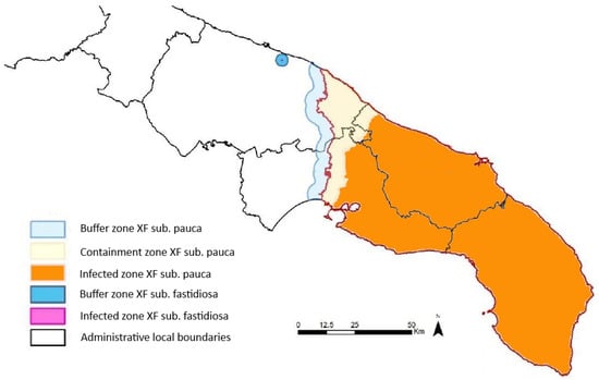
Figure 1.
Map of the infected zone, the containment zone, and the buffer zone in Apulia region, adapted from [13], depicting the situation in March 2024. The buffer, containment, and infected zones concerning the Xf subspecies pauca are, respectively, depicted in cyan, yellow, and orange. The small blue circle and the fuchsia centre represent buffer and infected zones concerning another Xf subspecies (not considered in this study).
However, recent advancements in remote sensing technology offer a promising alternative for the early detection and monitoring of Xf infection [17,18,19]. In 2018, for the first time to our knowledge, Zarco-Tejada et al. [17] demonstrated that it is possible to detect early Xf infection in olive groves by considering information extracted from hyperspectral and thermal data acquired by sensors on aircraft platforms. Their analysis is based on a data set composed of more than 7000 olive trees located in 15 groves in the Xf-infected area of the Apulia region (see Figure 1) and collected in 2016 and 2017. These data were labelled as “asymptomatic” or “symptomatic” trees (with four different stages of disease severity; see [17] for further details) by visual inspection. Only 100 trees from eight fields were also analysed by quantitative Polymerase Chain Reaction (qPCR) [20], resulting in 42 samples being labelled as not infected and 58 as infected. Many interesting experimental results were obtained. First of all, with a suitable combination of information retrieved from hyperspectral and thermal data, an automatic classification of “asymptomatic” and “symptomatic” trees was performed by using a Support Vector Machine (SVM) algorithm with a Gaussian kernel, obtaining detection accuracies exceeding 80%. Moreover, the detection obtained by the SVM on the 58 trees that tested positive for Xf infection, assessed by qPCR in the laboratory, was evaluated. It is worth noting that, among these 58 trees, 44 were “symptomatic” and 14 “asymptomatic”. The SVM correctly classified the whole set of “symptomatic” trees and recognized them as infected in 13 out of 14 “asymptomatic” trees. Finally, after the first assessment of disease severity performed in June 2016, 1700 trees were reevaluated in October 2016, February 2017, June 2017, and July 2017. In particular, 818 trees among the “true negatives” (i.e., trees that were classified as “asymptomatic” and were actually “asymptomatic”) and 178 trees among the “false positives” (i.e., trees that were classified as “symptomatic” but were actually “asymptomatic”) were followed in time, finding that many of them had become “symptomatic” but at different rates: 78% of the 818 “asymptomatic” trees in June 2016 were found to be “symptomatic” at the last revisit time in July 2017, while 96% of the “false positive” trees in June 2016 were found to be “symptomatic” in July 2017. Considering all these results, it is possible to argue that hyperspectral and thermal remotely sensed data, together with machine learning techniques, can be a feasible tool to detect trees that are infected by Xf, even before the appearance of visual symptoms. On the basis of these experimental results, other studies have been conducted to assess the feasibility of a large-scale monitoring system exploiting remotely sensed data. For example, Poblete et al. [18] focused their attention on the limitations due to the use of hyperspectral and thermal imaging systems, which generate massive data volumes when vast areas are analysed, with consequent long processing times. Moreover, they emphasized that hyperspectral cameras require accurate calibration processing, and if a service based on UAVs is considered, hyperspectral sensors that are usable as a drone’s payload are not easily found commercially. By considering the same data set as in Zarco-Tejada et al. [17], Poblete et al. [18] evaluated the use of a limited set of spectral bands along with the Crop Water Stress Index (CWSI), calculated from thermal imagery, for the automatic detection of Xf. In this case, the SVM classification accuracy decreased slightly to around 74%, suggesting that large-scale monitoring of Xf-infected areas can still be effectively supported using airborne platforms that are equipped with multispectral and thermal cameras. Specifically, the authors recommended using a limited number of carefully selected spectral bands, such as those in the blue and thermal regions, which are the most sensitive to Xf symptoms in olive trees. Similarly, Hornero et al. [19] considered satellite-based remote sensing data, particularly utilizing data from platforms like Sentinel 2, as a viable solution for monitoring the spread of Xf over extensive regions. The Sentinel 2 satellite offers moderate-to-high spatial resolution in 13 spectral bands, with a revisit time of up to five days. This combination of spatial, spectral, and temporal resolutions enables frequent monitoring of vegetation health and disease dynamics over large areas. However, despite its potential, satellite-based monitoring faces some important challenges, particularly in open vegetation canopies like in olive groves. Mixed-pixel effects due to canopy–scene components such as soil, shadows, and understory pose difficulties in accurately interpreting satellite data. Additionally, the spectral resolution of current satellite sensors may not be sufficient to detect the subtle changes associated with Xf infection.
Both Poblete et al. [18] and Hornero et al. [19] mainly consider the task of building an operational service for performing automatic detection of Xf from remotely sensed imagery as a feature reduction problem, i.e., a problem of evaluating the possibility of using a limited number of spectral bands, which are generally acquired by many commercial sensors or by satellites. In our opinion, another important aspect needs to be considered, which is the reduction in the available labelled data that are used to train the machine learning algorithms. It is well known that collecting accurate ground truth data is a complex, time-consuming, and costly process [17,21], particularly when it involves in situ surveys conducted by experts with specialized equipment. In our case, this challenge is even more pronounced, as each tree in the training and test sets must be labelled using qPCR to determine whether it is “affected” or “not affected” by Xf. This is a far more rigorous approach compared to visual inspection, which only distinguishes between “symptomatic” and “asymptomatic” trees.
In [17], a data set with a relevant size was available, with trees belonging to three different olive cultivars (Ogliarola Salentina, Cellina di Nardò, and Leccino), located in 15 groves, characterized by highly variable planting densities and overall management. The large number of labelled trees and their diverse characteristics—both genetic and influenced by external factors like agricultural practices—ensure the data set’s robustness. Combined with a high-performance algorithm such as an SVM, long considered the state of the art in various applications [22], it achieved a high classification accuracy. The high number of labelled samples also allowed the authors to consider a reduced set of features in input to the classifier [18] instead of the large number of spectral bands that are acquired by the hyperspectral sensor, while still obtaining good performances in classification. However, more experimental tests are needed to build a reliable and useful operational system to automatically detect Xf from remotely sensed data on large areas.
In the present study, we address several experimental issues that are essential for developing an operational service. First, we consider the fact that the classifier must be trained each time, leading to the following key question: how many labelled examples are needed to achieve an accurate classifier? Or, equivalently, is the available data set sufficiently large to build reliable predictors?
Another critical aspect concerns the current distribution of infected trees. At the present stage, in the recently identified infected areas, the number of infected trees remains, fortunately, very low. From an algorithmic perspective, this results in highly unbalanced data sets, posing a significant challenge for the classification of the minority class. Therefore, we also seek to answer the following question: to what extent does the balance between healthy and infected samples impact classifier performance?
Finally, we examine a data set that includes trees from geographically distant areas to assess how variability in cultivars and agricultural practices influences the classification performance, particularly when using a reduced training data set.
2. Materials and Methods
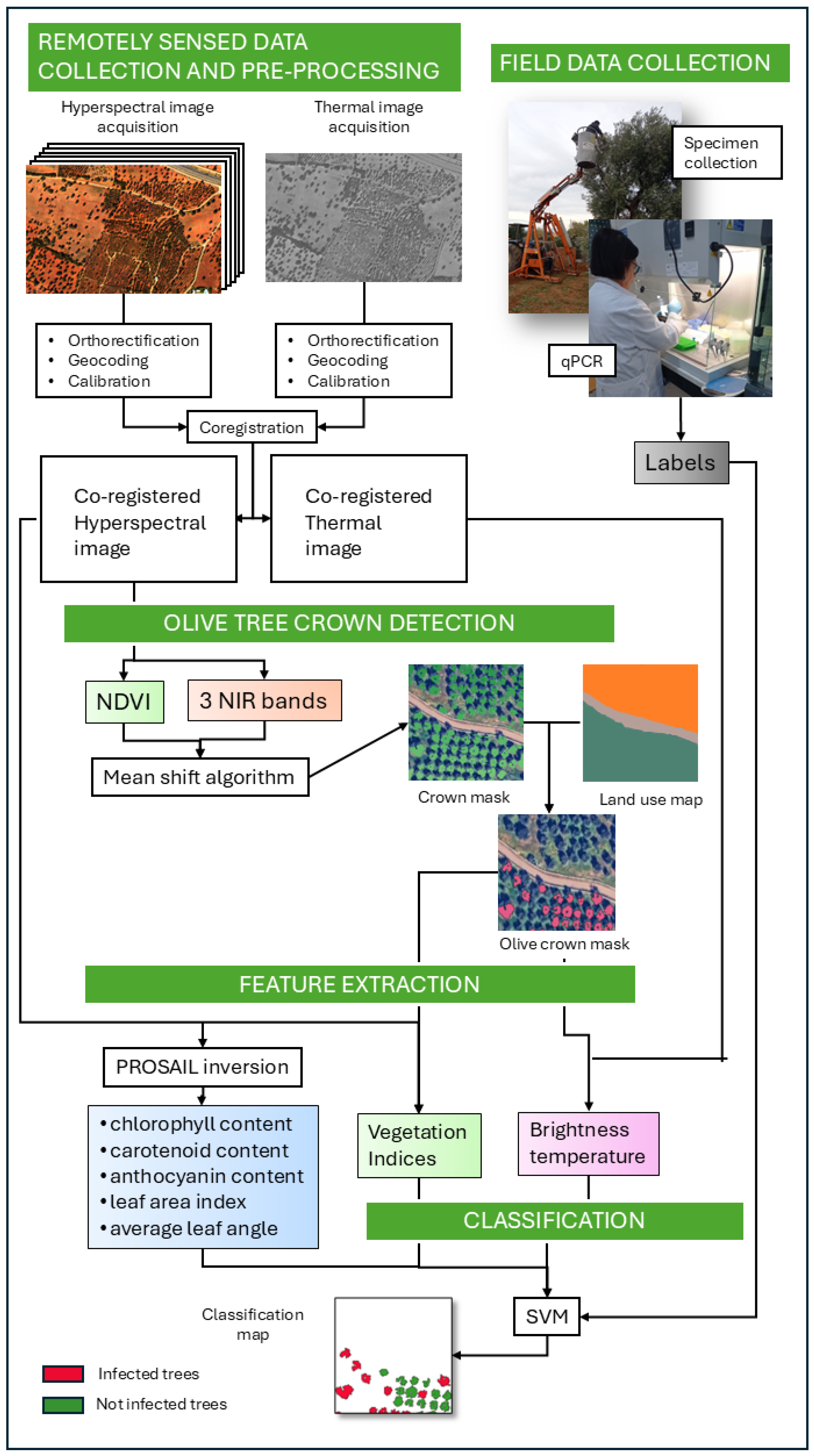
In this section, all the experimental steps that constitute the detection framework are presented. Moreover, to illustrate the complexity of the system more clearly, we provide a graphical schematic in Figure 2.

Figure 2.
Overview of the automated machine learning framework for Xf detection using hyperspectral and thermal imagery, together with field measurements. For details on each step in the figure, please see Section 2.
2.1. Field Data Collection
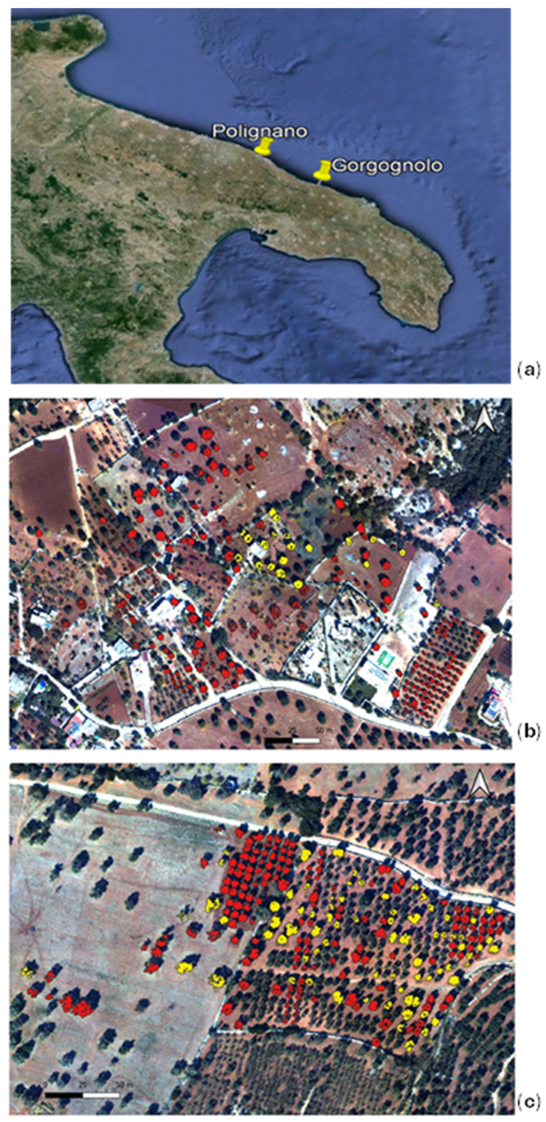
In September 2022, we assessed the presence of Xf in two contiguous olive groves located in the infected area of the Apulia region, Southern Italy, more precisely in the district of Gorgognolo (municipality of Ostuni, province of Brindisi), as depicted in Figure 3a. The field analysis consisted of the sampling of mature olive twigs. For symptomatic trees, twigs were gathered from branches exhibiting symptoms, while for asymptomatic trees, twigs were collected from the four cardinal points of the canopy, according to the official European and Mediterranean Plant Protection Organization (EPPO) guidelines [23]. Samples were automatically extracted with the Maxwell® RSC PureFood GMO and Authentication Kit and tested by qPCR [20] to verify the presence of the bacterium. In total, we evaluated 235 trees: 157 plants tested negative, and 78 tested positive for the Xf infection. The analysed olive trees were centuries old or relatively young (less than 50 years old), belonging to the cultivars Ogliarola Salentina, Cima di Melfi, and Leccino. Previous studies have proven that the first two cultivars are highly susceptible to Xf infection, while Leccino has genetic traits of resistance [24]. In fact, only 1 out of the 51 sampled Leccino trees tested positive. This first data set is identified in the following as the “Gorgognolo” data set and is depicted in Figure 3b.
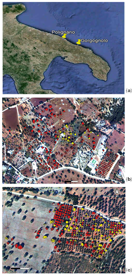
Figure 3.
(a) The location of the “Gorgognolo” area and “Polignano” area in the Apulia region; the RGB composition of three bands of the hyperspectral images acquired in the areas (b) of Gorgognolo and (c) Polignano in September 2022. The three bands are as follows: R: 695 nm; G: 515 nm; and B:410 nm. A mask of “infected” (yellow) and “not infected” (red) tree crowns is overlapped with the RGB images to show the spatial distribution of the trees in each data set.
Moreover, the Apulian phytosanitary authority, which performs surveillance campaigns every year to monitor the spread of Xf in the regional territory, collected data on the status of 155,500 trees in the containment zone from June 2022 to the day of imagery acquisition. These data, freely available on the Apulia region website [16], were used in the present work. They were tested and labelled using the procedure described in [7]. In particular, we considered an area in which, between 28 August 2022 and 28 September 2022, 20 infected trees were detected. This second experimental data set, named “Polignano”, which consists of the mentioned 20 infected trees (belonging to the Ogliarola cultivar), together with another 215 negative trees (tested with qPCR in the period of 26 August–17 October), is located in the same groves of the infected trees or in their neighbourhood, as reported in Figure 3c. For 100 trees in the not infected group, the cultivar is not specified, while the remainder belong to the Leccino (28 trees) and Ogliarola Barese (87 trees) cultivars.
2.2. Remotely Sensed Data Collection and Processing
On 22 September 2022, we captured imagery spanning 1.7 hectares within the Xf-infected and containment zones, as delimited by local authorities at the time of acquisition [12]. The Gorgognolo and Polignano areas, where the ground data were collected as described in the previous section, were included in the images acquired in the infected zone and in the containment one, respectively.
A hyperspectral sensor and a thermal camera mounted onboard a manned aircraft were used to acquire the imagery data. Flight parameters (altitude and airspeed) were chosen to obtain a final geometric resolution of 50 × 50 cm2 for both sensors.
The visible and near-infrared (NIR) regions were covered by a VNIR hyperspectral imager (CASI 1500, by ITRES Research Ltd., Calgary, Alberta, Canada) [25]. This is a pushbroom sensor that is capable of acquiring up to 288 bands between 350 and 1050 nm. However, as the number of bands increases, so does the Integration Time (IT) that is required for the sensor to record the signal of an entire line. This parameter affects the along-track spatial resolution, as the latter is directly proportional to the aircraft’s speed and the IT. For this reason, in order to achieve pixels of a 50 cm × 50 cm size, it was decided to operate with a reduced number of bands. The number of bands, as well as their individual positions and widths, was decided by taking into account and optimizing the information that was to be extracted from the hyperspectral images in terms of vegetation indices and other plant parameters, as reported in the literature [17,18]. Table 1 lists the 47 chosen bands, with the central wavelengths and the corresponding bandwidths. Orthorectification of the hyperspectral imagery was performed using the RCX (version 12.3) and GCSS (version 1.5) software suites, with inputs from an inertial measuring unit (Applanix FCS AV V5) that was synchronized with the hyperspectral imager. The conversion of radiance values, acquired by the sensor, to reflectance, was performed by using the empirical line method [26], based on hyperspectral measurements performed on the ground of selected targets and collected on different materials the same day of the aerial acquisitions, using an ASD FieldSpec Pro portable spectroradiometer (Analytical Spectral Devices, Inc. 2013, Malvern, UK).

Table 1.
List of CASI-1500 bands (CH), with their respective central wavelength (λ) and bandwidth (BW).
The thermal images were acquired by a broadband micro-TIR imager (MICRO TABI 640, ITRES Research Ltd., Calgary, AB, Canada) [27], with a broadband spectral response in the range of 3.7–4.8 μm and an across-track number of pixels of 640 and a Dynamic Range of 14 bits. For this second sensor, calibration procedures were also performed in the ITRES laboratories before the flight. Using the previously mentioned RCX and GCSS software, the raw thermal data were converted to brightness temperature images according to Planck’s law. Land Surface Temperature conversion was not deemed necessary, as in our analysis, only tree crown pixels were considered, for which it can be safely assumed that the emissivity is constant, with a value very close to 1 [28]. Orthorectification of the thermal imagery was performed in the same way as with the CASI-1500 images. The thermal and hyperspectral images were also precisely co-registered.
2.3. Feature Extraction
From each hyperspectral image, we identified individual trees using automatic object-based crown detection algorithms. For our analysis, we employed a segmentation technique based on the Mean-Shift clustering algorithm [29] applied to a combination of a masked-by-threshold NDVI and the three infrared bands. We also imposed a minimum and maximum area for segments to more effectively detect tree crowns. Each resulting segment is a set of fully connected pixels that have been assigned a different identification number and are used for further analysis. The olive tree crowns were detected by intersecting the whole set of segments with a land use map of the Apulia Region, reporting, for each crop field, its cultivation.
From each tree crown, the mean reflectance value in each spectral band and the mean temperature value were extracted. Following Zarco-Tejada et al. [17], from the 47 spectral bands, we computed 56 vegetation indices associated with chlorophyll, carotene, and xanthophyll pigments, which are subject to physiological changes in response to the pathogen. The indices are listed in Table 2. Moreover, still in accordance with Zarco-Tejada et al. [17], we computed some canopy structural parameters and leaf biochemical constituents that we obtained by the inversion of the PROSAIL radiative transfer model, using data from pure vegetation pixels extracted from each tree crown. PROSAIL is a well-known radiative transfer model [30], which integrates the PROSPECT leaf reflectance model, which simulates reflectance spectra from leaf properties like pigment concentrations, and the SAIL canopy reflectance model, accounting for the canopy’s structural properties such as the leaf inclination and sun-observer geometry. Specifically, we utilized the PROSPECT-D and 4SAIL versions for this study. The inversion process of PROSAIL utilized a look-up-table (LUT) approach, with most parameters being kept at fixed values and only five, namely chlorophyll content, carotenoid content, anthocyanin content, leaf area index (LAI), and average leaf angle, being varied within sets of discrete values in a defined range. The discrete values and the ranges of variability of the model parameters were the same as those used by Zarco-Tejada et al. [17]. The correspondence between the simulated spectra and airborne spectra was assessed using the root mean square error (RMSE). Trait estimates were obtained by selecting the top 1% of LUT entries with the lowest RMSE values and then computing a weighted average of the corresponding parameter values, with weights being assigned as the inverse of their RMSE.
Table 2.
List of vegetation indices (VIs) and corresponding equations.
Thus, in summary, for each tree, a vector composed of 62 features was considered: the 56 vegetation indices in Table 2, the thermal value, and the above-mentioned 5 biological and structural parameters, obtained through the inversion of the PROSAIL model.
2.4. Online Available Data
The freely available data set published by Zarco-Tejada et al. [17] was initially considered for comparison and analysis. As described in Section 1, it is composed of an array of 76 features, collected from 7296 olive trees, of which 4045 are labelled as “asymptomatic” and 3251 as “symptomatic”. It is worth noting again that in this data set, the samples were labelled by visual inspection, which justifies the labelling of “asymptomatic/symptomatic” instead of “infected/not infected”, which we use for our data. To train/test our classifier with these data and compare the results, the subset of 62 features listed in the previous section was extracted from the 76.
2.5. Automatic Classification Algorithms
Information retrieved from the hyperspectral and thermal imagery was classified using an SVM [31] to automatically detect trees that were infected by Xf. An SVM is a flexible learning model encompassing polynomial classifiers, neural networks, and RBF networks within its scope. In the field of two-class pattern recognition, the SVM’s methodology involves mapping data into a higher-dimensional feature space with respect to the original one. Moreover, the minimization of an upper bound of the structural risk, composed of the empirical risk term and a penalty term depending on the complexity of the classifier used, instead of the minimization of the empirical one alone, allows for a high generalization capability (see [32] and definitions therein).
2.6. Evaluation Metrics
The metrics used to assess the classifier performance are the overall accuracy (OA), the F-score (FP) computed with respect to the positive class of “infected” trees, and the Recall Rate (Re). In particular,
where TN is the number of true negatives, i.e., trees labelled as “not infected” and classified as “not infected”, TP is the number of True Positives, i.e., trees labelled as “infected” and classified as “infected”, FN is the number of False Negatives, i.e., trees labelled as “infected” and classified as “not infected”, and FP is the number of false positives, i.e., trees labelled as “not infected” and classified as “infected”. In the following, the OA, the FP, and the Re values are expressed as percentages.
In particular, the FP metric is considered, because significant attention is paid to the positive class, and one given value of OA may correspond to several values of FP and to very different performances of classifiers. For example, let us consider a test set composed of 100 samples, equally divided into two classes. An OA = 80% (i.e., 80 samples being correctly classified out of 100) can be obtained when the whole set of 50 negative samples are correctly classified together with 30 out of 50 positives (FP = 75%), but also, e.g., in the opposite case when the whole set of positive samples are correctly classified together with 30 out of the 50 negatives (FP = 83%).
Moreover, given that Xf is a highly destructive plant pathogen, the Re metric supplies useful information about the missed detection of infected trees (FN), which is a crucial aspect to consider in this particular application.
3. Results
3.1. Analysis of Training Set Dimension
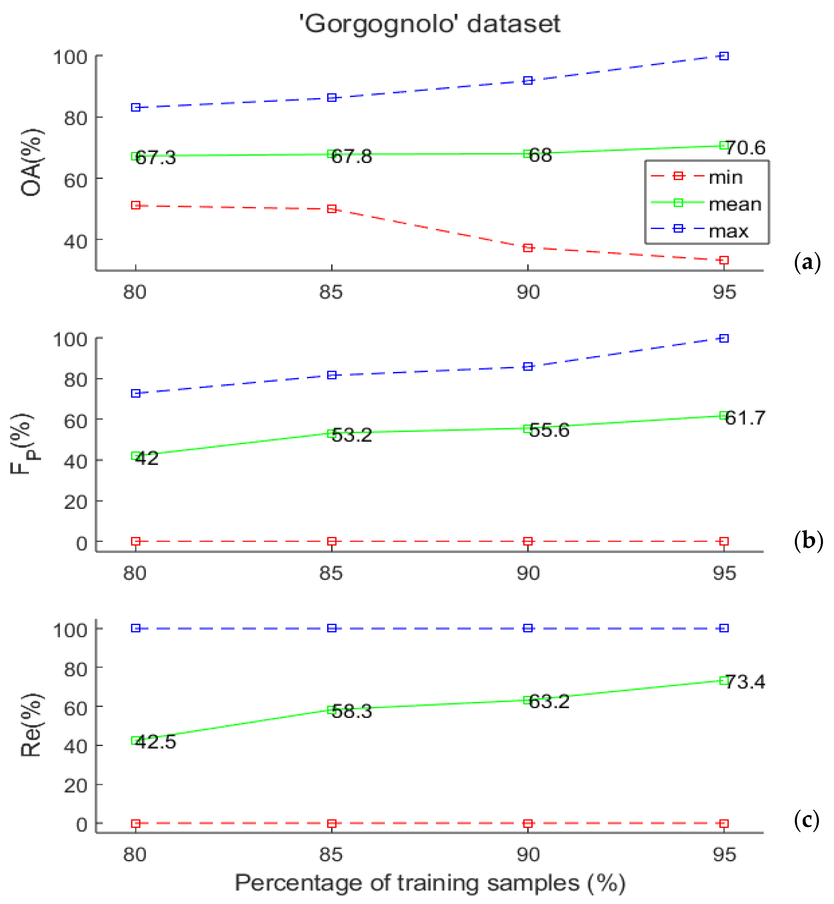
We assessed the generalization capability of the SVM classifier, evaluated through the Leave-K-Out cross-validation method, by varying the number of training examples to understand if the available data set size is sufficient to obtain good performances of the considered classifier. To achieve this goal, for each considered training set size, we considered 500 random training/test splits of the data while maintaining the same proportion of positive and negative examples in the entire data set. Specifically, we considered training data sets comprising 80%, 85%, 90%, and 95% of the labelled data. As stated in Section 2.1, the “Gorgognolo” data set is composed of 235 labelled samples, so the numbers of data points that are used to train the SVM algorithm in the various cases are, respectively, equal to 188, 199, 211, and 223.
It is worth noting that the “Gorgognolo” data set is slightly unbalanced, as the number of negative trees is twice that of positives. For this reason, we set the misclassification cost of the minority class to equal 2. This is a weight that is applied to the minority class outcomes to specify that errors on the minority examples are more costly than the ones on the other class. The experimental results are depicted in Figure 4a,b, in which the value ranges of the above-mentioned evaluation metrics are reported. Some considerations are in order. First of all, the minimum FP in panel (b) and the minimum Re in panel (c) are constantly zero, because in all cases, some of the splits gave no positive classified samples in the test. This happened for 24 cases out of 500 when we used 80% of the data in training, once when 85% and 90% of samples were used in training, and twice when 95% was considered. For all the metrics, the mean values increased with the training set dimension; however, the obtained results became more variable (the statistical range increased, as shown in the figures), because the dimension of the test set was drastically reduced. As pointed out in [33], such evidence seems counter-intuitive when considering that it was obtained using the maximum training set size, but it becomes immediately evident when we consider the test set size and, in particular, when the Leave-One-Out (LOO) error procedure is examined. In the LOO error procedure, the test set consists of a single example, making the likelihood that a random classifier can correctly classify the test example by chance relatively high. However, as the test set size increases, this likelihood decreases.
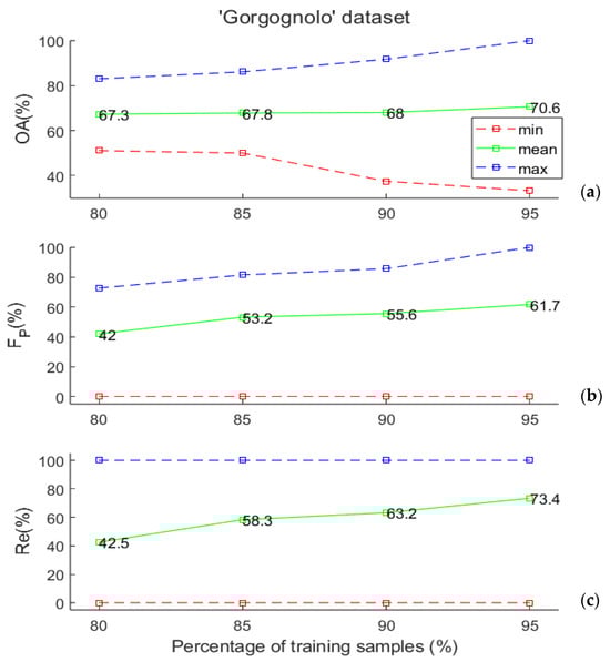
Figure 4.
(a) Overall accuracy, (b) FP, and (c) Re values (minimum, mean, and maximum over 500 random data set splits) as a function of the training set size for the “Gorgognolo” data set. All values are computed on the test set.
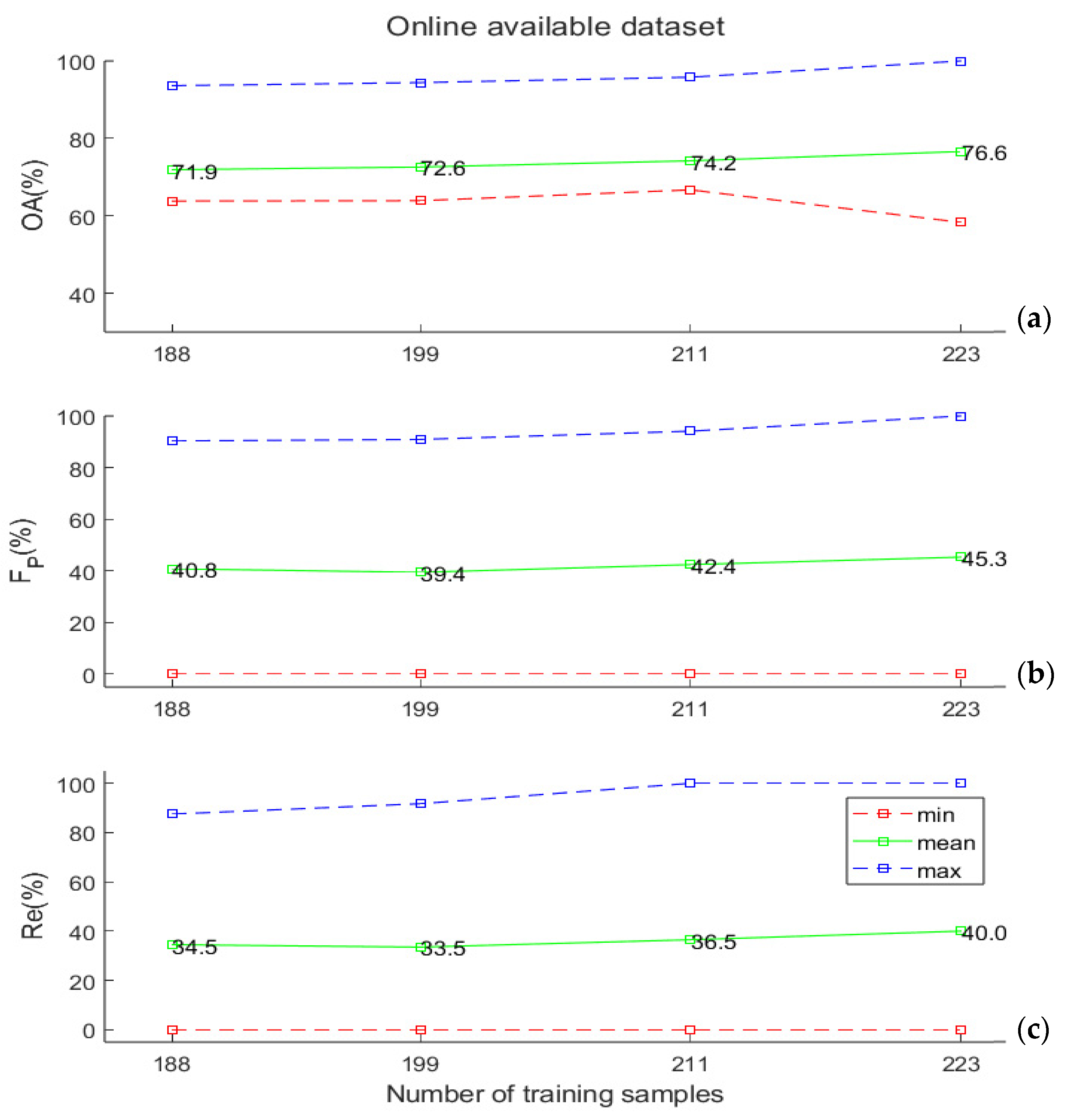
In Figure 5a,b, the experimental results obtained by applying the SVM classifier to the online data set described in Section 2.4 are illustrated. In this benchmark experiment, we tested the classification performance by artificially reducing the size of the training/test data sets. In particular, we performed 500 extractions of 235 data points each from the original data set. We repeated the procedure 4 times, each time dividing each of the 235-samples dataset by different percentages (from 80%–20% to 95%–5%) among the training and test. The OA values were, in this case, slightly better than the ones obtained on the “Gorgognolo” data, but the capability to efficiently detect symptomatic trees, as expressed by the FP and Re values, was highly reduced here.
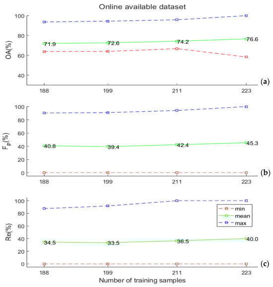
Figure 5.
(a) Overall accuracy values, (b) FP values, and (c) Re values (minimum, mean, and maximum), obtained by varying the training set size that was computed based on the online data set described in Section 2.4. All these values were computed on the test set. Here, the abscissa reports the absolute number of training samples extracted randomly from the data set, which coincide with the numbers in the “Gorgognolo” data set (Figure 4), corresponding to the same fractions (80%, 85%, 90%, and 95%) of all the labelled samples in our data.
The same analysis was conducted on the “Polignano” data set, which is, however, severely unbalanced. For this reason, we set the misclassification cost of the minority class as equal to 10. This was a very interesting test, because it gave us many suggestions on the impact of an unbalanced data set on the classification results. First of all, we only considered training data sets consisting of 80% and 85% of the labelled data, which present, respectively, only four and three positive samples in the test set. The other two cases were not taken into account, as the number of samples in the minority class were too small. Actually, these experimental results could appear to be better than the ones obtained on the “Gorgognolo” data set in terms of the mean values of the indices, but we have to consider that, for instance, when all the examples were classified as negative (i.e., FP = 0), which represents a trivial outcome, the corresponding OA was equal to 91.5%. This occurred 203 times out of the 500 when we considered 85% of the data in training. Moreover, the mean OA equalled 92.8%.
3.2. Spatial Analysis
In agreement with Zarco-Tejada’s approach [17], we considered the best classifiers that we obtained for each training data set size. The performances of these classifiers are reported in Table 3. We also tested them on the “Polignano” data set to understand how they perform on another geographical area. Each considered classifier correctly recognized as positive only 2 trees out of the 20 labelled as positive in the ground data (OA = 92.3%; FP = 18.2%; Re = 10%).
Table 3.
Performances of the best classifiers obtained for each training data set size for the “Gorgognolo” data set. In the last column on the right is the number of classifiers out of 500, showing the performance in the second column. For the training set size equal to 85%, the FP values corresponding to the two experiments that both led to the maximum OA of 86.1% are reported.
3.3. Joint Data Set Analysis
Finally, we considered a joint data set, composed of data belonging to both the “Gorgognolo” and the “Polignano” areas. In order to properly compare the experimental results, we considered 235 samples out of the 470 that were available in total. The partition between the training and test set was fixed to 85% in training and 15% in test. Two different compositions of the data sets were taken into account: the first one (data set 1) has the same proportion of positive and negative data collected in the two geographical areas, both in training and test; in the second one (data set 2), the number of positive samples from the “Polignano” data set is maximized in training, while the negative samples are extracted in the same proportions from the two areas. For clarity, the data sets’ compositions are reported in Table 4. Here again, 500 random extractions of 235 samples from the whole set of 470 data points were performed for each of the considered data sets.
Table 4.
Compositions of the training and test data sets, obtained by joining the data collected in the “Gorgognolo” and “Polignano” areas.
For both data sets, the misclassification cost of the minority class was set as equal to 2. For data set 1, the mean OA value was equal to 68.3%, comparable with the mean value (67.8%) obtained for the same training size when only the labelled data of the “Gorgognolo” area were considered (see Figure 4). The mean FP value was equal to 45.2%, lower than the corresponding value (FP = 53.2%) obtained with the “Gorgognolo” data. The mean Re value was equal to 46.0%, which was also in this case lower than the corresponding value (Re = 58.3%) obtained with the “Gorgognolo” data. Conversely, for data set 2, the mean values of OA, FP, and Re equalled 74.1%, 55.8%, and 54.6%, respectively. The first two metrics were consistently better than the corresponding ones obtained on the “Gorgognolo” data. For the Re metric, it is important to highlight that the number of positives in the test set is in both data sets (“Gorgognolo” and “Gorgognolo”+”Polignano” data set 2) equalled 12, and the difference between the two mean values did not correspond to a difference in the number of positives that were correctly recognized (i.e., 7 out of 12).
4. Discussion
Some considerations are in order. First of all, the size of the experimental data set is certainly a key point in obtaining good classification performances, together with its balance with respect to the two classes and its representativeness of the different cultivars and agricultural practices that are present in a wide region.
The results obtained from the data set consisting of only 235 labelled samples, collected from a single area (the “Gorgognolo” data set), align with those from the reference online data set, appropriately reduced for comparison. The OA values are lower, probably due to differences in the representativeness of the two data sets. As previously mentioned, the “Gorgognolo” data set includes trees from three different cultivars (Ogliarola Salentina, Cima di Melfi, and Leccino), located in two neighbouring groves. The online data set also encompasses trees from three cultivars (Ogliarola Salentina, Cellina di Nardò, and Leccino) but is distributed across 15 groves with different planting densities and diverse management practices. Notably, when we consider a data set including trees from two distinct areas (“Gorgognolo” and “Polignano”), which are geographically distant and characterized by different agricultural practices, the results on our data outperform those obtained using the online data set (see Figure 5). Summarizing these results, we conclude that even a reduced data set of, e.g., as few as 200 samples (see Table 4), can be effective for building a robust classifier. However, it is essential that the sampled trees come from different geographical areas and belong to different cultivars to capture as much of the variability that is present within the analysed data as possible.
In fact, when the classifier had been trained only with the “Gorgognolo” data set, the test performed on the “Polignano” data showed a low rate of recognition for the infected trees, i.e., a poor ability to be usefully applied in geographical areas that are distant from the one of the training set. In more detail, the infected trees in the “Polignano” data set belong to the Ogliarola barese cultivar, which is not represented in the “Gorgognolo” training set; this factor could be relevant for the missed recognitions. Moreover, in this geographical area, the management of olive groves is considerably different to that of the Gorgognolo zone in terms of agricultural practices such as irrigation, pruning, or weed control.
Another key point concerns the balance of the data set. The “Polignano” data set is highly unbalanced (only 8.5% of the labelled data are marked as “infected”), and the experimental results obtained on this data set do not allow for the construction of a robust classifier. Certainly, there are other machine learning techniques in the literature that are more suitable to classify severely unbalanced data sets, such as the RUSBoost algorithm [34], which has also been successfully applied to the analysis of hyperspectral and thermal data for the automatic detection of trees that are infected by Xylella fastidiosa [35]. However, exploring alternative classifiers is beyond the scope of this work. Instead, our focus is on identifying the optimal characteristics of a data set that can be collected to build an SVM classifier with high classification performance.
For this reason, we analysed the two different compositions of the joint data set. The best experimental results were obtained with data set 2. In this case, the data labelled as negative in the training set were balanced with respect to their geographical origin. Instead, in the positive class, where a balanced condition was numerically impossible to achieve, the whole set of positive samples from the “Polignano” data set (17 in training, 3 in test) was used in order to be as close as possible to a balanced data set with respect to the geographical origin of the data. This point represents a serious challenge, because it implies that in an operational context, significant attention should be paid to the selection of areas for the sampling of the training set based on a deep knowledge of the territory characteristics and previous information about the spread of Xf infection in it.
It is also important to point out that all the issues analysed in this study are based on the goal of developing an operational system for the detection of Xf. This work builds on key findings from the literature [17,18,19] and aims to address some existing gaps in establishing a system that can be used effectively across a large area. Many experimental choices, including the selection of the classifier algorithm, were made with this objective in mind. For future work, additional classifiers—such as random forests [36], which have demonstrated superior performance compared to SVMs in other application domains—will be tested on our data. Another important direction for future research is the application of data augmentation methods. This presents a significant challenge, because, to our knowledge, there are only a few documented cases of data augmentation techniques being applied to spectral data [37] and none involving remotely acquired spectral data.
Moreover, the present study is only based on data acquired in September 2022. The next step in our analysis will be to consider a multi-temporal data set to assess the robustness of the classifier when tested on data acquired in the same area but at different times. Additionally, we will evaluate whether enriching the labelled training set is necessary to achieve better performance.
Finally, the present analysis focuses on the Apulia region, which is characterized by significant variability in olive cultivars and agricultural practices. However, it would be interesting to test this experimental framework in other geographical areas with different climate conditions. Based on the current experimental results, it is reasonable to assume that retraining will be necessary to capture as much variability as possible in the new data.
5. Conclusions
In this paper, we explored the performance of an automatic procedure based on an SVM-supervised classifier for the detection of olive trees that are infected by the Xylella fastidiosa bacterium from airborne high-resolution hyperspectral and thermal image data. The procedure includes the pre-processing of the remotely sensed data, extraction of tree crown pixels through image segmentation, and computation of relevant indices from hyperspectral reflectance values, as well as other indicators obtained from the inversion of radiative transfer models, for a total of 62 features. The training and testing of the classifier were based on data collected through qPCR analyses of leaves and twigs, sampled on the ground from affected and not affected olive trees. The results obtained for a test site in the Apulia region (southern Italy), where the infection is currently spreading, were analysed, with particular attention to the issues of sample size and balance. The experiment, whose outcomes were also compared to benchmark experiments conducted on samples of a similar size extracted from data sets in the literature, offers insights into several important questions which may arise when setting up an automated detection service for application to large areas. The results show that the SVM-supervised classifier can be effectively trained with as few as 200 labelled data points, even when they are slightly unbalanced between the two classes of interest of “infected” and “not infected” trees, to obtain acceptable results, with overall accuracies above 74%.
These results demonstrate that an operational system for automatically detecting new Xf outbreaks in olive groves using remotely sensed data could provide valuable support to the sampling methods currently in use. However, to develop an efficient system for broader applications, it is essential to gather training data from multiple groves across different geographical areas. This approach is necessary to capture the significant variability in cultivars and agricultural practices across a large territory.
Author Contributions
Conceptualization and methodology, A.D.; software, A.D., F.L. and A.R.; validation, A.D., F.L. and A.R.; formal analysis, A.D., F.L., A.R. and A.B.; investigation, A.D., R.M., F.L., A.R., A.B., F.B., A.G., S.S.A., R.A.K., G.M. and D.B.; resources, A.D., R.M., G.M. and D.B.; data curation, A.D., R.M. and F.L.; writing—original draft preparation, A.D.; writing—review and editing, all authors; visualization, A.D. and A.R.; supervision, A.D., R.M., G.M. and D.B. All authors have read and agreed to the published version of the manuscript.
Funding
This research was funded by the Italian Business and Made in Italy Ministry (MIMIT), under the framework of the “Remote Early Detection of Xylella” (REDoX) project, Prog. n. F/200139/01-03/X45.
Acknowledgments
The authors thank M. Mottola (CNR-IREA) for her support in the administrative management of the REDoX project.
Conflicts of Interest
The authors declare no conflicts of interest.
References
- EFSA Panel on Plant Health (PLH); Bragard, C.; Dehnen-Schmutz, K.; Di Serio, F.; Gonthier, P.; Jacques, M.-A.; Jaques Miret, J.A.; Justesen, A.F.; MacLeod, A.; Magnusson, C.S.; et al. Update of the Scientific Opinion on the risks to plant health posed by Xylella fastidiosa in the EU territory. EFSA J. 2019, 17, 5665. [Google Scholar] [CrossRef]
- EFSA (European Food Safety Authority); Cavalieri, V.; Fasanelli, E.; Gibin, D.; Gutierrez Linares, A.; La Notte, P.; Pasinato, L.; Delbianco, A. Update of the Xylella spp. host plant database—Systematic literature search up to 31 December 2023. EFSA J. 2024, 22, e8898. [Google Scholar] [CrossRef] [PubMed]
- Sicard, A.; Zeilinger, A.R.; Vanhove, M.; Schartel, T.E.; Beal, D.J.; Daugherty, M.P.; Almeida, R.P.P. Xylella fastidiosa: Insights into an Emerging Plant Pathogen. Annu. Rev. Phytopathol. 2018, 25, 181–202. [Google Scholar] [CrossRef]
- Sicard, A.; Saponari, M.; Vanhove, M.; Castillo, A.I.; Giampetruzzi, A.; Loconsole, G.; Saldarelli, P.; Boscia, D.; Neema, C.; Almeida, R.P.P. Introduction and adaptation of an emerging pathogen to olive trees in Italy. Microb. Genom. 2021, 7, 000735. [Google Scholar] [CrossRef] [PubMed]
- Saponari, M.; Boscia, D.; Altamura, G.; Loconsole, G.; Zicca, S.; D’Attoma, G.; Morelli, M.; Palmisano, F.; Saponari, A.; Tavano, D.; et al. Isolation and pathogenicity of Xylella fastidiosa associated to the olive quick decline syndrome in southern Italy. Sci. Rep. 2017, 7, 17723. [Google Scholar] [CrossRef]
- Saponari, M.; Boscia, D.; Nigro, F.; Martelli, G.P. Identification of DNA Sequences Related to Xylella fastidiosa in Oleander, Almond And Olive Trees Exhibiting Leaf Scorch Symptoms In Apulia (Southern Italy). J. Plant Pathol. 2013, 95, 668. [Google Scholar]
- Kottelenberg, D.; Hemerik, L.; Saponari, M.; van der Werf, W. Shape and rate of movement of the invasion front of Xylella fastidiosa spp. pauca in Puglia. Sci. Rep. 2021, 11, 1061. [Google Scholar] [CrossRef]
- EPPO. First Report of Xylella fastidiosa in Israel. EPPO Reporting Service No. 6, Global Database. 2019. Available online: https://gd.eppo.int/reporting/article-6551 (accessed on 14 January 2025).
- Amanifar, N.; Taghavi, M.; Izadpanah, K.; Babeik, G. Isolation and pathogenicity of Xylella fastidiosa from grapevine and almond in Iran. Phytopathol. Mediterr. 2014, 53, 318–327. [Google Scholar] [CrossRef]
- European Union. Commission Implementing Decision (EU) 2015/789 of 18 May 2015 as Regards Measures to Prevent the IntrodDuction into and the Spread Within the Union of Xylella fastidiosa (Wells et al.). Available online: https://eur-lex.europa.eu/eli/dec_impl/2015/789/oj (accessed on 14 January 2025).
- European Union. Commission Implementing Regulation (EU) 2020/1201 of 14 August 2020 as Regards Measures to Prevent the Introduction into and the Spread Within the Union of Xylella fastidiosa (Wells et al.). Available online: https://eur-lex.europa.eu/legal-content/EN/TXT/?uri=CELEX%3A32020R1201 (accessed on 14 January 2025).
- European Union. Commission Implementing Regulation (EU) 2024/1320 of 15 May 2024 Amending Implementing Regulation (EU) 2020/1201 as Regards the List of Infected Zones for Containment of Xylella fastidiosa (Wells et al.). Available online: https://eur-lex.europa.eu/legal-content/EN/TXT/?uri=OJ:L_202401320 (accessed on 14 January 2025).
- Apulia Region Report n. 18/2024, 2024. Last Update of Delimitated Zones for Xylella fastidiosa subspecies Pauca. Available online: https://burp.regione.puglia.it/documents/20135/2470544/DET_48_3_5_2024.pdf (accessed on 14 January 2025).
- EFSA (European Food Safety Authority); Lázaro, E.; Parnell, S.; Vicent Civera, A.; Schans, J.; Schenk, M.; Schrader, G.; CortiñasAbrahantes, J.; Zancanaro, G.; Vos, S. Guidelines for Statistically Sound and Risk-Based Surveys of Xylella fastidiosa; EN-1873; EFSA Supporting Publication: Parma, Italy, 2020; 76p. [Google Scholar] [CrossRef]
- Action Plan to Prevent the Spread of Xylella fastidiosa (Well et al.) in Puglia—Three-Year Period 2024–2026. Available online: https://burp.regione.puglia.it/documents/20135/2560952/DEL_1593_2024.pdf/4501bf7f-c5ec-face-57d4-a559581af1c2?t=1733751415831 (accessed on 14 January 2025).
- Available online: http://www.emergenzaxylella.it/portal/portale_gestione_agricoltura/ (accessed on 14 January 2025).
- Zarco-Tejada, P.J.; Camino, C.; Beck, P.S.A.A.; Calderon, R.; Hornero, A.; Hernandez-Clemente, R.; Kattenborn, T.; Montes-Borrego, M.; Susca, L.; Morelli, M.; et al. Previsual symptoms of Xylella fastidiosa infection revealed in spectral plant trait alterations. Nat. Plants 2018, 4, 432–439. [Google Scholar] [CrossRef]
- Poblete, T.; Camino, C.; Beck, P.S.A.; Hornero, A.; Kattenborn, T.; Saponari, M.; Boscia, D.; Navas-Cortes, J.A.; Zarco-Tejada, P.J. Detection of Xylella fastidiosa infection symptoms with airborne multispectral and thermal imagery: Assessing bandset reduction performance from hyperspectral analysis. ISPRS J. Photogramm. Remote Sens. 2020, 162, 27–40. [Google Scholar] [CrossRef]
- Hornero, A.; Hernández-Clemente, R.; North, P.R.J.; Beck, P.S.A.; Boscia, D.; Navas- Cortes, J.A.; Zarco-Tejada, P.J. Monitoring Xylella fastidiosa infection symptoms in olive orchards using Sentinel 2 imagery and 3-D radiative transfer modelling. Remote Sens. Environ. 2020, 236, 111480. [Google Scholar] [CrossRef]
- Harper, S.J.; Ward, L.I.; Clover, G.R.G. Development of LAMP and Real-Time PCR Methods for the Rapid Detection of Xylella fastidiosa for Quarantine and Field Applications. Phytopathology 2010, 100, 1282–1288. [Google Scholar] [CrossRef] [PubMed]
- Bovolo, F.; Bruzzone, L. The Time Variable in Data Fusion: A Change Detection Perspective. IEEE Geosci. Remote Sens. Mag. 2015, 3, 8–26. [Google Scholar] [CrossRef]
- Fernandez-Delgado, M.; Cernadas, E.; Barro, S.; Amorim, D. Do we Need Hundreds of Classifiers to Solve Real World Classification Problems? J. Mach. Learn. Res. 2014, 15, 3133–3181. Available online: https://jmlr.org/papers/volume15/delgado14a/delgado14a.pdf (accessed on 14 January 2025).
- EPPO. PM 7/24 (4) Xylella fastidiosa. EPPO Bull. 2019, 49, 175–227. [Google Scholar] [CrossRef]
- Giampetruzzi, A.; Morelli, M.; Saponari, M.; Loconsole, G.; Chiumenti, M.; Boscia, D.; Savino, V.N.; Martelli, G.P.; Saldarelli, P. Transcriptome profiling of two olive cultivars in response to infection by the CoDiRO strain of Xylella fastidiosa subsp. pauca. BMC Genom. 2016, 17, 475. [Google Scholar] [CrossRef]
- Available online: http://www.gstdubai.com/downloads/CASI-1500.pdf (accessed on 14 January 2025).
- Ortiz, J.D.; Avouris, D.; Schiller, S.; Luvall, J.C.; Lekki, J.D.; Tokars, R.P.; Anderson, R.C.; Shuchman, R.; Sayers, M.; Becker, R. Intercomparison of approaches to the empirical line method for vicarious hyperspectral reflectance calibration. Front. Mar. Sci. 2017, 4, 296. [Google Scholar] [CrossRef]
- Available online: https://www.itres.com/wp-content/uploads/2024/06/microTABI-640-Specification-Sheet-06.2024.pdf (accessed on 14 January 2025).
- Merchant, C.J. Thermal Infrared Remote Sensing; Kuenzer, C., Dech, S., Eds.; Remote Sensing and Digital Image Processing; Springer: Dordrecht, The Netherlands, 2013; Volume 17, ISBN 978-94-007-6638-9. [Google Scholar]
- Comaniciu, D.; Meer, P. Mean shift: A robust approach toward feature space analysis. IEEE Trans. Pattern Anal. Mach. Intell. 2002, 24, 603–619. [Google Scholar] [CrossRef]
- Jacquemoud, S.; Verhoef, W.; Baret, F.; Bacour, C.; Zarco-Tejada, P.J.; Asner, G.P.; François, C.; Ustin, S.L. PROSPECT+SAIL models: A review of use for vegetation characterization. Remote Sens. Environ. 2009, 113, S56–S66. [Google Scholar] [CrossRef]
- Vapnik, V. Statistical Learning Theory; John Wiley & Sons, Inc.: Hoboken, NJ, USA, 1998. [Google Scholar]
- Scholkopf, B.; Sung, K.; Burges, C.J.C.; Girosi, F.; Niyogi, P.; Poggio, T.; Vapnik, V. Comparing Support Vector Machines with Gaussian Kernels to Radial Basis Function Classifiers. IEEE Trans. Signal Process. 1997, 45, 2758–2765. [Google Scholar] [CrossRef]
- Ancona, N.; Maglietta, R.; Piepoli, A.; D’Addabbo, A.; Cotugno, R.; Pesole, G.; Liuni, S.; Savino, M.; Carella, M.; Perri, F. On the statistical assessment of classifiers using DNA microarray data. BMC Bioinform. 2006, 7, 387. [Google Scholar] [CrossRef] [PubMed]
- Seiffert, C.; Khoshgoftaar, T.M.; Van Hulse, J.; Napolitano, A. RUSBoost: A Hybrid Approach to Alleviating Class Imbalance. IEEE Trans. Syst. Man Cybern.—PART A Syst. Hum. 2010, 40, 185–197. [Google Scholar] [CrossRef]
- D’Addabbo, A.; Belmonte, A.; Bovenga, F.; Lovergine, F.; Refice, A.; Matarrese, R.; Gallo, A.; Mita, G.; Abou Kubaa, R.; Boscia, D.; et al. Automatic Detection of Xylella Fastidiosa in Aerial Hyperspectral and Thermal Data. In Proceedings of the 2023 IEEE International Geoscience and Remote Sensing Symposium (IGARSS 2023), Pasadena, CA, USA, 16–21 July 2023. [Google Scholar]
- Hastie, T.; Tibshirani, R.; Friedman, J. The Elements of Statistical Learning, 2nd ed.; Springer: Berlin/Heidelberg, Germany, 2008; ISBN 0-387-95284-5. [Google Scholar]
- Chung, J.; Zhang, J.; Saimon, A.I.; Liu, Y.; Johnson, B.N.; Kong, Z. Imbalanced spectral data analysis using data augmentation based on the generative adversarial network. Sci. Rep. 2024, 14, 13230. [Google Scholar] [CrossRef] [PubMed]

Disclaimer/Publisher’s Note: The statements, opinions and data contained in all publications are solely those of the individual author(s) and contributor(s) and not of MDPI and/or the editor(s). MDPI and/or the editor(s) disclaim responsibility for any injury to people or property resulting from any ideas, methods, instructions or products referred to in the content. |
© 2025 by the authors. Licensee MDPI, Basel, Switzerland. This article is an open access article distributed under the terms and conditions of the Creative Commons Attribution (CC BY) license (https://creativecommons.org/licenses/by/4.0/).