High-Precision Multi-Source Fusion Navigation Solutions for Complex and Dynamic Urban Environments

Abstract

With the rapid advancement of artificial intelligence, particularly in fields such as autonomous driving, drone delivery, and logistics automation, the demand for high-precision and robust navigation services has become critical. In complex and dynamic urban environments, the navigation capabilities of single-sensor systems struggle to meet the practical requirements of autonomous driving technology. To address this issue, we propose a multi-source fusion navigation algorithm tailored for dynamic urban canyon scenarios, aiming to achieve reliable and continuous state estimation in complex environments. In our proposed method, we utilize independent threads on a graphics processing unit (GPU) to perform real-time detection and removal of dynamic objects in visual images, thereby enhancing the visual accuracy of multi-source fusion navigation in dynamic scenes. To tackle the challenges of significant Global Navigation Satellite System (GNSS) positioning errors and limited satellite availability in urban canyon environments, we introduce a specialized GNSS Real-Time Kinematic (RTK) stochastic model for such settings. The navigation performance of the proposed algorithm was evaluated using public datasets. The results demonstrate that our RTK/INS/Vision integrated navigation algorithm effectively improves both accuracy and availability in dynamic urban canyon environments.

1. Introduction

With the advancement of urbanization, urban environments have grown increasingly complex. Issues such as dense high-rise buildings, signal obstruction, and interference have proliferated, creating significant inconveniences for navigation. Traditional single-mode navigation methods like satellite navigation struggle to meet modern urban demands. Multi-source fusion navigation solutions address these challenges by integrating the strengths of multiple sensors, compensating for individual limitations in specific scenarios, and providing viable strategies for complex urban environments.

The Global Navigation Satellite System (GNSS), as the sole absolute positioning technology with global coverage and availability, is widely utilized across industries. The mainstream real-time positioning methods of GNSS include Standard Point Positioning (SPP) and Real-Time Kinematic (RTK). SPP relies on pseudo-range measurements to achieve meter-level accuracy, while RTK utilizes carrier phase differential technology to attain centimeter-level precision, making it the only positioning method that combines real-time performance with high accuracy. However, in dynamic urban environments plagued by multipath effects and insufficient satellite visibility, standalone RTK still faces accuracy fluctuations and continuity risks. Consequently, integrating the autonomous calculation capabilities of Inertial Navigation Systems (INS) with the environmental perception advantages of visual sensors has emerged as the preferred solution for achieving high precision, reliability, and continuity. This GNSS/INS/Vision fusion architecture strikes an optimal balance between cost and performance, representing a technologically mature approach.

Despite the promising applications enabled by sensor complementarity in GNSS/INS/Vision systems, significant challenges persist in complex urban canyon scenarios: GNSS signals remain vulnerable to multipath interference, signal blockage, and non-line-of-sight (NLOS) reflections, leading to degraded positioning accuracy or complete signal loss. Simultaneously, dynamic obstacles (e.g., pedestrians, vehicles) disrupt visual sensors’ feature extraction and matching stability, compromising system reliability. Overcoming these limitations to achieve high-precision, robust multi-source navigation in complex environments has become a critical technical bottleneck, requiring urgent breakthroughs.

Current research in GNSS/INS/Vision multi-source fusion navigation has established a relatively comprehensive technical framework. Previous studies [1,2,3] developed loosely coupled GNSS/VIO systems based on GNSS results. Loosely coupled methods typically fuse the estimated outputs of GNSS with visual-inertial Simultaneous Localization and Mapping (SLAM) systems. However, this approach has inherent drawbacks, as the system tends to fail when GNSS performance degrades or is interrupted. S. Cao et al. proposed a nonlinear optimization framework that integrates GNSS raw pseudo-range/Doppler observations, inertial data, and visual information to achieve drift-free real-time state estimation [4]. However, this method underutilized high-precision carrier phase observations. For Precise Point Positioning (PPP) technology, studies [5,6,7] developed PPP/INS/Vision integrated systems, yet their reliance on post-processed International GNSS Service (IGS) precise ephemeris limits real-time applicability. C. Chi et al. introduced an innovative factor graph optimization framework that flexibly integrates multi-mode GNSS positioning techniques, including SPP, Real-Time Differential (RTD), RTK, and PPP, demonstrating enhanced scalability [8].

Comprehensive research on tightly coupled multi-source fusion algorithms for GNSS/INS/Vision integration was conducted in studies [9,10], employing a multi-state constrained filtering framework. The Compressed State-Constrained Kalman Filter (CSCKF), proposed in [11], significantly improves computational efficiency through state-space dimensionality optimization while maintaining performance. Notably, C. Liu et al. developed the GNSS-Visual-Inertial Odometry (InGVIO) framework [12], which surpasses traditional graph-based optimization methods in computational efficiency without sacrificing accuracy. X. Wang et al. introduced a Carrier Phase-enhanced Bundle Adjustment (CPBA) method [13]. This method establishes ambiguity constraints between current and historical states of co-visible satellites via continuous carrier phase tracking, enabling precise drift-free state estimation. Furthermore, X. Niu et al. designed an INS-centric, robust real-time INS/vision navigation system [14], which incorporates Earth rotation compensation to enhance inertial measurement accuracy.

Studies in [15,16,17] systematically investigated GNSS/INS/Vision fusion under GNSS-degraded or failure conditions. These works addressed sensor vulnerabilities in complex urban environments, aiming to deliver high-precision navigation solutions for autonomous vehicles. To tackle urban canyon challenges such as NLOS signal interference caused by high-rise buildings, vegetation, and elevated structures, the authors of [18] proposed a GNSS NLOS satellite detection algorithm based on Fully Convolutional Networks (FCN). F. Wang et al. developed a tightly coupled PPP-RTK and low-cost Visual-Inertial Odometry (VIO) integrated navigation system [19], which enhances positioning performance and availability in urban canyon environments. Furthermore, Z. Gong et al. designed an adaptive GNSS/visual-inertial fusion system [20] that dynamically integrates GNSS and VIO measurements to maintain continuous global positioning accuracy under intermittent GNSS signal degradation. Finally, H. Jiang et al. presented a Fault Detection and Exclusion (FDE) method for GNSS/INS/Vision multi-source fusion systems [21]. This method significantly improves navigation reliability by incorporating robust anomaly detection mechanisms.

Traditional visual SLAM techniques, based on the static world assumption, predominantly rely on geometric image features for localization and mapping. However, in highly dynamic urban scenarios, dynamic environmental features (e.g., moving vehicles and pedestrians) occupy 40–65% of visual observations in typical urban scenes. Such dynamic features fundamentally contradict the static world assumption of visual SLAM systems. If dynamic feature points are not effectively suppressed during multi-source fusion, they may propagate into pose estimation and back-end optimization, leading to significant inaccuracies [22]. Consequently, the accurate detection and removal of dynamic features remain a critical technical challenge.

Deep learning-based semantic segmentation enables pixel-level object recognition [23], which provides unique advantages for visual data processing and scene under-standing. To mitigate dynamic object interference in visual SLAM, DS-SLAM [24] pioneered the integration of SegNet [25] for semantic segmentation combined with motion consistency checks to eliminate dynamic features. However, its computational latency limits real-time applicability. DynaSLAM [26] builds upon ORB-SLAM by integrating multi-view geometry and Mask Region-based Convolutional Neural Network (R-CNN) for dynamic object identification but still encounters computational bottle-neck issues.

RDS-SLAM [27] proposed a real-time dynamic SLAM algorithm based on ORB-SLAM3. This method introduced an additional semantic thread and a semantic-based optimization thread, enabling robust real-time tracking and mapping in dynamic environments. MMS-SLAM [28] presented a robust multi-modal semantic framework that integrated pure geometric clustering with visual semantic information, effectively mitigating segmentation errors induced by small-scale objects, occlusions, and motion blur. Dyna-VINS [29] developed a robust bundle adjustment method leveraging pre-integration-based pose priors to reject dynamic object features. The algorithm further employed keyframe grouping and multi-hypothesis constraint grouping to minimize the impact of temporarily static objects during loop closure. Dynamic-VINS [30] combined object detection with depth information for dynamic feature identification, achieved performance comparable to semantic segmentation, and utilized IMU data for motion prediction, feature tracking, and motion consistency verification. STDyn-SLAM [31] introduced a feature-based SLAM system tailored for dynamic environments and employed convolutional neural networks, optical flow, and depth maps for object detection in dynamic scenes. DytanVO [32] proposed the first supervised learning-based visual odometry method for dynamic environments and required only two consecutive monocular frames to iteratively predict camera ego-motion.

While significant research efforts have been dedicated to multi-source fusion navigation in complex urban environments, two critical research gaps persist in the current methodologies: (1) Existing studies on sensor degradation predominantly focus on GNSS signal occlusion scenarios without systematic analysis of multi-sensor degradation patterns (e.g., Light Detection and Ranging (LiDAR) reflection interference or vision-based perception failure), resulting in incomplete robustness frameworks; (2) Current visual perception research remains confined to visual-inertial SLAM frameworks, while cross-modal fusion architectures for multi-source sensors (e.g., GNSS/INS/Vision) are still under-explored, especially in terms of dynamic error compensation mechanisms in time-varying urban scenarios.

To enhance the accuracy and reliability of GNSS/INS/Vision multi-source fusion navigation systems in complex urban environments, we integrate a neural network module into the system, operating in an independent thread for real-time semantic segmentation to detect and eliminate dynamic objects. Meanwhile, to improve GNSS positioning accuracy in urban canyon environments, we propose a novel stochastic model to adaptively adjust the weights in the multi-source fusion system. The core innovation of this study lies in the construction of a dual-level optimization framework: at the perception layer, dynamic environmental awareness is achieved through the integration of the visual neural network module; at the positioning layer, a novel GNSS stochastic model optimizes multi-source data fusion. Specific technical contributions include the following:

(1)

A multithreaded parallel architecture is designed to effectively recognize dynamic object regions by using independent threads to run visual neural network models for real-time semantic segmentation;

(2)

Proposal of a dual-validation mechanism for dynamic feature points, integrating semantic segmentation results, epipolar line constraints, and multi-view geometric consistency verification to achieve precise elimination of dynamic feature points;

(3)

Development of an adaptive weighting model based on the carrier phase quality metric, dynamically adjusting fusion weight coefficients through the real-time evaluation of GNSS observation quality.

The paper is structured as follows: Section 1 reviews related work on multi-source fusion. Section 2 presents the fundamentals of factor graph optimization-based multi-source fusion. Section 3 details the proposed real-time dynamic object detection and removal method. Section 4 analyzes GNSS RTK error sources in urban environments and introduces the novel RTK stochastic model. Section 5 evaluates the performance of the proposed algorithms. Finally, Section 6 concludes the study and outlines future research directions.

2. Sensor Error Model

2.1. State Estimation Methods

The cost function of the sliding window for factor graph-based optimization is constructed as follows:

$$\begin{array}{ll}f(\mathcal{X})& =\underset{X}{\min }\left\{{‖r_p-H_p\mathcal{X}‖}^2+{\displaystyle \sum _{r,r_b\in G}{‖r_G\left({\widehat{z}}_{r{r}_b}^{s{s}_b},\mathcal{X}\right)‖}_{{\Sigma }_{r{r}_b}^{s{s}_b}}^2}\right.\\ & \left.+{\displaystyle \sum _{k\in B}{‖r_B\left({\widehat{z}}_{b_{k+1}}^{b_k},\mathcal{X}\right)‖}_{{\Sigma }_{b_{k+1}}^{b_k}}^2}+{\displaystyle \sum _{(l,j)\in C}{‖r_C\left({\widehat{z}}_l^{c_j},\mathcal{X}\right)‖}_{{\Sigma }_l^{c_j}}^2}\right\}\end{array}.$$

(1)

In the above equation, the first part denotes the a priori constraint information; $r_p$ is the marginalized residuals; $H_p$ is the marginalized coefficient matrix; $r_G$ is the GNSS-related residual term; $r_B$ is the pre-integration constraints of the IMU; $r_C$ is the reprojection constraints of the vision; $\widehat{z}$ is the measured value; and $\mathrm{\Sigma }$ denotes the covariance.

2.2. GNSS Factor

The RTK measurements include double-differenced pseudo-range, double-differenced carrier phase, and undifferenced Doppler. For short-baseline RTK, double differences are assumed to eliminate all atmospheric delays. After correcting for all necessary errors, the double-differenced pseudo-range ($P$) and carrier phase ($L$) can be expressed as follows:

$$\left\{\begin{array}{l}{P}_{r{r}_b,i}^{s{s}_b}={\rho }_{r{r}_b}^{s{s}_b}+{\epsilon }_{P_{DD}}\\ L_{r{r}_b,i}^{s{s}_b}={\rho }_{r{r}_b}^{s{s}_b}+(N_{r{r}_b,i}^s-N_{r{r}_b,i}^{s_b})+{\epsilon }_{L_{DD}}\end{array}\right.,$$

(2)

where $N_{r{r}_b,i}^s$ is Single-Difference Ambiguity. GNSS RTK residuals are defined as follows:

$$\begin{array}{l}{r}_{r{r}_b}^{s{s}_b}={\tilde{P}}_{r{r}_b}^{s{s}_b}-{‖{}^E{p}_r-p^s‖}^2+{‖{}^E{p}_r-p^{s_b}‖}^2\\ r_{r{r}_b}^{s{s}_b}={\tilde{L}}_{r{r}_b}^{s{s}_b}-{‖{}^E{p}_r-p^s‖}^2+{‖{}^E{p}_r-p^{s_b}‖}^2-N_{r{r}_b}^s+N_{r{r}_b}^{s_b}\end{array},$$

(3)

where ${\tilde{P}}_{r{r}_b}^{s{s}_b},{\tilde{L}}_{r{r}_b}^{s{s}_b}$ denote double-difference pseudo-ranging and phase observation, respectively. $r,s$ denote receivers and satellites, respectively. $r_b,s_b$ denote base stations and base satellites, respectively. $p$ denotes the coordinate vector of the satellite or receiver.

2.3. INS Factor

We use the pre-integration method to construct IMU factors. It is usually assumed that the noise from accelerometers and gyroscopes is Gaussian white noise. The pre-integration terms of the IMU are as follows:

$$\begin{array}{l}{\mathit{\alpha }}_{b_{k+1}}^{b_k}={\displaystyle \underset{t\in [t_k,t_{k+1}]}{\iint }{\mathit{R}}_t^{b_k}({\hat{\mathit{a}}}_t-{\mathit{b}}_{{\mathit{a}}_t}-{\mathit{n}}_{\mathit{a}})d{t}^2}\\ {\mathit{\beta }}_{b_{k+1}}^{b_k}={\displaystyle \underset{t\in [t_k,t_{k+1}]}{\int }{\mathit{R}}_t^{b_k}({\widehat{\mathit{a}}}_t-{\mathit{b}}_{{\mathit{a}}_t}-{\mathit{n}}_{\mathit{a}})dt}\\ {\mathit{\gamma }}_{b_{k+1}}^{b_k}={\displaystyle \underset{t\in [t_k,t_{k+1}]}{\int }\frac{1}{2}\mathrm{\Omega }({\widehat{\mathit{\omega }}}_t-{\mathit{b}}_{{\mathit{\omega }}_t}-{\mathit{n}}_{\mathit{\omega }}){\mathit{\gamma }}_t^{b_k}dt}\end{array},$$

(4)

where ${\mathit{R}}_t^{b_k}$ denotes the rotation matrix from $k$ to moment $t$ in the body coordinate system. ${\hat{\mathit{a}}}_t$ and ${\widehat{\mathit{\omega }}}_t$ denotes the accelerometer and gyroscope observations at moment $t$. ${\mathit{b}}_{{\mathit{a}}_t}$ and ${\mathit{b}}_{{\mathit{\omega }}_t}$ denotes the bias of the accelerometer and gyroscope. ${\mathit{n}}_{\mathit{a}}$ and ${\mathit{n}}_{\mathit{\omega }}$ is the noise term for the accelerometer and gyroscope.

IMU residuals are defined as follows:

$${\mathit{r}}_I\left({\widehat{z}}_{b_{k+1}}^{b_k},\mathit{X}\right)=\left[\begin{array}{l}\delta {\mathit{\alpha }}_{b_{k+1}}^{b_k}\hfill \\ \delta {\mathit{\beta }}_{b_{k+1}}^{b_k}\hfill \\ \delta {\mathit{\theta }}_{b_{k+1}}^{b_k}\hfill \\ \delta {\mathit{b}}_{\mathit{a}}\hfill \\ \delta {\mathit{b}}_{\omega }\hfill \end{array}\right]=\left[\begin{array}{l}{\mathit{R}}_w^{b_k}({\mathit{p}}_{b_{k+1}}^w-p_{b_k}^w+{\displaystyle \frac{1}{2}}{g}^w\mathrm{\Delta }{t}_k^2-v_{b_k}^w\mathrm{\Delta }{t}_k)-{\widehat{\alpha }}_{b_{k+1}}^{b_k}\hfill \\ R_w^{b_k}(v_{b_{k+1}}^w+g^w\mathrm{\Delta }{t}_k-v_{b_k}^w)-{\widehat{\beta }}_{b_{k+1}}^{b_k}\hfill \\ 2{[q_{b_k}^{w^{-1}}\otimes q_{b_{k+1}}^w\otimes {({\widehat{\gamma }}_{b_{k+1}}^{b_k})}^{-1}]}_{xyz}\hfill \\ b_{a_{b_{k+1}}}-b_{a_{b_k}}\hfill \\ b_{{\omega }_{b_{k+1}}}-b_{{\omega }_{b_k}}\hfill \end{array}\right],$$

(5)

where $p_{b_{k+1}}^w,v_{b_{k+1}}^w,q_{b_{k+1}}^w$ denote the position, velocity, and pose of the body coordinate system relative to the world coordinate system at moment $b_{k+1}$. $g^w$ is the acceleration of gravity in the world coordinate system. $\mathrm{\Delta }{t}_k$ denotes the time interval.

2.4. Visual Factor

Assume that the feature point $l$ is observed at frame $i$ and $j$ of the image, respectively, and that frame $i$ is the keyframe in which the point is first observed. Three types of visual reprojection error equations can be constructed based on stereo visual observations:

$$\begin{array}{l}{O}_l^{c_{j,1}}=R_b^{c_1}(R_w^{b_j}(R_{b_i}^w(R_{c_1}^b{\displaystyle \frac{1}{{\lambda }_l}}{\pi }_c^{-1}(\left[\begin{array}{c}{u}_l^{c_{i,1}}\\ v_l^{c_{i,1}}\end{array}\right])+t_{c_1}^b)+t_{b_i}^w-t_{b_j}^w)-t_{c_1}^b)\\ O_l^{c_{j,2}}=R_b^{c_2}(R_w^{b_j}(R_{b_i}^w(R_{c_1}^b{\displaystyle \frac{1}{{\lambda }_l}}{\pi }_c^{-1}(\left[\begin{array}{c}{u}_l^{c_{i,1}}\\ v_l^{c_{i,1}}\end{array}\right])+t_{c_1}^b)+t_{b_i}^w-t_{b_j}^w)-t_{c_2}^b)\\ O_l^{c_{i,2}}=R_b^{c_2}((R_{c_1}^b{\displaystyle \frac{1}{{\lambda }_l}}{\pi }_c^{-1}(\left[\begin{array}{c}{u}_l^{c_{i,1}}\\ v_l^{c_{i,1}}\end{array}\right])+t_{c_1}^b)-t_{c_2}^b)\end{array},$$

(6)

where ${[u_l^{c_{i,1}},v_l^{c_{i,1}}]}^T$ denotes the pixel coordinates at which feature point $l$ was first observed. $c_{i,1}$ indicates that the feature point is located in the left camera image of frame $i$. ${\pi }_c^{-1}$ is the projection matrix represented by the camera’s intrinsic parameter. $(R_{c_1}^b,t_{c_1}^b)$ and $(R_{c_2}^b,t_{c_2}^b)$ denote the rotation and translation of the left and right cameras, respectively, with respect to the IMU reference center. $O_l^{c_{j,1}}$ and $O_l^{c_{j,2}}$ denote the coordinates of feature point $l$ projected from the left camera image of frame $j$ to the left camera image of frame $j$ and the projected coordinates of the right camera image of frame $j$, respectively. $O_l^{c_{i,2}}$ denotes the coordinates of the projection from the left camera image to the right camera image in the $i$ frame.

As an example, we can find the reprojection residual of feature point $l$ from the left camera projection at frame $i$ to the right camera reprojection at frame $i$; normalizing $O_l^{c_{i,1}}$ at first, ${\overline{O}}_l^{c_{i,2}}={\left[\begin{array}{lll}{X}_c/Z_c\hfill & Y_c/Z_c& \hfill 1\end{array}\right]}^T$. The residual term is defined as follows:

$$r_C({\tilde{z}}_l^c,X)={\overline{O}}_l^{c_{i,2}}-{\pi }_c^{-1}\left(\begin{array}{c}{u}_l^{c_{i,2}}\\ v_l^{c_{i,2}}\end{array}\right).$$

(7)

3. Dynamic Object Detect

3.1. Object Detect by YOLO

Semantic segmentation serves as a foundational technology for image understanding, enabling pixel-level semantic classification by assigning each image pixel to its corresponding category. This technique has been widely adopted in autonomous driving, unmanned aerial vehicles (UAVs), wearable devices, and other fields. In visual SLAM systems, semantic segmentation provides critical environmental understanding through extracted semantic features—including object categories, spatial positions, and geometric shapes—which significantly enhance the precision and robustness of robot localization and mapping in complex environments. The integration of semantic information allows visual SLAM to achieve more accurate environmental interpretation, thereby improving positioning accuracy and navigation reliability for robotic platforms. A notable application lies in outdoor dynamic scenarios: By identifying and masking dynamic objects through semantic segmentation, the system effectively prevents these transient elements from interfering with feature point extraction during front-end camera motion estimation and subsequent back-end mapping processes. This methodology substantially improves both the stability and localization accuracy of SLAM systems in dynamic environments.

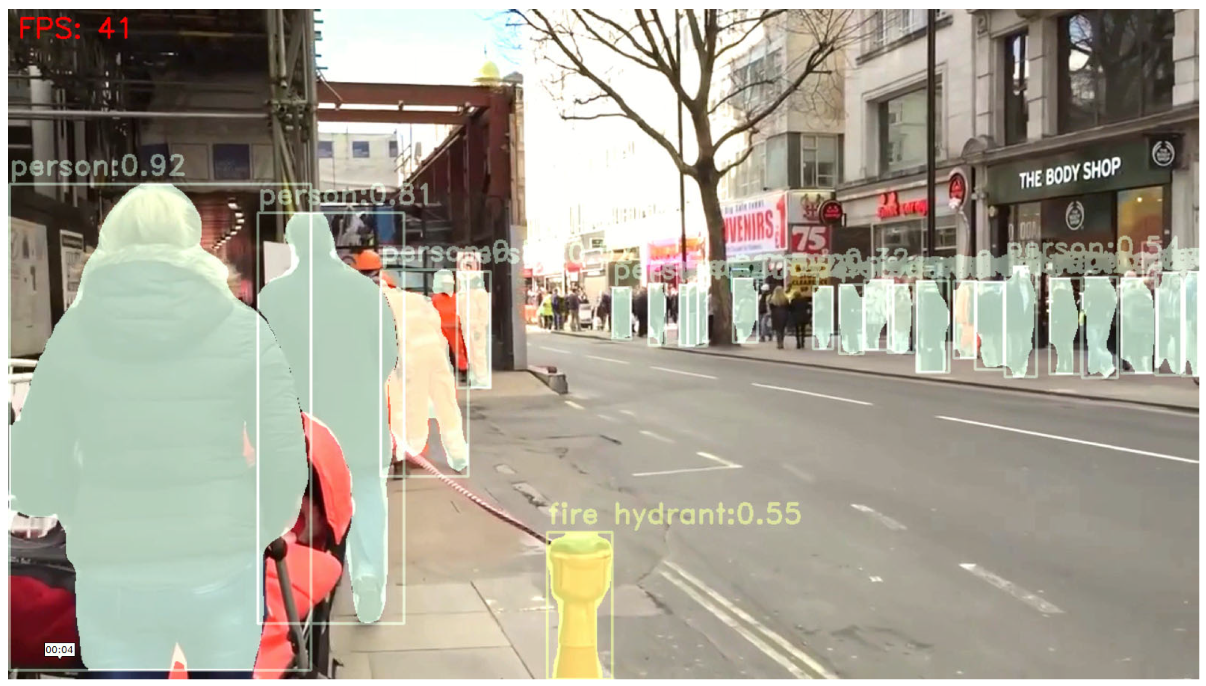
YOLO (You Only Look Once), a real-time object detection algorithm, was first proposed by Redmon et al. 2016 [23]. Unlike conventional object detection approaches, YOLO formulates the detection task as a unified regression problem that directly maps image pixels to bounding box coordinates and class probabilities, achieving exceptional detection speed while maintaining competitive accuracy. Our implementation operates through the Open Computer Vision Library (OpenCV) Deep Neural Networks (DNN) framework, requiring no dependencies on deep learning libraries and maintaining complete independence. With GPU acceleration, the system achieves 40 frames per second (FPS) detection throughput, fully satisfying real-time computational requirements. As shown in Figure 1.

By integrating a semantic segmentation module (YOLOv10), the system accesses segmentation results in real time via a dedicated processing thread. The framework first identifies potential dynamic objects in the image stream and then verifies their dynamic properties using epipolar line constraints and geometric consistency checks. This integrated approach effectively reduces error propagation caused by back-end feature point matching and reprojection processes. 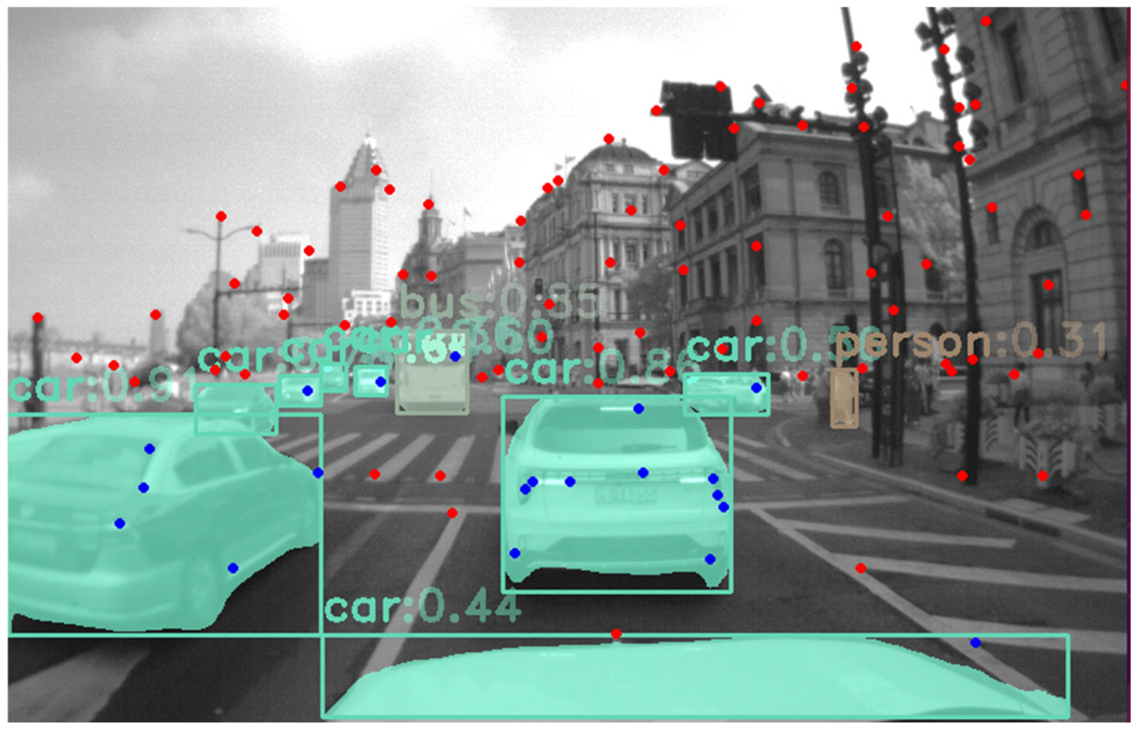Figure 2 gives the results of pixel-level semantic segmentation and dynamic target detection for the vision front-end, wherein the red points indicate static feature points and the blue points indicate dynamic feature points that need to be rejected after detection and identification.

As can be observed, the YOLO module in the visual image accurately identifies, filters, and removes feature points on dynamic objects such as vehicles and pedestrians in the scene. This ensures that dynamic feature points introduce minimal error during the construction of the visual reprojection error in the back-end. The dynamic point detection process in this paper consists of the following steps: First, normal feature point extraction is performed on the current frame of the image. Next, the semantic segmentation results of the current frame from the semantic segmentation thread are obtained, and all feature points to be inspected that fall within the semantic segmentation regions are marked. Then, RANdom Sample Consensus (RANSAC) is used to identify the fundamental matrix with the largest outliers. Subsequently, the fundamental matrix is utilized to compute the epipolar lines for the current frame. Finally, it is determined whether the distance between the matched points and their corresponding epipolar lines is less than a certain threshold. If the distance exceeds the threshold, the matched point is judged to be moving based on the epipolar line constraint, which effectively filters out dynamic feature points.

To reduce the computational load required for semantic segmentation, we first perform feature extraction and keyframe selection on the image. Semantic segmentation is executed only when a frame is identified as a keyframe, significantly reducing the number of images requiring semantic segmentation. Additionally, since semantic recognition is applied solely to keyframes, discontinuities between consecutive frames may arise. To prevent missed detections, we predict the previously recognized results based on pixel motion velocity and direction, incorporating the predicted outcomes into the dynamic detection interval. This approach enhances recognition accuracy through geometric consistency constraints.

The proposed system utilizes a pre-trained model on the Microsoft Common Objects in Context (COCO) dataset, selecting 19 classes from the original 80 categories as high-motion probability objects: a person, bicycle, car, motorcycle, airplane, bus, train, truck, boat, bird, cat, dog, horse, sheep, cow, elephant, bear, zebra, and giraffe. By leveraging pixel-wise semantic labels, this configuration provides prior knowledge about the motion characteristics of these objects. The selected classes comprehensively represent typical dynamic entities encountered in autonomous driving scenarios, fully addressing current operational requirements.

3.2. Epipolar Line Constraint Method

For the matched feature point pairs in the previous frame and current frame images, with their coordinates denoted as $p_i=[u_i,v_i,1]$ and $q_i=[u_i,v_i,1]$, respectively, the epipolar line constraint can be expressed as follows:

$$E(i)=q_i^T{l}_2=q_i^{T}F{p}_i=0$$

(8)

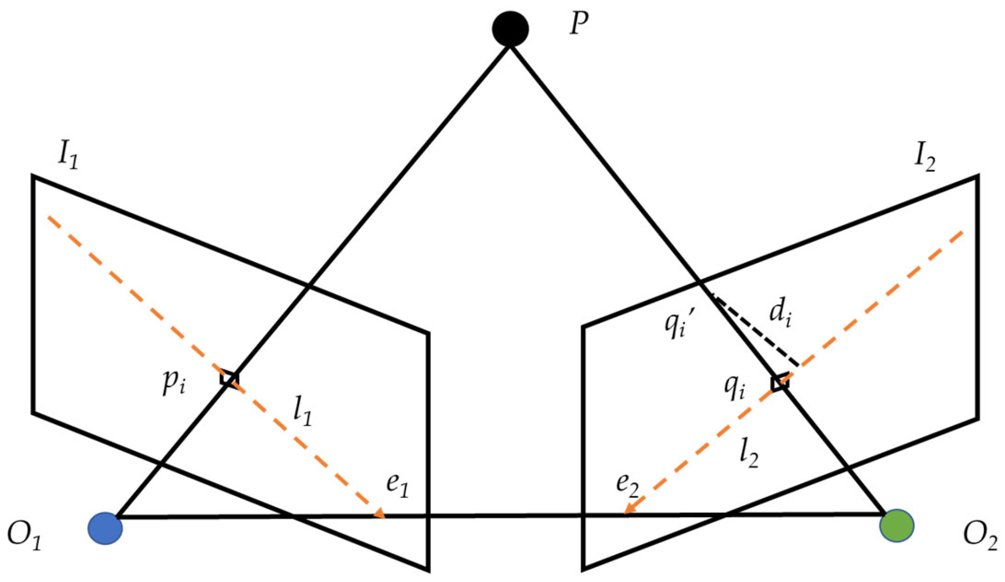
where $l_2$ is s the pole line corresponding to $q_i$ in the current frame. The projection of point $P$ on the second frame image must lie on the epipolar line $l_2$. However, interference from dynamic objects causes the aforementioned epipolar line constraint to fail. The distance between feature point $q_i$ and its corresponding epipolar line $l=Ax+By+C=0$ is defined as follows:

$$D={\displaystyle \frac{\left|A{u}_i^q+B{v}_i^q+C\right|}{\sqrt{A^2+B^2}}}={\displaystyle \frac{\left|q_i^{\mathrm{T}}F{q}_i\right|}{\sqrt{A^2+B^2}}}.$$

(9)

The epipolar line constraint distance of static feature points is relatively small, whereas that of dynamic feature points is typically significantly larger. When dynamic feature points move along the epipolar line, the epipolar line constraint distance between them may also become relatively small, potentially leading to the inaccurate identification of moving dynamic feature points. Therefore, in addition to employing the epipolar line constraint, it is necessary to incorporate supplementary methods to provide additional constraints, thereby ensuring the comprehensive identification of dynamic feature points within the scene. The schematic diagram of the epipolar line constraint is shown in Figure 3.

3.3. Geometric Consistency Constraints

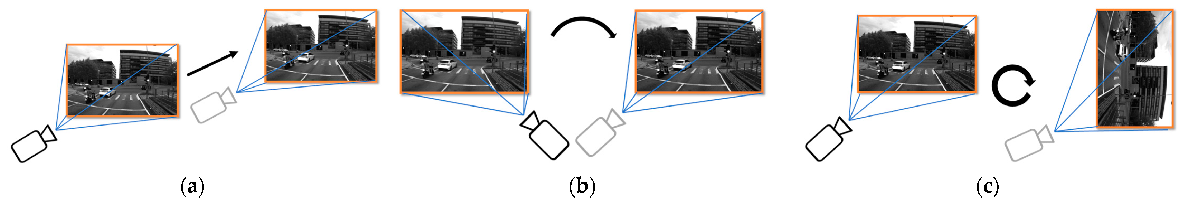
The geometric consistency verification is primarily determined through the motion vectors of feature points. Camera motion can generally be categorized into linear motion Figure 4a and rotation, with rotation further divided into turning Figure 4b and rolling Figure 4c. Since rolling (rotation around the image center) typically does not occur in vehicular scenarios, this discussion focuses exclusively on linear motion and panning.

For linear camera motion, the velocity or displacement vectors of extracted feature points across the entire image exhibit left–right symmetry with smaller magnitudes near the image center and larger magnitudes toward the periphery. In the panning motion, the feature point vectors demonstrate approximately uniform direction and magnitude characteristics throughout the image. The rolling motion would produce vectors with identical magnitudes but varying directions, though this scenario is excluded from consideration in vehicular applications due to the absence of image-center rotation.

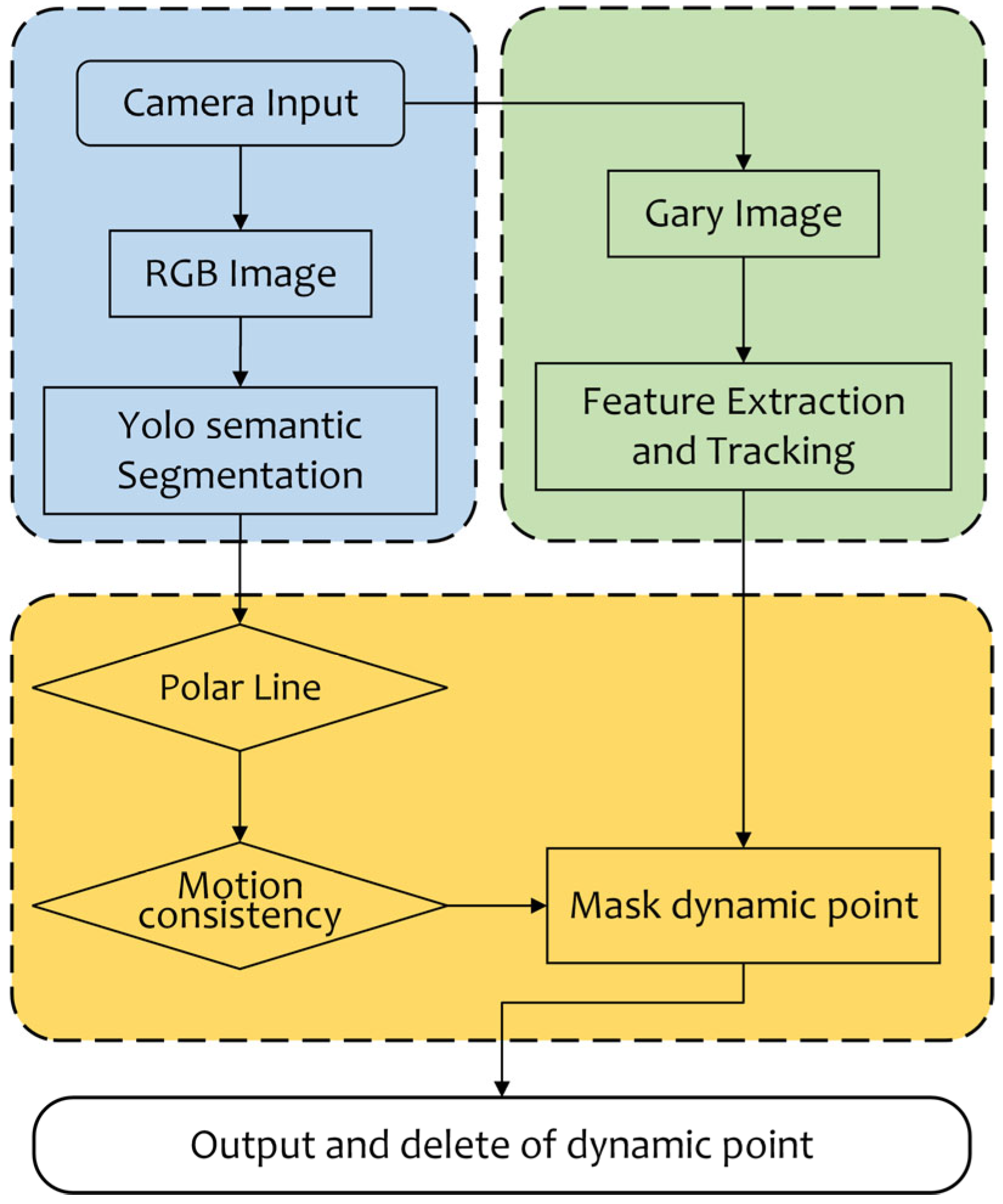
In vehicular scenarios, the primary camera motion modes are limited to linear motion and horizontal rotation. Consequently, geometric consistency verification becomes relatively straightforward for such environments. By leveraging segmentation results directly obtained from the semantic segmentation thread, dynamic feature points can be accurately identified through consistency checks between target regions segmented semantically and the global image context. The workflow for visual feature extraction and dynamic feature recognition is illustrated in Figure 5.

The acquired grayscale and RGB images from the data input interface undergo parallel processing through two independent threads: one dedicated to feature point extraction and tracking, while the other concurrently performs semantic segmentation on the corresponding RGB image data. Subsequently, the extracted features and semantic information are fused, enabling the comprehensive attribute recognition of feature points through integration with additional dynamic detection algorithms.

4. A New Stochastic Model for GNSS RTK

4.1. RTK Error Model

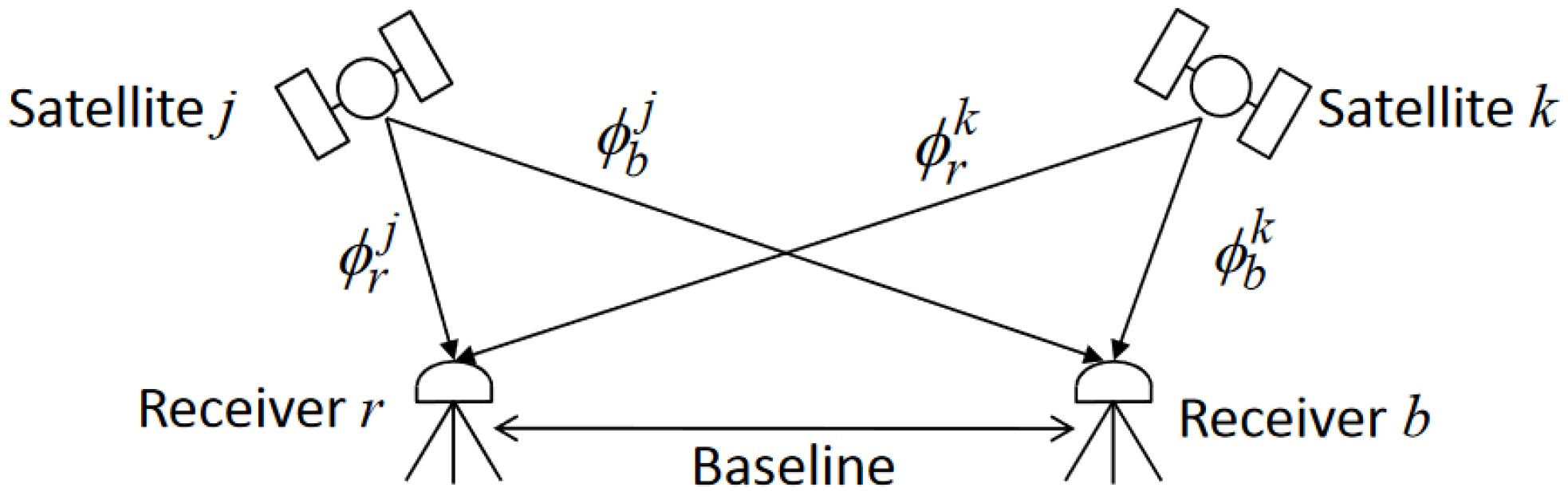
Differential observation models can simplify the localization model by eliminating or weakening the effects of observation errors that are mostly the same or have strong spatial correlation. The disadvantages are low data utilization and the introduction of correlation between observations, which makes processing more difficult. The principle of RTK differential observation is shown in Figure 6.

In urban canyon scenarios, radio signals are highly susceptible to specular reflections. Reference stations for RTK are typically deployed in areas with favorable observation conditions, avoiding regions severely affected by NLOS and multipath errors. In contrast, observation data from rover stations in complex urban environments often contain significant NLOS and multipath errors. The substantial disparity in observation environments between reference and rover stations renders differentiation techniques ineffective in fully eliminating residual errors caused by these environmental discrepancies.

Considering the correlation error and measurement noise, the GNSS observation equation in meters can be expressed as follows:

$$\left\{\begin{array}{l}\begin{array}{l}{P}_{r,k}^s={\rho }_r^s+c\left(t_r-t^s\right)+{\gamma }_k\cdot I_{r,k}^s+m_r^s\cdot zw{d}_r+b_{r,k}-b_k^s+{\epsilon }_{P_k}\\ L_{r,k}^s={\rho }_r^s+c\left(t_r-t^s\right)-{\gamma }_k\cdot I_{r,k}^s+m_r^s\cdot zw{d}_r+{\lambda }_k\cdot N_{r,k}^s+{\lambda }_k\left(B_{r,k}-B_k^s\right)+{\epsilon }_{L_k}\end{array}\hfill \end{array}\right.,$$

(10)

where $P$ and $L$ denote pseudo-range and phase observations, respectively. $\rho$ denotes the geometric distance between the satellite $s$ and the receiver $r$. $t_r$ and $t^s$ denote the receiver and satellite clock bias, respectively. $c$ is denotes the speed of light. $I_{r,1}^s$ denotes the slant path ionospheric delay of satellite s at frequency 1. $k$ is the signal frequency. ${\gamma }_k=f_1^2/f_k^2$ is a frequency-dependent ionospheric delay factor. $zw{d}_r$ and $m$ denote the zenith tropospheric delay and the corresponding mapping function, respectively. $N$ is ambiguity of whole cycles. $\lambda$ is wavelength. $b_r$ and $b^s$ denote the receiver-side and satellite-side pseudo-range hardware delays, respectively. $B_r$ and $B^s$ denote the receiver-side and satellite-side phase hardware delays, respectively. ${\epsilon }_L$ and ${\epsilon }_P$ denote the observation noise and multipath error for phase and pseudo-range measurements, respectively.

Assuming the distance between the reference station and the rover is relatively short, the atmospheric delay errors can be considered identical and relatively stable. By differentiating the observations between the reference station and the rover, the impact of atmospheric delay errors can be directly eliminated. Let the reference satellite be $i$; the variances of the between-station single-difference observations for pseudo-range and phase are as follows:

$$\left\{\begin{array}{l}\mathrm{\Delta }{P}_{b,r,k}^s=\mathrm{\Delta }{\rho }_{b,r,k}^s+c(t_r-t^s)+\mathrm{\Delta }{I}_{b,r,k}^s+\mathrm{\Delta }{T}_{b,r,k}^s+\mathrm{\Delta }{b}_{b,r,k}+\mathrm{\Delta }{\epsilon }_{b,r,k}^s\\ \mathrm{\Delta }{L}_{b,r,k}^s=\mathrm{\Delta }{\rho }_{b,r,k}^s+c(t_r-t^s)+\mathrm{\Delta }{I}_{b,r,k}^s+\mathrm{\Delta }{T}_{b,r,k}^s+{\lambda }_k\mathrm{\Delta }{N}_{b,r,k}+\mathrm{\Delta }{B}_{b,r,k}+\mathrm{\Delta }{\epsilon }_{b,r,k}^s\end{array}\right.$$

(11)

where $\mathrm{\Delta }{T}_{b,r}^s$ is the differential atmospheric delay errors, which can be considered to be zero in short-baseline RTK. $\mathrm{\Delta }{b}_{b,r,k}=b_{r,k}^s-b_{b,k}^s$, $\mathrm{\Delta }{B}_{b,r,k}=B_{r,k}^s-B_{b,k}^s$. Differentiating the above single-difference observation equations between satellites gives the double-difference observation model as follows:

$$\left\{\begin{array}{l}\mathrm{\Delta }\nabla P_{r,b,k}^{i,j}=\mathrm{\Delta }\nabla {\rho }_{r,b,k}^{i,j}+\mathrm{\Delta }\nabla {\epsilon }_{P_{r,b,k}}\\ \mathrm{\Delta }\nabla L_{r,b,k}^{i,j}=\mathrm{\Delta }\nabla {\rho }_{r,b,k}^{i,j}+{\lambda }_k\mathrm{\Delta }\nabla N_{r,b,k}^{i,j}+\mathrm{\Delta }\nabla {\epsilon }_{L_{r,b,k}}\end{array}\right.$$

(12)

$\mathrm{\Delta }\nabla N_{r,b,k}^{i,j}=\mathrm{\Delta }{N}_{r,b,k}^i-\mathrm{\Delta }{N}_{r,b,k}^j$. $\mathrm{\Delta }\nabla {\epsilon }_{P_{r,b,k}}$ and $\mathrm{\Delta }\nabla {\epsilon }_{L_{r,b,k}}$ represent the differences between the observation noise of satellite $i$ at the rover and the reference station, and the differences between the observation noise of satellite $j$ at the rover and the reference station, respectively. For the same satellite, the noise level at the satellite end is identical, and most of the satellite end errors can be eliminated through between-station differentiating. However, for the same receiver, the noise levels for different satellites may vary and could even differ significantly. Therefore, differentiating across different satellites cannot completely eliminate the impact of observation noise at the receiver end.

Through the detailed derivation and error analysis of the RTK observation equations, we find that most errors have been eliminated after applying between-station and between-satellite differentiating. The remaining error terms in the double-difference observations consist of the residual double-difference observation noise, which includes noise, residual multipath, and NLOS errors.

4.2. An Adaptive Weighting Strategy for GNSS RTK

Generally, GNSS signal quality exhibits strong correlation with satellite elevation angles [33], which is related to the physical characteristics of electromagnetic waves. When propagating through different media, larger incidence angles induce greater path bending of the signal, which manifests as increased ranging errors in the observed data. The elevation angle-dependent stochastic model can be expressed as follows:

$${\sigma }^2(el)=\left\{\begin{array}{ll}{\sigma }_0^2\hfill & el⩾{30}^{°}\hfill \\ {\displaystyle \frac{{\sigma }_0^2}{{\sin }^2(el)}}\hfill & el<{30}^{°}\hfill \end{array}\right.,$$

(13)

where ${\sigma }_0^2$ is the a priori variance of the observations and $el$ is the angle of altitude.

The elevation angle-based modeling approach primarily addresses conventional physical models and does not account for NLOS and multipath errors caused by electromagnetic wave refraction and superposition phenomena in special environments. In the unique environment of urban canyons, the stochastic model based on elevation angle can no longer accurately reflect the quality of observation information. Therefore, there is a need for a new GNSS stochastic model specifically adapted to urban canyon environments.

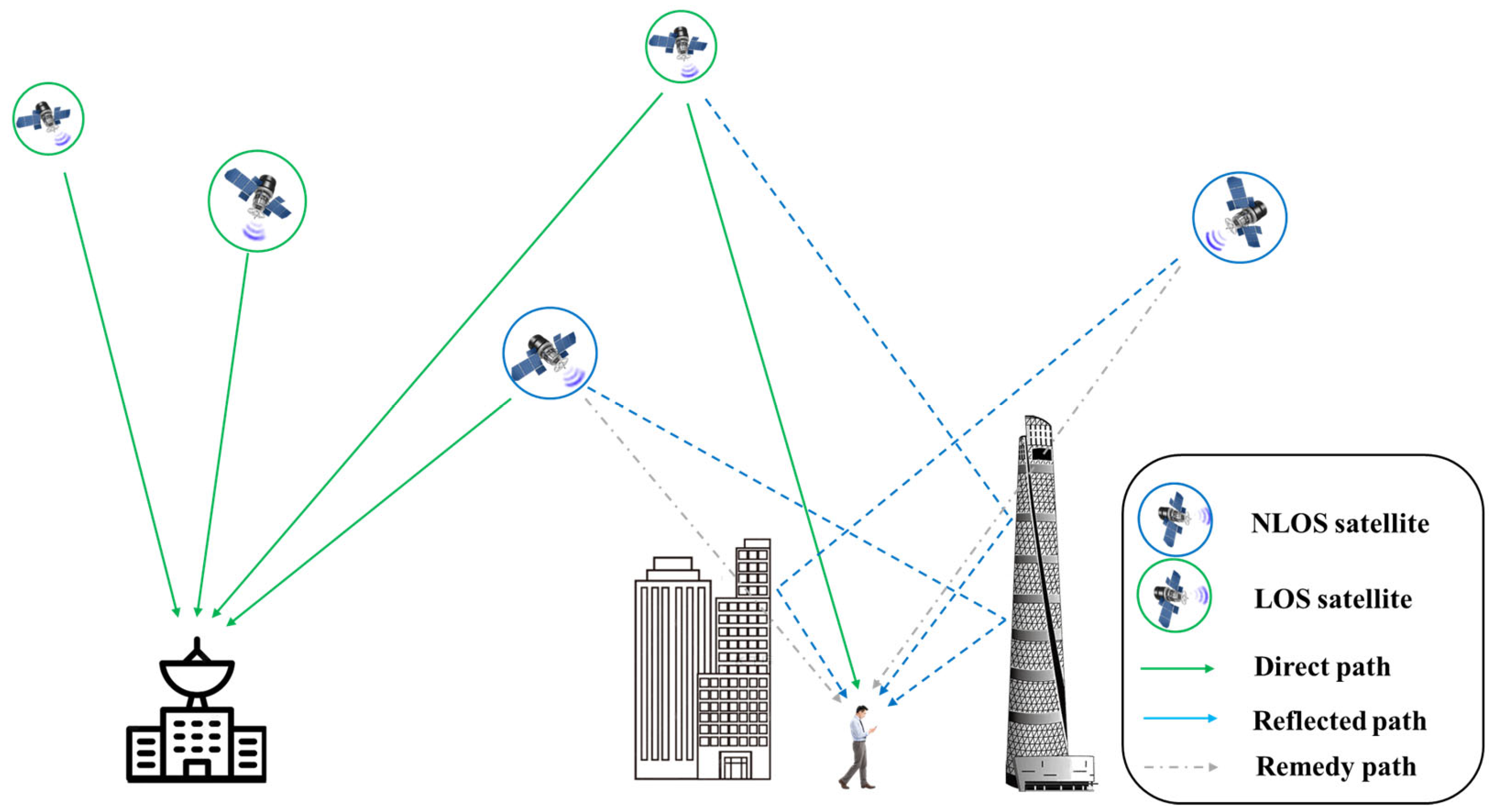
Multipath errors refer to inaccuracies that occur when a receiver captures not only the direct signal from a transmitter but also one or more signals arriving via reflected paths. These reflections may originate from surfaces such as ground terrain, buildings, or vehicles. Since these additional paths are longer than the direct path, the reflected signals arrive at the receiver with delays and interfere with the direct signal, thereby introducing measurement errors. NLOS errors specifically describe scenarios where the direct signal from the transmitter cannot be received under line-of-sight (LOS) conditions. When obstacles block the direct path between the transmitter and receiver, creating NLOS conditions (as illustrated in Figure 7), the receiver can only capture reflected, diffracted, or scattered signals. This leads to ranging errors, particularly degrading positioning accuracy in TOA (Time of Arrival) or TDOA (Time Difference of Arrival)-based systems. Due to the abundance of reflective surfaces, both error types are highly prevalent in the specialized environment of urban canyons.

Through the analysis of the double-differenced observation model in RTK, we recognize that after double-differentiating the observations, only the observation noise (including NLOS and multipath errors) remains in the measurement equation. For the special scenario of urban canyons, where significant environmental differences exist between the rover and reference station observation conditions, we posit that substantial errors persist in the differential noise term.

Secondly, as pseudo-range measurements contain considerable errors whose magnitudes cannot be precisely determined [34], incorporating pseudo-range observations may degrade positioning accuracy. Therefore, high-precision positioning algorithms typically apply down-weighting to pseudo-range observations. This does not imply that pseudo-range data are entirely unusable, but rather stems from the general inability to quantify their error components. In urban canyon environments where signal obstruction drastically reduces observable satellites, every measurement becomes critically valuable. Thus, effectively utilizing all available observational data becomes paramount in such settings.

Analyzing fundamental GNSS principles and observation equations reveals that carrier phase measurements exhibit significantly higher precision than pseudo-range code measurements. Based on this property, we introduce Code-Minus-Phase (CMP) observations to quantify the quality of pseudo-range observations [35,36]. CMP observations are conventionally employed to characterize multipath errors in pseudo-range measurements.

To enhance GNSS observation quantity and usability in complex urban environments, our proposed method utilizes CMP to quantify pseudo-range noise levels, enabling adaptive weight adjustment for participating observations based on error magnitudes. This approach substantially improves data utilization efficiency while enhancing system accuracy and availability.

The code pseudo-range ($P$) and carrier phase ($L$) observations are given in meters by the following equations:

$$\left\{\begin{array}{l}{P}_r^s={\rho }_r^s+c\left(d{t}_r-d{t}^s\right)+T_r^s+I_r^s+c\left(b_r-b^s\right)+\epsilon \left(P_r^s\right)\\ L_r^s={\rho }_r^s+c\left(d{t}_r-d{t}^s\right)+T_r^s-I_r^s+c\left(B_r-B^s\right)+\lambda N_r^s+\epsilon \left(L_r^s\right)\end{array}\right..$$

(14)

$CMP$ observations can be written in the following form:

$$CM{P}_r^s=P_r^s-L_r^s=2I_r^s+c\left(b_r-b^s\right)-c\left(B_r-B^s\right)-\lambda N_r^s+\epsilon (P_r^s-L_r^s)$$

(15)

The subtraction of phase observations from pseudo-range observations eliminates the geometry-related terms, including receiver and satellite clock offsets, tropospheric delays, and geometric range. The resulting $CMP$ combination still contains twice the ionospheric delay, hardware delay biases, multipath effects, and observation noise. Since the observation noise and multipath effects in phase observations are significantly lower than those in pseudo-range observations, their impacts can be neglected in the $CMP$ combination.

Applying epoch differentiating to $CMP$ observations yields the following result:

$$\mathrm{\Delta }CMP={\displaystyle \frac{1}{\mathrm{\Delta }t}}(CM{P}_k-CM{P}_{k-1})=2I_r^s+M{P}_k+{\epsilon }_k$$

(16)

It can be observed that differentiating the $CMP$ observations between epochs leaves only the multipath and twice the ionospheric delay. The ionospheric delay can be eliminated through modeling. Through this quantitative method for estimating pseudo-range multipath errors, we proposed a stochastic model suitable for urban canyons to enhance the weighting of pseudo-range observations. The stochastic model is constructed as follows:

$${\sigma }^2(\mathrm{\Delta }CMP)={\displaystyle \frac{{\sigma }_0^2}{{\sin }^2(\mathrm{\Delta }CMP)}}$$

(17)

where $\mathrm{\Delta }CMP$ is the difference of $CMP$.

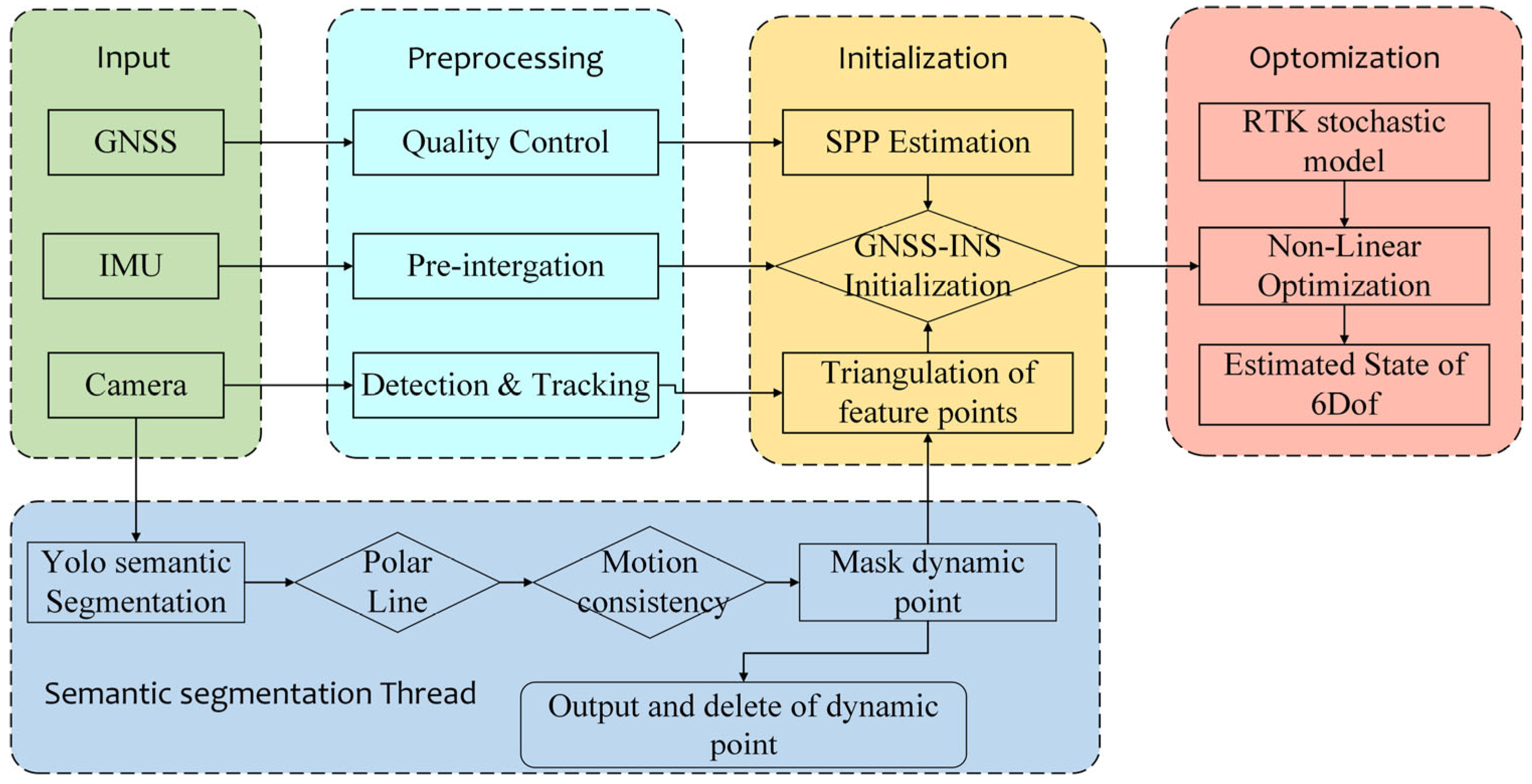
Figure 8 gives the basic flow of the system operation. This system adopts a multi-source heterogeneous sensor fusion architecture, integrating observation data from the GNSS, IMU, and vision sensors. Robust positioning in complex scenarios is achieved through hierarchical processing and optimization algorithms. During the data preprocessing stage, dynamic weighted quality control based on quality factor evaluation is implemented for GNSS observations, while pre-integration operations are performed on raw IMU data to construct kinematic constraint models. For vision data streams, a dual parallel processing architecture based on feature tracking and semantic parsing is innovatively designed: the feature extraction thread achieves inter-frame feature matching via the optical flow method, while the semantic segmentation thread employs deep convolutional networks for scene understanding, providing prior constraints for subsequent nonlinear optimization.

The positioning solution phase employs a hierarchical progressive fusion strategy: first, an a priori coordinate reference is obtained through GNSS SPP, followed by an improved RTK stochastic model to achieve adaptive observation weighting. This is combined with INS mechanization equations to establish a tightly coupled navigation framework. For the vision subsystem, a multi-constraint dynamic object suppression algorithm is proposed, effectively eliminating interference from dynamic feature points by fusing semantic segmentation results with epipolar line constraints and motion consistency verification. Finally, the spatiotemporal unification and global optimal estimation of multi-source observations are realized through sliding window optimization.

5. Experiments and Analysis

5.1. Visual Dynamic Object Detection Experiment

We tested and compared the algorithm performance using the open-source urban environment in-vehicle multi-source fusion dataset from Shanghai. For the GNSS, we utilized dual-frequency raw carrier phase, pseudo-range, and Doppler observations from four constellations: GPS (L1/L5), GLONASS (G1/G2), Galileo (E1/E5a), and BDS (B1/B3), sampled at 10 Hz. Camera data were captured at a resolution of 752 × 480 pixels with a 10 Hz frequency. The IMU operated at a sampling rate of 200 Hz. The key equipment performance parameters can be found in [8]. The ground reference truth is derived from the post-processed integrated navigation results obtained by using the IE 8.90 (Inertial Explorer) software to process data from GNSS and high-precision fiber optic IMU. To validate the effectiveness of the algorithm, we selected a representative dataset (5.2) under typical complex urban environmental conditions as an example. The 3D residual sequences of positioning following the detection and removal of dynamic objects in visual images are compared with those of the original algorithm, as shown in Figure 9.

As observed in Figure 9, visual dynamic targets can severely impact the performance of the RTK/INS/Vision multi-source fusion navigation algorithm. When a large number of dynamic targets in visual perception cannot be accurately detected and eliminated, significant positioning errors may occur in three-dimensional directions during periods such as 25,800–26,200 s. In contrast, the integration of a dynamic target detection algorithm enables the effective identification of visual dynamic targets. By comprehensively applying multiple methods for precise elimination, the accuracy of the multi-source fusion algorithm can be substantially enhanced.

Since we established a separate thread utilizing GPU acceleration to perform YOLO-based image semantic segmentation, our image processing module consumes minimal additional time and achieves real-time processing capability. The GPU employed in this implementation is an NVIDIA GeForce RTX 2060 (Laptop) (NVIDIA, Santa Clara, CA, USA).

5.2. GNSS RTK Stochastic Mode Experiments

To validate the performance of the proposed new stochastic model, dedicated tests were conducted on the GNSS RTK stochastic model. Taking the urban complex vehicular environment dataset (Dataset 5.2) as an example, a comparative analysis of the residual sequences between the proposed model and the original algorithm is presented in Figure 10.

As shown in Figure 10, degraded observation data quality and a reduced number of visible satellites during specific time intervals—caused by issues such as obstructions—result in increased positioning errors in the multi-source fusion system. Without altering other parameters or conditions, the implementation of a new stochastic model in GNSS RTK significantly enhances system accuracy, demonstrating notable performance improvement.

5.3. Multi-Source Fusion Experiment

To further evaluate the algorithm’s performance, multiple tests were conducted using a classic complex urban vehicular dataset (4.1). This dataset encompasses typical urban road scenarios, including urban canyons, urban roads, and interactions with vehicles and pedestrians. The experiments were divided into four schemes, with the specific configurations as follows:

Scheme A: The original RTK/INS/Vision algorithm results without adding any enhancement strategies (symbols: w/o CMP and detect). Scheme B: The original RTK/INS/Vision algorithm augmented with vision-based feature detection and removal (symbols: w/detect). Scheme C: The original RTK/INS/Vision algorithm augmented with a stochastic weighted RTK model for urban canyons (symbols: w/CMP). Scheme D: The original RTK/INS/Vision algorithm incorporating both vision-based dynamic feature detection/removal and the stochastic urban canyon RTK model (symbols: w/CMP and detect).

Figure 11 presents the visible satellite count and Geometric Dilution of Precision (GDOP) sequences for this dataset. The results reveal intermittent drastic fluctuations in satellite visibility under urban canyon conditions, with the minimum number of visible satellites dropping below 5 and the maximum GDOP exceeding 25. These factors impose significant challenges on conventional RTK positioning.

The positioning residual sequences of multiple tested schemes are illustrated in Figure 12. The green line indicates the sequence of positional residuals for Scheme A. The blue line indicates the sequence of positional residuals for Scheme B. The red line indicates the sequence of positional residuals for Scheme C, while the black line indicates the sequence of positional residuals for Scheme D.

It can be observed that Scheme B (with dynamic object removal in visual imagery) significantly improves multi-source fusion positioning accuracy in urban environments. Scheme C (with urban canyon RTK stochastic model) also effectively enhances RTK/INS/Vision multi-source fusion positioning accuracy. Scheme D, which integrates both dynamic object detection strategies and the GNSS urban canyon stochastic model, achieves optimal overall positioning accuracy. The precision statistics of all four schemes are summarized in

Table 1. Accuracy statistics of positioning algorithms.

	E (m)	N (m)	U (m)	3D (m)	Promote
Scheme A	0.188	0.186	0.123	0.291	-
Scheme B	0.161	0.188	0.1176	0.274	5.84%
Scheme C	0.166	0.185	0.066	0.257	11.68%
Scheme D	0.164	0.183	0.064	0.253	13.05%

.

6. Discussion

In order to show the differences of several algorithms more intuitively, we have counted the 3D positioning error distributions of the four schemes, as shown in Figure 13.

As observed, Schemes C and D demonstrate the most concentrated error distributions, with 95% of errors below 0.5 m. Scheme B achieves 90% of errors within 0.5 m, while the conventional multi-source fusion algorithm (Scheme A) only attains approximately 60% of errors below 0.5 m. Scheme D exhibits the most concentrated overall error distribution, demonstrating that the proposed vision-based dynamic object detection algorithm and stochastic urban canyon model in the multi-source fusion framework effectively enhance positioning accuracy.

It is noteworthy that our strategy effectively improves the RTK ambiguity fixation rate in multi-source fusion algorithms. For Dataset 4.1, the ambiguity fixation rates are 46.3% for Scheme A, 60.1% for Scheme B, 67.1% for Scheme C, and 67% for Scheme D. The results demonstrate that removing dynamic elements from visual observations significantly enhances the RTK ambiguity fixation rate in RTK/INS/Vision multi-source fusion. The enhanced algorithm incorporating two strategies achieves improvement percentages in ambiguity fixation rates of 44.7%, 123.8%, and 42.1% compared to the original algorithm across three typical urban complex environment datasets (4.1, 5.1, 5.2).

Table 2. RTK ambiguity fixing rate of multi-source fusion algorithm.

	Scheme A	Scheme B	Scheme C	Scheme D	Improvement
4.1	46.3%	60.1%	67.1%	67%	44.7%
5.1	24.7%	46%	55.9%	55.3%	123.8%
5.2	49.4%	61%	68.4%	70.2%	42.1%

presents the ambiguity fixation rates under different schemes for the three datasets.

It can be observed from the data in the table that the new stochastic RTK model achieves greater positioning performance improvements than the vision-based dynamic object detection and removal algorithm across all three datasets. Figure 14a presents the trajectory in a typical urban complex environment (Dataset 4.1) along with schematic diagrams of urban canyon occlusions.

Figure 14b gives the trajectories of the carriers obtained by solving the Dataset 5.1 set for each of the four multi-source fusion navigation schemes. It can be seen that the trajectories of the schemes with the augmentation strategies attached are able to suppress the systematic errors better in some special regions compared to the multi-source fusion schemes, without adding any strategies.

7. Conclusions

In this study, we propose a multi-source fusion algorithm designed for urban canyons to enhance the accuracy and availability of systems in complex urban environments. First, we introduce a neural network-based dynamic object detection and removal algorithm into the visual framework. This algorithm accurately identifies regions containing dynamic objects and combines epipolar line constraints with geometric consistency constraints to confirm the dynamic attributes of these objects. Second, to address the issues of low GNSS observation quality and limited visible satellites in urban canyon environments, we propose an adaptive weighting GNSS RTK stochastic model based on the quantitative assessment of pseudo-range error magnitudes. The evaluation results on public datasets demonstrate that the proposed RTK/INS/Visual multi-source fusion algorithm improves positioning accuracy by 44.7%, 123.8%, and 42.1%, respectively, compared to traditional methods. This effectively enhances the accuracy and availability of positioning algorithms in complex urban environments. In future work, we will explore more robust adaptive fusion algorithms for multi-sensor observations.