Abstract
Mesoscale eddies induce significant variations in the temperature and salinity of the upper ocean, thereby exerting a substantial impact on sound propagation. Specifically, they can form or dissipate surface sound channels (SCs) and subsurface sound channels (SSCs). However, the specific impact of mesoscale eddies remains unclear at present. In this paper, META2.0, Argo, and SODA are employed to analyze the sound propagation characteristics of mesoscale eddies in the Kuroshio Extension (KE) by using a composite analysis method and a ray-tracing model. Results demonstrate that cyclonic eddies (CEs) cause the disappearance of the original SCs in winter, while simultaneously generating SSCs. Conversely, anticyclonic eddies (AEs) induce SCs in spring and winter, while in summer they induce SSCs and in autumn create dual-duct sound channels (DCs). This study quantitatively reveals the influence of mesoscale eddies on the genesis and demise of SCs and SSCs, providing technical support for sonar equipment to utilize mesoscale eddies.
1. Introduction
Mesoscale eddies are ubiquitous in the ocean [1,2,3,4]. It has been a focal point of extensive global research over the past four decades, leveraging a combination of in situ measurements, satellite surveillance, and computational modeling techniques [5]. However, in situ data primarily serve to analyze the structure of individual mesoscale eddies, while satellite observations are limited to capturing sea surface characteristics. Additionally, model outcomes may encompass certain uncertainties and inaccuracies [6]. The research on eddy underwater structures has consistently been hampered by the dearth of underwater observational data [7]. Under these conditions, Argo has been scaled up to constitute a principal element within the global oceanographic observation infrastructure. Its observational data are predominantly employed for the analysis of the multifaceted structure of mesoscale oceanic eddies. For example, by utilizing altimetry and Argo data, the mean 3D eddy structure in the eastern South Pacific was reconstructed [8]. Moreover, a regionally correlated parameter model for eddy-induced sound speed anomaly structures has been formulated [9].
The influence of mesoscale eddies on the underwater sound speed field can extend to a depth of 1000 m below the sea surface [10], thereby altering the distribution of acoustic properties in the upper-ocean layer [11]. By calculating the acoustic rays, it was observed that the propagation from a near-sea surface sound source within an eddy changes as it moves towards the sound fixing and ranging channel (SOFAR) axis [12]. Similarly, a moving eddy can also cause significant alterations in the propagation of acoustic rays [13]. Utilizing a parameterized eddy model, precise expressions for the phase variation of each acoustic ray were yielded [14]. Moreover, it was found that as sound waves propagate from outside to inside the eddy, the convergence zone distance gradually decreases [15]. Through official experiments, it was discovered that warm eddies can extend the horizontal span of the convergence zone and make it wider [16]. Furthermore, warm currents from the Pacific can alter the conventional single surface sound channel in the Arctic and form a new subsurface sound channel between depths of 80 to 250 m [17].
Under certain conditions, mesoscale eddies can form surface ducts and subsurface ducts [18,19], enabling the long-distance propagation of sound waves [20,21]. Moreover, the impact of the eddies diminishes with increasing distance from the eddy center, resulting in various acoustic effects [22]. However, due to the scarcity of underwater observational data, the effects and mechanisms of mesoscale eddies on the surface and subsurface channels in the ocean are somewhat unclear, and related research is relatively scarce.
This study comprehensively utilizes underwater observational data and climatological reanalysis data, taking the Kuroshio Extension (140°E to 180°E, 30°N to 40°N) as the research area, to obtain the standardized underwater structure of eddies in this region. It calculates the impact of eddies of different polarities and intensities on the sound speed in the upper layer of seawater under different seasonal background fields, explains the mechanisms and patterns by which mesoscale eddies affect the surface and subsurface sound channels, and reveals the propagation characteristics of sound waves in the surface or subsurface sound channels affected by eddies.
2. Data and Methods
2.1. Datasets Ultilized in the Research
The study utilizes a total of three datasets: META 2.0, Argo, and SODA 3.4.2. The first two are used for eddy composite analysis, while SODA serves as the climatological reference to quantify mesoscale eddy-induced sound speed anomalies.
The Mesoscale Eddy Trajectories Atlas, version 2.0 (META 2.0), is primarily designed for specialized research on mesoscale eddies in the ocean. The raw data of the product originate from daily altimeter sampling by two satellites spanning from 1 January 1993 to 7 March 2020. These data underwent reanalysis and processing in accordance with the vortex identification and tracking methodology provided by Chelton [1]. It encompasses the sea surface characteristics of global ocean mesoscale eddies from 1 January 1993 to 7 March 2020. The main features include the amplitude of the eddy, eddy type, eddy center coordinates, observation sequence number, maximum average line speed, radius, observation date, trajectory identification number, etc. This dataset can provide a wealth of sea surface data for the composite of eddy subsurface structures.
Argo (Array for Real-time Geostrophic Oceanography) consists of oceanographic measurements including temperature, salinity, and other hydrological parameters. The dataset used in this paper is the Argo float profile dataset released by the Coriolis Center, which has undergone automatic quality control and processing. It selects underwater observational information recorded from 3 May 1998 to 11 January 2021, mainly including seawater pressure, temperature, salinity rate, buoy number, coordinates, etc. Argo can provide a rich set of underwater data for eddy compositing, thereby revealing the vertical structure of eddies.
SODA (Simple Ocean Data Assimilation) is a type of global ocean reanalysis data, including information on various marine parameters such as seawater temperature, seawater salinity, and seawater speed. This paper selects the SODA3.4.2 data from January 2000 to December 2019, which can provide the main results of the three-dimensional monthly average marine state variables mapped onto a regular 0.5° Mercator horizontal grid with 50 vertical depth layers. This can provide climatological data support for this study.
2.2. Data Processing Method
After quality control of the Argo data, the three-dimensional subsurface structure of mesoscale eddies in the study area is derived through composite analysis, thereby enabling the calculation of sound speed structures for typical mesoscale eddies across different seasons. Subsequently, the derived eddy parameters are input into the BELLHOP toolbox (version. 2020_11_4) to obtain the underwater sound speed profile structures of mesoscale eddies. This process reveals the acoustic fields associated with typical cyclonic and anticyclonic eddies, allowing further investigation of their impacts on (sub)surface sound channels and the characteristics of acoustic wave propagation within these channels.
Although the Argo data used have undergone automatic quality control, visual inspection of the plotted temperature and salinity profiles reveals issues such as missing variables, insufficient sampling points, and significant deviations from climatological means. To ensure the validity of subsequent analyses, further quality control on the Argo profiles is necessary. The specific quality control procedures are as follows:
- (1)
- Remove profiles with missing salinity or temperature data.
Some Argo observations prior to 2000 lack salinity or temperature records, making it impossible to calculate corresponding sound speed profiles. These profiles cannot be included in subsequent experiments. Therefore, all Argo files must be scanned to identify and delete those missing salinity or temperature profiles, retaining only files with complete temperature and salinity records. Profiles containing NaN (Not a Number) values in temperature or salinity data should also be discarded.
- (2)
- Exclude profiles with fewer than 10 depth sampling points or depths shallower than 1000 m.
Insufficient sampling points may lead to unrealistic temperature/salinity variations during vertical interpolation, compromising data reliability. Additionally, mesoscale eddies typically influence depths up to 1000 m, so Argo profiles must sample to at least this depth. Profiles failing to meet these criteria are filtered out.
- (3)
- Remove outliers using a 3-standard-deviation threshold.
After pairing Argo profiles with eddies and interpolating data to standardized depths (10:1:1000 m), compute the mean and standard deviation of temperature and salinity at each depth across all profiles. Profiles exceeding 3 standard deviations from the mean at any depth are identified as outliers and removed.
Subsurface temperature and salinity datasets from SODA and Argo programs enable the derivation of sound speed profiles through the application of Mackenzie’s empirical formula (Equation (1)).
In the formula, c denotes the sound speed (m/s), T represents temperature (°C), S indicates salinity (psu), and D corresponds to depth (m).
The composite analysis method can make use of a large number of asynchronously observed hydrological profile data and project them into the coordinate system with the eddy center as the origin, so as to form a scroll structure image under the statistical average, which can solve the data limitation problem well [7,8,23,24,25]. Given that Argo data capture mesoscale eddies of varying sizes, amplitudes, and polarities across different oceanic regions and time periods, a critical assumption must be established prior to applying composite analysis: within a geographically constrained study area, mesoscale eddies differ only in horizontal scale, amplitude, and polarity, while their fundamental structural characteristics remain consistent. In other words, the Argo-observed eddies included in the synthesis share an identical underlying structural framework.
In this method, the key is to identify all Argo profiles within the selected region and pair each profile with the eddy center that is closest in both time and space. The criteria set for eddy-Argo pairing in this study are as follows: (1) observations occur on the same day, and (2) the Argo profile falls within twice the radius of the eddy. The ratio of the distance between the buoy and the eddy center to the radius of the eddy is taken as the normalized distance of the buoy under the eddy coordinate system, i.e., . Then, the buoy is projected into the eddy coordinate system (Figure 1). The thermohaline profile data recorded by the composite eddy are used as the distribution of thermohaline in the water. After all the Argo projections are completed, the temperature and salinity data of the climate state are subtracted, and after data smoothing and sound speed calculation, the abnormal structure of the underwater sound speed of the eddy can be obtained. Finally, structures of eddies with different amplitudes can be obtained by normalization and restoration of amplitudes and polarities. The surface characteristics of the eddies, including their center positions and radii, were derived from the AVISO product, while the discrete in situ temperature and salinity profiles at subsurface depths were acquired from the Argo floats, and the climatological data were from SODA 3.4.2.
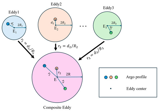
Figure 1.
Schematic diagram of eddy composite analysis.
The Acoustic Toolbox is a suite of ocean sound propagation modeling tools under the library of ocean acoustics. The BELLHOP toolbox within it is designed for ocean acoustic modeling and simulation. It is an acoustic propagation simulation program based on the ray-tracing method, specifically for simulating the propagation and scattering of sound waves in the marine environment. After the relevant environmental files are input, it can calculate the corresponding underwater sound pressure field and extract acoustic features. When inputting the mesoscale eddy-induced sound speed field into the BELLHOP acoustic toolbox for sound propagation loss calculation, it is first necessary to determine whether a surface or subsurface sound channel exists within the field. If a surface channel is present, the sound source is placed at the sea surface; if only a subsurface channel exists, the source is positioned at the depth of the subsurface channel axis. Simulations are then executed using Run Type R (ray-tracing) and Run Type C (coherent transmission loss) to derive the acoustic ray distribution and propagation loss characteristics under the influence of the mesoscale eddy. The key steps include generating corresponding “.env” and “.ssp” files from the sound speed field, configuring the source frequency to 3000 Hz, setting the top boundary condition to “QVW,” and determining the source location based on the identified channel type. This workflow ultimately produces the underwater acoustic field structure and energy attenuation patterns caused by the mesoscale eddy.
3. Results
3.1. Characteristics of Mesoscale Eddies in the KE
Satellite altimetry serves as an effective observational tool for mesoscale eddies, with the acquired data providing a robust basis for the investigation of surface characteristics of these eddies. Mesoscale eddy trajectory atlas indicates that between 1 March 1993 and 29 February 2020, a total of 404,190 eddies were observed, with 196,727 AEs and 207,463 CEs, respectively. Among these, a total of 5024 first observed eddies were recorded, consisting of 2423 AEs and 2601 CEs (Figure 2). The findings reveal that the radii of eddies in the KE are predominantly concentrated around 70 km, while the amplitudes exhibit two distinct peaks at 0.1 m and 0.4 m, with the former being more numerous than the latter. In terms of eddy polarity, cyclonic eddies have an average radius (amplitude) of 88 km (0.16 m), whereas anticyclonic eddies average 94 km (0.15 m) (Figure 3). This suggests that cyclonic eddies generally possess greater intensity compared to their anticyclonic counterparts, albeit with smaller dimensions. It is noteworthy, however, that for eddies near the peak amplitudes and radii, the number of cyclonic eddies significantly surpasses that of anticyclonic eddies.
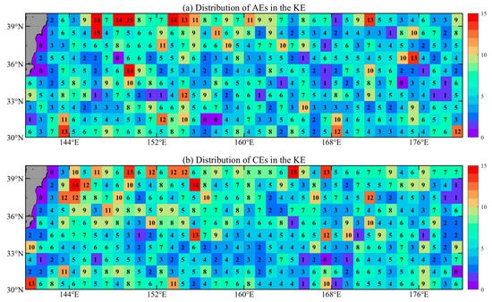
Figure 2.
The distribution of eddies first observed in the KE between 1 March 1993 and 29 February 2020. (a) is for AEs, while (b) is for CEs.
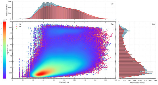
Figure 3.
(a) A statistical diagram of the eddy radius. (b) The probability density distribution for the radius and the amplitude of the mesoscale eddies in the KE region. (c) A statistical diagram of eddy amplitude. Red is for AEs, while blue is for CEs. The temporal coverage spans from 1 March 1993 to 29 February 2020.
3.2. Impact of Mesoscale Eddies on Sound Surface and Subsurface Channels
3.2.1. Sound Speed Anomaly Spatial Structure
Figure 4 presents the seasonal variations in sound speed anomaly structures of composite AEs and CEs with climatological amplitudes. In the study, we defined the seasons as follows: March to May as spring, June to August as summer, September to November as autumn, and December to February of the following year as winter. Results reveal that AEs exhibit a positive anomaly center at 365 m depth (+8.0 m/s), while CEs display a deeper (382 m) and stronger negative anomaly (−10.0 m/s), highlighting their enhanced vertical perturbation capacity. Seasonal analysis demonstrates systematic differences: For AEs, anomaly depths and magnitudes range from 360 m (+8.6 m/s) in summer to 401 m (+9.0 m/s) in autumn, with spring (364 m, +7.1 m/s) and winter (364 m, +7.3 m/s) showing intermediate values. In contrast, CEs exhibit maximum negative anomalies in summer (−11.0 m/s at 373 m) and autumn (−10.1 m/s at 383 m), with shallower perturbations in spring (406 m, −9.2 m/s) and winter (380 m, −9.5 m/s). Both eddy types induce distinct vertical displacements of isosonic lines—AEs depress and CEs elevate these contours, with perturbation intensity decaying radially from eddy centers. Annual mean sound speed extremes reach 1505 m/s (AEs) and 1490 m/s (CEs) at their respective cores. Notably, summer AEs uniquely generate surface-layer negative anomalies (−7.7 m/s at 71 m), while summer and autumn CEs simultaneously exhibit intense central perturbations and significant subsurface anomalies (−7.7 m/s at 71 m in summer; −8.5 m/s at 95 m in autumn), suggesting seasonally modulated vertical coupling mechanisms in eddy-induced acoustic environments. The results of sound speed anomaly distribution of composite eddies with amplitudes of 0.1–0.4 m in the KE region are illustrated in supporting information Figures S1–S4.
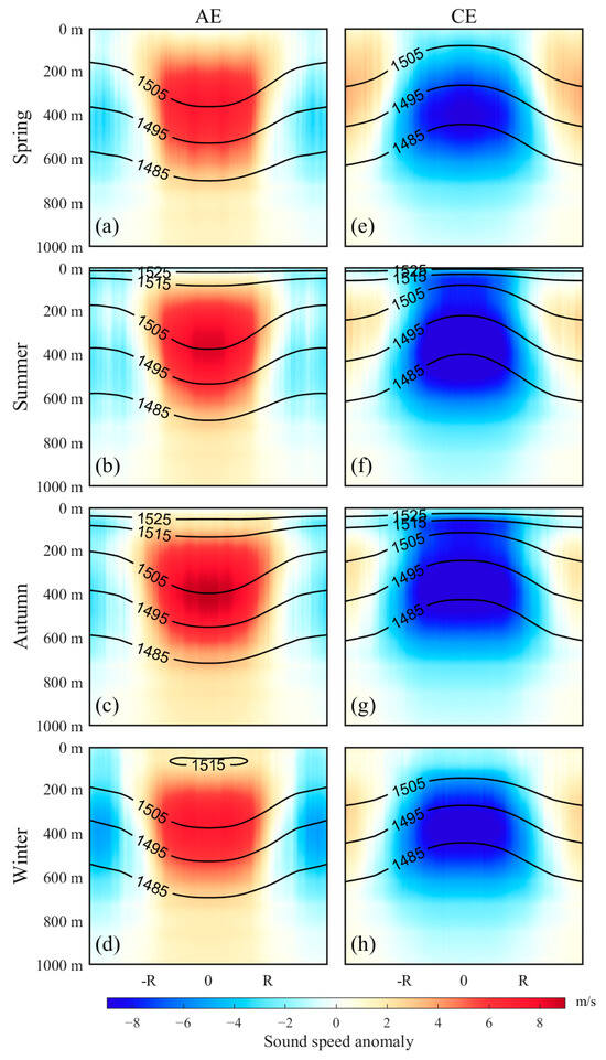
Figure 4.
The distribution of the sound speed anomalies for eddy composites of AEs and CEs in the KE region. The figure presents the average sound speed anomalies caused by eddies and the underwater sound field under the impact of eddies in different seasons, with (a–d) for AEs and (e–h) for CEs. The shadows show the sound speed anomalies of the eddies, while the solid black lines represent the underwater sound speed contours of the eddies. The units are as follows: m for depth; m/s for sound speed.
3.2.2. Seasonal Sound Channels
The sound speed profiles determine the presence of sound channels. The SC is defined as the water layer with a positive gradient distribution of sound speed under the surface, and its boundary is the depth of sound speed maximum. The width of the SSC is the distance between the channel top (bottom) (sound speed maximum) and the conjugate depth for that sound speed [26]. The amplitude of the eddy reflects the strength of the eddy; that is, the greater the amplitude of the eddy, the more significant its impact on the sound field. In this research, the eddy’s amplitudes from 0.1 m to 0.4 m are all calculated and the differences are mainly reflected in the depth and intensity of the sound channel (Figure 5). When the eddy’s amplitude reaches 0.4 m, the resulting change in the sound speed profile is sufficient to form a new sound channel through thermocline deformation (Figure 6 and Table 1).
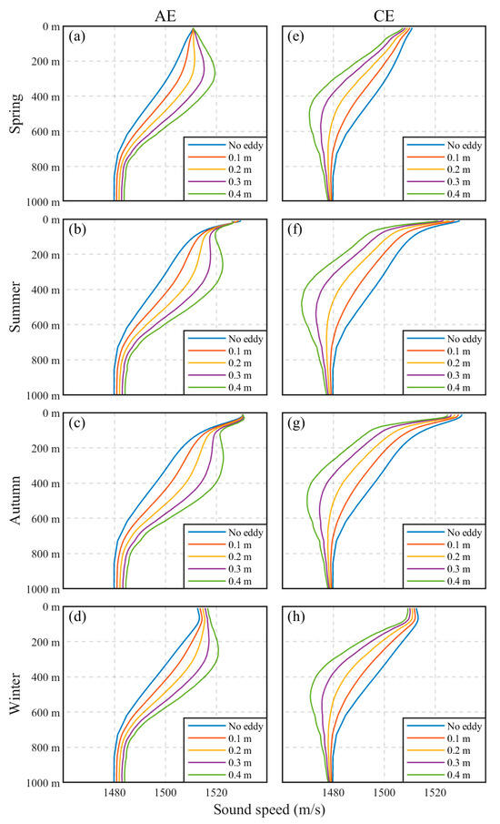
Figure 5.
Seasonal sound speed profiles in the center of eddies with various amplitudes. (a–d) The left column shows AEs, while (e–h) the right column shows CEs. The units are as follows: m for depth; m/s for sound speed.
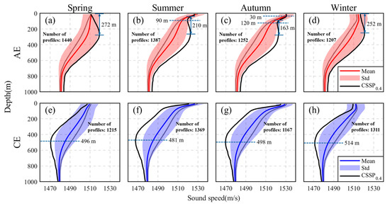
Figure 6.
Sound speed profiles in different seasons. (a–d) The top row shows AEs, while (e–h) the bottom row shows CEs. The solid red (blue) lines represent the mean sound speed profiles within a radius of eddies, while the shadows show standard deviation. The gray solid lines represent the sound speed profile of climate state, and the solid black lines represent the central sound speed profiles of eddies with the amplitude of 0.4 m. The units are as follows: m for depth; m/s for sound speed.

Table 1.
The distribution of the SCs/SSCs in the center of the eddies with the amplitude of 0.4 m and background field (no eddy). SSC is the depth of the channel axis of the subsurface sound channel, and SC is the width of the surface sound channel (also the magnitude of sonic layer depth (SLD)). A slash indicates that no SC or SSC exists.
For AEs with the amplitude of 0.4 m, due to the positive disturbance of the sound speed at the center, they can induce a thicker SC in spring and winter, an SSC in summer, and a special DC in autumn. When an AE with the amplitude of 0.4 m exists, the magnitude and the depth of the local maximum of sound speed are 1519.5 m/s and 272 m in spring, and 1520.9 m/s and 252 m in winter. Above the depth where the local maximum sound speed is located, there is a positive gradient distribution of sound speed, where an SC with a width equal to the depth of the maximum sound speed forms. In summer, a maximum sound speed of 1526.7 m/s appears at the sea surface, while a local maximum sound speed of 1522.6 m/s near the eddy center appears at 255 m deep, resulting in a minimum sound speed of 1519.6 m/s at a depth of 92 m between the two. Therefore, an SSC is generated with this depth as the axis, with a channel width of 210 m, confined between 43 and 253 m underwater. In autumn, a 30 m wide SC is formed, with the bottom of the sound channel located at the depth where the maximum sound speed of 1526.7 m/s is located. Similarly to summer, an SSC with the channel axis at a depth of 120 m is formed in autumn, confined between 94 and 257 m underwater, and the minimum sound speed is 1521.5 m/s.
CEs primarily exert their influence by diminishing the sound speed at their core, which consequently generates a local minimum in sound speed. This phenomenon leads to the elevation of the SOFAR. Under these conditions, the SOFAR transforms into an SSC, allowing sound waves to propagate over long distances within a shallower layer of seawater. When a CE with the amplitude of 0.4 m exists, the depth of the SSC axis and the local minimum sound speed are 496 m and 1470.7 m/s in spring, 481 m and 1467.6 m/s in summer, 498 m and 1469.8 m/s in autumn, and 514 m and 1471.0 m/s in winter. The original SC in winter is especially disintegrated due to the impact of CEs.
3.3. Characteristics of Sound Propagation in Sound Channels
3.3.1. Propagation Characteristics of Sound Waves in Eddy-Caused Sound Channels
The disturbances caused by eddies diminish as the distance from the eddy center increases, thus their impact on sound propagation is primarily concentrated at the eddy center. To analyze the sound propagation characteristics at various positions of eddies (with the amplitude of 0.4 m), Figure 7 illustrates the sound propagation loss as sound waves radiate outward from the eddy center. The radius of the eddies is assumed to be 100 km, the sound source frequency is 3000 Hz, and the sound sources are set at the sea surface (10 m deep) or on the axis of the SSCs.
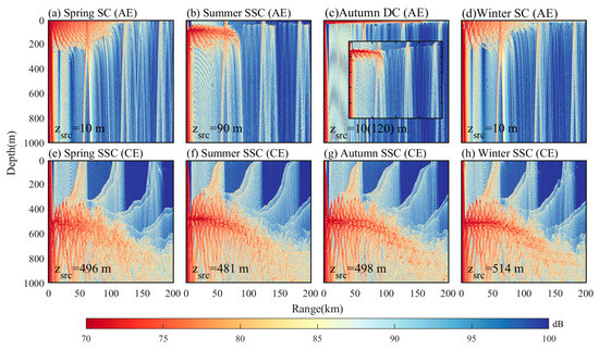
Figure 7.
Transmission loss in the SCs (SSCs) generated by eddies with the amplitude of 0.4 m in different seasons. (a–d) The top row shows AEs, while (e–h) the bottom row shows CEs. In subfigure (c), the subpanel represents the autumn SSC, while the main panel represents the SC. The units are as follows: m for depth; km for range; and dB for transmission loss.
The results indicate that for AEs, SCs formed in spring and winter extend 100 km outward from the eddy center (i.e., one time the normalized radius). Meanwhile, due to the greater sound speed gradient within the spring SC compared to winter, it has a stronger binding effect on sound energy, with sound rays reflecting more frequently within the sound channel. For the SSCs formed in summer and autumn, the channel in summer extends 80 km outward from the eddy center, while in autumn it is 75 km. Meanwhile, the findings demonstrate that the SC induced by AEs in autumn extends 170 km outward from the eddy center, with an average sound propagation loss of 70~75 dB within the channel. The average sound transmission loss within the sound channels generated by AEs in four seasons is 75~80 dB.
Regarding the SSC generated by CEs, it exhibits a bending feature that the sound channel is gradually pressed down from the eddy center to the outside, which can be interpreted as the weakening of the eddy’s lifting effect on the SOFAR axis as the distance from the eddy center increases, with the SSC gradually transitioning to the deep sound channel. It is noteworthy that, in comparison to the other three seasons, the sound channel formed in spring exhibits a weaker capacity to confine sound energy, with greater transmission loss and more significant divergence of sound rays. This phenomenon can be attributed to the smaller negative sound speed gradient in the layer immediately above the SSC axis during the spring season. The results demonstrate that the sound energy in spring is predominantly concentrated within the 0~50 km range, while in other seasons, the concentration extends up to 100 km. The average transmission loss of the sound energy in the sound channel generated by the CEs in four seasons is 75~80 dB. The sound transmission loss induced by eddies with amplitudes of 0.1–0.3 m was computed, with the corresponding results provided in the supporting materials (supporting information Figures S11–S14).
3.3.2. DC Phenomenon in Autumn
A distinctive DC phenomenon emerges in autumn, characterized by the simultaneous presence of both an SC and an SSC. This configuration arises from the interplay between the ambient sound speed field and AE perturbations. The autumn sound speed profile features a high-speed surface layer with a thickened isosonic zone. AE-induced disturbances generate an additional sound speed maximum at the eddy core, while creating a localized minimum between this subsurface peak and the upper-ocean high-velocity layer, thereby establishing the SSC. Concurrently, within the upper isosonic layer, stronger sound speed perturbations in the lower stratum compared to the upper section facilitate a surface-positive sound speed gradient when eddy intensity exceeds critical thresholds. This vertical contrast enables SC formation through surface sound speed maximization. The synergistic effects of these processes ultimately produce twin sound channels beneath the eddy structure, as illustrated in Figure 8.
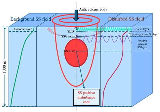
Figure 8.
A diagram of the formation of the DC in autumn. SS is the abbreviation for sound speed.
4. Discussion
4.1. Regional Variability of Eddy-Induced Acoustic Effects
The unique acoustic phenomena generated by mesoscale eddies are caused by the specific sound speed disturbance structures inherent to eddies, and the thermohaline structure of eddies is closely related to the thermohaline background field of the sea area [27,28]. Therefore, mesoscale eddies in different sea areas could produce different acoustic effects. Taking the KE as example, the thermohaline background field is characterized by a permanent thermocline at 400 m depth, with seasonal thermoclines at 30 m in summer and 50 m in winter. The horizontal thermohaline gradients also exhibit a maximum at 300 m depth (Figure 9). The special thermohaline distribution uniquely affects the generation and extinction of SCs and SSCs. Moreover, it can be inferred that the acoustic effects induced by mesoscale eddies are region-dependent. Here, two particularly special sea areas are selected for discussion: the Subtropical Countercurrent (STCC) and the Gulf Stream (GS). According to the research findings of Chen et al. [9], for the eddies in the STCC, they have a dual-core disturbance structure at 100 m and 400 m, which allows one to speculate that when the eddy’s disturbance is sufficient, AEs will promote the formation of an SC at 100 m, while forming an SSC between 100 m and 400 m; CEs, on the other hand, are conducive to the formation of an SSC at 100 m and lift the SOFAR axis to a greater depth. For the eddies in the GS, the disturbance core is 700 m deep, and such a deeper core has a weaker impact on SCs. However, for AEs, the local maximum of sound speed produced by the disturbance core and the high sound speed layer at the sea surface may result in a local minimum of sound speed between them, thus forming an SSC above 700 m. The generalizability of the findings to other sea areas with active eddies warrants further investigation, contingent upon the availability of equivalent altimetry-derived eddy datasets and complementary underwater hydrographic observations. Methodological frameworks developed herein could be cautiously extended to these regions, though regional discrepancies in mesoscale dynamics and stratification patterns may necessitate adaptive parameterization.
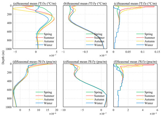
Figure 9.
The seasonal mean thermohaline gradient in the KE region. From left to right, the latitudinal, longitudinal, and vertical gradients are represented. (a–c) The top row shows the temperature, while (d–f) the bottom row shows the salinity. The units are as follows: m for depth; °C/m for temperature gradient; psu/m for salinity gradient.
4.2. Verification of Composite Results with Actual Profiles
Due to limitations in underwater observational data, the number of Argo profiles that can be matched with eddies of varying amplitudes is inconsistent, which makes it challenging to directly composite eddies of corresponding amplitudes by using Argo profiles that match the amplitudes of the eddies. Therefore, the methodology implemented in this study comprises two sequential phases: (1) compositing a dimensionless, amplitude-normalized composite eddy structure by statistically integrating all available Argo profiles within the eddy-centric coordinate system, followed by (2) amplitude restoration through scaling transformations to reconstruct eddies with site-specific amplitudes while preserving the intrinsic thermohaline perturbation patterns.
To assess the reliability of the result from composite eddies, a statistical analysis was conducted on Argo profiles that are located within one radius of eddies of varying amplitudes. Our analysis stratified Argo profiles into four distinct amplitude ranges (0.05–0.15 m, 0.15–0.25 m, 0.25–0.35 m, and 0.35–0.45 m) corresponding to composite eddies with normalized amplitudes (0.1–0.4 m), respectively. Figure 10 shows examples of sound speed profiles (corresponding to eddies with amplitudes ranging from 0.35 to 0.45 m) calculated from Argo data. Since the selected profiles are confined within a normalized radius, their captured eddy perturbation intensities do not uniformly represent the central values of the eddies. Consequently, their averaged values exhibit certain deviations from idealized results, but still demonstrate trends consistent with previous findings. Notably, for some individual profiles, the results align with prior observations in significant measure. We thus conclude that the composite results are reasonably reliable within the methodological constraints. Additional validation results are available in the supporting information Figures S5–S10.
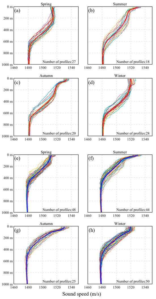
Figure 10.
The collection of sound speed profiles within a normalized radius of AEs and CEs with amplitudes from 0.35 m to 0.45 m. Red (blue) lines are the average for AEs (CEs). (a–d) show profiles of AEs, while (e–h) show profiles of CEs. The units are as follows: m for depth; m/s for sound speed.
5. Conclusions
This study has achieved a comprehensive quantitative analysis of eddy impacts on sound channels in the KE, establishing specific acoustic parameters for eddy-induced channels and revealing distinct seasonal variations in upper-ocean channel distributions. The research not only advances understanding of upper-ocean acoustic–eddy interactions by partially overcoming data scarcity constraints through innovative composite analysis methods, but also provides robust theoretical foundations for critical applications including sonar optimization and underwater detection system design.
The results show that the influence of eddies on the upper-ocean sound channel is non-negligible. They affect the generation and decay of the sound channels by altering the distribution pattern of the sound speed in seawater. Conducting composite analysis of eddies in the KE by using different datasets, the sound speed anomalies of eddies with different polarities in the region during different seasons are obtained. It was found that the average disturbance center of AEs is 365 m deep with a magnitude of 8.0 m/s, while those of the CEs are 382 m and −10.0 m/s. Taking eddies with the amplitude of 0.4 m as an example, the CE lifts the SOFAR axis to approximately 500 m, thereby forming an SSC, while in winter it disrupts the SC; the AE forms an SC with a width of 272 m in spring and 252 m in winter. In summer, it forms an SSC with a sound channel axis at a depth of 92 m and a width of 210 m. In autumn, it forms a unique DC, where both the SC and SSC exist simultaneously, with the SC width being 30 m, the SSC width being 163 m, and the sound channel axis at a depth of 120 m. On the other hand, due to the non-uniform distribution of eddy disturbances in the horizontal direction, the sound channels they cause will gradually weaken as the distance from the center increases. For SCs formed by AEs, they extend 100 km outward from the eddy center in spring and winter, and 170 km in autumn. SSCs formed by CEs will be depressed at a distance of 100 km from the eddy center, gradually returning to the SOFAR. Therefore, the research findings can offer practical implications for underwater operations. Satellite-derived surface observation data of eddies can be utilized to infer their underwater structures. This allows for adjustments in sonar parameters or positioning guided by our work. Even though such predictions may involve some degree of error, they still provide actionable guidance. For example, sonar systems could leverage AEs to extend surface detection ranges in spring/winter through enhanced SCs.
Additionally, the study discusses the potential impacts of mesoscale eddies in other sea areas on SCs and SSCs. Focusing on the STCC and the GS, which are regions with active eddy activity, the study analyses the sound speed structure of the eddies in these regions to infer the possible effects on sound channels in the upper ocean. This further expands the scope of the research findings presented in the paper.
On the other hand, while the eddy synthesis in this study assumes central symmetry of eddies, actual observations reveal that the upper-layer temperature anomaly structure exhibits meridional differences due to significant zonal variations in upper-ocean temperatures [28]. These anomalies frequently manifest as dipole structures, resulting in more nuanced variations in upper-ocean acoustic effects. This study primarily focuses on investigating the seasonal variations of upper-ocean sound channel structures associated with vortices, and therefore simplifies this particular aspect. And in the conclusion verification, quantitative verification was restricted to historical Argo data, lacking synchronized in situ acoustic transmission measurements to directly corroborate predicted SC/SSC formations. Subsequent research should continue to refine and deepen these investigations to derive more novel conclusions.
Supplementary Materials
The following supporting information can be downloaded at: https://www.mdpi.com/article/10.3390/rs17081360/s1, Figure S1: Sound speed anomaly distribution of composite eddies with amplitudes of 0.1 m in the KE region; Figure S2: Sound speed anomaly distribution of composite eddies with amplitudes of 0.2 m in the KE region; Figure S3: Sound speed anomaly distribution of composite eddies with amplitudes of 0.3 m in the KE region; Figure S4: Sound speed anomaly distribution of composite eddies with amplitudes of 0.4 m in the KE region; Figure S5: Collection of sound speed profiles within a normalized radius of AEs with the amplitudes from 0.05 m to 0.15 m; Figure S6: Collection of sound speed profiles within a normalized radius of AEs with the amplitudes from 0.15 m to 0.25 m; Figure S7: Collection of sound speed profiles within a normalized radius of AEs with the amplitudes from 0.25 m to 0.35 m; Figure S8: Collection of sound speed profiles within a normalized radius of CEs with the amplitudes from 0.05 m to 0.15 m; Figure S9: Collection of sound speed profiles within a normalized radius of CEs with the amplitudes from 0.15 m to 0.25 m; Figure S10: Collection of sound speed profiles within a normalized radius of CEs with the amplitudes from 0.25 m to 0.35 m; Figure S11: Transmission loss with no eddy in different seasons; Figure S12: Transmission loss under impact of eddies with the amplitude of 0.1 m in different seasons; Figure S13: Transmission loss under impact of eddies with the amplitude of 0.2 m in different seasons; Figure S14: Transmission loss under impact of eddies with the amplitude of 0.3 m in different seasons.
Author Contributions
Programs, Y.W. (Youwei Wu) and W.C.; data curation, Y.W. (Youwei Wu) and W.C.; writing—original draft preparation, Y.W. (Youwei Wu); writing—review and editing, Y.Z., M.H., Y.W. (Yang Wang), W.G., Z.L. and Y.S.; directing: Y.Z. and W.C. All authors have read and agreed to the published version of the manuscript.
Funding
This research received no external funding.
Data Availability Statement
The authors confirm that the data supporting the findings of this study are available within the article and its Supplementary Materials. The Mesoscale Eddy Trajectories Atlas product that supports this study can be accessed at https://doi.org/10.24400/527896/a01-2022.006.220209 (accessed on 1 December 2024) [29]. The Argo dataset that supports this study can be accessed at https://doi.org/10.17882/42182 (accessed on 1 December 2024) [30]. The SODA3.4.2 data that support this study can be accessed at https://www2.atmos.umd.edu/~ocean/index_files/soda3.4.2.0_mn_download.htm (accessed on 1 December 2024) [31].
Acknowledgments
The authors would like to acknowledge the Archiving, Validation and Interpretation of Satellite Oceanographic (AVISO) for providing the mesoscale eddy trajectory atlas used in this work, as well as the Array for Real-time Geostrophic Oceanography (Argo) and the Simple Ocean Data Assimilation (SODA) for providing the oceanographic data. In addition, the authors would like to thank the Ocean Acoustics Library for providing the BELLHOP acoustic toolbox, which is available for download at http://oalib.hlsresearch.com/AcousticsToolbox/ (accessed on 1 December 2024) [32].
Conflicts of Interest
The authors declare no conflicts of interest.
Abbreviations
The following abbreviations are used in this manuscript:
| AE | Anticyclonic eddy |
| CE | Cyclonic eddy |
| DC | Dual-duct sound channel |
| KE | Kuroshio Extension |
| SC | Surface sound channel |
| SLD | Sonic layer depth |
| SS | Sound speed |
| SSC | Subsurface sound channel |
References
- Chelton, D.B.; Schlax, M.G.; Samelson, R.M. Global Observations of Nonlinear Mesoscale Eddies. Prog. Oceanogr. 2011, 91, 167–216. [Google Scholar] [CrossRef]
- Chelton, D.B.; Schlax, M.G.; Samelson, R.M.; de Szoeke, R.A. Global Observations of Large Oceanic Eddies. Geophys. Res. Lett. 2007, 34. [Google Scholar] [CrossRef]
- Manche, S.S.; Nayak, R.K.; Sikhakolli, R.; Bothale, R.V.; Chauhan, P. Characteristics of Mesoscale Eddies and Their Evolution in the North Indian Ocean. Prog. Oceanogr. 2024, 221, 103213. [Google Scholar] [CrossRef]
- Wang, G.; Su, J.; Chu, P.C. Mesoscale eddies in the South China Sea observed with Altimeter Data. Geophys. Res. Lett. 2003, 30. [Google Scholar] [CrossRef]
- Li, J.; Wang, G.; Xue, H.; Wang, H. A simple predictive model for the eddy propagation trajectory in the northern South China Sea. Ocean Sci. 2019, 15, 401–412. [Google Scholar] [CrossRef]
- Dai, J.; Wang, H.; Zhang, W.; An, Y.; Zhang, R. Observed Spatiotemporal Variation of Three-Dimensional Structure and Heat/Salt Transport of Anticyclonic Mesoscale Eddy in Northwest Pacific. J. Oceanol. Limnol. 2020, 38, 1654–1675. [Google Scholar] [CrossRef]
- Sun, W.; Dong, C.; Wang, R.; Liu, Y.; Yu, K. Vertical Structure Anomalies of Oceanic Eddies in the Kuroshio Extension Region. J. Geophys. Res. Ocean 2017, 122, 1476–1496. [Google Scholar] [CrossRef]
- Chaigneau, A.; Le Texier, M.; Eldin, G.; Grados, C.; Pizarro, O. Vertical Structure of Mesoscale Eddies in the Eastern South Pacific Ocean: A Composite Analysis from Altimetry and Argo Profiling Floats(Article). J. Geophys. Res. Ocean 2011, 116, C11025–C11040. [Google Scholar] [CrossRef]
- Chen, W.; Zhang, Y.; Liu, Y.; Ma, L.; Wang, H.; Ren, K.; Chen, S. Parametric Model for Eddies-Induced Sound Speed Anomaly in Five Active Mesoscale Eddy Regions. J. Geophys. Res. Ocean 2022, 127. [Google Scholar] [CrossRef]
- Khan, S.; Song, Y.; Huang, J.; Piao, S. Analysis of Underwater Acoustic Propagation under the Influence of Mesoscale Ocean Vortices. J. Mar. Sci. Eng. 2021, 9, 799. [Google Scholar] [CrossRef]
- DeFerrari, H.; Olson, D. The Influence of Mesoscale Eddies on Shallow Water Acoustic Propagation. J. Acoust. Soc. Am. 2003, 114, 2376. [Google Scholar] [CrossRef]
- Vastano, A.C.; Owens, G.E. On the Acoustic Characteristics of a Gulf Stream Cyclonic Ring. J. Phys. Oceanogr. 1973, 3, 470–478. [Google Scholar] [CrossRef]
- Weinberg, N.L.; Zabalgogeazcoa, X. Coherent Ray Propagation through a Gulf Stream Ring. J. Acoust. Soc. Am. 1977, 62, 888–894. [Google Scholar] [CrossRef]
- Henrick, R.F.; Jacobson, M.J.; Siegmann, W.L. General Effects of Currents and Sound-Speed Variations on Short-Range Acoustic Transmission in Cyclonic Eddies. J. Acoust. Soc. Am. 1980, 67, 121–134. [Google Scholar] [CrossRef]
- Zhang, X.; Cheng, C.; Qiu, R. Abnormal Features of the Convergence Zone Caused by the Cold Eddy in Western Pacific. Mar. Sci. Bull. 2015, 34, 130–137. [Google Scholar] [CrossRef]
- Chen, W.; Zhang, Y.; Liu, Y.; Wu, Y.; Zhang, Y.; Ren, K. Observation of a Mesoscale Warm Eddy Impacts Acoustic Propagation in the Slope of the South China Sea. Front. Mar. Sci. 2022, 9. [Google Scholar] [CrossRef]
- Li, Q.; Han, X.; Cao, R.; Wei, Z. An Analysis of Acoustic Propagation Characteristics of Dual-Duct Waveguide in the Arctic. J. Harbin Eng. Univ. 2024, 45, 1280–1287. [Google Scholar] [CrossRef]
- Mercer, J.A.; Booker, J.R. Long-Range Propagation of Sound through Oceanic Mesoscale Structures. J. Geophys. Res. Ocean 1983, 88, 689–699. [Google Scholar] [CrossRef]
- Xu, A.; Dong, C.; Yu, F.; Zhang, Y.; Nan, F.; Ren, Q.; Chen, Z. Effects of a Subsurface Eddy on Acoustic Propagation in the Northwestern Pacific Ocean. J. Mar. Sci. Eng. 2023, 11, 1785. [Google Scholar] [CrossRef]
- Colosi, J.A.; Rudnick, D.L. Observations of Upper Ocean Sound-Speed Structures in the North Pacific and Their Effects on Long-Range Acoustic Propagation at Low and Mid-Frequencies. J. Acoust. Soc. Am. 2020, 148, 2040. [Google Scholar] [CrossRef]
- Liu, J.; Piao, S.; Gong, L.; Zhang, M.; Guo, Y.; Zhang, S. The Effect of Mesoscale Eddy on the Characteristic of Sound Propagation. J. Mar. Sci. Eng. 2021, 9, 787. [Google Scholar] [CrossRef]
- Li, J.; Zhang, R.; Chen, Y.; Jin, B. Ocean Mesoscale Eddy Modeling and Its Application in Studying the Effect on Underwater Acoustic Propagation. Mar. Sci. Bull. 2011, 30, 37–46. [Google Scholar] [CrossRef]
- Dong, D.; Brandt, P.; Chang, P.; Schutte, F.; Yang, X.; Yan, J.; Zeng, J. Mesoscale Eddies in the Northwestern Pacific Ocean: Three-Dimensional Eddy Structures and Heat/Salt Transports. J. Geophys. Res. Ocean 2017, 122, 9795–9813. [Google Scholar] [CrossRef]
- Keppler, L.; Cravatte, S.; Chaigneau, A.; Pegliasco, C.; Gourdeau, L.; Singh, A. Observed Characteristics and Vertical Structure of Mesoscale Eddies in the Southwest Tropical Pacific. J. Geophys. Res. Ocean 2018, 123, 2731–2756. [Google Scholar] [CrossRef]
- Yang, G.; Wang, F.; Li, Y.; Lin, P. Mesoscale Eddies in the Northwestern Subtropical Pacific Ocean: Statistical Characteristics and Three-Dimensional Structures. J. Geophys. Res. Ocean 2013, 118, 1906–1925. [Google Scholar] [CrossRef]
- Duda, T.F.; Zhang, W.G.; Lin, Y.-T. Effects of Pacific Summer Water Layer Variations and Ice Cover on Beaufort Sea Underwater Sound Ducting. J. Acoust. Soc. Am. 2021, 149, 2117. [Google Scholar] [CrossRef]
- Lin, X.; Qiu, Y.; Ni, X.; Lin, W.; Cherry, A. Three-Dimensional Climatological Structures of the Arabian Sea Eddies and Eddy-Induced Flux. J. Ocean. Univ. China 2023, 22, 874–885. [Google Scholar] [CrossRef]
- Zu, Y.; Sun, S.; Zhao, W.; Li, P.; Liu, B.; Fang, Y.; Samah, A.A. Seasonal Characteristics and Formation Mechanism of the Thermohaline Structure of Mesoscale Eddy in the South China Sea. Acta Oceanol. Sin. 2019, 38, 29–38. [Google Scholar] [CrossRef]
- Pegliasco, C.; Delepoulle, A.; Mason, E.; Morrow, R.; Faugere, Y.; Dibarboure, G. META3.1exp: A New Global Mesoscale Eddy Trajectory Atlas Derived from Altimetry. Earth Syst. Sci. Data 2022, 14, 1087–1107. [Google Scholar] [CrossRef]
- Wong, A.P.S.; Wijffels, S.E.; Riser, S.C.; Pouliquen, S.; Hosoda, S.; Roemmich, D.; Gilson, J.; Johnson, G.C.; Martini, K.; Murphy, D.J.; et al. Argo Data 1999–2019: Two Million Temperature-Salinity Profiles and Subsurface Velocity Observations From a Global Array of Profiling Floats. Front. Mar. Sci. 2020, 7. [Google Scholar] [CrossRef]
- Carton, J.A.; Chepurin, G.A.; Chen, L. SODA3: A New Ocean Climate Reanalysis. J. Clim. 2018, 31, 6967–6983. [Google Scholar] [CrossRef]
- Pisha, L.A.; Snider, J.; Jackson, K.; Jaffe, J.S. Introducing bellhopcxx/bellhopcuda: Modern, parallel BELLHOP(3D). J. Acoust. Soc. Am. 2023, 153, A218. [Google Scholar] [CrossRef]
Disclaimer/Publisher’s Note: The statements, opinions and data contained in all publications are solely those of the individual author(s) and contributor(s) and not of MDPI and/or the editor(s). MDPI and/or the editor(s) disclaim responsibility for any injury to people or property resulting from any ideas, methods, instructions or products referred to in the content. |
© 2025 by the authors. Licensee MDPI, Basel, Switzerland. This article is an open access article distributed under the terms and conditions of the Creative Commons Attribution (CC BY) license (https://creativecommons.org/licenses/by/4.0/).